
Analysing the Impact of Climate Change on Hydrological Ecosystem Services in Laguna del Sauce (Uruguay) Using the SWAT Model and Remote Sensing Data

 , , and
Abstract
:
1. Introduction
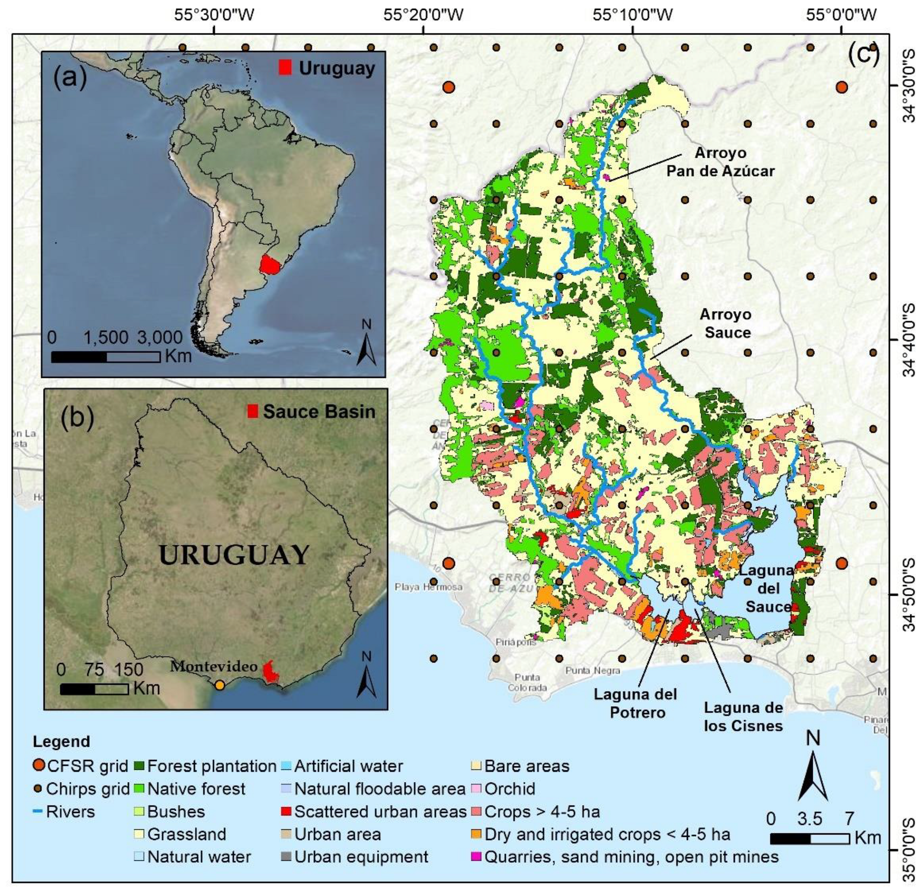
2. Study Area
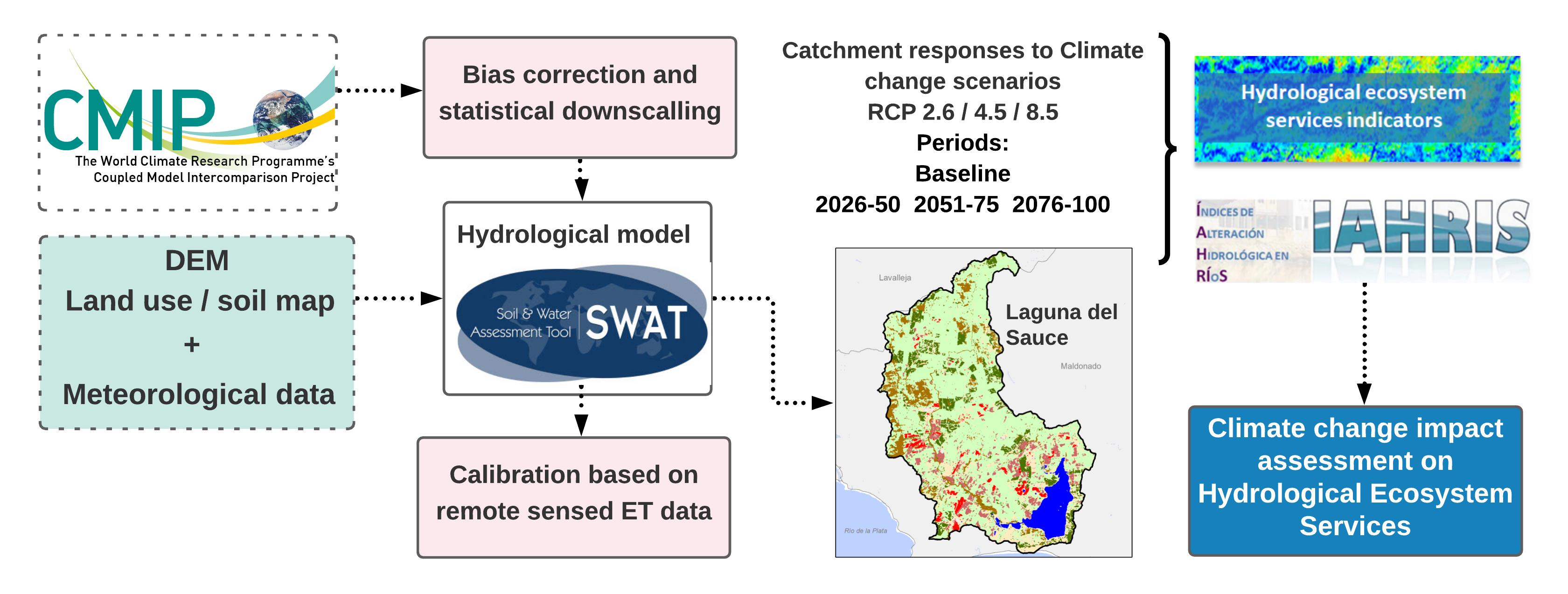
3. Materials and Methods
3.1. SWAT Model Implementation
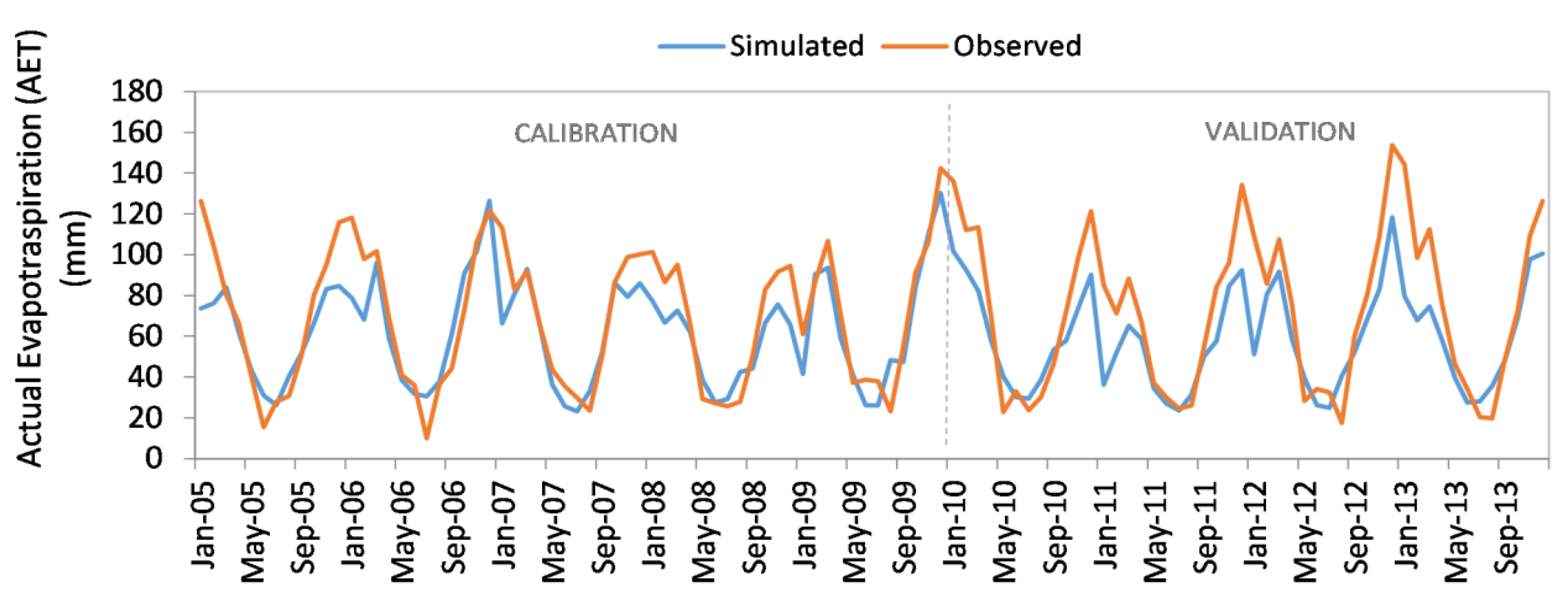
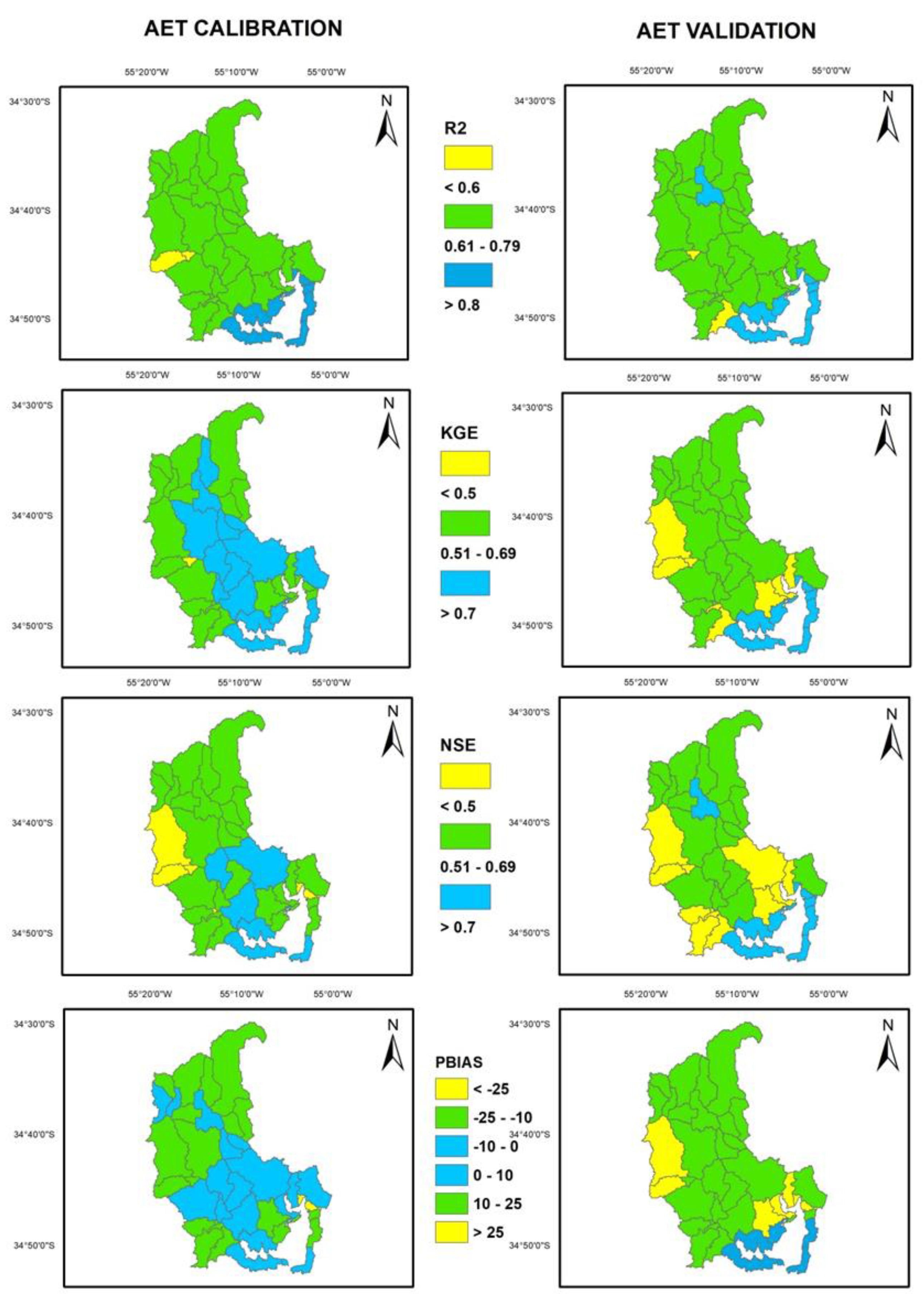
3.2. Model Setup, Calibration and Validation
3.3. Climate Change Projections
3.4. Indicators for Ecosystem Services Assessment
3.4.1. Estimation of Blue and Green Water Using SWAT Model
3.4.2. Description of Parameters from IAHRIS Used for Flood Analysis
4. Results and Discussion
4.1. Calibration and Validation
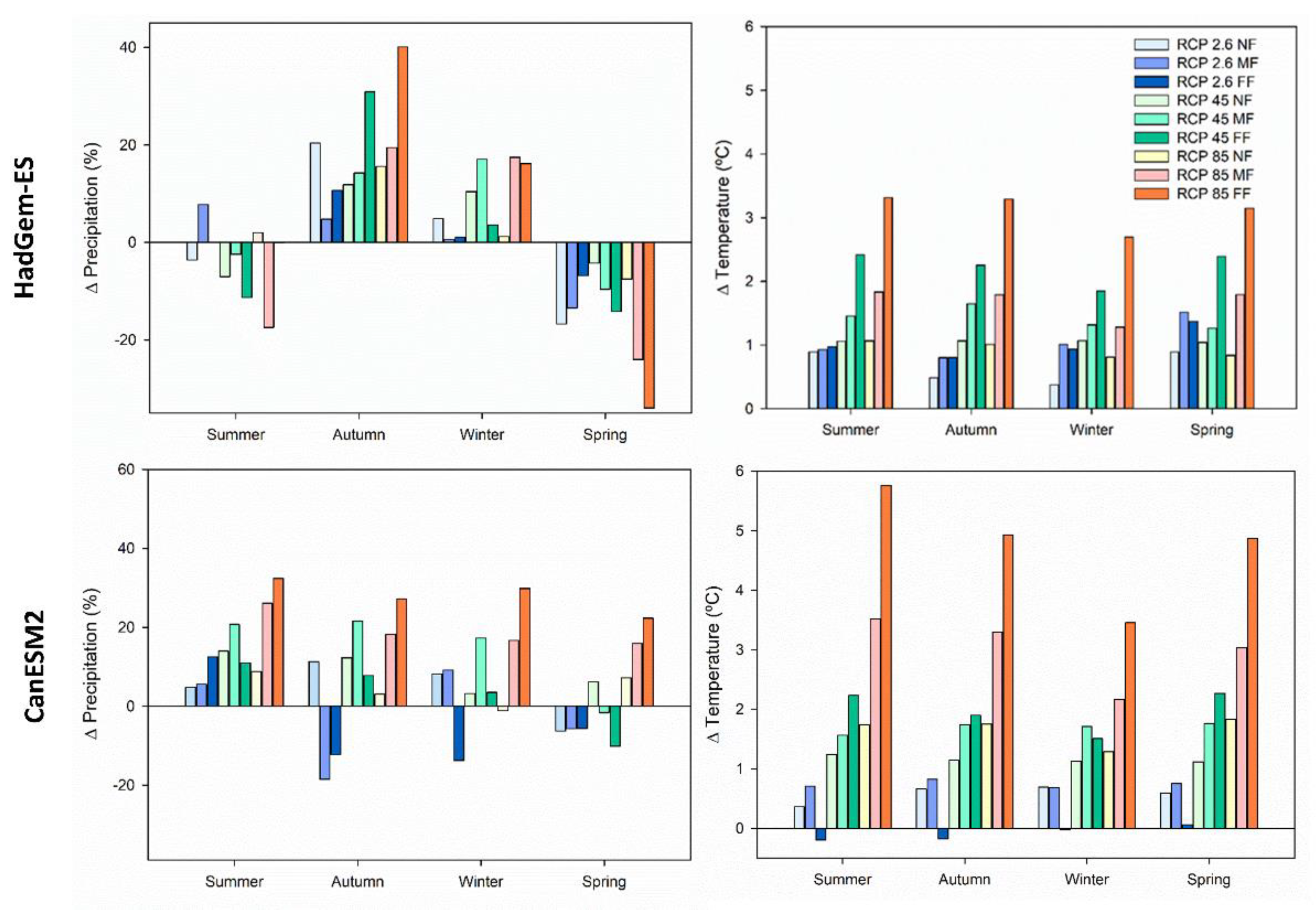
4.2. Climate Change Impacts on Rainfall and Temperature
4.3. Effects on Hydrological Ecosystem Services
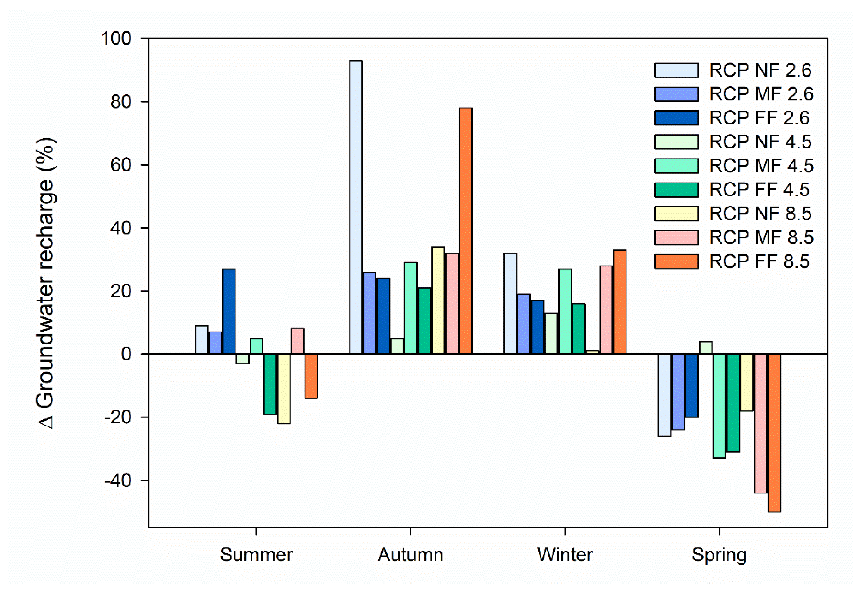
4.3.1. Water Regulation and Supply
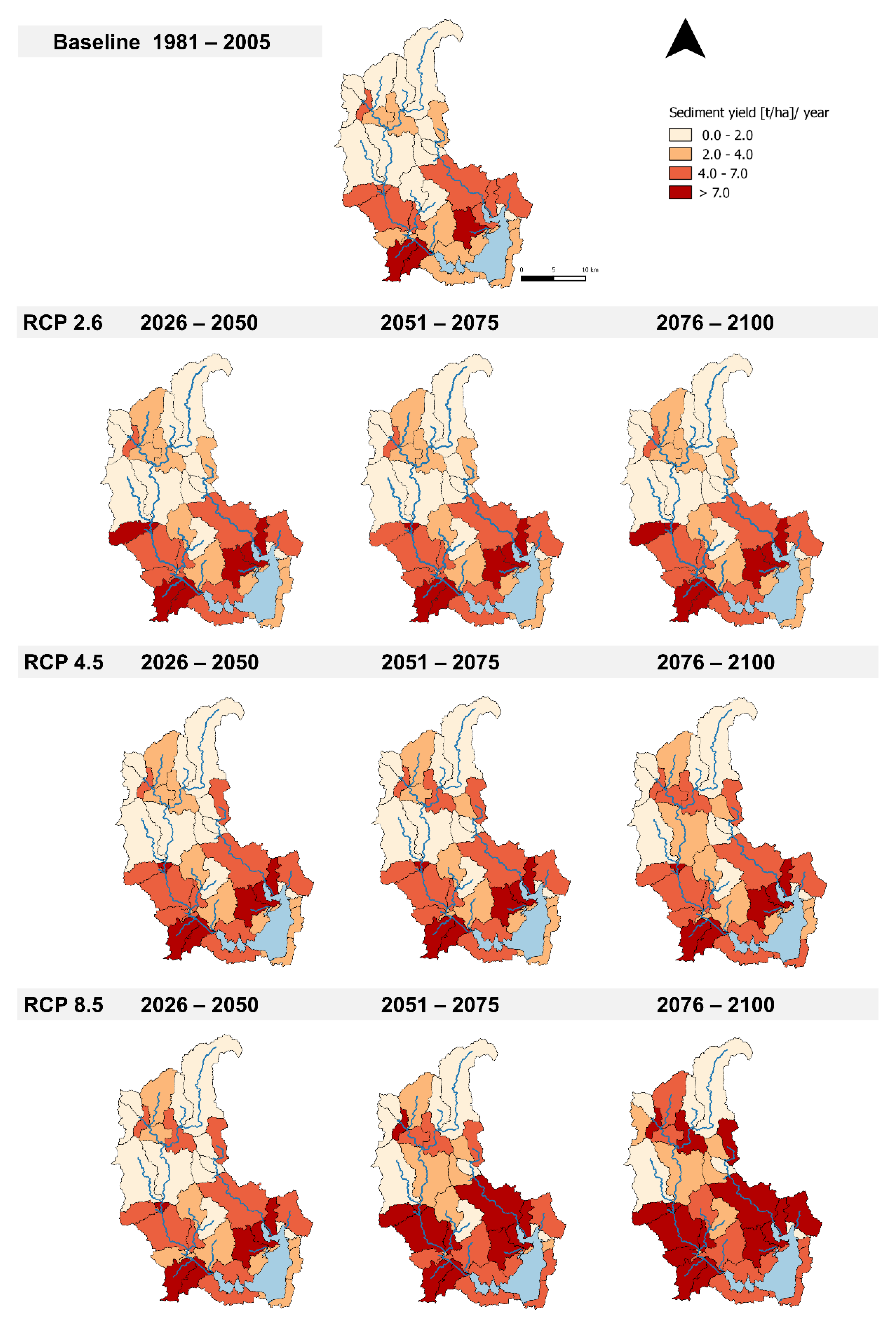
4.3.2. Soil Erosion Control
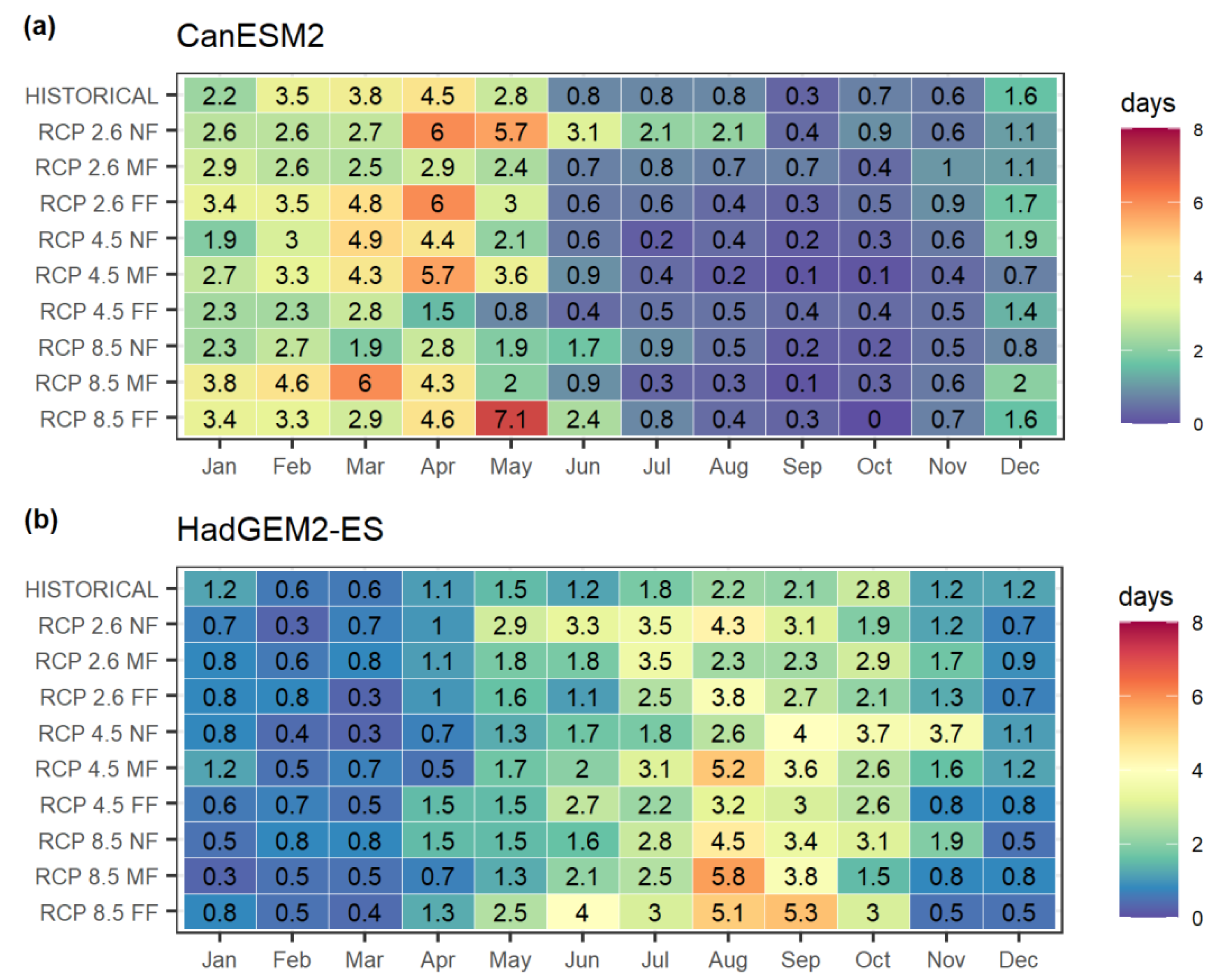
4.3.3. Natural Hazard Mitigation
4.4. Limitations of the Study and Future Improvements
5. Conclusions
Author Contributions
Funding
Institutional Review Board Statement
Informed Consent Statement
Data Availability Statement
Acknowledgments
Conflicts of Interest
References
- Liu, J.; Kattel, G.; Arp, H.P.H.; Yang, H. Towards threshold-based management of freshwater ecosystems in the context of climate change. Ecol. Model. 2015, 318, 265–274. [Google Scholar] [CrossRef] [Green Version]
- Díazo, S.; Settele, J.; Brondízio, E.; Ngo, H.T.; Guèze, M.; Agard, J.; Arneth, A.; Balvanera, P.; Brauman, K.; Butchart, S. Summary for Policymakers of the Global Assessment Report on Biodiversity and Ecosystem Services; Intergovernmental Science-Policy Platform on Biodiversity and Ecosystem Services (IPBES): Paris, France, 2019. [Google Scholar]
- Ávila-García, D.; Morató, J.; Pérez-Maussán, A.I.; Santillán-Carvantes, P.; Alvarado, J.; Comín, F.A. Impacts of alternative land-use policies on water ecosystem services in the Río Grande de Comitán-Lagos de Montebello watershed, Mexico. Ecosyst. Serv. 2020, 45, 101179. [Google Scholar] [CrossRef]
- MEA. Millennium ecosystem assessment. In Ecosystems and Human Well-Being: Synthesis; Island Press: Washington, DC, USA, 2005; ISBN 1-56973-597-2. [Google Scholar]
- Ostrom, E. A general framework for analyzing sustainability of social-ecological systems. Science 2009, 325, 419–422. [Google Scholar] [CrossRef] [PubMed]
- Brauman, K.A.; Daily, G.C.; Duarte, T.K.E.; Mooney, H.A. The nature and value of ecosystem services: An overview highlighting hydrologic services. Ann. Rev. Environ. Res. 2007, 32, 67–98. [Google Scholar] [CrossRef]
- Fan, M.; Shibata, H.; Wang, Q. Optimal conservation planning of multiple hydrological ecosystem services under land use and climate changes in Teshio river watershed, northernmost of Japan. Ecol. Indic. 2016, 62, 1–13. [Google Scholar] [CrossRef]
- Stocker, T.F.; Qin, D.; Plattner, G.K.; Tignor, M.M.; Allen, S.K.; Boschung, J.; Nauels, A.; Xia, Y.; Bex, V.; Midgley, P.M.; et al. Climate Change 2013: The Physical Science Basis. Contribution of Working Group I to the Fifth Assessment Report of IPCC the Intergovernmental Panel on Climate Change; Cambridge University Press: Cambridge, UK, 2014. [Google Scholar] [CrossRef] [Green Version]
- Senent-Aparicio, J.; Pérez-Sánchez, J.; Carrillo-García, J.; Soto, J. Using SWAT and Fuzzy TOPSIS to Assess the Impact of Climate Change in the Headwaters of the Segura River Basin (SE Spain). Water 2017, 9, 149. [Google Scholar] [CrossRef] [Green Version]
- Hack, J. Application of payments for hydrological ecosystem services to solve problems of fit and interplay in integrated water resources management. Water Inter. 2015, 40, 929–948. [Google Scholar] [CrossRef]
- Francesconi, W.; Srinivasan, R.; Pérez-Miñana, E.; Willcock, S.P.; Quintero, M. Using the Soil and Water Assessment Tool (SWAT) to model ecosystem services: A systematic review. J. Hydrol. 2016, 535, 625–636. [Google Scholar] [CrossRef]
- Hoyer, R.; Chang, H. Assessment of freshwater ecosystem services in the Tualatin and Yamhill basins under climate change and urbanization. Appl. Geogr. 2014, 53, 402–416. [Google Scholar] [CrossRef]
- Bennett, E.M.; Peterson, G.D.; Gordon, L.J. Understanding relationships among multiple ecosystem services. Ecol. Lett. 2009, 12, 1394–1404. [Google Scholar] [CrossRef] [PubMed]
- Peterson, G.D.; Cumming, G.S.; Carpenter, S.R. Scenario planning: A tool for conservation in an uncertain world. Cons. Biol. 2003, 17, 358–366. [Google Scholar] [CrossRef] [Green Version]
- Thompson, J.R.; Wiek, A.; Swanson, F.J.; Carpenter, S.R.; Fresco, N.; Hollingsworth, T.; Spies, T.A.; Foster, D.R. Scenario studies as a synthetic and integrative research activity for long-term ecological research. BioScience 2012, 62, 367–376. [Google Scholar] [CrossRef] [Green Version]
- Lüke, A.; Hack, J. Modelling Hydrological Ecosystem Services–A state of the art model comparison. Hydrol. Earth Syst. Sci. Dis. 2017, 1–29. [Google Scholar] [CrossRef]
- Ochoa, V.; Urbina-Cardona, N. Tools for spatially modeling ecosystem services: Publication trends, conceptual reflections and future challenges. Ecosyst. Serv. 2017, 26, 155–169. [Google Scholar] [CrossRef]
- Arnold, J.G.; Srinivasan, R.; Muttiah, R.S.; Williams, J. RLarge area hydrologic modeling and assessment part I: Model development 1. JAWRA 1998, 34, 73–89. [Google Scholar] [CrossRef]
- Ficklin, D.L.; Luo, Y.; Luedeling, E.; Zhang, M. Climate change sensitivity assessment of a highly agricultural watershed using SWAT. J. Hydrol. 2009, 374, 16–29. [Google Scholar] [CrossRef]
- Romagnoli, M.; Portapila, M.; Rigalli, A.; Maydana, G.; Burgués, M.; García, C.M. Assessment of the SWAT model to simulate a watershed with limited available data in the Pampas region, Argentina. Sci. Total Environ. 2017, 596, 437–450. [Google Scholar] [CrossRef] [Green Version]
- Schuol, J.; Abbaspour, K.C.; Srinivasan, R.; Yang, H. Estimation of freshwater availability in the West African sub-continent using the SWAT hydrologic model. J. Hydrol. 2008, 352, 30–49. [Google Scholar] [CrossRef]
- Gassman, P.W.; Sadeghi, A.M.; Srinivasan, R. Applications of the SWAT model special section: Overview and insights. J. Environ. Qual. 2014, 43, 1–8. [Google Scholar] [CrossRef]
- Bracht-Flyr, B.; Istanbulluoglu, E.; Fritz, S. A hydro-climatological lake classification model and its evaluation using global data. J. Hydrol. 2013, 486, 376–383. [Google Scholar] [CrossRef] [Green Version]
- Vigerstol, K.L.; Aukema, J.E. A comparison of tools for modeling freshwater ecosystem services. J. Environ. Manag. 2011, 92, 2403–2409. [Google Scholar] [CrossRef]
- Dennedy-Frank, P.J.; Muenich, R.L.; Chaubey, I.; Ziv, G. Comparing two tools for ecosystem service assessments regarding water resources decisions. J. Environ. Manag. 2016, 177, 331–340. [Google Scholar] [CrossRef] [PubMed] [Green Version]
- Zarrineh, N.; Abbaspour, K.C.; Holzkämper, A. Integrated assessment of climate change impacts on multiple ecosystem services in Western Switzerland. Sci. Total Environ. 2020, 708, 135212. [Google Scholar] [CrossRef] [PubMed]
- Crisci, C.; Terra, R.; Pacheco, J.P.; Ghattas, B.; Bidegain, M.; Goyenola, G.; Mazzeo, N. Multi-model approach to predict phytoplankton biomass and composition dynamics in a eutrophic shallow lake governed by extreme meteorological events. Ecol. Model. 2017, 360, 80–93. [Google Scholar] [CrossRef]
- González-Madina, L.; Pacheco, J.P.; Mazzeo, N.; Levrini, P.; Clemente, J.M.; Lagomarsino, J.J.; Fosalba, C. Factores ambientales controladores del fitoplancton con énfasis en las cianobacterias potencialmente tóxicas en un lago somero utilizado como fuente de agua para potabilización: Laguna del Sauce, Maldonado, Uruguay. Innotec 2017, 13, 26–35. [Google Scholar] [CrossRef] [Green Version]
- Reyer, C.P.; Adams, S.; Albrecht, T.; Baarsch, F.; Boit, A.; Trujillo, N.C.; Cartsburg, M.; Coumou, D.; Eden, A.; Fernandes, E.; et al. Climate change impacts in Latin America and the Caribbean and their implications for development. Reg. Environ. Chang. 2017, 17, 1601–1621. [Google Scholar] [CrossRef]
- Steffen, M.; Inda, H. (Eds.) Bases Técnicas para el Manejo Integrado de Laguna del Sauce y Cuenca Asociada; Universidad de la República y South American Institute for Resilience and Sustainability Studies: Montevideo, Uruguay, 2010; ISBN 978-9974-0-06942. [Google Scholar]
- González-Madina, L.; Pacheco, J.P.; Yema, L.; de Tezanos, P.; Levrini, P.; Clemente, J.; Goyenola, G. Drivers of cyanobacteria dominance, composition and nitrogen fixing behavior in a shallow lake with alternative regimes in time and space, Laguna del Sauce (Maldonado, Uruguay). Hydrobiologia 2019, 829, 61–76. [Google Scholar] [CrossRef]
- INE. Censo Poblacional del Instituto Nacional de Estadística. Available online: http://www.ine.gub.uy/web/guest/censos-2011 (accessed on 24 May 2020).
- Pacheco, J.P.; González-Madina, L.; Clemente, J.M.; Mazzeo, N. Análisis Cualitativo y Cuantitativo del Fitoplancton de la Laguna del Sauce Maldonado—Uruguay; Project Report; OSE, UGD: Montevideo, Uruguay, 2016. [Google Scholar]
- Achkar, M.; Domínguez, A.; Pesce, F. Principales transformaciones territoriales en el Uruguay rural contemporáneo. Pampa Rev. Inter. Estud. Territ. 2006, 2, 219–242. [Google Scholar] [CrossRef] [Green Version]
- SIT-MVOTMA 2015. Land Cover Classification System. Available online: http://sit.mvotma.gub.uy/shp/LCCSuy2015.zip (accessed on 24 April 2021).
- Taveira, G.; Bianchi, P.; Díaz, I.; Inda, H. Cuáles son los principales usos del suelo actuales y tendencias en la cuenca de Laguna del Sauce? In Aportes Para la Rehabilitación de la Laguna del Sauce y el Ordenamiento Territorial de su Cuenca; Bianchi, P., Taveira, G., Inday, H., Steffen, M., Eds.; South American Resilience and Sustainability Institute (SARAS): Maldonado, Uruguay, 2018. [Google Scholar]
- Neitsch, S.L. Soil and Water Assessment Tool; User’s Manual Version 2005; Springer: Berlin, Germany, 2005; p. 476. [Google Scholar]
- Monteith, J.L. Evaporation and environment. In Symposia of the Society for Experimental Biology; Cambridge University Press (CUP): Cambridge, UK, 1965; Volume 19, pp. 205–234. [Google Scholar]
- Hargreaves, G.H.; Allen, R.G. History and evaluation of Hargreaves evapotranspiration equation. J. Irrig. Drain. Eng. 2003, 129, 53–63. [Google Scholar] [CrossRef]
- Jung, C.G.; Lee, D.R.; Moon, J.W. Comparison of the Penman-Monteith method and regional calibration of the Hargreaves equation for actual evapotranspiration using SWAT-simulated results in the Seolma-cheon basin, South Korea. Hydrol. Sci. J. 2016, 61, 793–800. [Google Scholar] [CrossRef]
- SIT-MVOTMA 2000. Land Cover Classification System. Available online: http://sit.mvotma.gub.uy/shp/LCCSuy2000.zip (accessed on 24 April 2021).
- FAO-ISRIC. Guidelines for Profile Description, 3rd ed.; Food and Agriculture Organization of the United Nations (FAO): Rome, Italy, 1990. [Google Scholar]
- Dhanesh, Y.; Bindhu, V.M.; Senent-Aparicio, J.; Brighenti, T.M.; Ayana, E.; Smitha, P.S.; Fei, C.; Srinivasan, R. A comparative evaluation of the performance of CHIRPS and CFSR data for different climate zones using the SWAT model. Remote Sens. 2020, 12, 3088. [Google Scholar] [CrossRef]
- Bayissa, Y.; Tadesse, T.; Demisse, G.; Shiferaw, A. Evaluation of satellite-based rainfall estimates and application to monitor meteorological drought for the Upper Blue Nile Basin, Ethiopia. Remote Sens. 2017, 9, 669. [Google Scholar] [CrossRef] [Green Version]
- Duan, Z.; Tuo, Y.; Liu, J.; Gao, H.; Song, X.; Zhang, Z.; Mekonnen, D.F. Hydrological evaluation of open-access precipitation and air temperature datasets using SWAT in a poorly gauged basin in Ethiopia. J. Hydrol. 2019, 569, 612–626. [Google Scholar] [CrossRef] [Green Version]
- Dile, Y.T.; Karlberg, L.; Daggupati, P.; Srinivasan, R.; Wiberg, D.; Rockström, J. Assessing the implications of water harvesting intensification on upstream-downstream ecosystem services: A case study in the Lake Tana basin. Sci. Total Environ. 2016, 542, 22–35. [Google Scholar] [CrossRef]
- Molina-Navarro, E.; Nielsen, A.; Trolle, D. A QGIS plugin to tailor SWAT watershed delineations to lake and reservoir waterbodies. Environ. Model Softw. 2018, 108, 67–71. [Google Scholar] [CrossRef]
- Yin, L.; Wang, X.; Feng, X.; Fu, B.; Chen, Y. A Comparison of SSEBop Model-Based Evapotranspiration with Eight Evapotranspiration Products in the Yellow River Basin, China. Remote Sens. 2020, 12, 2528. [Google Scholar] [CrossRef]
- Dile, Y.T.; Ayana, E.K.; Worqlul, A.W.; Xie, H.; Srinivasan, R.; Lefore, N.; You, L.; Clarke, N. Evaluating satellite-based evapotranspiration estimates for hydrological applications in data-scarce regions: A case in Ethiopia. Sci. Total Environ. 2020, 140702. [Google Scholar] [CrossRef]
- Senay, G.B.; Bohms, S.; Singh, R.K.; Gowda, P.H.; Velpuri, N.M.; Alemu, H.; Verdin, J.P. Operational evapotranspiration mapping using remote sensing and weather datasets: A new parameterization for the SSEB approach. JAWRA 2013, 49, 577–591. [Google Scholar] [CrossRef] [Green Version]
- Senay, G.B. Satellite psychometric formulation of the Operational Simplified Surface Energy Balance (SSEBop) model for quantifying and mapping evapotranspiration. App. Eng. Agric. 2018, 34, 555–566. [Google Scholar] [CrossRef] [Green Version]
- da Silva, R.M.; Dantas, J.C.; Beltrão, J.D.A.; Santos, C.A. Hydrological simulation in a tropical humid basin in the Cerrado biome using the SWAT model. Hydrol. Res. 2018, 49, 908–923. [Google Scholar] [CrossRef]
- Awan, U.K.; Ismaeel, A. A new technique to map groundwater recharge in irrigated areas using a SWAT model under changing climate. J. Hydrol. 2014, 519, 1368–1382. [Google Scholar] [CrossRef]
- López-Ballesteros, A.; Senent-Aparicio, J.; Martínez, C.; Pérez-Sánchez, J. Assessment of future hydrologic alteration due to climate change in the Aracthos River basin (NW Greece). Sci. Total Environ. 2020, 139299. [Google Scholar] [CrossRef] [PubMed]
- Tamm, O.; Maasikamäe, S.; Padari, A.; Tamm, T. Modelling the effects of land use and climate change on the water resources in the eastern Baltic Sea region using the SWAT model. Catena 2018, 167, 78–89. [Google Scholar] [CrossRef]
- McGuire, A.D.; Sitch, S.; Clein, J.S.; Dargaville, R.; Esser, G.; Foley, J.; Heimann, M.; Joos, F.; Kaplan, J.; Kicklighter, D.W.; et al. Carbon balance of the terrestrial biosphere in the twentieth century: Analyses of CO2, climate and land use effects with four process-based ecosystem models. Glob. Biogeochem. Cycles 2001, 15, 183–206. [Google Scholar] [CrossRef] [Green Version]
- Willems, P.; Vrac, M. Statistical precipitation downscaling for small-scale hydrological impact investigations of climate change. J. Hydrol. 2011, 402, 193–205. [Google Scholar] [CrossRef]
- Nagy, G.; Bidegain, M.; Verocai, J.; de los Santos, B. Escenarios climáticos futuros sobre Uruguay. In Basado en los Nuevos Escenarios Socioeconómicos RCP. Project Report PNUD URU/11/G31, Climate Change Division; MVOTMA: Montevideo, Uruguay, 2016. [Google Scholar]
- Van Vuuren, D.P.; Edmonds, J.; Kainuma, M.; Riahi, K.; Thomson, A.; Hibbard, K.; Hurtt, G.C.; Kram, T.; Krey, V.; Lamarque, J.F.; et al. The representative concentration pathways: An overview. Clim. Chang. 2011, 109, 5. [Google Scholar] [CrossRef]
- Nilawar, A.P.; Waikar, M.L. Impacts of climate change on streamflow and sediment concentration under RCP 4.5 and 8.5: A case study in Purna river basin, India. Sci. Total Environ. 2019, 650, 2685–2696. [Google Scholar] [CrossRef]
- Blanco-Gómez, P.; Jimeno-Sáez, P.; Senent-Aparicio, J.; Pérez-Sánchez, J. Impact of climate change on water balance components and droughts in the Guajoyo River basin (El Salvador). Water 2019, 11, 2360. [Google Scholar] [CrossRef] [Green Version]
- R Core Team. R: A Language and Environment for Statistical Computing; R Foundation for Statistical Computing: Vienna, Austria, 2019; Available online: https://www.R-project.org/ (accessed on 10 May 2020).
- Gudmundsson, L.; Bremnes, J.B.; Haugen, J.E.; Engen-Skaugen, T. Downscaling RCM precipitation to the station scale using statistical transformations–a comparison of methods. HEES 2012, 16, 3383–3390. [Google Scholar] [CrossRef] [Green Version]
- Schmalz, B.; Kruse, M.; Kiesel, J.; Müller, F.; Fohrer, N. Water-related ecosystem services in Western Siberian lowland basins—analysing and mapping spatial and seasonal effects on regulating services based on ecohydrological modelling results. Ecol. Indic. 2016, 71, 55–65. [Google Scholar] [CrossRef]
- Fernández-Yuste, J.; Martínez Santa-María, C.; Magdaleno, F. Application of indicators of hydrologic alterations in the designation of heavily modified water bodies in Spain. Environ. Sci. Policy 2012, 16, 31–43. [Google Scholar] [CrossRef]
- Neitsch, S.L.; Arnold, J.G.; Kiniry, J.R.; Williams, J.R. Soil and Water Assessment Tool Theoretical Documentation Version 2009; Texas Water Resources Institute: College Station, TX, USA, 2011. [Google Scholar]
- Gaglio, M.; Aschonitis, V.; Pieretti, L.; Santos, L.; Gissi, E.; Castaldelli, G.; Fano, E.A. Modelling past, present and future Ecosystem Services supply in a protected floodplain under land use and climate changes. Ecol. Model 2019, 403, 23–34. [Google Scholar] [CrossRef]
- De Groot, R.S.; Wilson, M.A.; Boumans, R.M. A typology for the classification, description and valuation of ecosystem functions, goods and services. Ecol. Econ. 2002, 41, 393–408. [Google Scholar] [CrossRef] [Green Version]
- Falkenmark, M.; Biswas, A.K. Further momentum to water issues: Comprehensive water problem assessment in the being. Ambio 1995, 24, 380–382. Available online: http://0-www-jstor-org.brum.beds.ac.uk/stable/4314372 (accessed on 25 February 2020).
- Kauffman, S.; Droogers, P.; Hunink, J.; Mwaniki, B.; Muchena, F.; Gicheru, P.; Gicheru, P.; Bindraban, P.; Onduru, D.; Cleveringa, R.; et al. Green Water Credits–exploring its potential to enhance ecosystem services by reducing soil erosion in the Upper Tana basin, Kenya. Int. J. Biod. Sci. Ecos. Serv. Manag. 2014, 10, 133–143. [Google Scholar] [CrossRef]
- Kandziora, M.; Burkhard, B.; Müller, F. Interactions of ecosystem properties, ecosystem integrity and ecosystem service indicators—A theoretical matrix exercise. Ecol. Indic. 2013, 28, 54–78. [Google Scholar] [CrossRef]
- Schmalz, B.; Kandziora, M.; Chetverikova, N.; Müller, F.; Fohrer, N. Water-Related Ecosystem Services–The Case Study of Regulating Ecosystem Services in the Kielstau Basin, Germany. In Ecosystem Services and River Basin Ecohydrology; Springer: Dordrecht, The Netherlands, 2015; pp. 215–232. [Google Scholar]
- Abbaspour, K.C.; Rouholahnejad, E.; Vaghefi, S.R.; Srinivasan, R.; Yang, H.; Kløve, B. A continental-scale hydrology and water quality model for Europe: Calibration and uncertainty of a high-resolution large-scale SWAT model. J. Hydrol. 2015, 524, 733–752. [Google Scholar] [CrossRef] [Green Version]
- Zhang, W.; Zha, X.; Li, J.; Liang, W.; Ma, Y.; Fan, D.; Li, S. Spatiotemporal change of blue water and green water resources in the headwater of Yellow River Basin, China. Water Res. Manag. 2014, 28, 4715–4732. [Google Scholar] [CrossRef]
- Xu, J. Effects of climate and land-use change on green-water variations in the Middle Yellow River, China. Hydrol. Sci. J. 2013, 58, 106–117. [Google Scholar] [CrossRef] [Green Version]
- Martínez, C.; Fernández, J.A. IAHRIS 2.2 Indicators of Hydrologic Alteration in Rivers: Methodological Reference Manual. 2010. Available online: http://ambiental.cedex.es/docs/IHARIS_v2.2.zip (accessed on 10 July 2020).
- Pérez-Sánchez, J.; Senent-Aparicio, J.; Martínez Santa-María, C.; López-Ballesteros, A. Assessment of Ecological and Hydro-Geomorphological Alterations under Climate Change Using SWAT and IAHRIS in the Eo River in Northern Spain. Water 2020, 12, 1745. [Google Scholar] [CrossRef]
- Kunnath-Poovakka, A.; Ryu, D.; Renzullo, L.J.; George, B. The efficacy of calibrating hydrologic model using remotely sensed evapotranspiration and soil moisture for streamflow prediction. J. Hydrol. 2016, 535, 509–524. [Google Scholar] [CrossRef]
- Parajuli, P.B.; Jayakody, P.; Ouyang, Y. Evaluation of Using Remote Sensing Evapotranspiration Data in SWAT. Water Resour. Manag. 2018, 32, 985–996. [Google Scholar] [CrossRef]
- Dembelé, M.; Ceperley, N.; Zwart, S.J.; Salvadore, E.; Mariethoz, G.; Schaefli, B. Potential of satellite and reanalysis evaporation datasets for hydrological modelling under various model calibration strategies. Adv. Water Resour. 2020, 143, 103667. [Google Scholar] [CrossRef]
- Havrylenko, S.B.; Bodoque, J.M.; Srinivasan, R.; Zucarelli, G.V.; Mercuri, P. Assessment of the soil water content in the Pampas region using SWAT. Catena 2016, 137, 298–309. [Google Scholar] [CrossRef]
- Djaman, K.; Tabari, H.; Baide, A.B.; Diop, L.; Futakuchi, K.; Irmak, S. Analysis, calibration, and validation of evapotranspiration model to predict grass reference evapotranspiration in Senegal River Delta. J. Hydrol. Reg. Stud. 2016, 8, 82–94. [Google Scholar] [CrossRef] [Green Version]
- López-López, P.; Sutanudjaja, E.H.; Schellekens, J.; Sterk, G.; Bierkens, M.F. Calibration of a large-scale hydrological model using satellite-based soil moisture and evapotranspiration products. HESS 2017, 21, 3125–3144. [Google Scholar] [CrossRef] [Green Version]
- Ha, L.T.; Bastiaanssen, W.G.; Van Griensven, A.; Van Dijk, A.I.; Senay, G.B. Calibration of spatially distributed hydrological processes and model parameters in SWAT using remote sensing data and an auto-calibration procedure: A case study in a Vietnamese river basin. Water 2018, 10, 212. [Google Scholar] [CrossRef] [Green Version]
- Odusanya, A.E.; Mehdi, B.; Schürz, C.; Oke, A.O.; Awokola, O.S.; Awomeso, J.A.; Schulz, K. Multi-site calibration and validation of SWAT with satellite-based evapotranspiration in a data-sparse catchment in southwestern Nigeria. HESS 2019, 23, 1113–1144. [Google Scholar] [CrossRef] [Green Version]
- Ministry of Environment of Uruguay. Uruguay’s National Water Plan. Available online: https://www.gub.uy/ministerio-ambiente/politicas-y-gestion/planes/plan-nacional-aguas (accessed on 24 April 2021).
- Skansi, M.; Brunet, M.; Sigró, J.; Aguilar, E.; Groening, J.A.A.; Bentancur, O.J.; Rojas, C.O. Warming and wetting signals emerging from analysis of changes in climate extreme indices over South America. Glob. Planet. Chang. 2013, 100, 295–307. [Google Scholar] [CrossRef]
- Seo, S.N.; McCarl, B.A.; Mendelsohn, R. From beef cattle to sheep under global warming? An analysis of adaptation by livestock species choice in South America. Ecol. Econ. 2010, 69, 2486–2494. [Google Scholar] [CrossRef]
- Etchebarne, V.; Brazeiro, A. Effects of livestock exclusion in forests of Uruguay: Soil condition and tree regeneration. For. Ecol. Manag. 2016, 362, 120–129. [Google Scholar] [CrossRef]
- Field, C.B. (Ed.) Climate Change 2014–Impacts, Adaptation and Vulnerability: Regional Aspects; Cambridge University Press: Cambridge, UK, 2014. [Google Scholar]
- Doak, D.F.; Morris, W.F. Demographic compensation and tipping points in climate-induced range shifts. Nature 2010, 467, 959–962. [Google Scholar] [CrossRef] [PubMed]
- Jeppesen, E.; Kronvang, B.; Meerhoff, M.; Søndergaard, M.; Hansen, K.M.; Andersen, H.E.; Lauridsen, T.L.; Liboriussen, L.; Beklioglu, M.; Özen, A.; et al. Climate change effects on runoff, catchment phosphorus loading and lake ecological state, and potential adaptations. J. Environ. Qual. 2009, 38, 1930–1941. [Google Scholar] [CrossRef] [PubMed]
- Gobler, C.J. Climate change and harmful algal blooms: Insights and perspective. Harmful Algae 2020, 91, 101731. [Google Scholar] [CrossRef]
- Sinha, E.; Michalak, A.M.; Balaji, V. Eutrophication will increase during the 21st century as a result of precipitation changes. Science 2017, 357, 405–408. [Google Scholar] [CrossRef] [PubMed] [Green Version]
- O’Neil, J.M.; Davis, T.W.; Burford, M.A.; Gobler, C.J. The rise of harmful cyanobacteria blooms: The potential roles of eutrophication and climate change. Harmful Algae 2012, 14, 313–334. [Google Scholar] [CrossRef]
- Haakonsson, S.; Rodríguez-Gallego, L.; Somma, A.; Bonilla, S. Temperature and precipitation shape the distribution of harmful cyanobacteria in subtropical lotic and lentic ecosystems. Sci. Total Environ. 2017, 609, 1132–1139. [Google Scholar] [CrossRef]
- Heo, K.Y.; Ha, K.J.; Yun, K.S.; Lee, S.S.; Kim, H.J.; Wang, B. Methods for uncertainty assessment of climate models and model predictions over East Asia. Int. J. Clim. 2014, 34, 377–390. [Google Scholar] [CrossRef]
- Hamel, P.; Chaplin-Kramer, R.; Sim, S.; Mueller, C. A new approach to modeling the sediment retention service (InVEST 3.0): Case study of the Cape Fear catchment, North Carolina, USA. Sci. Total Environ. 2015, 524, 166–177. [Google Scholar] [CrossRef] [PubMed]
- Carrasco-Letelier, L.; Beretta-Blanco, A. Soil erosion by water estimated for 99 Uruguayan basins. Int. J. Agric. Nat. Res. 2017, 44, 184–194. [Google Scholar] [CrossRef] [Green Version]
- Walling, D.E. The Impact of Global Change on Erosion and Sediment Transport by Rivers: Current Progress and Future Challenges; The United Nations Educational Scientific and Cultural Organization: Paris, France, 2009; Volume 81, p. 30. ISBN 978-92-3-104135-8. [Google Scholar]
- Bengtsson, J.; Bullock, J.M.; Egoh, B.; Everson, C.; Everson, T.; O’Connor, T.; O’Farrell, P.J.; Smith, H.G.; Lindborg, R. Grasslands—More important for ecosystem services than you might think. Ecosphere 2019, 10, e02582. [Google Scholar] [CrossRef]
- Souchère, V.; King, C.; Dubreuil, N.; Lecomte-Morel, V.; Le Bissonnais, Y.; Chalat, M. Grassland and crop trends: Role of the European Union Common Agricultural Policy and consequences for runoff and soil erosion. Environ. Sci. Policy 2003, 6, 7–16. [Google Scholar] [CrossRef]
- Pilgrim, E.S.; Macleod, C.J.; Blackwell, M.S.; Bol, R.; Hogan, D.V.; Chadwick, D.R.; Cardenas, L.; Misselbrook, T.H.; Haygarth, P.M.; Brazier, R.E.; et al. Interactions among agricultural production and other ecosystem services delivered from European temperate grassland systems. In Advances in Agronomy; Academic Press: Cambridge, MA, USA, 2010; Volume 109, pp. 117–154. [Google Scholar] [CrossRef]
- Marengo, J.A.; Ambrizzi, T.; Da Rocha, R.P.; Alves, L.M.; Cuadra, S.V.; Valverde, M.C.; Ferraz, S.E. Future change of climate in South America in the late twenty-first century: Intercomparison of scenarios from three regional climate models. Clim. Dyn. 2010, 35, 1073–1097. [Google Scholar] [CrossRef]
- Penalba, O.C.; Rivera, J.A. Future changes in drought characteristics over Southern South America projected by a CMIP5 multi-model ensemble. Amer. J. Clim. Chang. 2013, 2, 173–182. [Google Scholar] [CrossRef] [Green Version]
- Barros, V.R.; Boninsegna, J.A.; Camilloni, I.A.; Chidiak, M.; Magrín, G.O.; Rusticucci, M. Climate change in Argentina: Trends, projections, impacts and adaptation. Wiley Interdiscip. Rev. Clim. Chang. 2015, 6, 151–169. [Google Scholar] [CrossRef]
- Poff, N.L.; Allan, J.D.; Bain, M.B.; Karr, J.R.; Prestegaard, K.L.; Richter, B.D.; Sparks, R.E.; Stromberg, J.C. The natural flow regime. BioScience 1997, 47, 769–784. [Google Scholar] [CrossRef]
- Richter, B.D.; Richter, H.E. Prescribing flood regimes to sustain riparian ecosystems along meandering rivers. Conserv. Biol. 2000, 14, 1467–1478. [Google Scholar] [CrossRef]
- Hefting, M.M.; Clement, J.C.; Bienkowski, P.; Dowrick, D.; Guenat, C.; Butturini, A.; Verhoeven, J.T. The role of vegetation and litter in the nitrogen dynamics of riparian buffer zones in Europe. Ecol. Eng. 2005, 24, 465–482. [Google Scholar] [CrossRef]
- Bagstad, K.J.; Semmens, D.J.; Winthrop, R. Comparing approaches to spatially explicit ecosystem service modeling: A case study from the San Pedro River, Arizona. Ecosyst. Serv. 2013, 5, 40–50. [Google Scholar] [CrossRef]
- Hou, Y.; Burkhard, B.; Müller, F. Uncertainties in landscape analysis and ecosystem service assessment. J. Environ. Manag. 2013, 127, S117–S131. [Google Scholar] [CrossRef] [PubMed]


| Parameters | Parameter Definition | Default Value | Calibration Value |
|---|---|---|---|
| CN2 | Curve number | 83.38 * | −10% |
| EPCO | Soil evaporation compensation factor | 0.95 | 0.8 |
| ESCO | Plan uptake compensation factor | 0.80 | 0.95 |
| HES | Description | SWAT Indicator | Outputs |
|---|---|---|---|
| Water supply | Freshwater availability for consumptive use and in situ water supply | Water yield [mm] at the sub-subbbasin level | WYLD |
| Water flow regulation | Maintaining water cycle features through green and blue water | Green Water (flow and storage): Evapotranspiration [mm]; Soil water content [mm] Blue Water: Water yield [mm]; Deep aquifer recharge [mm] | WYLD DA RCHG ET SW |
| Soil erosion control | Sediment retention service provision | Sediment yield [t/ha] at thesub-basin level | SYLD |
| Natural Hazard protection | Flood, storms and climatic extreme events mitigation | Daily streamflow [m3/s] + IAHRIS | FLOW OUT |
| Aspect | Parameter | Acronym | Unit |
|---|---|---|---|
| Magnitude and frequency | Average of yearly maximum daily flow | MMDF | m3/s |
| Effective discharge | ED | m3/s | |
| Connectivity flow | CF | m3/s | |
| Flushing flood (5% exceedance percentile) | FlF | m3/s | |
| Variability | Coefficient of variation of yearly maximum daily flow | CV_MMDF | - |
| Coefficient of variation of flushing flood series | CV_FF | - | |
| Duration | Consecutive days in a year with a percentile above 5% | CD_Q5 | days |
| Seasonality | The average number of days per month with a percentile above 5% | AD_Q5 | days |
| Pathway | Scenario | Period | P (mm) | ΔP (%) | T (°C) | ΔT (°C) | PET (mm) | ΔPET (%) |
|---|---|---|---|---|---|---|---|---|
| Baseline | - | 1981–2005 | 1023.25 | - | 17.0 | - | 1283.7 | - |
| RCP 2.6 | NF | 2026–2050 | 1053.20 | 2.9 | 17.02 | 0.02 | 1326.3 | 3.3 |
| MF | 2051–2075 | 1008.50 | −1.4 | 17.06 | 0.06 | 1332.5 | 3.8 | |
| FF | 2076–2100 | 1025.45 | 0.2 | 17.08 | 0.08 | 1328.2 | 3.5 | |
| RCP 4.5 | NF | 2026–2050 | 1056.30 | 3.23 | 18.1 | 1.0 | 1306.9 | 1.81 |
| MF | 2051–2075 | 1069.15 | 4.49 | 18.6 | 1.6 | 1325.8 | 3.28 | |
| FF | 2076–2100 | 1044.20 | 2.05 | 19.1 | 2.1 | 1349.2 | 5.10 | |
| RCP 8.5 | NF | 2026–2050 | 1034.70 | 1.12 | 18.3 | 1.3 | 1325.3 | 3.24 |
| MF | 2051–2075 | 1093.70 | 6.88 | 19.4 | 2.3 | 1354.1 | 5.48 | |
| FF | 2076–2100 | 1143.90 | 11.79 | 21.0 | 3.9 | 1415.5 | 10.26 |
| Pathway | Scenario | Period | Water Yield (mm) | Δ Water Yield (%) | BW (mm) | GWF (mm) | GWS (mm) | GWC |
|---|---|---|---|---|---|---|---|---|
| Baseline | - | 1981–2005 | 275.75 | - | 283.5 | 753.29 | 86.49 | 0.72 |
| RCP 2.6 | NF | 2026–2050 | 306.53 | 11.2% | 315.13 | 750.7 | 88.78 | 0.70 |
| MF | 2051–2075 | 261.93 | −5.0% | 269.1 | 754.8 | 99.985 | 0.73 | |
| FF | 2076–2100 | 270.50 | −1.9% | 277.89 | 762.1 | 89.085 | 0.73 | |
| RCP 4.5 | NF | 2026–2050 | 301.35 | 9.28% | 309.62 | 759.68 | 94.37 | 0.70 |
| MF | 2051–2075 | 316.12 | 14.64% | 324.91 | 758.05 | 87.91 | 0.69 | |
| FF | 2076–2100 | 297.14 | 7.76% | 305.33 | 753.08 | 87.95 | 0.71 | |
| RCP 8.5 | NF | 2026–2050 | 292.54 | 6.09% | 300.57 | 749.22 | 85.01 | 0.72 |
| MF | 2051–2075 | 330.78 | 19.96% | 339.79 | 765.37 | 95.42 | 0.68 | |
| FF | 2076–2100 | 342.98 | 30.92% | 352.55 | 785.75 | 85.97 | 0.69 |
| Model | Aspect | Parameter | Hist | RCP 2.6 | RCP 4.5 | RCP 8.5 | ||||||
|---|---|---|---|---|---|---|---|---|---|---|---|---|
| NF | MF | FF | NF | MF | FF | NF | MF | FF | ||||
| CanESM2 | MF | MMDF | 92.12 | 98.56 | 92.29 | 93.21 | 101.92 | 100.20 | 85.06 | 97.84 | 91.61 | 127.22 |
| ED | 93.20 | 100.22 | 88.99 | 91.21 | 105.58 | 101.83 | 85.8 | 105.35 | 80.54 | 118.5 | ||
| CF | 124.40 | 134.16 | 116.23 | 119.95 | 142.29 | 136.27 | 114.43 | 144.62 | 100.83 | 152.28 | ||
| FF | 8.80 | 10.18 | 8.36 | 10.47 | 7.38 | 8.50 | 6.69 | 6.72 | 10.08 | 10.46 | ||
| V | CV_MMDF | 0.52 | 0.53 | 0.44 | 0.46 | 0.56 | 0.53 | 0.51 | 0.63 | 0.30 | 0.39 | |
| CV_FF | 0.62 | 0.62 | 0.42 | 0.74 | 0.80 | 0.77 | 0.62 | 0.86 | 0.64 | 0.58 | ||
| D | CD_Q5 | 8.29 | 12.45 | 5.45 | 7.62 | 8.33 | 10.65 | 2.92 | 4.54 | 8.96 | 11.5 | |
| HadGem2-ES | MF | MMDF | 98.45 | 108.71 | 105.95 | 95.43 | 93.64 | 96.26 | 106.67 | 115.87 | 107.92 | 119.11 |
| ED | 98.50 | 105.43 | 98.85 | 91.32 | 85.02 | 88.90 | 94.76 | 105.81 | 106.1 | 117.64 | ||
| CF | 131.00 | 138.07 | 127.13 | 118.85 | 107.97 | 113.78 | 119.17 | 134.72 | 139.85 | 155.39 | ||
| FF | 11.89 | 13.77 | 12.34 | 11.40 | 12.61 | 13.9 | 12.17 | 12.86 | 11.44 | 13.51 | ||
| V | CV_MMDF | 0.50 | 0.45 | 0.39 | 0.43 | 0.35 | 0.37 | 0.31 | 0.36 | 0.47 | 0.48 | |
| CV_FF | 0.59 | 0.86 | 0.57 | 0.51 | 0.55 | 0.52 | 0.50 | 0.54 | 0.51 | 0.59 | ||
| D | CD_Q5 | 3.79 | 8.16 | 5.29 | 4.95 | 8.17 | 6.29 | 4.04 | 8.54 | 6.58 | 10.29 | |
Publisher’s Note: MDPI stays neutral with regard to jurisdictional claims in published maps and institutional affiliations. |
© 2021 by the authors. Licensee MDPI, Basel, Switzerland. This article is an open access article distributed under the terms and conditions of the Creative Commons Attribution (CC BY) license (https://creativecommons.org/licenses/by/4.0/).
Share and Cite
Aznarez, C.; Jimeno-Sáez, P.; López-Ballesteros, A.; Pacheco, J.P.; Senent-Aparicio, J. Analysing the Impact of Climate Change on Hydrological Ecosystem Services in Laguna del Sauce (Uruguay) Using the SWAT Model and Remote Sensing Data. Remote Sens. 2021, 13, 2014. https://0-doi-org.brum.beds.ac.uk/10.3390/rs13102014
Aznarez C, Jimeno-Sáez P, López-Ballesteros A, Pacheco JP, Senent-Aparicio J. Analysing the Impact of Climate Change on Hydrological Ecosystem Services in Laguna del Sauce (Uruguay) Using the SWAT Model and Remote Sensing Data. Remote Sensing. 2021; 13(10):2014. https://0-doi-org.brum.beds.ac.uk/10.3390/rs13102014
Chicago/Turabian StyleAznarez, Celina, Patricia Jimeno-Sáez, Adrián López-Ballesteros, Juan Pablo Pacheco, and Javier Senent-Aparicio. 2021. "Analysing the Impact of Climate Change on Hydrological Ecosystem Services in Laguna del Sauce (Uruguay) Using the SWAT Model and Remote Sensing Data" Remote Sensing 13, no. 10: 2014. https://0-doi-org.brum.beds.ac.uk/10.3390/rs13102014