Article

An Improved Faster R-CNN Method to Detect Tailings Ponds from High-Resolution Remote Sensing Images

1
Aerospace Information Research Institute, Chinese Academy of Sciences, Beijing 100094, China
2
School of Electronic, Electrical and Communication Engineering, University of Chinese Academy of Sciences, Beijing 100049, China
3
Institute of Mineral Resources Research, China Metallurgical Geology Bureau, Beijing 101300, China
*
Author to whom correspondence should be addressed.
Remote Sens. 2021, 13(11), 2052; https://0-doi-org.brum.beds.ac.uk/10.3390/rs13112052
Submission received: 28 March 2021 / Revised: 12 May 2021 / Accepted: 17 May 2021 / Published: 23 May 2021

Abstract

:
Dam failure of tailings ponds can result in serious casualties and environmental pollution. Therefore, timely and accurate monitoring is crucial for managing tailings ponds and preventing damage from tailings pond accidents. Remote sensing technology facilitates the regular extraction and monitoring of tailings pond information. However, traditional remote sensing techniques are inefficient and have low levels of automation, which hinders the large-scale, high-frequency, and high-precision extraction of tailings pond information. Moreover, research into the automatic and intelligent extraction of tailings pond information from high-resolution remote sensing images is relatively rare. However, the deep learning end-to-end model offers a solution to this problem. This study proposes an intelligent and high-precision method for extracting tailings pond information from high-resolution images, which improves deep learning target detection model: faster region-based convolutional neural network (Faster R-CNN). A comparison study is conducted and the model input size with the highest precision is selected. The feature pyramid network (FPN) is adopted to obtain multiscale feature maps with rich context information, the attention mechanism is used to improve the FPN, and the contribution degrees of feature channels are recalibrated. The model test results based on GoogleEarth high-resolution remote sensing images indicate a significant increase in the average precision (AP) and recall of tailings pond detection from that of Faster R-CNN by 5.6% and 10.9%, reaching 85.7% and 62.9%, respectively. Considering the current rapid increase in high-resolution remote sensing images, this method will be important for large-scale, high-precision, and intelligent monitoring of tailings ponds, which will greatly improve the decision-making efficiency in tailings pond management.

1. Introduction

Tailings ponds are typically storage sites enclosed by dams and located around valley mouths or on flat terrain, where tailings or other industrial waste discharged after ore extraction are deposited by metal and nonmetal mining companies [1]. Tailings ponds are therefore a source of high potential environmental risk, with accidents leading to serious damage to the surrounding environment [2]. Therefore, tailings pond monitoring has become the focal point of environmental emergency supervision. In the past century, the collapse of tailings dams and the resulting mud-rock flows have caused nearly 2000 deaths [3]. Moreover, there has been a high incidence of environmental emergencies caused by tailings ponds in recent years, which have resulted in a large number of casualties and serious environmental pollution [4]. Therefore, to improve the emergency management of tailings ponds and enable early warning of disasters, a rapid, accurate, and comprehensive method for identifying the location and status of tailings ponds and providing high-frequency, regular information updates is urgently required.
Early methods of tailings pond monitoring often relied on manpower. As tailings ponds are typically located in remote mountainous areas, these methods suffered from being time-consuming and labor-intensive, with low efficiency and low precision [5]. Remote sensing technology is an important data acquisition method that has the advantages of rapid, large-scale, continuous dynamics, and is less limited by ground conditions. It can therefore compensate for the shortcomings of traditional monitoring methods, making it an important monitoring approach for environmental protection [6,7,8]. For example, Liu et al. [9] used Thematic Mapper (TM) images for rapid and efficient monitoring of the water pollution status of a tailings pond in the Hushan mining area. Moreover, Zhao [10] applied remote sensing monitoring to tailings ponds in Taershan, Shanxi Province to extract the number, area, mineral type, and other information of tailings ponds over a large area and in a short time. Based on the composition, structure, and spectral characteristics of tailings, Hao et al. [11] developed tailing indexes and a tailing extraction model, then extracted mine tailing information using Landsat 8 data from Hubei Province, China. Ma et al. [12] extracted tailings ponds data from the Changhe mining area in Hebei Province based on the spectral and textural characteristics of Landsat 8 OLI images. Xiao et al. [13] monitored the distribution of tailings ponds in Zhangjiakou and their environmental risks using object-oriented image analysis technology and drone images. Furthermore, Riaza et al. [14] mapped pyrite waste and dumps in the mining areas on the Iberian Pyrite Belt using Hyperion and aerial Hymap hyperspectral data.
Therefore, multisource remote sensing data have already been used in the identification and monitoring of tailings ponds. However, these methods are limited by a heavy workload and low level of automation. Owing to relatively large disparities in the scale, shape, background, and other aspects of tailings ponds on remote sensing images, it is challenging to achieve large-scale, high-frequency, and intelligent identification and monitoring of tailings ponds. Despite rapid increases in the number of high-resolution remote sensing images, studies on the automatic and intelligent extraction of tailings ponds are relatively rare. However, the deep learning end-to-end model provides a solution to this problem. Target detection technology based on deep learning can not only determine the category of the target but also predict its location. For example, Li et al. [15] used a deep learning-based target detection model (Single Shot Multibox Detector, SSD [16]) to extract and analyze tailings pond distributions in the Jing–Jin–Ji (Beijing–Tianjin–Hebei) Region of China. Their study proved the effectiveness of the deep learning method for target detection with high-resolution remote sensing images, which greatly improved the automation level and efficiency of tailings pond identification from that of traditional methods. With rapid development of deep learning technology in recent years, a series of convolutional neural networks (AlexNet [17], VGGNet [18], ResNet [19], DenseNet [20]) have achieved continuous progress and success in the ImageNet Large-scale Visual Recognition Challenge (ILSVRC). This has established the leading position of deep learning technology in the field of computer vision and provided pretrained feature extraction networks for the deep learning-based target detection model.
Compared with traditional methods, the end-to-end target detection method based on deep learning has notable advantages in terms of precision, efficiency, and automation level [21]. Deep learning-based target detection methods can be divided into two types: one-stage detectors and two-stage detectors. Two-stage detectors generate a series of region proposals in the first stage, then perform category classification and accurate position regression on region proposals in the second stage. At present, the majority of two-stage detectors are developed and optimized based on the region-based convolutional neural network (R-CNN) [22], including Fast R-CNN [23] and Faster R-CNN [24]. Faster R-CNN is a classic two-stage target detection model that automatically generates region proposals through the region proposal network (RPN), thereby integrating feature extraction, region proposal generation, bounding box classification, and position regression into one network structure, which significantly improves the precision and calculation speed of target detection. One-stage networks regard all positions in the image as potential targets and performs classification prediction and position regression of targets directly at each position on the feature map. One-stage detector models in the You Only Look Once (YOLO) series, including YOLO [25], YOLOv3 [26], and YOLO9000 [27], are extremely fast due to their simple structures. However, their detection precision is lower than that of two-stage detectors. The SSD model has a slower detection speed than YOLO and a detection precision between that of YOLO and two-stage detectors. In summary, compared to one-stage detectors, two-stage detectors have high detection precision and a low false detection rate but a relatively slow detection speed and poor real-time performance. One-stage detectors have simple network structures and fast detection speeds but relatively low detection precision and poor detection performance for small and dense targets, which is likely to generate positioning errors [28]. Mask R-CNN [29] extends Faster R-CNN by adding a branch for predicting an object mask in parallel with the existing branch for bounding box recognition; at the same time, the performance of target detection is enhanced. Li et al. [30] propose a novel framework based on Mask R-CNN, to extract new and old rural buildings even when the label is scarce, achieve a much higher mean Average Precision (mAP) than the orthodox Mask R-CNN model. Bhuiyan et al. [31] applied Mask R-CNN to automatically detect and classify ice-wedge polygons in North Slope of Alaska, found promising model performances for all candidate image scenes with varying tundra types. Zhao, Kang, et al. [32] present a method combining Mask R-CNN with building boundary regularization, and its performance is comparable to that of the Mask R-CNN. Mask R-CNN is an instance segmentation model, which further improves the performance of target detection. However, the samples that Mask R-CNN used need to mark the accurate boundary of the target. Unlike buildings and other targets, tailings ponds have complex boundaries, some of which are difficult to identify. It is difficult to mark the accurate boundary of tailings pond and need a great deal of work. Therefore, the target detection model is selected in this study and only need to mark the bounding box of tailings pond.
To detect tailings pond targets from high-resolution remote sensing images, two-stage detectors satisfy the requirements of detection speed and exhibit better detection precision than one-stage detectors. Therefore, a two-stage detector is adopted in this study for the automatic identification of tailings pond targets. The Faster R-CNN model is a two-stage detector, however, when applied to target identification via high-resolution remote sensing images with complex backgrounds, its detection precision is relatively low and needs to be improved to obtain better detection precision [33,34]. Therefore, further improvement through fast-developing technologies related to deep learning is required to enhance the detection precision of tailings ponds. This study presents an improved Faster R-CNN model that significantly increases the detection precision of tailings ponds with high-resolution remote sensing images. Considering the rapid increase in the number of high-resolution remote sensing images, this method has important applications for the large-scale, high-precision, and intelligent identification of tailings ponds. This improved method will greatly improve the decision-making efficiency of tailings pond management.

2. Materials and Methods

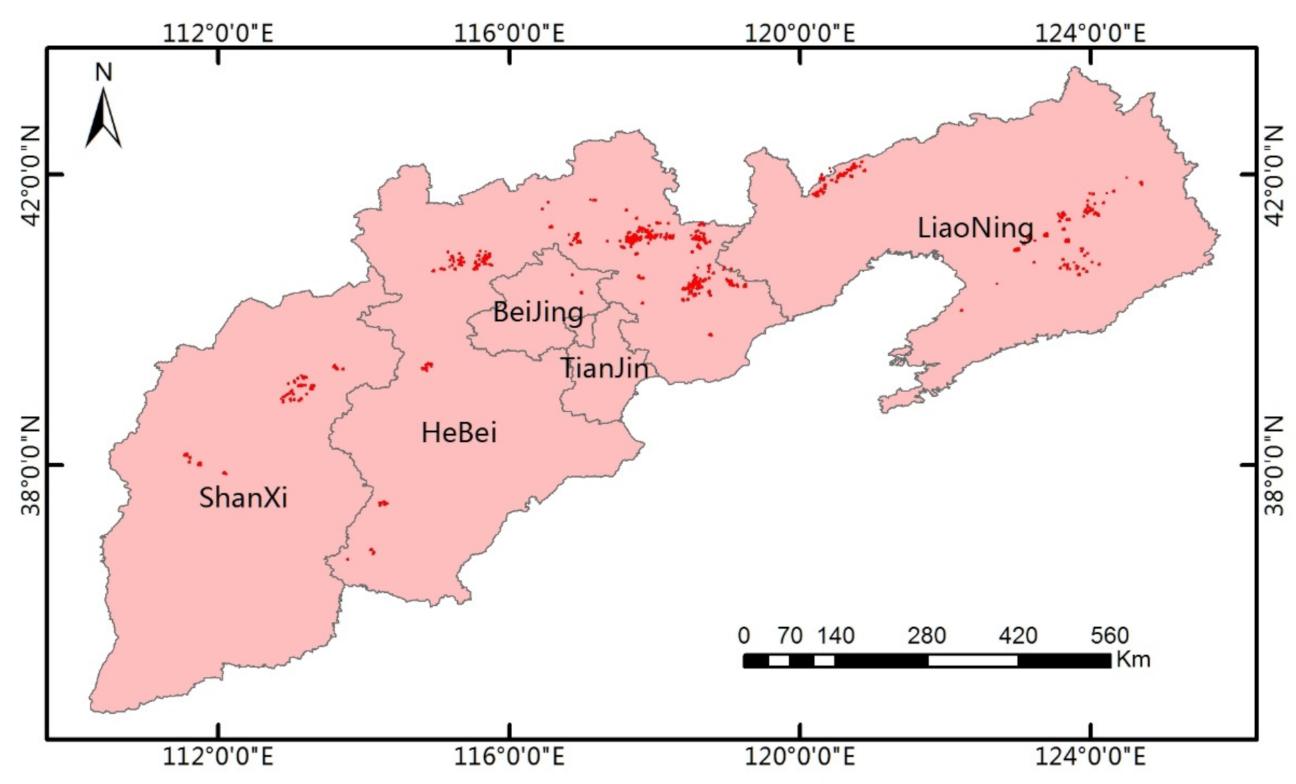
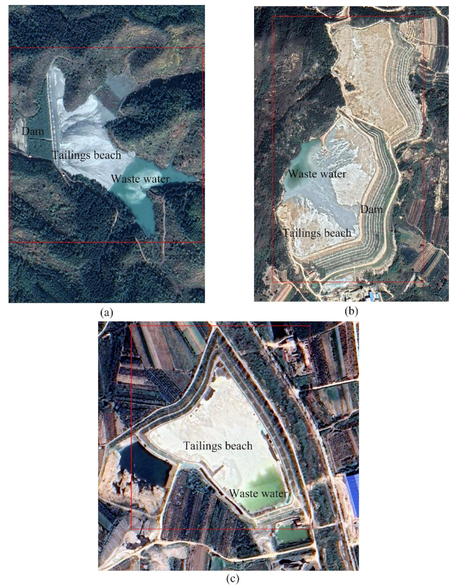
2.1. Sampling Data Generation

Hebei Province, Shanxi Province, and Liaoning Province in northern China, which have a large number of tailings ponds, were selected as the study area for sample labeling. By selecting tailings pond samples in a relatively large area, the limitation of sample specificity in small areas can be reduced to a certain extent, thereby enhancing the model’s generalization ability in large-scale applications. Based on GoogleEarth high-resolution remote sensing image data, a total of 1200 tailings ponds were labeled as sample data to train and test the models of interest. GoogleEarth high-resolution images have a data level of 18, a spatial resolution of 0.5 m, including three bands of red, green, and blue and 8-bit data bits. The geographical distribution of the tailings pond samples is shown in Figure 1.
The shape of tailings pond facilities on the ground is determined by the natural landform features as well as artificial and engineering features [35]. Due to the influence of topography and geomorphology, mineral resource mining, mining technology, operation scale, and other factors, tailings ponds can be classified into four types: cross-valley, hillside, stockpile, and cross-river [15]. Cross-valley tailings ponds are formed by building a dam at a valley mouth. Their main characteristics are a relatively short initial dam and a relatively long reservoir area (Figure 2a). Hillside tailings ponds are surrounded by a dam built at the foot of a mountain slope. Their main characteristics are a relatively long initial dam and a relatively short reservoir area (Figure 2b). Stockpile tailings ponds are formed by a dam at the periphery of a flat area. Their characteristics are a high engineering workload for the initial dam and subsequent dams of the tailings ponds and a relatively low tailings dam height (Figure 2c). Cross-river tailings ponds are formed by dams built to the upstream and downstream of the riverbed. Their main characteristics are a large upstream catchment area and a complex tailings pond and upstream drainage system. As cross-river tailings ponds are rarely distributed in China, the sample tailings ponds labeled in this study only included the other three types.
Based on the characteristics of the three types of tailings pond and their remote sensing image features, a total of 1200 tailings pond samples were labeled in this study, 80% of which were used as training samples, with the remaining 20% used as test samples. To improve sample labeling efficiency, the samples were first marked as the external polygon vector of the tailings pond. Thereafter, they were uniformly processed into an external rectangle, which was used as the final detection labeling target, based on the program. The red boxes in Figure 2 indicate the labeled ground truth bounding boxes. Due to computational limitations such as memory and GPU video memory, the remote sensing image data were sliced into image blocks of appropriate sizes then resampled before being input to the model to complete the calculation. According to a statistical analysis of the labeled tailings pond samples, their lengths and widths typically ranged from 60 m to 1300 m, and the resolution of the image data was 0.5 m. To ensure the integrity of tailings ponds in the image slices as much as possible, the image slice size was set to 2600 × 2600 pixels for slice processing in this study. An overlapping area of 512 pixels was set between the image slices, and after processing, image slices without tailings pond information were eliminated. Thus, a total of 1697 effective training slices and 429 test slices were finally generated. The sample set information is listed in Table 1.

2.2. Methodology

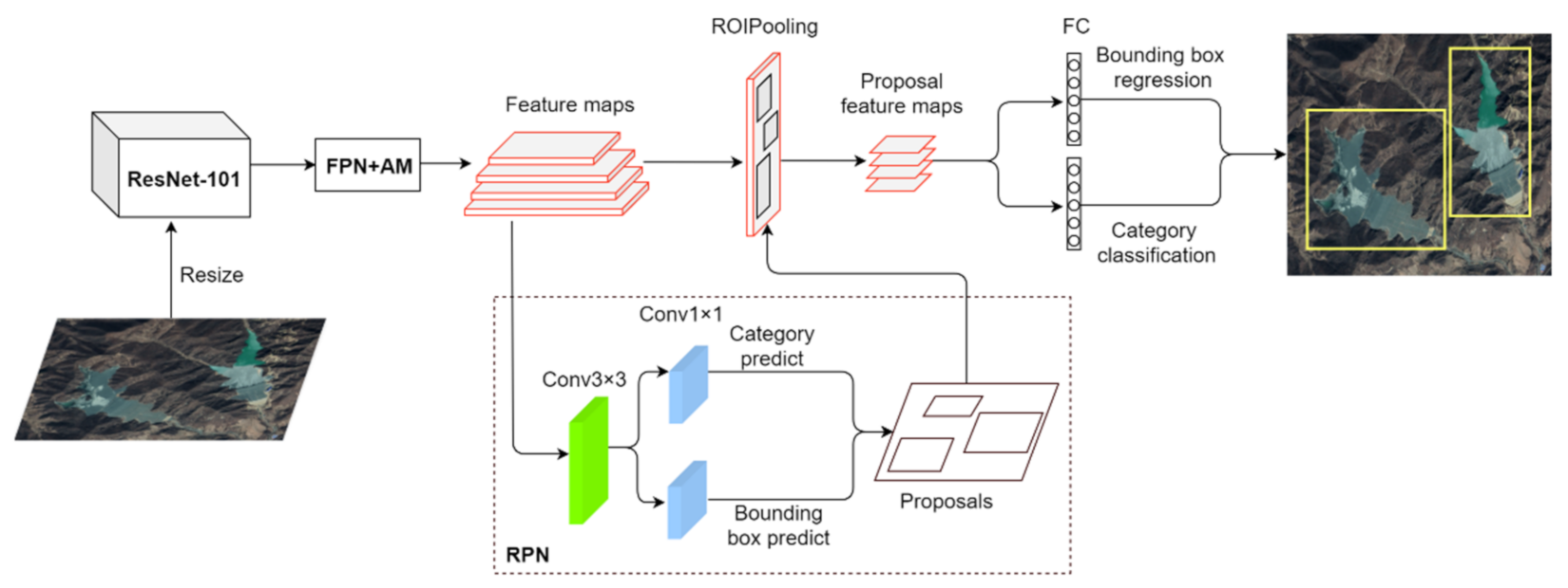
2.2.1. Proposed Optimized Method

Faster R-CNN is a classic deep learning-based target detection model in the field of computer vision [36], which exhibits relatively high recognition precision and efficiency for large target areas. With the continuous development of deep learning technology, there is still room for improving the precision of the Faster R-CNN model for the detection of tailings pond targets in high-resolution remote sensing images. In this study, an improved Faster R-CNN model was developed, whose structure is shown in Figure 3. First, after resize, the remote sensing image slices were input to ResNet-101 for feature extraction, and multilevel features were output. Second, the multilevel features were input into the feature pyramid network (FPN) [37] with the attention mechanism (AM) for feature fusion to generate multiscale feature maps with rich context information. Third, the feature map was input into the RPN to generate region proposals after predicting the category and bounding box. Fourth, the feature maps and region proposals were input into the ROIPooling layer to generate proposal feature maps. Finally, the proposal feature maps were sent to the subsequent fully connected layers (FC) to determine the target category and obtain the precise position of the target bounding box.
Compared with the Faster R-CNN, the proposed model exhibits the following improvements: (1) ResNet-101 was used as the feature extraction network to enhance the image feature extraction capability, and the FPN was adopted to perform feature fusion on the multilevel feature output from the ResNet-101 to obtain feature maps with rich semantic and location information; (2) the AM was adopted to improve the FPN. The contribution degrees of feature channels were recalibrated so that features with high contribution degrees were enhanced and features with low contribution degrees were suppressed, thereby further improving FPN performance; (3) the image slice size was set according to the statistical results of the tailings pond samples, where the integrity of the tailings ponds in the image slices was maintained as much as possible. In addition, the model input size with the highest precision was selected by conducting a comparison study.

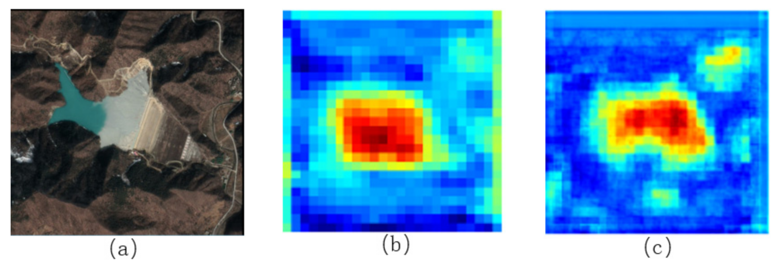
Attention Mechanism (AM)

The visual AM is a brain signal processing mechanism unique to human vision. In focus target areas, more attention resources will be allocated to obtain more detailed information, whereas information in other areas will be suppressed. Thus, high-value information can be acquired rapidly from a large amount of information, which greatly improves the information processing efficiency of the brain. Therefore, the AM has become an important concept in neural networks in recent years [38] as it can greatly improve network performance by focusing on only processing key information or information of interest among large amounts of input information. In normal cases, the feature layer extracted by a deep CNN is used, where each channel represents a different feature and also has a different contribution to network performance. The SENet [39] uses the AM to learn the contribution weight of each channel of the feature layer and automatically obtain the importance of each feature channel. According to the importance level, features with high contributions are then enhanced and those with low contributions are suppressed, thereby improving network performance. Therefore, the channel attention mechanism block was adopted in the design of the FPN in this study, which further improved the detection precision for tailings pond targets.
As shown in Figure 4, the input F of the channel attention mechanism block represents the feature map, H represents the height of the feature map, W represents the width of the feature map, and C represents the number of channels in the feature map. First, F was compressed into a 1 × 1 × C one-dimensional vector via Global Average Pooling (GAP). Each value in the vector has a global receptive field, characterizing the global distribution of responses on the feature channels. The two subsequent FC layers were used to model the correlations between channels. The first FC reduces the number of feature channels to C/r, where r is the scaling factor. After passing through the ReLu activation function, the second FC increases the number of feature channels back to the original C. Then, the Sigmoid function was used to obtain normalized weights representing the input feature contributions. Finally, through the Scale operation, the input feature was multiplied by the weight, which was extended to an equal dimension, to output the result A. Two FC layers can add more nonlinearity; however, if the scaling factor r of the first layer is too small, more parameters will be added and the calculation amount will increase; if it is too large, more features will be lost and network performance will be reduced. After balancing the amount of calculation and the network performance, the value of r was set to 4 in this study.

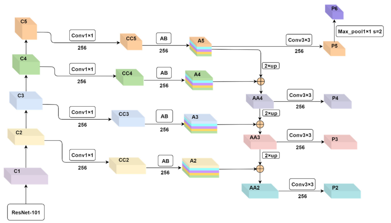
Proposed Feature Pyramid Network (FPN)

With the continuous development of deep learning technology in recent years, many convolutional neural networks have overcome the problems of gradient dispersion and gradient explosion caused by an increase in network depth to exhibit powerful feature extraction capabilities, for example, ResNet and DenseNet [40]. However, for single-scale features, although deep features have rich semantic information, there is a serious loss of location information. In target detection applications, location information is crucial. In comparison, shallow features have weak semantic information but are sensitive to location information. Therefore, the FPN was used to fuse deep and shallow multiscale features to fully exploit the feature semantics and location information, thereby further improving the network performance. As well as using ResNet-101 to improve the feature extraction capabilities, this study also adopted the channel attention mechanism block and designed an improved FPN, which fused features at different levels to obtain a more informative multiscale feature map, thereby greatly improving the detection precision of the model. The improved FPN is shown in Figure 5.
As shown in Figure 5, ResNet-101 was used as the feature extraction network in this study. C1, C2, C3, C4, and C5 in the network were used to extract different levels of features, with C2–C5 selected for feature fusion. The number of channels was 256, 512, 1024, and 2048, respectively. Combining features of different levels via the FPN requires the same number of feature channels. Therefore, the 1 × 1 convolution operation was used to reduce the dimensionality of C2–C5. The corresponding outputs were CC2–CC5, and the number of channels was 256. The channel attention mechanism block was used to calculate the contribution weight of each channel of CC2–CC5, which were redistributed according to their weight. Thus, the contributions of important feature channels were further enhanced. The corresponding outputs were A2–A5, and the number of channels remained unchanged at 256. When performing feature fusion via FPN, pixels corresponding to features of different levels were added. In addition to the same number of feature channels, the number of rows and columns in the feature layer must also be the same. Therefore, the nearest interpolation method was applied in this study to perform two-times upsampling on A5, A4, and A3. Subsequently, element-wise addition was performed with A4, A3, and A2, respectively, to complete the level-by-level feature fusion, where the output was AA2, AA3, and AA4 and the number of channels was 256. A 3 × 3 convolution operation was performed on A5, where the output was P5 and the number of channels was 256. Maximum pooling of 1 × 1 was performed on P5, the stride was set to 2, the output was P6, and the number of channels was 256. A 3 × 3 convolution operation was performed on AA2, AA3, and AA4, where the outputs were P2, P3, and P4 and the number of channels was 256. The feature map output by FPN was {P2, P3, P4, P5, P6}.

Region Proposal Network (RPN)

The most prominent contribution of Faster R-CNN is the RPN, which uses a CNN instead of the traditional selective search method to generate candidate regions, thereby significantly improving network speed and precision. RPN is used to generate region proposals. In this study, the multiscale feature maps {P2, P3, P4, P5, P6} output from the FPN were used to replace the single-scale feature map to generate region proposals. The areas of anchors for different scale features were set to {322, 642, 1282, 2562, 5122}, and the anchor aspect ratios were set to {1:2, 1:1, 2:1}.
In this study, feature maps input into ROIPooling with region proposals include {P2, P3, P4, P5}, rather than a single-scale feature map. In other words, the region proposal needs to slice the region proposal feature map from {P2, P3, P4, P5}. The following formula was used for region proposal to select the feature map with the most appropriate scale:
k = k 0 + log 2 ( w h / H )
where k represents the level of feature map corresponding to the region proposal, which is rounded off during calculation; k0 was set as the highest level of feature maps. In this study, there were four levels of feature maps and k0 was set to four; w and h represent the width and height of the region proposal, respectively, and H represents the model input height (the height and width are equal in this study) after performing resize processing on the image slices. This is a more reasonable approach because a large-size region proposal will correspond to a high-level feature map and generate the region proposal feature map, which can better detect large targets. Similarly, a small-size region proposal corresponds to a low-level feature map and generates the region proposal feature map, which can better detect small targets.

2.2.2. Accuracy Assessment

In the field of deep learning, precision and recall are the commonly used evaluation indicators for model performance [41]. When evaluating the target detection results, the ground truth bounding box (GT) is the true bounding box of the predicted target, whereas the predicted bounding box (PT) is the predicted bounding box of the predicted target. The area encompassed by both the predicted bounding box and the ground truth is denoted as the area of union, the intersection is denoted as the area of overlap, and the calculation formula of the intersection over union (IOU) is as follows:
IOU = Area   of   Overlap Area   of   Union
where TP (true positive) refers to the number of detection boxes with correct detection results and an IOU > 0.5; FP(false positive) refers to the number of detection boxes with incorrect detection results and an IOU ≤ 0.5; and FN (false negative) refers to the number of GTs that are not detected. The model evaluation indicators used in this study were precision and recall. Precision refers to the ratio of the number of correct detection boxes to the total number of detection boxes, whereas recall refers to the ratio of the number of correct detection boxes to the total number of true bounding boxes. Their corresponding calculation formulas are as follows:
Precision = TP TP + FP
Recall = TP TP + FN
The average precision (AP) of the target, precision-recall curve (PRC), and mean average precision (mAP) are three common indicators widely applied to evaluate the performance of object detection methods [42]. AP is typically the area under the PRC and mAP is the average value of AP values for all classes; the larger the mAP value, the better the object detection performance. As this study only detects one target, namely a tailings pond, AP was used as the main model evaluation indicator, with the recall and time consumption of a single iteration used as reference indicators.

2.2.3. Loss Function

The formula for the calculation of the Loss Function can be expressed as follows [24]:
L p i , t i = 1 N c l s i L c l s p i , p i * + α 1 N r e g i p i * L r e g t i , t i *
where Ncls represents the number of anchors in the mini batch, Nreg represents the number of anchor locations, and α represents the weight balance parameter, which was set to 10 in this study, and i represents the index of an anchor in a mini batch.
Furthermore, p i represents the predictive classification probability of the anchor. Specifically, when the anchor was positive, p i * = 1, and when it was negative, p i *   = 0. Moreover, anchors that met the following two conditions were considered positive: (1) the anchor has the highest intersection-over-union (IOU) overlap with a ground truth box; or (2) the IOU overlap of the anchor with the ground truth box is > 0.7. Conversely, when the IOU overlap of the anchor with any ground-truth box was < 0.3, the anchor was considered negative. Anchors that were neither positive nor negative were not included in the training.
L c l s p i , p i * = l o g p i p i * + 1 p i 1 p i *
L r e g t i , t i * = i x , y , w , h S m o o t h L 1 t i t i *
S m o o t h L 1 x = 0.5 x 2 ,   i f x < 1 x 0.5 ,   o t h e r w i s e
For the bounding box regression, we adopted the parameterization of four coordinates, defined as follows:
t x = x x a w a ,   t y = y y a h a
t w = log w w a ,   t h = log h h a
t x * = x * x a w a ,   t y * = y * y a h a
t w * = log w * w a ,   t h * = log h * h a
where x and y represent the coordinates of the center of the bounding box, and w and h represent the width and height of the bounding box, respectively. Furthermore, x, xa, and x* correspond to the predicted box, anchor box, and ground truth box, respectively, similar to y, w, and h.

2.2.4. Training and Optimization

As Faster R-CNN was employed as the baseline network, the hyperparameters were set according to Faster R-CNN. This study adopts the transfer learning strategy, the base network was ResNet 101, which was initialized with its pretrained weights on ImageNet. All new layers were initialized with kaimingnormal. The network was trained using a 64-bit Ubuntu20.04LTs operating system and a NVIDIA GeForce GTX3080, using Xeon E5 CPU and CUDA version 11.1. The model trained 70 epochs of the training set. Stochastic gradient descent was used as the optimizer, the initial learning rate of the model was set to 0.02, momentum was set to 0.9, weight_decay was set to 0.0001, and the batch size was set to 2. The hyperparameters settings are listed in Table 2.

3. Results and Discussion

In this study, the channel attention mechanism block was adopted to design an improved FPN on the basis of the Faster R-CNN model. The improved model exhibits a significant improvement in the detection performance of tailings pond targets compared to the Faster R-CNN model. Based on the data set of tailings pond samples constructed in this study, the model input size greatly affected the detection precision; the results show that when resize = [800, 800], the detection precision of tailings pond is the highest and both the AP and recall of tailings pond detection increased significantly in the improved model, by 5.6% and 10.9% to reach 85.7% and 62.9%, respectively. The results above are analyzed in detail in the following sections.

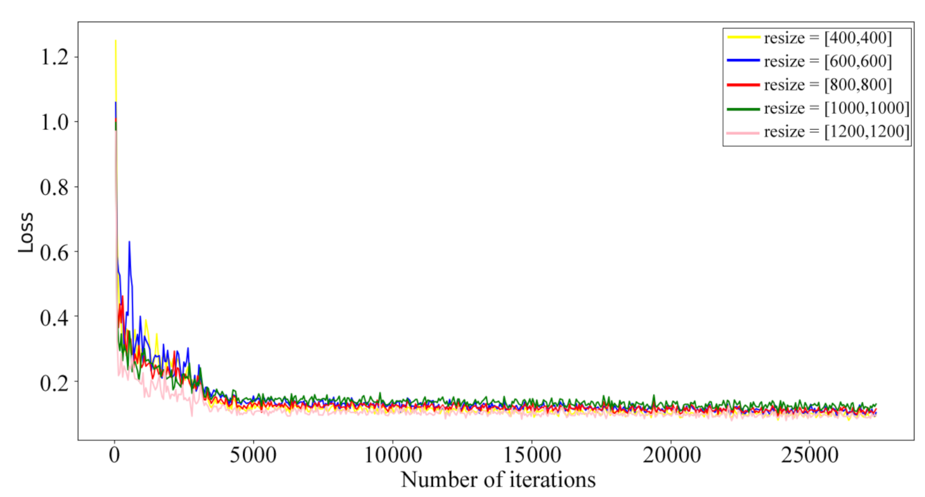
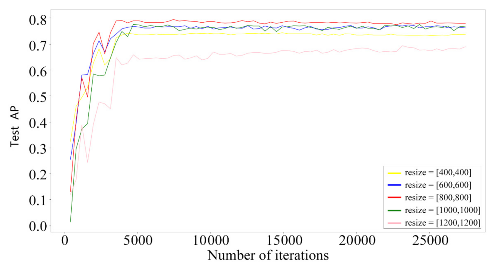
3.1. Effect of Different Input Sizes

Based on the Faster R-CNN model, the model detection precision was compared for different model input sizes. It was assumed that the size of the input image slice was [W, H, C], where W, H, and C are the width of the slice, height of the slice, and number of channels in the slice, respectively. The size of the image slice in the tailings pond sample data set was [2600, 2600, 3]. According to the bilinear interpolation resampling method, the image slices were used as the model input after resize processing in W and H dimensions, during which the number of channels C remained unchanged. After downsampling, the sizes of W and H were set to resize = [400, 400], [600, 600], [800, 800], [1000, 1000], [1200, 1200], totaling five sizes. The resize size with the highest precision was selected as the model input size.
According to the training loss curves in Figure 6, the trends of the model loss curves are approximately the same for different resize sizes, the loss values are similar, and all values converge well. However, the test precision curves of the model (Figure 7) indicate that the model exhibits the strongest generalization ability and maintains the highest test precision when resize = [800, 800]. The model evaluation indicator results for different resize sizes are listed in Table 3. When resize = [800, 800], the model AP reaches a maximum of 80.1%. Compared with resize = [600, 600], the recall is slightly smaller (1%) but the AP is 2.8% higher. However, as the resize size either increases or decreases, both the AP and recall of the model decrease, especially for resize = [1200, 1200], where AP and recall drop to their minimum values of 69.3% and 41.8%, respectively. According to the time consumption of a single iteration, the calculation amount of the model increases as the resize size increases, resulting in a longer calculation time. Compared to resize = [400, 400], when resize = [800, 800], the iteration time only increases slightly (0.081 s) but the AP increases by 5.8% and the recall increases by 0.2%. Overall, a resize value of [800, 800] generates optimal model performance.

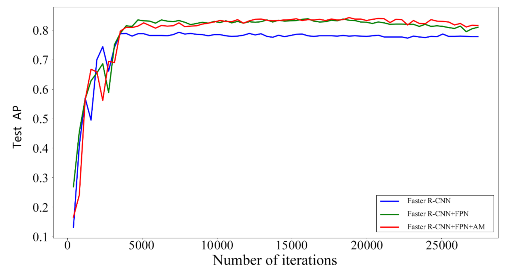
3.2. Analysis of Model Improvement Results

The optimal model input size was selected through a comparison study. After obtaining the optimal performance using the Faster R-CNN model, further improvements were made to the model. First, the FPN was introduced, and the corresponding model was represented by Faster R-CNN + FPN. Then, the channel attention mechanism block was adopted to further improve the FPN, and the corresponding model was represented by Faster R-CNN + FPN + AB. According to the loss curves, all models exhibit good convergence (Figure 8). In addition, after improving the model with FPN and AB, the model exhibits the best convergence and the lowest loss value. Furthermore, according to the model test precision curves, the improved final model has the highest test precision (Figure 9). The evaluation indicator results of each model are listed in Table 4, which show that both the AP and recall indicators of the model are greatly improved by using the FPN, increasing by 4.2% and 10.6%, respectively. This indicates that the model detection capability is significantly improved by combining features of different scales, although the increased calculation amount and number of parameters results in an increase in the time required for a single iteration. After further adoption of AB, both the AP and recall of the model increase by 1.4% and 0.3%, respectively, whereas the time required for a single iteration only increases by 0.006 s. Thus, through application of the channel attention mechanism, the detection performance is significantly improved and the calculation amount and iteration time are increased only by a small amount. Compared with the Faster R-CNN model, the AP and recall of the final improved model increase by 5.6% and 10.9%, reaching 85.7% and 62.9%, respectively.
In summary, the improved model exhibits a significant increase in the detection precision of tailings ponds compared to Faster R-CNN, as well as more accurate location positioning. Furthermore, cases of missed detection and false detection are also reduced.
As shown in Figure 10, (a) is the image of tailings pond, (b) is the feature heat map extracted by the Faster R-CNN model, and (c) is the feature heat map extracted by the improved model. The characteristics of tailings pond extracted from the improved model are obviously improved in terms of shape and contour. As shown in Figure 11, Figure 12 and Figure 13, the green bounding box represents the tailings pond predicted by the model. Figure 11a is the prediction result of Faster R-CNN, which has a prediction score of 0.97. However, an error appears in the predicted bounding box position, where the upper right corner of the tailings pond is not included. Figure 11b is the prediction result of the improved model, where the score is increased to 1.0 and the accuracy of the bounding box position is significantly improved. Moreover, the red arrow in Figure 12a indicates a non-detected tailings pond, whereas the tailings pond is accurately detected by the improved model. Additionally, the improved model exhibits a significantly better score and location accuracy for other detected tailings pond targets than Faster R-CNN. Finally, as shown in Figure 13, the improved model also avoids the false detection of tailings pond by Faster R-CNN.

4. Conclusions

This study improved the Faster R-CNN model and proposed an intelligent identification method for tailings ponds based on high-resolution remote sensing images, which significantly improves the detection precision of tailings pond targets. Based on the data set of tailings pond samples constructed in this study, it was found that the model input size greatly affected the detection precision and the results show that when resize = [800, 800], the detection precision of tailings pond is the highest. To improve the image feature extraction capabilities of the model, using ResNet-101 as the feature extraction network, the channel attention mechanism block was adopted and an improved FPN was designed. This improved model recalibrated the contribution degrees of the feature channels while fusing features at different levels, thereby enhancing features with high contribution degrees and suppressing features with low contribution degrees. The test results show that both the AP and recall of tailings pond detection increased significantly in the improved model, by 5.6% and 10.9% to reach 85.7% and 62.9%, respectively. Considering the rapid growth in high-resolution remote sensing images, this method has important applications for large-scale, high-precision, and intelligent identification of tailings ponds, which will greatly improve the decision-making efficiency of tailings pond management.

Author Contributions

Conceptualization, G.L. and D.Y.; methodology, D.Y.; software, D.Y and K.L.; validation, D.Y., X.L. and H.Z.; formal analysis, M.C.; investigation, H.L.; resources, F.Z.; data curation, X.L.; writing—original draft preparation, D.Y.; writing—review and editing, G.L. and D.Y.; visualization, D.Y.; supervision, G.L.; project administration, G.L.; funding acquisition, G.L. and H.Z. All authors have read and agreed to the published version of the manuscript.

Funding

This research was funded by National Key Research and Development Program of China from Ministry of Science and Technology, grant number 2016YFB0501504; the National Natural Science Foundation of China, grant number 41771397.

Acknowledgments

The authors would like to thank the editors and the anonymous reviewers for their helpful suggestions.

Conflicts of Interest

The authors declare no conflict of interest.

Abbreviations

ILSVRCImageNet large-scale visual recognition challenge
CNNconvolutional neural network
FCfully connected layers
RPNregion proposal network
FPNfeature pyramid network
AMattention mechanism
ABchannel attention mechanism block
GTground truth bounding box
PTpredicted bounding box
IOUintersection over union
APaverage precision
mAPmean average precision
PRCprecision-recall curve

References

  1. Wang, T.; Hou, K.P.; Guo, Z.S.; Zhang, C.L. Application of analytic hierarchy process to tailings pond safety operation analysis. Rock Soil Mech. 2008, 29, 680–687. [Google Scholar]
  2. Xiao, R.; Lv, J.; Fu, Z.; Sheng, W.; Xiong, W.; Shi, Y.; Cao, F.; Yu, Q. The Application of Remote Sensing in the Environmental Risk Monitoring of Tailings pond in Zhangjiakou City, China. Remote Sens. Technol. Appl. 2014, 29, 100–105. [Google Scholar]
  3. Santamarina, J.C.; Torres-Cruz, L.A.; Bachus, R.C. Why coal ash and tailings dam disasters occur. Science 2019, 364, 526. [Google Scholar] [CrossRef] [PubMed]
  4. Jie, L. Remote Sensing Research and Application of Tailings Pond–A Case Study on the Tailings Pond in Hebei Province; China University of Geosciences: Beijing, China, 2014. [Google Scholar]
  5. Gao, Y.; Hou, J.; Chu, Y.; Guo, Y. Remote sensing monitoring of tailings ponds based on the latest domestic satellite data. J. Heilongjiang Inst. Technol. 2019, 33, 26–29. [Google Scholar]
  6. Tan, Q.L.; Shao, Y. Application of remote sensing technology to environmental pollution monitoring. Remote. Sens. Technol. Appl. 2000, 15, 246–251. [Google Scholar]
  7. Dai, Q.W.; Yang, Z.Z. Application of remote sensing technology to environment monitoring. West. Explor. Eng. 2007, 4, 209–210. [Google Scholar]
  8. Wang, Q. The progress and challenges of satellite remote sensing technology applications in the field of environmental protection. Environ. Monit. China 2009, 25, 53–56. [Google Scholar]
  9. Liu, W.T.; Zhang, Z.; Peng, Y. Application of TM image in monitoring the water quality of tailing reservoir. Min. Res. Dev. 2010, 30, 90–92. [Google Scholar]
  10. Zhao, Y.M. Moniter Tailings based on 3S Technology to Tower Mountain in Shanxi Province. Master’s Thesis, China University of Geoscience, Beijing, China, 2011; pp. 1–46. [Google Scholar]
  11. Hao, L.; Zhang, Z.; Yang, X. Mine tailing extraction indexes and model using remote-sensing images in southeast Hubei Province. Environ. Earth Sci. 2019, 78, 493. [Google Scholar] [CrossRef] [Green Version]
  12. Ma, B.; Chen, Y.; Zhang, S.; Li, X. Remote sensing extraction method of tailings ponds in ultra-low-grade iron mining area based on spectral characteristics and texture entropy. Entropy 2018, 20, 345. [Google Scholar] [CrossRef] [Green Version]
  13. Xiao, R.; Shen, W.; Fu, Z.; Shi, Y.; Xiong, W.; Cao, F. The application of remote sensing in the environmental risk monitoring of tailings pond: A case study in Zhangjiakou area of China. SPIE Proc. 2012, 8538. [Google Scholar]
  14. Riaza, A.; Buzzi, J.; García-Meléndez, E.; Vázquez, I.; Bellido, E.; Carrère, V.; Müller, A. Pyrite mine waste and water mapping using Hymap and Hyperion hyperspectral data. Environ. Earth Sci. 2012, 66, 1957–1971. [Google Scholar] [CrossRef]
  15. Li, Q.; Chen, Z.; Zhang, B.; Li, B.; Lu, K.; Lu, L.; Guo, H. Detection of tailings dams using high-resolution satellite imagery and a single shot multibox detector in the Jing–Jin–Ji Region, China. Remote. Sens. 2020, 12, 2626. [Google Scholar] [CrossRef]
  16. Liu, W.; Anguelov, D.; Erhan, D.; Szegedy, C.; Reed, S.; Fu, C.Y.; Berg, A.C. Ssd: Single shot multibox detector. In Proceedings of the European Conference on Computer Vision, Amsterdam, The Netherlands, 8–16 October 2016; pp. 21–37. [Google Scholar]
  17. Krizhevsky, A.; Sutskever, I.; Hinton, G.E. ImageNet classification with deep convolutional neural networks. In Advances in Neural Information Processing Systems; Pereira, F., Burges, C.J.C., Bottou, L., Weinberger, K.Q., Eds.; Curran Associates, Inc.: New York, NY, USA, 2012; pp. 1106–1114. [Google Scholar]
  18. Simonyan, K.; Zisserman, A. Very deep convolutional networks for large-scale image recognition. arXiv 2014, arXiv:1409.1556. [Google Scholar]
  19. He, K.; Zhang, X.; Ren, S.; Sun, J. Deep Residual Learning for Image Recognition. In Proceedings of the IEEE Conference on Computer Vision and Pattern Recognition, Las Vegas, NV, USA, 27–30 June 2016. [Google Scholar]
  20. Huang, G.; Liu, Z.; van der Maarten, L.; Weinberger, K.Q. Densely connected convolutional networks. arXiv 2016, arXiv:1608.06993. [Google Scholar]
  21. Wu, X.; Sahoo, D.; Hoi, S.C.H. Recent advances in deep learning for object detection. Neurocomputing 2020, 396, 39–64. [Google Scholar] [CrossRef] [Green Version]
  22. Girshick, R.; Donahue, J.; Darrell, T.; Malik, J. Rich Feature Hierarchies for Accurate Object Detection and Semantic Segmentation. In Proceedings of the 2014 IEEE Conference on Computer Vision and Pattern Recognition, Columbus, OH, USA, 23–28 June 2014; pp. 580–587. [Google Scholar]
  23. Girshick, R. Fast R-CNN. In Proceedings of the IEEE International Conference on Computer Vision, Santiago, Chile, 7–13 December 2015; pp. 1440–1448. [Google Scholar]
  24. Ren, S.; He, K.; Girshick, R.; Sun, J. Faster R-CNN: Towards Real-Time Object Detection with Region Proposal Networks. In Proceedings of the Advances in Neural Information Processing Systems, Montreal, QC, Canada, 7–12 December 2015; MIT Press: Cambridge, MA, USA, 2016; pp. 91–99. [Google Scholar]
  25. Redmon, J.; Divvala, S.; Girshick, R.; Farhadi, A. You Only Look Once: Unified, Real-Time Object Detection. In Proceedings of the 2016 IEEE Conference on Computer Vision and Pattern Recognition, Las Vegas, NV, USA, 27–30 June 2016; pp. 779–788. [Google Scholar]
  26. Redmon, J.; Farhadi, A. Yolov3: An incremental improvement. arXiv 2018, arXiv:1804.02767. [Google Scholar]
  27. Redmon, J.; Farhadi, A. YOLO9000: Better, Faster, Stronger. In Proceedings of the IEEE Conference on Computer Vision and Pattern Recognition (CVPR 2017), Honolulu, HI, USA, 21–26 July 2017; pp. 7263–7271. [Google Scholar]
  28. Li, Y.; Huang, Q.; Pei, X.; Jiao, L.; Ronghua. RADet: Refine feature pyramid network and multi-layer attention network for arbitrary-oriented object detection of remote sensing images. Remote Sens. 2020, 12, 389. [Google Scholar] [CrossRef] [Green Version]
  29. He, K.; Gkioxari, G.; Dollár, P.; Girshick, R. Mask r-cnn. In Proceedings of the 2017 IEEE International Conference on Computer Vision, Venice, Italy, 22–29 October 2017; pp. 2961–2969. [Google Scholar]
  30. Li, Y.; Xu, W.; Chen, H.; Jiang, J.; Li, X. A Novel Framework Based on Mask R-CNN and Histogram Thresholding for Scalable Segmentation of New and Old Rural Buildings. Remote. Sens. 2021, 13, 1070. [Google Scholar]
  31. Bhuiyan, M.A.E.; Witharana, C.; Liljedahl, A.K. Use of Very High Spatial Resolution Commercial Satellite Imagery and Deep Learning to Automatically Map Ice-Wedge Polygons across Tundra Vegetation Types. J. Imaging 2020, 6, 137. [Google Scholar] [CrossRef]
  32. Zhao, K.; Kang, J.; Jung, J.; Sohn, G. Building extraction from satellite images using mask R-CNN with building boundary regularization. In Proceedings of the IEEE Conference on Computer Vision and Pattern Recognition Workshops, Salt Lake City, UT, USA, 18–22 June 2018. [Google Scholar]
  33. Bai, T.; Pang, Y.; Wang, J.; Han, K.; Luo, J.; Wang, H.; Lin, J.; Wu, J.; Zhang, H. An Optimized Faster R-CNN Method Based on DRNet and RoI Align for Building Detection in Remote Sensing Images. Remote Sens. 2020, 12, 762. [Google Scholar] [CrossRef] [Green Version]
  34. Liu, Y.; Cen, C.; Che, Y.; Ke, R.; Ma, Y.; Ma, Y. Detection of Maize Tassels from UAV RGB Imagery with Faster R-CNN. Remote Sens. 2020, 12, 338. [Google Scholar] [CrossRef] [Green Version]
  35. Yu, G.; Song, C.; Pan, Y.; Li, L.; Li, R.; Lu, S. Review of new progress in tailing dam safety in foreign research and current state with development trend in China. Chin. J. Rock Mech. Eng. 2014, 33, 3238–3248. [Google Scholar]
  36. Ren, S.; He, K.; Girshick, R.; Sun, J. Faster R-CNN: Towards real-time object detection with region proposal networks. arXiv 2015, arXiv:1506.01497. [Google Scholar] [CrossRef] [Green Version]
  37. Lin, T.Y.; Dollar, P.; Girshick, R.; He, H.; Hariharan, B.; Belongie, S. Feature pyramid networks for object detection. arXiv 2017, arXiv:1612.03144. [Google Scholar]
  38. Chaudhari, S.; Mithal, V.; Polatkan, G.; Ramanath, R. An attentive survey of attention models. arXiv 2020, arXiv:1904.02874. [Google Scholar]
  39. Hu, J.; Shen, L.; Sun, G. Squeeze-and-excitation Networks. In Proceedings of the 2018 IEEE Conference on Computer Vision and Pattern Recognition, Salt Lake City, UT, USA, 18–23 June 2018; pp. 7132–7141. [Google Scholar]
  40. Huang, G.; Liu, Z.; Van Der Maaten, L.; Weinberger, K.Q. Densely Connected Convolutional Networks. In Proceedings of the 2017 IEEE Conference on Computer Vision and Pattern Recognition, Honolulu, HI, USA, 21–26 July 2017. [Google Scholar]
  41. Buckland, M.; Gey, F. The relationship between Recall and Precision. J. Am. Soc. Inf. Sci. 1994, 45, 12–19. [Google Scholar] [CrossRef]
  42. Han, J.; Zhou, P.; Zhang, D.; Cheng, G.; Guo, L.; Liu, Z.; Bu, S.; Wu, J. Efficient, simultaneous detection of multi-class geospatial targets based on visual saliency modeling and discriminative learning of sparse coding. ISPRS J. Photogramm. Remote Sens. 2014, 89, 37–48. [Google Scholar] [CrossRef]
Figure 1. Geographical distribution map of tailings pond samples.
Remotesensing 13 02052 g001
Figure 2. Remote sensing image of sample tailings pond features, with the ground truth bounding boxes shown in red: (a) cross-valley type, (b) hillside type, and (c) stockpile type.
Remotesensing 13 02052 g002
Figure 3. Proposed optimized network structure.
Remotesensing 13 02052 g003
Figure 4. Schematic of the channel attention mechanism block.
Remotesensing 13 02052 g004
Figure 5. Feature pyramid network (FPN) structure. AB represents the channel attention mechanism block, 2 × up represents two-times upsampling, 256 represents the number of output channels, and Remotesensing 13 02052 i001 represents element-wise addition.
Remotesensing 13 02052 g005
Figure 6. Training loss curves for different resize sizes.
Remotesensing 13 02052 g006
Figure 7. Test precision curves for different resize sizes.
Remotesensing 13 02052 g007
Figure 8. Loss curves of different network models.
Remotesensing 13 02052 g008
Figure 9. Test precision curves of different network models.
Remotesensing 13 02052 g009
Figure 10. Feature extraction capability improved after model improvement: (a) the image of tailings pond, (b) feature heat map of Faster R-CNN, and (c) feature heat map of the improved model.
Remotesensing 13 02052 g010
Figure 11. Increased position prediction accuracy after model improvement: (a) prediction results of Faster R-CNN and (b) prediction results of the improved model.
Remotesensing 13 02052 g011aRemotesensing 13 02052 g011b
Figure 12. Improvement in missed detections of tailings ponds after model improvement: (a) prediction results of Faster R-CNN, (b) prediction results of the improved model, and the red arrow indicates a non-detected tailings pond.
Remotesensing 13 02052 g012
Figure 13. Improvement in false detections of tailings ponds after model improvement: (a) prediction results of Faster R-CNN, (b) prediction results of the improved model, and the red arrow indicates a false detected tailings pond.
Remotesensing 13 02052 g013
Table 1. The sample set information.
Sample SetSpatial Resolution (m)Size (Pixels)Slices Number
Train set0.52600 × 26001697
Test set0.52600 × 2600429
Table 2. Table for hyperparameters settings.
HyperparameterLearning RateMomentumWeight_DecayBatch Size
Value0.020.90.00012
Table 3. Test results for different resize sizes.
ResizeAP (%)Recall (%)Iteration Time (s)
[400, 400]74.351.80.105
[600, 600]77.353.00.128
[800, 800]80.152.00.186
[1000, 1000]77.547.30.259
[1200, 1200]69.341.80.345
Table 4. Test results of different network models.
NetworkAP (%)Recall (%)Iteration Time (s)
Faster R-CNN80.152.00.186
Faster R-CNN + FPN84.362.60.273
Faster R-CNN + FPN + AB85.762.90.279
Publisher’s Note: MDPI stays neutral with regard to jurisdictional claims in published maps and institutional affiliations.

