Article

A Novel Approach to Obtain Diurnal Variation of Bio-Optical Properties in Moving Water Parcel Using Integrated Drifting Buoy and GOCI Data: A Case Study in Yellow and East China Seas

1
Ocean College, Zhejiang University, Zhoushan 316021, China
2
State Key Laboratory of Satellite Ocean Environment Dynamics, Second Institute of Oceanography, Ministry of Natural Resources, Hangzhou 310012, China
3
Southern Marine Science and Engineering Guangdong Laboratory (Guangzhou), Guangzhou 511458, China
4
School of Oceanography, Shanghai JiaoTong University, Shanghai 200030, China
*
Author to whom correspondence should be addressed.
Remote Sens. 2021, 13(11), 2115; https://0-doi-org.brum.beds.ac.uk/10.3390/rs13112115
Submission received: 8 April 2021 / Revised: 16 May 2021 / Accepted: 17 May 2021 / Published: 28 May 2021
(This article belongs to the Special Issue Seawater Bio-Optical Characteristics from Satellite Ocean Color Data)

Abstract

:
Ocean processes that can influence rapidly changing ocean color include water-mass movement and bio-optical property changes in the water parcel. Traditionally, diurnal variability of bio-optical properties relies on daily time series at fixed locations by satellite sensors or in situ observations. There is a lack of an effective way to observe diurnal variation of bio-optical properties in a moving water parcel on a large scale. In this paper, we propose a new method to acquire diurnal variation of bio-optical properties in a moving water parcel. The novel approach integrates drifting buoy data and GOCI data. The movement of surface current was tracked by a drifting buoy, and its spatiotemporally matching bio-optical properties were obtained via the GOCI data. The results in the Yellow and East China seas during the summers of 2012 and 2013 show that the variation of time series following the movement of water parcel was obviously different from that obtained at fixed locations. The hourly differences of the former are 15.7% and 16.3% smaller than those of the latter for Chl a and total suspended sediment (TSS), respectively. The value of ag440 was more stable within the moving water parcel than in the fixed location. Our approach provides a simple and feasible way for observing diurnal variability of bio-optical properties in a moving surface water parcel.

Graphical Abstract

1. Introduction

Understanding the dynamics of bio-optical properties in coastal systems and marginal seas is important for marine ecological environment monitoring. The variability of in-water bio-optical properties has been shown to be associated with specific environmental and biological conditions [1,2]. On the diurnal time scale, physical factors influencing such variability include tides, fronts, river discharge, ocean circulation, wind-driven mixing, etc. [3]. The bio-optical properties of water mass change along with the growth and decay of phytoplankton blooms, upwelling and downwelling, particle settling, and resuspension events [4,5]. These ocean processes can influence rapidly changing ocean color on the order of hours in different regions. In addition, biological, photochemical, and biogeochemical processes are regulated by the variation in solar radiation.
Remote sensing-based analysis on diurnal bio-optical variation of surface sea water is affected by the frequency of observations [6,7,8]. Satellite ocean color products from polar orbiting satellites (such as MODIS, SeaWiFS, MERIS, VIIRS, and so on) collect imagery on a daily time scale, and typically cannot be used to identify diurnal processes. Even multiple orbits combined can only capture limited diurnal variability [9,10]. The Geostationary Ocean Color Imager (GOCI) is the first geostationary orbit ocean color satellite sensor by the Korea Ocean Satellite Center (KOSC) [11], which provides possibly eight-time measurements in a day. Such data can play an important role in observing and estimating dynamic ocean environmental fields, and to reveal the diurnal variability in the ecosystem around the Northeast Asian sea region [12,13,14]. Ocean color produced by the GOCI has been shown to be useful in retrieving the total suspended sediment (TSS) concentration in the Yellow Sea (YS) [15], daily changes of colored dissolved organic material (CDOM) absorption coefficients at 440 nm (ag440) in the Yangtze River Estuary [16], and chlorophyll a (Chl a) in the East China Sea (ECS) [17].
Studies showed that with restriction to the time difference within one-hour between GOCI and in situ measurements, the mean ratios of normalized water-leaving radiance (nLw) at 490, 555, and 660 nm are 1.178, 1.073, and 1.098, respectively [18]. Then, the standard YOC (Yellow Sea Large Marine Ecosystem Ocean Color Project) algorithms are adopted to retrieve bio-optical properties from satellite data, such as Chl a, TSS, and ag440. It was reported that R2 of Chl a and TSS are 0.84 and 0.92, respectively [19,20]. Some validations and applications [21] indicated that the remote sensing reflectance retrieved by the KOSC algorithm has acceptable agreement with that of in situ observations, with R2 of 0.82 (490 nm) and 0.85 (555 nm). Despite the fact that the absolute value of Chl a can be overestimated at high TSS [13], the GOCI Chl a is still useful for understanding the variation and pattern in spatial distribution [22]. In addition, GOCI’s ocean color data were utilized to monitor hourly variability of turbidity and harmful algal bloom (HAB) [16,17,18,23,24,25]. However, most case studies on the diurnal variation of ocean color were based on time series analysis of remote sensing data at fixed locations [26,27,28]. On the other hand, GOCI’s ocean color data can be used to characterize and quantify surface currents [29], mesoscale eddies [30], and sub-mesoscale turbulence [31].
Ocean currents are critical for marine physical and biogeochemical processes [32]. The variability of bio-optical properties following surface currents has been observed by one drifter, which was equipped with bio-optical sensors and an automated water sampler [33]. Such drifter is expensive and difficult to operate. Actually, the above-mentioned drifter has two main functions: to follow the movement of water mass, and to measure variables. Recent surface drifting buoys have been widely used as a Lagrangian tracer [34] in maritime research due to their advantages, such as small size, low cost, and so on (e.g., [28,35]). The growing data from location-tracked drifters should become valuable for global and regional studies of small-scale processes in the ocean (e.g., [36]). However, surface drifting buoys carry limited information, and can only observe the movement trend of water mass without detailed characteristic parameters of the water parcel.
Ocean processes that can influence rapidly changing ocean color include intersection between the advection of water mass and the changes of bio-optical properties in the water parcel. There is a lack of an effective way to observe the diurnal variation of bio-optical properties in a moving water parcel. To examine the diurnal variation of bio-optical properties of the current, we developed a new approach to explore the trajectory of a moving water parcel and its changing bio-optical properties by combining the information of drifting buoys and GOCI observations. Instead of using a drifter similar to that described in [33], which was equipped with bio-optical sensors and an automated water sampler, we used Davis’s drogue drifter [34] to do the same, namely, following a particular water parcel. Meanwhile, the measurement of Abbott’s drifter [35] is replaced by that from satellite sensors. We utilized observations of the satellite (GOCI) as a proxy for measurements from bio-optical sensors affixed to a drifter, knowing that the algorithms used to derive these bio-optical properties from water-leaving reflectance include uncertainties that may not be quantified for all the water types sampled. Then, we conducted a case study to illustrate the difference between the time series at a fixed location and the time series following the water parcel; the latter combine buoy’s spatiotemporal data and GOCI-derived bio-optical properties. The remainder of this article is arranged as follows. The proposed methodology and dataset are described in Section 2. Main results and discussion are given in Section 3 and Section 4, respectively. Conclusions are provided in Section 5.

2. Materials and Methods

2.1. The Proposed Method

Typical research on diurnal variation of bio-optical properties is based on observing and/or sampling water at a fixed location. However, water sampling parameters at a fixed location change with time; and the change may be quite obvious, even during a single day. Hence, we propose a new method to construct a time series of bio-optical properties for moving surface water by integrating the data from drifting buoys and GOCI. The results are then compared with those from traditional fixed-location observations. The whole procedure (Figure 1) includes four modules: drifter data resampling, GOCI data processing, spatiotemporal matching, and time series construction and analysis.
First, we acquired the spatiotemporal information representing the movement of surface water collected by drifting buoys. The surface drifting buoy (Figure 2) is similar to Davis’s drogue drifter [34]; it provides drifter location with O (100 m) errors at non-uniform temporal interval, with an average sampling interval of 1.0 h. The surface float’s diameter is 0.28 m, and the area submerged in the sea water is 0.031 m2. The underwater drogue of the drifting buoy is 0.7 m tall and 0.5 m wide, so the area is 0.7 m2. The drogue center is 3.0 m below the sea surface. The underwater area of the surface drifting buoy is much larger than the surface area, so the drifter can move with respect to the near-surface water due to the direct effects of local wind and waves acting on them. The structure of the drifting buoy shows that the movement of a drifting buoy is mainly controlled by surface currents. It shows good water-following capability of a Lagrangian drifter. We can assume that the surface drifting drifter is quasi-Lagrangian. Due to this simple design, the buoy can only display the geographic coordinates of the moving water parcel, but cannot carry additional instruments [37,38]. The archived data from the drifter include timestamp and location information.
The GOCI is a satellite sensor with the observation center of (130°E, 36°N). The GOCI observations are imaged eight times per day with 2500 km × 2500 km coverage and 500-m resolution; and there are eight bands: six visible bands centered around 412, 443, 490, 555, 660, and 680 nm, and two near-infrared (NIR) bands at wavelengths of 745 and 865 nm.
The original observation times of the drifting buoy are inconsistent with the imaging times of the GOCI. To match the GOCI data, the spatiotemporal information carried by each drifting buoy needs to be resampled and standardized. The imaging count of GOCI is eight times a day (from 8:30 to 15:30 Beijing time), so we selected the moment closest to the imaging time to perform interpolation processing on buoy data. Then, the obtained latitude and longitude of the buoy were used to acquire the bio-optical properties from GOCI products for the water parcel. We expanded the drifter’s dataset by adding the ocean color products retrieved from the GOCI, including remote sensing reflectance and inherent optical properties. The GOCI data are collected according to the drifter’s sampling time. The atmospheric correction, geometric correction, and retrieval algorithms are applied to obtain the bio-optical information for the surface water parcel.
The GOCI standard products are calculated using software modules of the GOCI Data Processing System (GDPS). Details of GOCI-derived products are given in Ryu et al. [39]. Using GDPS software (version 1.30, http://kosc.kiost.ac.kr/eng/p30/kosc_p34.html accessed on 19 June 2020), the GOCI level-1B (L1B) data were preprocessed by atmospheric correction, masking, and other data preprocessing, as well as minimizing the contaminating effects of cloud, sea fog, and aerosols. The adopted atmospheric correction algorithm is the KOSC default algorithm of the GDPS software. The GOCI data are available since September 2011, and GOCI L1B data can be downloaded freely from the Korea Ocean Satellite Center. In our case study, we analyzed typical GOCI-derived bio-optical properties of nLw(λ), Rrs(490), Rrs(555), TSS, Chl a, ag440, absorption (a) and backscattering coefficients (bb). It is worth mentioning that the solar zenith angle (SZA) and sensor zenith angle in all datasets should match the filtering criteria. To avoid unreliable ocean color retrievals under high solar zenith angle and extreme viewing geometries, we excluded GOCI-derived products with SZA and sensor zenith angle that exceed 70° and 60°, respectively, at the center pixel.
The matching pair between drifter sampling and GOCI data is limited by the no-data pixels in GOCI imagery, which is mainly due to cloud cover. Considering the cloud-free pixel adjacent to the drifter site will enlarge the available matching pair number, we use a 3 × 3 window to screen the GOCI image, and the mean of the valid GOCI data in the screening window is used as instant bio-optical properties of the moving water parcel. Due to the effects of clouds and other factors that are hard to avoid, the number of matchup pairs varies from one to eight each day. Three out of nine pixels in a 3 × 3 window need to be valid prior to taking the average, and the valid data must be within the variance of plus or minus 1.5 times in the 3 × 3 window to reduce the effects such as stray light [40,41,42]. To obtain a more continuous sequence for subsequent analysis, the number of valid matchups in a day should be four pairs or more; then, the day will be deemed as a successful matchup day. Finally, we obtained a new dataset for the moving water parcel, which contains both location information with timestamp from a drifting buoy and spatiotemporal matching bio-optical parameters from the GOCI.

2.2. Study Area and Data

In this study, we focused on the region of 120°–127°E, 28°–40°N in the YS/ECS. These are marginal seas bordered by Chinese mainland to the west and the Korean Peninsula to the east [43,44]. The semi-enclosed YS has a surface area of 380 × 103 km2, with an average depth of 44 m; its maximum depth is only 140 m. The more open ECS, which is larger than the YS, has a surface area of 770 × 103 km2 and an average depth of 370 m. Impacted by the northeast expansion of the Yangtze River runoff, the northward encroachment of the Taiwan Warm Current and the coastal waters off northern Jiangsu, the waters in the YS/ECS are turbid and optically complex. In addition, the study area presents complex hydrological and ecological features, and the ocean color parameters vary both spatially and temporally [45,46].
Two surveys were conducted in the YS/ECS during the summers in 2012 and 2013 (Figure 3) to examine the impacts of currents and tidal fronts on bio-optical property distributions in such shallow, dynamic, coastal environment. Six drifting buoys marked No. 1 to No. 6 were released in 2012 for tracking the movement of water parcel. Buoy No. 7 was released in 2013 and moved from the offshore coast of Zhejiang to Jeju Island. Detailed information of these seven drifting buoys is listed in Table 1. The duration of each buoy’s data collection ranged from eight days to more than 70 days, with a minimum of 164 sites and a maximum of 1974 sites.
The trajectories of the seven drifting buoys (Figure 3) indicate that the observed water parcel mainly moved in the region within the box of 120°–127°E and 29°–39°N. Furthermore, the general trend of the water parcel was moving from southwest to northeast; the drifting buoys crossed highly turbid coastal waters to enter the Kuroshio. In addition, most of the YS/ECS are shallow sea, and the water mass in the shallow sea is easily affected by topography, wind, and strong runoff.

2.3. Moving and Fixed-Location Time Series

In the study area, the surface flow field was greatly affected by tides, the Yangtze River Diluted Water, Chinese Coastal Current, Yellow Sea Warm Current, and the Kuroshio Current. The local tidal type is irregular semidiurnal, in accordance with the spatial pattern of the semidiurnal M2 tidal currents in the YS/ECS [48]. This means the tidal ellipse rotated in about a 12-h period. Figure 4 shows the typical tidal currents in the study area over a period of three hours. The red, magenta, and blue arrows indicate the flow field information at different moments. Clearly, the directions of the arrows in the three panels are not consistent, showing that the flow field in the study region changes greatly within three hours. The tidal currents were processed by the Oregon State University (OSU) Tidal Inversion Software (OTIS) (http://people.oregonstate.edu/~erofeevs/PO.html accessed on 19 June 2020) [49]. The GOCI provides observations of ocean color changes with high sensitivities in certain ocean areas. This unique feature makes it possible to monitor dynamic changes in coastal water properties, which are mainly driven by tidal currents. The traditional time series using remote sensing dataset is based on fixed locations, known as Eulerian observations. Different currents in the region change relatively turbulence in a short period of time, and the remotely sensed observations are impacted by the movement and replacement of water mass, like suspended sediment movement in such tidal system [50].
There was no feasible way to explore the trend and variation of bio-optical properties when the drifting buoy followed the movement of the water parcel. Here, we used two types of time series that are extracted and quantified in a case study (Figure 5). The time series of bio-optical properties constructed with the proposed method were obtained at different locations, which followed the moving water parcel, referred to as Series-moving. The series consist of eight pairs of measured values at GOCI imaging times throughout the day. The time interval is one hour, and it begins at 8:30 Beijing time. This series are shown by the red dot in Figure 5. Another time series, referred to as Series-fixed, showing the results of the Euler observation, is also aggregated with eight pairs of measurements with the same time interval but at a fixed location. These series are shown by the yellow diamond in Figure 5. Obviously, the latter is constructed under the traditional Eulerian method for diurnal analysis, and we use it as reference. The fixed observation site is the same location as the daily starting location of Series-moving (i.e., at 8:30 Beijing time every day).
The comparison between the two series in various aspects shows differences between the two observation methods, and we can quantify the differences by processing the GOCI-derived products. The analysis of Series-moving shows the variation of the tracked water parcel.
The analysis of time series only concerns the water parcels that the drifters followed. Details of matched days and sites are listed in Table 2. “Daily matchup sites” is the number of times the cloud-free GOCI data in the matched day corresponding to the location of the buoy. The total number of successfully matched days was 33, and the matched sites were 189. The number of successfully matched sites changed every day due to the location of the drifting buoy and the quality of GOCI imagery. For example, there were 64 matched sites of Buoy No. 2 and zero matched sites of Buoy No. 6. There were seven days that all eight sites were matched. The matched days and sites are used to do the analysis.

3. Results

3.1. Diurnal Variation Differences between the Two Time Series

Now, we have two types of time series, and can study daily changes of bio-optical properties. The parameters to be compared include Chl a (mg m−3), TSS (mg L−1), ag440(m−1), Rrs (sr−1), a (m−1), and bb (m−1). Figure 6 shows the three major properties (ag440, Chl a, and TSS) in four days. The data with the suffix 2 present the values of Series-fixed, while those without a suffix are the values of Series-moving. The variations of parameters’ values tend to be higher for those obtained by the traditional Eulerian method, compared to those of the Series-moving. Although both time series had the same beginning value at the same location, they had different parameter values afterward. In the case study, the hourly relative difference was calculated as an average percentage of the two series’ difference relative to the measured values at the fixed point. Compare the four days in Figure 6, the maximum hourly relative difference of ag440 reached 34.9% and average hourly relative difference was 13.4%. The maximum relative hourly difference of Chl a reached 48.6% and average hourly relative difference was 14.0%. The maximum hourly relative difference of TSS reached 40.5% and average hourly relative difference was 18.7%. As statistical results, the average hourly relative differences of the two time series on the seven days with eight matched pairs are up to 15.7%, 16.3%, and 13.5% for Chl a, TSS, and ag440, respectively. Taking Buoy No. 3 on Aug. 13, 2012 for example, the average hourly relative differences are close to 17.1%, 19.7%, and 12.1% for Chl a, TSS, and ag440, respectively.
Table 3 lists some statistical results from the two time series. To show the change rate and trend of the data more clearly, we calculated the mean and relative variance of each property for each buoy per day. Relative variance is expressed as a percentage of the variance relative to the mean. We can see that the average values and variances of Series-moving and Series-fixed were obviously different. Generally, the relative variance of Series-moving was less than that of Series-fixed. The differences between Series-moving and Series-fixed are listed in Table 3. Although the values of ag440 were similar, the diurnal variance of ag440 of Series-moving was smaller than that of Series-fixed. It means that CDOM in the moving water parcel was more stable than the fixed-location reference. Furthermore, CDOM was suitable as a passive tracer following the water mass, while the daily changes of Chl a and TSS were relatively complex; and the differences between the two time series were both comparatively large.
The bio-optical properties’ daily average, range, maximum and minimum values of the two series at all matched sites are listed in Table 4. We can see that the range of Series-fixed was larger than that of Series-moving. In addition, Chl a and TSS varied greatly over time. Meanwhile, there was little change in ag440 after the water parcel departed from the shallow sea.

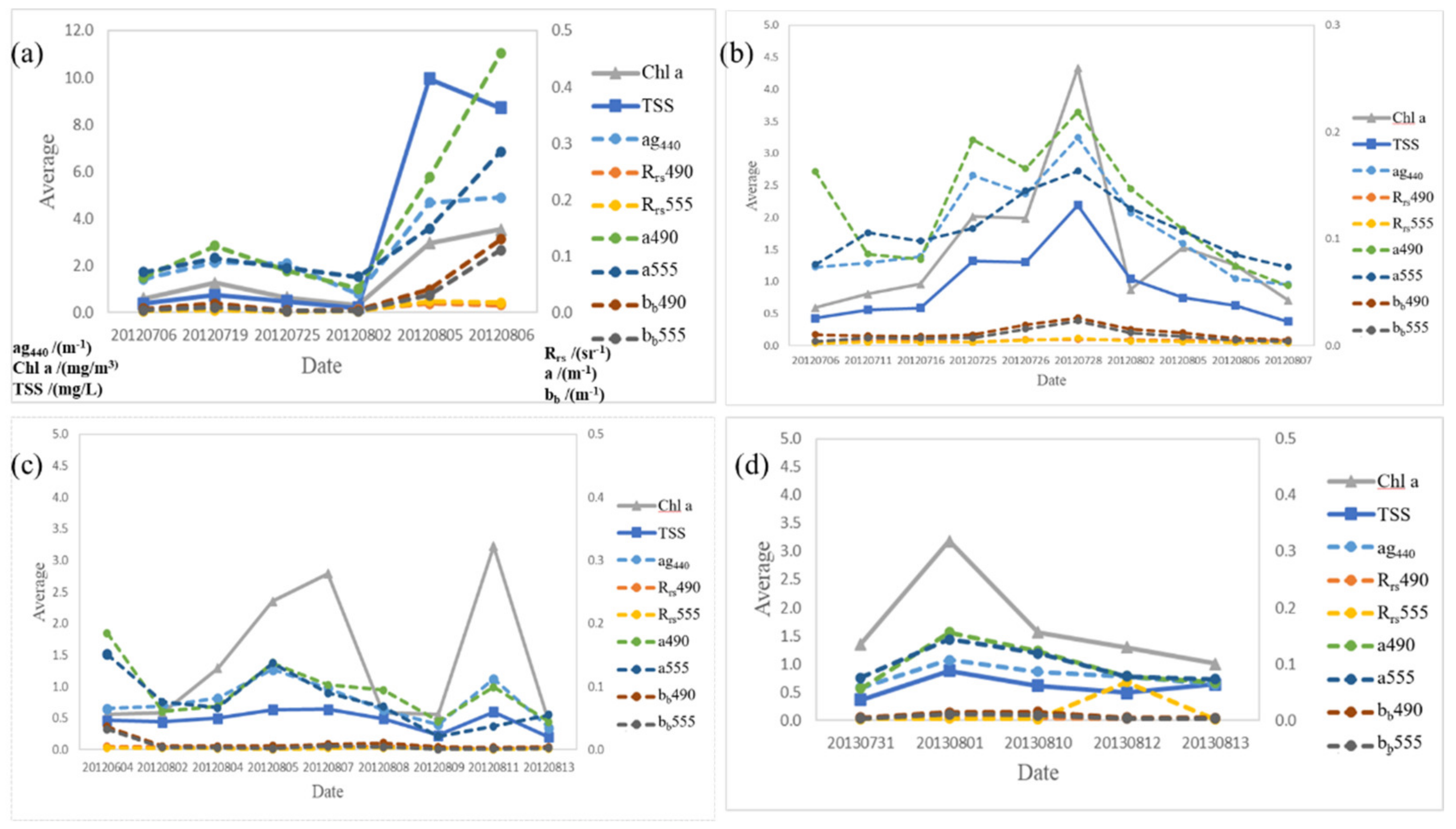
3.2. Comparison of Multiday Changes

We mark matched points and present the changes in Figure 7. The curves of different colors in Figure 7a are the trajectories of different drifting buoys, and the dots of different colors along the tracks show different values of ag440 measured at different sites. Similarly, Figure 7b shows the concentrations of Chl a and TSS with different colors, respectively. Buoy No. 2 lingered near the east coast of the Chinese mainland during its lifetime; meanwhile, Buoy No. 3 moved across the YS. The latter was located off the west coast of the Korean Peninsula from 2 August to 13 August. Buoys No. 3 and No. 7 were relatively far out to the sea, and the remaining buoys were closer to the coast. Among them, Buoy No. 1 was located near the coast on 5 and 6 August 2012, so its mean concentration of TSS was particularly high.
Figure 8 displays every buoy’s multiday-averaged variation. We can see that ag440, a, and bb were stable over a relatively long period. The event with high concentration of Chl a occurred following the movement of Buoy No. 2 in the summer of 2012. High Chl a lasted at least five days, increased from July 25 and started to decrease on 2 August 2012. Its peak reached 4.3 mg L−1. Meanwhile, its TSS appeared to be high. Being affected by both high Chl a and TSS, the measured optical absorption and backscattering coefficients at 490- and 555-nm bands both appeared high. The high Chl a event was also observed by Buoy No. 3. The first peak reached 2.8 mg L−1; and after a short falling down, it had another peak from 4 August to 13 August 2012. Following the movement of the water parcel, the high concentration of TSS was observed by Buoy No. 1. From 5 August 2012, Buoy No. 1 moved closely along the coast of China. Buoy No. 7 was far away from the other buoys, but the variations of parameters in the water parcel are similar to those in the other water parcels. Chlorophyll is also the parameter with the largest range of changes. These optical anomalies were diversely related to the specific biological and environmental conditions occurring in the study area.

3.3. GOCI Data Screening

In one-hour interval, the minimum movement tracked by the drifting buoy was 0.42 m s−1. According to the spatial resolution of GOCI imagery, the moving distance per hour of water parcel is about two pixels for buoys No. 1 and No. 5. For the other four drifters in 2012, the span of one-hour interval was three pixels or more, as shown in Table 5. Comparison to the Lagrangian observations, Eulerian observation includes the inertial oscillations caused by the tide.
In this study, the screening window is mainly determined by the movement speed of the water parcel followed by buoys. The restrictive matching condition produces different matching sets between drifter data and GOCI data. In addition, the choice of processing window size can affect the difference between the two time series. Therefore, different processing window sizes, such as 1 × 1, 3 × 3, and 5 × 5 pixels, were selected to obtain GOCI-derived products, and differences between the average values of the two time series were compared. When using window size 1 × 1, the matching pairs were reduced to 131 sites and the matching days were less than 23 days due to cloud cover in GOCI imagery.
The daily averaged difference is calculated as an average difference between the two series’ daily averages, and the daily-averaged difference divided by the daily average of Series-fixed is called daily mean relative difference. Table 6 shows that in the three window selection schemes, the larger the window is, the smaller the daily average difference between the two sets of sequences is; so the difference between the two series processed by 5 × 5 window is the smallest. In addition, the daily mean relative difference processed by the 5 × 5 window was within 9%, and the difference of TSS with the biggest change under various conditions reached 8.5%. The results show that under the 1 × 1 window, relatively small amount of data were obtained, and the relative percentage error was the largest.
The selection of processing window size should avoid overlap as much as possible in data processing. Taking all of the above factors into consideration, GOCI-derived data were computed by averaging 3×3 pixels surrounding the in situ measurement location, which gave us as many matching pairs as possible and as large difference as possible between the two time series.

4. Discussion

4.1. Impacts of Seasonality and Daytime on GOCI Data Processing

The negative impact from the sensor-solar geometry should be considered in the algorithms. As a geostationary satellite, the main uncertainty in the GOCI remote sensing reflectance for assessing diurnal variability of biogeochemical processes is the effect of solar zenith angle (SZA) between noon and twilight. During the processing of GOCI data, we examined the effect of SZA in the retrieval of remote sensing reflectance and derived products. In our case study, the operation of drifters lasted from June to August. The lifetimes of drifters covered the summer time. For this study region, the range of SZA during the acquisition time varied between 0° and 70° (Figure 9), more than half being less than 30°, and that for the sensor (viewing) zenith angle varied from approximately 45° to 54°; both criteria did not exclude any pixels.
Fairly uniform fields are seen in summer, with a very narrow range of variability for each product, indicating that the in-water properties are fairly stable during summer regardless of the SZA [51]. Only small effects from SZA appeared at the beginning and end of the day, presumably due to reduced sunlight. However, the effect of SZA is very minimal, and no obvious trend is observed. No trend was observed during different seasons and different times of the day, when the GOCI data versus SZA were analyzed [52]. Summer seems to yield the most ideal data for evaluating GOCI in this study area because of the very small variability for all the derived-products used.

4.2. Variation in Spatial Transition

Using the 40-m isobath to divide the near-shore and central regions of the YS/ECS, we calculated the mean, maximum and minimum values of optical properties of Series-moving and Series-fixed. The ranges near the shore were obviously greater than those in the central region. Figure 7 suggests that the water-mass movement in the YS basin was complex, and most of the water mass moved from shallow to deep water area. The value of ag440 offshore was higher than that in the central region. The changes in the blue box and green box in Figure 7a are more obvious. Combining the information in Table 7 with that in Figure 7, the variance of bio-optical properties of the offshore water was larger than that measured by the open-sea buoys, especially for the variance in Series-fixed. This means the bio-properties offshore changed more often with higher concentrations than their counterparts in the central region of the YS/ECS. As the diluted water enters the ocean with large amounts of sediment, phytoplankton, etc., it collides and merges with ocean water. In contrast, the central region of the YS/ECS shows a stable environment.
Study [48] suggested that the remotely sensed CDOM can be used as a passive tracer for freshwater input. The distribution of CDOM concentration is closely related to the distribution and characteristics of water mass. There are two sources of CDOM in the ocean: the land-based input of surface runoff and groundwater, and the marine source dominated by phytoplankton production and microbial degradation. The content of CDOM in fresh water is relatively high, and the mixing of fresh water and sea water will affect the distributions of ag440 and Chl a. In the areas close to the shore, the mixing of estuarine diluted water and sea water plays an important role. In the low-value area of the open sea, fresh water has less influence; CDOM mainly comes from plankton production. Combined with Figure 7 and Figure 8, we can see that the diurnal and multiday variation trends of CDOM absorption were almost consistent with those of Chl a. When Chl a concentration was abnormally high, ag440 would be relatively high. Combined with the location information in Figure 7, the relationship between CDOM and Chl a was closer in the central YS/ECS. We can further show the relationship between ag440 and plankton field production in the open sea. Here, the variation of concentration may be caused by alternation of water-mass movement and tidal changes.
The YOC algorithms proposed by Siswanto et al., 2011 [19] does not perform well in all cases. The absolute percent difference (APD) may be high at a range of 10−1 for CDOM. Future investigation will be carried out to improve the model and build regional algorithms.

4.3. Difference in Spatiotemporal Transition

The primary conclusion of this paper is that the in-water constituents within the water parcel change temporally and spatially over short or long periods of time. Specifically, any diurnal to spatial variability in the water parcel measurable by GOCI will be different. Here, statistical analyses on diurnal and two-day series were performed in order to distinguish these differences.
Figure 10 shows both daily and multiday trends of ag440, Chl a, and TSS based on data from buoys No. 2 and No. 3. TSS was affected mostly by tidal waves and tides in unstable offshore environment. The average of TSS concentration in the offshore waters around Buoy No. 2 was mostly above 0.5 mg L−1, and its maximum concentration reached 2.2 mg L−1 with the range of 1.8 mg L−1. The Chl a range was between 0.5 and 2.0 mg L−1, and the anomalies of high concentration emerged on 28 July. The average of TSS around Buoy No. 3 was about 0.5 mg L−1, which appeared relatively stable. The average of Chl a concentration in the offshore waters of the Korean Peninsula was from 0.5 to 3.0 mg L−1. The multiday change of time series indicate that these two water parcels were conspicuously different in terms of bio-optical properties. The change of chlorophyll per day might be heavily affected by the change in light intensity. In addition, the changes of various parameters in multidays might be heavily affected by the changes in location. Even when the daily variation ranges of parameters were large, the variation ranges of various parameters in the multidays were not large.
Considering the influence of time and space, we believe that the distance of water-parcel movement is relatively short in a day/8 hours, and the variation of parameters in the water parcel during this period can be assumed to be only or mainly affected by time, while the variation of parameters obtained from multiple days at noon can be assumed to be mainly influenced by space. Out of the matching days within the entire period investigated, there are only nine two-day series with valid values for all the bands. The value at 12:30 Beijing time was chosen as a reference because at this time of the day the value should be affected less by lower SZA than at early and late periods of the day. Therefore, the relative difference in the day/multiday with respect to the value at 12:30 was calculated. As shown in Figure 11, the relative difference in multiday is larger than that in the day, namely, the bio-optical properties of the water changed more during multiple days. The minimal difference in time of ag440 was 0.36%, while the minimal difference in space was 1.84%. In these two days, the differences impacted by time were within 20%, while the differences impacted by space were over 20% mostly, especially for Chl a. The GOCI-derived Chl a data at the location of Buoy No. 3 on 7 August 2012 were relatively large throughout the whole day, especially from 10:30 to 11:30. So, Group 6 showed a particularity that the relative variance in time exceeded that of the relative variance in space.

5. Conclusions

In this study, we developed a novel approach to observe diurnal variation of bio-optical properties in the moving surface water parcel, which tracks the movement of surface currents using drifting buoys, and combines its spatiotemporally matched bio-optical properties with the retrieval from the GOCI. This study was motivated by the need for an observational tool that complements studies of moving water parcel, and it lays a good foundation for further application.
The case study using the proposed method shows differences between the diurnal variation of time series with water-parcel movement and that of the traditional fixed-location time series. Although both time series had the same value at the same location from the beginning, the subsequent measurements became different. The average hourly relative differences of the two time series in the YS/ECS during the summers of 2012 and 2013 were up to 15.7% and 16.3% for Chl a and TSS, respectively. Furthermore, we show that ag440 in the moving water parcel was more stable than that at a fixed location. It is suitable to use a passive tracer for following a water mass.
The daily and multiday changes of Chl a and TSS are relatively complex, and the differences between the two time series are comparatively large. Further analysis showed that in the YS/ECS region, diurnal variation was spatially different. The range of offshore TSS was up to 9.76 mg L−1, which was higher than that of 0.74 mg L−1 in the central YS/ECS. The ranges of Chl a and ag440 offshore were higher than those in the central sea, namely, the diurnal variation of ocean color observations was more obvious in the nearshore water parcel.
We believe the novel approach can provide a new perspective for studying surface moving water parcel, which has relied on limited in situ measurements and numerical simulations, regardless of the limitations in the present study. The new approach will not only reduce the cost but also evaluate the moving water parcel, which should play an important role in observing diurnal variability of bio-optical properties in the moving surface water parcel.

Author Contributions

Conceptualization, J.C. and Y.X.; methodology, J.C. and Y.X.; software, Y.X.; data analysis, J.C., Y.X. and F.Q.; investigation, J.C and Y.X.; resources, W.G. and Z.C.; writing Y.X. and J.C.; supervision, J.C.; project administration, J.C.; funding acquisition, J.C. All authors have read and agreed to the submitted version of the manuscript.

Funding

This research was funded by the National Key Research and Development Program of China (Grant No. 2016YFC1400903), NSFC-Zhejiang Joint Fund for the Integration of Industrialization and Informatization (Grant No. U1609202), Key Special Project for Introduced Talents Team of Southern Marine Science and Engineering Guangdong Laboratory (Guangzhou) (GML2019ZD0602), and National Natural Science Foundation of China (Grant Nos. 42076216, 41376184, and 40976109).

Institutional Review Board Statement

Not applicable.

Informed Consent Statement

Not applicable.

Data Availability Statement

The authors thank the Korea Ocean Satellite Center (download URL: http://kosc.kiost.ac/, accessed on 19 June 2020) for providing GOCI data.

Conflicts of Interest

The authors declare no conflict of interest.

References

  1. Stramska, M.; Dickey, T.D. Variability of bio-optical properties of the upper ocean associated with diel cycles in phytoplankton population. J. Geophys. Res. Space Phys. 1992, 97, 17873–17887. [Google Scholar] [CrossRef]
  2. Loisel, H.; Vantrepotte, V.; Norkvist, K.; Mériaux, X.; Kheireddine, M.; Ras, J.; Pujo-Pay, M.; Combet, Y.; Leblanc, K.; Mauriac, R.; et al. Characterization of the bio-optical anomaly and diurnal variability of the particulate matter, as seen from the scattering and backscattering coefficients, in ultra-oligotrophic eddies of the Mediterranean Sea. Biogeosci. Discuss. 2011, 8, 7859–7919. [Google Scholar] [CrossRef] [Green Version]
  3. Gould, J.R.W.; Anderson, S.; Lewis, M.D.; Miller, W.D.; Shulman, I.; Smith, G.B.; Smith, T.A.; Wang, D.W.; Wijesekera, H.W. Assessing the impact of tides and atmospheric fronts on submesoscale physical and bio-optical distributions near a coastal convergence zone. Remote Sens. 2020, 12, 553. [Google Scholar] [CrossRef] [Green Version]
  4. Curran, K.; Hill, P.; Milligan, T.; Mikkelsen, O.; Law, B.; de Madron, X.D.; Bourrin, F. Settling velocity, effective density, and mass composition of suspended sediment in a coastal bottom boundary layer, Gulf of Lions, France. Cont. Shelf Res. 2007, 27, 1408–1421. [Google Scholar] [CrossRef]
  5. Hao, Y.; Cui, T.; Singh, V.P.; Zhang, J.; Yu, R.; Zhao, W. Diurnal variation of light absorption in the yellow river estuary. Remote Sens. 2018, 10, 542. [Google Scholar] [CrossRef] [Green Version]
  6. Song, K.; Li, L.; Li, S.; Tedesco, L.; Hall, B.; Li, L. Hyperspectral remote sensing of total Phosphorus (TP) in three central Indiana water supply reservoirs. Water Air Soil Pollut. 2011, 223, 1481–1502. [Google Scholar] [CrossRef]
  7. Le, C.; Hu, C.; Cannizzaro, J.; English, D.; Muller-Karger, F.; Lee, Z. Evaluation of chlorophyll-a remote sensing algorithms for an optically complex estuary. Remote Sens. Environ. 2013, 129, 75–89. [Google Scholar] [CrossRef]
  8. Huang, C.; Zou, J.; Li, Y.; Yang, H.; Shi, K.; Li, J.; Wang, Y.; Chena, X.; Zheng, F. Assessment of NIR-red algorithms for observation of chlorophyll-a in highly turbid inland waters in China. ISPRS J. Photogramm. Remote Sens. 2014, 93, 29–39. [Google Scholar] [CrossRef]
  9. Qi, L.; Hu, C.; Barnes, B.B.; Lee, Z. VIIRS captures phytoplankton vertical migration in the NE Gulf of Mexico. Harmful Algae 2017, 66, 40–46. [Google Scholar] [CrossRef]
  10. Arnone, R.; Vandermuelen, R.; Soto, I.; Ladner, S.; Ondrusek, M.; Yang, H. Diurnal changes in ocean color sensed in satellite imagery. J. Appl. Remote Sens. 2017, 11, 032406. [Google Scholar] [CrossRef] [Green Version]
  11. Amin, R.; Lewis, M.D.; Lawson, A.; Gould, R.W., Jr.; Martinolich, P.; Li, R.-R.; Ladner, S.; Gallegos, S. Comparative analysis of GOCI ocean color products. Sensors 2015, 15, 25703–25715. [Google Scholar] [CrossRef] [PubMed] [Green Version]
  12. Moon, J.-E.; Park, Y.-J.; Ryu, J.-H.; Choi, J.-K.; Ahn, J.-H.; Min, J.-E.; Son, Y.-B.; Lee, S.-J.; Han, H.-J.; Ahn, Y.-H. Initial validation of GOCI water products against in situ data collected around Korean peninsula for 2010–2011. Ocean Sci. J. 2012, 47, 261–277. [Google Scholar] [CrossRef]
  13. Min, J.-E.; Choi, J.-K.; Yang, H.; Lee, S.; Ryu, J.-H. Monitoring changes in suspended sediment concentration on the southwestern coast of Korea. J. Coast. Res. 2014, 70, 133–138. [Google Scholar] [CrossRef]
  14. Kim, W.; Moon, J.-E.; Park, Y.-J.; Ishizaka, J. Evaluation of chlorophyll retrievals from Geostationary Ocean Color Imager (GOCI) for the North-East Asian region. Remote Sens. Environ. 2016, 184, 482–495. [Google Scholar] [CrossRef]
  15. Zhang, M.; Tang, J.; Dong, Q.; Song, Q.; Ding, J. Retrieval of total suspended matter concentration in the Yellow and East China Seas from MODIS imagery. Remote Sens. Environ. 2010, 114, 392–403. [Google Scholar] [CrossRef]
  16. Doxaran, D.; Lamquin, N.; Park, Y.-J.; Mazeran, C.; Ryu, J.-H.; Wang, M.; Poteau, A. Retrieval of the seawater reflectance for suspended solids monitoring in the East China Sea using MODIS, MERIS and GOCI satellite data. Remote Sens. Environ. 2014, 146, 36–48. [Google Scholar] [CrossRef]
  17. Lou, X.; Hu, C. Diurnal changes of a harmful algal bloom in the East China Sea: Observations from GOCI. Remote Sens. Environ. 2014, 140, 562–572. [Google Scholar] [CrossRef]
  18. Wang, M.; Ahn, J.-H.; Jiang, L.; Shi, W.; Son, S.; Park, Y.-J.; Ryu, J.-H. Ocean color products from the Korean Geostationary Ocean Color Imager (GOCI). Opt. Express 2013, 21, 3835–3849. [Google Scholar] [CrossRef]
  19. Siswanto, E.; Tang, J.; Yamaguchi, H.; Ahn, Y.-H.; Ishizaka, J.; Yoo, S.; Kim, S.-W.; Kiyomoto, Y.; Yamada, K.; Chiang, C.; et al. Empirical ocean-color algorithms to retrieve chlorophyll-a, total suspended matter, and colored dissolved organic matter absorption coefficient in the Yellow and East China Seas. J. Oceanogr. 2011, 67, 627–650. [Google Scholar] [CrossRef]
  20. Yoon, J.-E.; Lim, J.-H.; Son, S.; Youn, S.-H.; Oh, H.-J.; Hwang, J.-D.; Kwon, J.-I.; Kim, S.-S.; Kim, I.-N. Assessment of satellite-based chlorophyll-a algorithms in eutrophic Korean coastal waters: Jinhae Bay case study. Front. Mar. Sci. 2019, 6, 359. [Google Scholar] [CrossRef]
  21. Li, H.; He, X.; Ding, J.; Hu, Z.; Cui, W.; Li, S.; Zhang, L. Validation of the remote sensing products retrieved by geostationary ocean color imager in Liaodong Bay in spring. Acta Opt. Sin. 2016, 36, 401002. [Google Scholar] [CrossRef]
  22. Son, Y.-T.; Park, J.-H.; Nam, S. Summertime episodic chlorophyll a blooms near the east coast of the Korean Peninsula. Biogeosciences 2018, 15, 5237–5247. [Google Scholar] [CrossRef] [Green Version]
  23. He, X.; Bai, Y.; Pan, D.; Huang, N.; Dong, X.; Chen, J.; Chen, C.-T.A.; Cui, Q. Using geostationary satellite ocean color data to map the diurnal dynamics of suspended particulate matter in coastal waters. Remote Sens. Environ. 2013, 133, 225–239. [Google Scholar] [CrossRef]
  24. Choi, J.-K.; Park, Y.J.; Lee, B.R.; Eom, J.; Moon, J.-E.; Ryu, J.-H. Application of the Geostationary Ocean Color Imager (GOCI) to mapping the temporal dynamics of coastal water turbidity. Remote Sens. Environ. 2014, 146, 24–35. [Google Scholar] [CrossRef]
  25. Noh, J.H.; Kim, W.; Son, S.H.; Ahn, J.-H.; Park, Y.-J. Remote quantification of Cochlodinium polykrikoides blooms occurring in the East Sea using geostationary ocean color imager (GOCI). Harmful Algae 2018, 73, 129–137. [Google Scholar] [CrossRef] [PubMed]
  26. Liu, X.; Wang, M. Analysis of ocean diurnal variations from the Korean Geostationary Ocean Color Imager measurements using the DINEOF method. Estuar. Coast. Shelf Sci. 2016, 180, 230–241. [Google Scholar] [CrossRef]
  27. Jiang, L.; Wang, M. Diurnal currents in the bohai sea derived from the Korean Geostationary Ocean Color Imager. IEEE Trans. Geosci. Remote Sens. 2016, 55, 1437–1450. [Google Scholar] [CrossRef]
  28. Lumpkin, R.; Özgökmen, T.; Centurioni, L. Advances in the application of surface drifters. Annu. Rev. Mar. Sci. 2017, 9, 59–81. [Google Scholar] [CrossRef] [Green Version]
  29. Chen, J.; Cao, Z.; Shen, Y.; Chen, J. Improving surface current estimation from Geostationary Ocean Color Imager using tidal ellipse and angular limitation. J. Geophys. Res. Oceans 2019, 124, 4322–4333. [Google Scholar] [CrossRef]
  30. Park, J.-E.; Park, K.-A.; Ullman, D.S.; Cornillon, P.C.; Park, Y.-J. Observation of diurnal variations in mesoscale eddy sea-surface currents using GOCI data. Remote. Sens. Lett. 2016, 7, 1131–1140. [Google Scholar] [CrossRef] [Green Version]
  31. Choi, J.; Park, Y.; Kim, W.; Kim, Y.H. Characterization of submesoscale turbulence in the east/Japan sea using Geostationary Ocean Color Satellite Images. Geophys. Res. Lett. 2019, 46, 8214–8223. [Google Scholar] [CrossRef]
  32. Paduan, J.D.; Washburn, L. High-Frequency radar observations of ocean surface currents. Annu. Rev. Mar. Sci. 2013, 5, 115–136. [Google Scholar] [CrossRef] [PubMed] [Green Version]
  33. Abbott, M.R.; Brink, K.H.; Booth, C.R.; Blasco, D.; Swenson, M.S.; Davis, C.O.; Codispoti, L.A. Scales of variability of bio-optical properties as observed from near-surface drifters. J. Geophys. Res. Space Phys. 1995, 100, 13345. [Google Scholar] [CrossRef] [Green Version]
  34. Davis, R.E. Drifter observations of coastal surface currents during CODE: The statistical and dynamical views. J. Geophys. Res. Space Phys. 1985, 90, 4756–4772. [Google Scholar] [CrossRef]
  35. Poulain, P.; Gerin, R. Assessment of the water-following capabilities of CODE drifters based on direct relative flow measurements. J. Atmos. Ocean. Technol. 2019, 36, 621–633. [Google Scholar] [CrossRef]
  36. Centurioni, L.; Oceanography, S.I.O.; Hormann, V.; Chao, Y.; Reverdin, G.; Font, J.; Lee, D.-K. Sea surface salinity observations with lagrangian drifters in the tropical North Atlantic during SPURS: Circulation, fluxes, and comparisons with remotely sensed salinity from aquarius. Oceanography 2015, 28, 96–105. [Google Scholar] [CrossRef] [Green Version]
  37. Turnbull, I.D.; Torbati, R.Z.; Taylor, R.S. Relative influences of the metocean forcings on the drifting ice pack and estimation of internal ice stress gradients in the L abrador S ea. J. Geophys. Res. Oceans 2017, 122, 5970–5997. [Google Scholar] [CrossRef]
  38. Yu, F.; Li, J.; Zhao, Y.; Li, Q.; Chen, G. Calibration of backward-in-time model using drifting buoys in the East China Sea. Oceanology 2017, 59, 238–247. [Google Scholar] [CrossRef]
  39. Ryu, J.-H.; Han, H.-J.; Cho, S.; Park, Y.-J.; Ahn, Y.-H. Overview of geostationary ocean color imager (GOCI) and GOCI data processing system (GDPS). Ocean Sci. J. 2012, 47, 223–233. [Google Scholar] [CrossRef]
  40. Santer, R.; Schmechtig, C. Adjacency effects on water surfaces: Primary scattering approximation and sensitivity study. Appl. Opt. 2000, 39, 361–375. [Google Scholar] [CrossRef]
  41. Feng, L.; Hu, C. Cloud adjacency effects on top-of-atmosphere radiance and ocean color data products: A statistical assessment. Remote Sens. Environ. 2016, 174, 301–313. [Google Scholar] [CrossRef]
  42. Bailey, S.W.; Werdell, P.J. A multi-sensor approach for the on-orbit validation of ocean color satellite data products. Remote Sens. Environ. 2006, 102, 12–23. [Google Scholar] [CrossRef]
  43. Chen, C.-T.A. Chemical and physical fronts in the Bohai, Yellow and East China seas. J. Mar. Syst. 2009, 78, 394–410. [Google Scholar] [CrossRef]
  44. Wang, J.; Yu, Z.; Wei, Q.; Yang, F.; Dong, M.; Li, D.; Gao, Z.; Yao, Q. Intra- and inter-seasonal variations in the hydrological characteristics and nutrient conditions in the southwestern Yellow Sea during spring to summer. Mar. Pollut. Bull. 2020, 156, 111139. [Google Scholar] [CrossRef] [PubMed]
  45. Peng, D.; Yang, Q.; Yang, H.-J.; Liu, H.; Zhu, Y.; Mu, Y. Analysis on the relationship between fisheries economic growth and marine environmental pollution in China’s coastal regions. Sci. Total. Environ. 2020, 713, 136641. [Google Scholar] [CrossRef] [PubMed]
  46. Xu, Y.; Sui, J.; Ma, L.; Li, X.; Wang, H.; Zhang, B. Temporal variation of macrobenthic community zonation over nearly 60 years and the effects of latitude and depth in the southern Yellow Sea and East China Sea. Sci. Total. Environ. 2020, 739, 139760. [Google Scholar] [CrossRef] [PubMed]
  47. Liu, Z.; Gan, J.; Hu, J.; Wu, H.; Cai, Z.; Deng, Y. Progress on circulation dynamics in the East China Sea and southern Yellow Sea: Origination, pathways, and destinations of shelf currents. Prog. Oceanogr. 2021, 193, 102553. [Google Scholar] [CrossRef]
  48. Ichikawa, H.; Beardsley, R.C. The Current System in the Yellow and East China Seas. J. Oceanogr. 2002, 58, 77–92. [Google Scholar] [CrossRef]
  49. Egbert, G.D.; Erofeeva, S.Y. Efficient inverse modeling of barotropic ocean tides. J. Atmos. Ocean. Technol. 2002, 19, 183–204. [Google Scholar] [CrossRef] [Green Version]
  50. Choi, J.K.; Hyun Yang, H.J.H.; Ryu, J.H.; Park, Y.J. Quantitative estimation of the suspended sediment movements in the coastal region using GOCI. J. Coast. Res. 2013, 65, 1367–1372. [Google Scholar] [CrossRef]
  51. Ferrari, G.; Dowell, M. CDOM Absorption characteristics with relation to fluorescence and salinity in coastal areas of the southern Baltic Sea. Estuar. Coast. Shelf Sci. 1998, 47, 91–105. [Google Scholar] [CrossRef]
  52. Concha, J.; Mannino, A.; Franz, B.; Kim, W. Uncertainties in the Geostationary Ocean Color Imager (GOCI) remote sensing reflectance for assessing diurnal variability of biogeochemical processes. Remote Sens. 2019, 11, 295. [Google Scholar] [CrossRef] [Green Version]
Figure 1. Diagram illustrating the proposed method. In the workflow of data processing, the trajectory of a drifter buoy is calculated and matched with GOCI data first. Then, the bio-optical properties obtained from matched pixel of GOCI products, including Chl a, ag440, and TSS, are added to expand the measurements of the buoy data that contain the longitude and latitude information as well as sampling time.
Remotesensing 13 02115 g001
Figure 2. A drifting buoy at work.
Remotesensing 13 02115 g002
Figure 3. A trajectory map showing drifting buoys used in this study. Lines with different colors represent the tracks of the seven drifting buoys. Buoys No. 1–No. 6 collected data from June to August in 2012, while Buoy No. 7 operated in 2013. “No. 1–No. 7” are used to mark the initial releasing locations of the buoys. Bathymetry is indicated by contours from light to dark blue for the range of 10 to 80 m. The dark lines with arrowhead show the main ocean currents in the area [47]. The Zhe-min costal current is close to the coastline. There is the Yellow Sea Cold Water Mass between the Yellow Sea Costal Current (YSCC) and the Korean Peninsula Coastal Current.
Remotesensing 13 02115 g003
Figure 4. Tidal currents in the study area, based on OSU data. The red, magenta, and blue arrows indicate the changing directions of three tidal current field in continuous time. (a) The red arrows represent the flow field at 10:30 Beijing time; (b) the magenta arrows represent the flow field at 11:30; and (c) the blue arrows represent the flow field at 12:30.
Remotesensing 13 02115 g004
Figure 5. Two types of time series constructed using daily images of GOCI. The sampling location of series-fixed was fixed (the yellow diamond). The sampling location of Series-moving changed (the red dot), which corresponded to the moving water parcel. The first sampling location at 8:30 Beijing time is the same for both time series.
Remotesensing 13 02115 g005
Figure 6. Comparison of four typical groups of diurnal time series. The dashed lines represent the fixed-location monitoring results using the traditional Eulerian method, and the solid lines represent the results of the proposed method. (a) Time series near Buoy No. 2 on 16 July 2012; (b) time series near Buoy No. 2 on 5 August 2012; (c) time series near Buoy No. 3 on 13 August 2012; and (d) Time series near Buoy No. 7 on 10 August 2013.
Remotesensing 13 02115 g006
Figure 7. Drifting buoy tracks and ocean color constituent concentrations measured at each site. The upper left image in (a) depicts the properties’ values of each matched point on the map, with different range of ag440 and colors. The remaining panels in (b) show enlarged matched areas for Chl a and TSS, respectively.
Remotesensing 13 02115 g007
Figure 8. Daily-averaged bio-optical properties evolved in the drifting buoy’s lifetime: Buoy No. 1 (a), No. 2 (b), No. 3 (c), and No. 7 (d). The parameter range of the solid line is shown by the left y-axis, while that of the dashed line, by the right y-axis.
Remotesensing 13 02115 g008
Figure 9. Solar zenith angle (a) and sensor zenith angle (b) for the GOCI mission. Only data that passed the exclusion criteria are used. The data are separated by the time of the day.
Remotesensing 13 02115 g009
Figure 10. Multiday variation of buoys. No. 2 (a) and No. 3 (b). It shows the distribution characteristics and overall trends of multiday ag440, Chl a, and TSS.
Remotesensing 13 02115 g010
Figure 11. Relative differences in space/time transition. Relative differences are displayed in different colors for three parameters of Chl a, ag440, and TSS. The hollow and solid symbols represent the relative differences of each parameter impacted by space mainly or time mainly.
Remotesensing 13 02115 g011
Table 1. Detail of drifting buoy lifecycle.
Drifting Buoy DurationTotal DaysScope of
Longitude
Scope of
Latitude
Total Sites
No. 15 June 2012–10 August 201266120°–122°E33°–37°N1460
No. 23 June 2012–20 August 201278120°–124°E34°–37°N1974
No. 33 June 2012–20 August 201278121°–125°E34°–39°N1765
No. 44 June 2012–4 July 201231120°–122°E33°–36°N665
No. 53 June 2012–19 July 201246120°–122°E33°–37°N982
No. 63 June 2012–11 June 20128120°–121°E33°–35°N164
No. 730 June 2012–26 August 201328122°–127°E29°–34°N375
Table 2. Matched days and sites.
Drifting BuoyTotal DaysMatched DaysDaily Matchup Sites
No. 16664, 4, 6, 4, 4, 8
No. 278104, 8, 7, 6, 4, 7, 4, 5, 8, 7
No. 37894, 8, 8, 8, 5, 5, 5, 4, 7
No. 43114
No. 54624, 4
No. 6800
No. 72858, 7, 6, 5, 7
Table 3. Statistics of bio-optical properties on six matched days.
Drifting Buoy DateSeries ag440Chl aTSSRrs(490)Rrs(555)
No. 211 July 2012Movingmean0.0770.8040.5590.0050.003
variance18.9%16.2%17.4%20.0%12.9%
Fixedmean0.0770.8220.5550.0050.003
variance19.6%18.0%17.2%20.4%9.7%
25 July 2012Movingmean0.1592.0151.3220.0030.003
variance16.5%20.9%34.9%25.0%12.9%
Fixedmean0.1391.9390.9760.0020.002
variance19.4%28.0%28.3%83.3%72.7%
5 August 2012Movingmean0.0961.5290.7460.0050.004
variance4.5%17.6%4.4%5.7%2.7%
Fixedmean0.1151.8780.9520.0050.004
variance18.5%22.7%21.5%7.5%7.1%
No. 34 June 2012Movingmean0.0660.5670.4650.0050.003
variance6.7%10.9%9.2%4.0%3.5%
Fixedmean0.060.4570.4140.0050.003
variance13.1%16.3%16.3%15.2%11.5%
2 August 2012Movingmean0.0690.5880.4420.0040.003
variance18.6%37.0%22.2%14.0%16.0%
Fixedmean0.090.9260.6010.0040.003
variance22.0%56.9%23.6%37.8%32.0%
No. 71 August 2012Movingmean0.1073.1840.880.0050.004
variance39.7%76.8%45.8%40.2%39.0%
Fixedmean0.113.3410.9040.0050.004
variance42.1%89.4%47.9%42.2%40.0%
Table 4. The overall variation at all matched sites.
Series ag440Chl aTSSa(490)a(555)bb(490)bb(555)
Movingmean0.0871.3760.6490.1020.0940.0100.007
max0.2117.7022.3130.5390.3590.0540.039
min0.0260.1380.0620.0390.0070.0030.001
range0.1847.5642.2510.5000.3520.10510.038
Fixedmean0.0881.3380.6600.0980.0960.0100.007
max0.2029.1832.3000.6240.3510.0400.036
min0.0260.1190.1320.0380.0090.0040.001
range0.1769.0642.1670.5860.3410.0370.035
Table 5. List of average speed and moving speed.
Drifting BuoyNo. 1No. 2No. 3No. 4No. 5No. 7
Average speed (km h−1)0.801.241.881.891.181.45
Table 6. Differences under different window sizes.
Window size ag440Chl aTSS
1 × 1Difference0.0070.1420.079
Percentage8.8%11.0%12.2%
3 × 3Difference0.0060.1110.059
Percentage7.6%9.5%8.8%
5 × 5Difference0.0040.0790.049
Percentage4.8%6.6%8.5%
Table 7. Regional differences of variation.
Location Series ag440Chl aTSSa(490)a(555)bb(490)bb(555)
Central
region of the Yellow and East China Seas
Movingmean0.0801.3770.5540.0040.0060.0920.089
variance41.5%88.8%51.8%32.7%243.3%73.3%55.7%
Fixedmean0.0821.3110.5980.0880.0890.0080.006
variance37.8%82.5%51.2%78.4%50.5%63.8%70.0%
OffshoreMovingmean0.1161.6742.2380.1810.1400.0360.030
variance53.1%84.9%151.1%86.8%69.8%145.1%159.1%
Fixedmean0.1141.7092.1930.1620.1290.0290.024
variance51.8%85.0%154.5%82.0%66.3%148.0%166.6%
Publisher’s Note: MDPI stays neutral with regard to jurisdictional claims in published maps and institutional affiliations.

