
A New Faulty GNSS Measurement Detection and Exclusion Algorithm for Urban Vehicle Positioning


1
College of Civil Aviation, Nanjing University of Aeronautics and Astronautics, Nanjing 211106, China
2
State Key Laboratory of Air Traffic Management System and Technology, Nanjing 210007, China
3
Department of Civil and Environmental Engineering, Imperial College London, London SW7 2AZ, UK
*
Author to whom correspondence should be addressed.
Remote Sens. 2021, 13(11), 2117; https://0-doi-org.brum.beds.ac.uk/10.3390/rs13112117
Submission received: 19 April 2021
/
Revised: 14 May 2021
/
Accepted: 21 May 2021
/
Published: 28 May 2021
(This article belongs to the Special Issue Integrated Applications of Real-Time GNSS Precise Positioning Services)
Abstract
:The performance requirements for Global Navigation Satellite Systems (GNSS) are becoming more demanding as the range of mission-critical vehicular applications, including the Unmanned Aerial Vehicle (UAV) and ground vehicle-based applications, increases. However, the accuracy and reliability of GNSS in some environments, such as in urban areas, are often affected by non-line-of-sight (NLOS) signals and multipath effects. It is therefore essential to develop an effective fault detection scheme that can be applied to GNSS observations so as to ensure that the vehicle positioning can be calculated with a high accuracy. In this paper, we propose an online dataset based faulty GNSS measurement detection and exclusion algorithm for vehicle positioning that takes account of the NLOS/multipath affected scenarios. The proposed algorithm enables a real-time online dataset based fault detection and exclusion scheme, which makes it possible to detect multiple faults in different satellites simultaneously and accurately, thereby allowing real-time quality control of GNSS measurements in dynamic urban positioning applications. The algorithm was tested with simulated/artificial step errors in various scenarios in the measured pseudoranges from a dataset acquired from a UAV in an open area. Furthermore, a real-world test was also conducted with a ground-vehicle driving in a dense urban environment to validate the practical efficiency of the proposed algorithm. The UAV based simulation exhibits a fault detection rate of 100% for both single and multi-satellite fault scenarios, with the horizontal positioning accuracy improved to about 1 metre from tens of metres after fault detection and exclusion. The ground vehicle-based real test shows an overall improvement of 26.1% in 3D positioning accuracy in an urban area compared to the traditional least square method.
1. Introduction
Unmanned aerial vehicles (UAVs) and ground vehicles are emerging mobile platforms that can be beneficial to many mission-critical applications in smart cities. These include delivery, search and rescue missions, and civil security [1]. In order to support these mission-critical applications, the on-board navigation system, especially the Global Navigation Satellite System (GNSS), is essential for providing accurate and reliable Positioning Navigation and Timing (PNT) information. In practice, however, the accuracy and reliability of GNSS positioning is always affected by a variety issues in urban areas, especially in respect to pseudorange-based positioning. The increased positioning uncertainty that arises from a mixture of faulty signals is a result of the signal challenges posed by urban areas, mainly due to the NLOS/multipath effects from the surrounding environments (e.g., skylines, canyons, tunnels, etc., seen in Figure 1). In addition, malfunctions in the satellite clock, an incorrect modelling of orbits, the ionisation of satellite payload silicon material, and inter-channel bias could also contribute to the excessive positioning errors [2]. It is therefore very important to guarantee that the GNSS signals received from different satellites are correct and accurate, since these are related to GNSS positioning performance and integrity evaluation.
In order to deal with this issue, a satellite navigation integrity monitoring scheme is proposed within the receiver, i.e., a Receiver Autonomous Integrity Monitoring (RAIM) system. This seeks to detect significant measurement errors arising from satellite malfunctions, the propagation environment, and others, by the use of information including redundant measurements, the geometrical configuration of satellites relative to the users, and knowledge of nominal error behaviour [3].
In developing our proposed solution, we consulted the extensive existing literature on GNSS quality control methods for RAIM type systems. One commonly used technique, for example, is the signal weighting-based method [4]. The key idea of this method is to use one or multiple variables (e.g., C/N0 or elevation angle or their combination, etc.) of the observed pseudorange to obtain proportional weights and thus better-quality signals in the positioning calculation. Furthermore, a number of algorithms for NLOS/multipath classification and thereafter mitigation or exploitation have been developed in recent years for environments such as urban areas. These strategies mainly include signal processing, antenna design, and measurement-based modelling. Signal processing strategies distinguish the multipath and LOS signals based on the different characteristics of the correlation functions. The correlation aims to obtain an optimal approximation of the signal range [5,6], and some correlator-related and Delay-Locked Loop (DLL) technologies have been proposed for error mitigation, including narrow correlators, high-resolution correlators, strobe correlators, shaping correlators, and Multipath Estimating Delay Lock Loop (MEDLL), etc. [6,7]. Receiver signal processing techniques can help to separate out the components of a multipath contaminated signal, but they are useless if there is no direct LOS component. Antenna design strategies, meanwhile, include the use of antenna arrays, choke-ring antennas, and other types of antennas to mitigate the multipath effects and then improve the positioning performance [8,9]. Measurement-based strategies include integrating GNSS observables, measurements, and satellite and signal information with other information sources. For example, using the GNSS elevation angle, pseudorange rate, C/N0, Doppler, etc., with the data from external aids such as Inertial Measurement Units (IMU), map aiding, ray tracing, etc., to improve the positioning performance [10,11,12].
Fault Detection and Exclusion (FDE) algorithms are also widely used for RAIM, these include: (1) range and position comparison methods [13]; (2) least squares residuals methods (LSRM) [14]; (3) parity space methods [15]; and (4) maximum slope (MS) methods [16]. Various extensions have been further developed from these basic methods. For example, Brown applied an improved MS method, denoted as the slope-max-max method, by imposing a worst-case hypothetical two-failure requirement on RAIM to handle dual satellite failures [17]. Since the traditional RAIM algorithms are designed only for horizontal position monitoring, advanced RAIM (ARAIM) has emerged and therein the prospect of handling any number of simultaneous significant measurement errors, as well as vertical integrity monitoring [18]. Usually, FDE schemes entail both global and local tests, where the global test is used to check for the presence of any fault (for which a minimum of five satellites is required) and then the local test is used to identify the precise fault (for which six satellites are required). A common approach to performing the global test is to use a test statistic, based on the Normalised Sum of Squared Error (NSSE), checking whether or not this variable, multiplied by a variance factor and by the degrees of freedom (n-p), follows a centrally chi-squared distribution [19]. Basic FDE algorithms are able to detect and exclude one fault in all measures, whereas more advanced recursive consistency checking based methods are able to exclude multiple faults in the measures. Blanch et al. proposed a greedy search and an L1 norm minimisation combinatorial method for multiple fault detection and exclusion (FDE) with pseudorange errors above 20 m [20]. Similarly, Hsu et al. used greedy and exhaustive methods to improve the consistency checking process of the FDE [21]. These consistency check based FDE algorithms are only effective when at least six satellites can be observed, however. In addition, although optimisation algorithms are used for the subset search, the calculation efficiency is still a major issue with increased satellite numbers. Kaddour et al. proposed a multi-faults detection algorithm based on an observation projection on the information space [22]. The positioning estimation is then calculated by excluding the pseudorange measurement faults from the information filter process. In the designed Kalman Filter (KF) process, the state vector is based on the simple difference, with the satellite with the highest elevation angle being the reference at each epoch. In urban canyons, however, the rapid changes in reference satellites may lead to a reduced performance of the algorithm.
For the weighting and FDE-based methods for RAIM discussed above, the current signal weighting-based methods find it difficult to determine the weightings in urban areas. For example, satellites with a lower elevation angle along the street direction may suffer from less NLOS than satellites with higher elevation angles in the crossing street direction. The current FDE algorithms are also not robust enough in these kinds of situations. Some of the algorithms use the single fault assumption, which is not suitable for urban vehicle positioning because the environment changes rapidly and individual satellites can therefore be associated with faulty signals at one instant, and not at the next instant. This means that the fault associated with the current satellite may be gone in the next epoch but then it may reappear again with either the same or a new satellite in the next epoch. Thus, the single fault assumption is not realistic in urban areas.
In addition, most of the multiple fault detection algorithms require at least six satellites for the FDE, which is difficult to achieve in an urban context. Furthermore, the huge number of subsets in the consistency check reduce the calculation efficiency of these algorithms. This is a big issue in the context of fault detection for vehicle positioning since the detection of faults, and the consequent recalculation of the solution, needs to be completed fast enough so as not to exceed the necessary reaction time for the vehicles, especially for vehicle applications that involve live subjects.
In this context, this paper proposes a new faulty GNSS measurement detection and exclusion algorithm for the dynamic positioning of vehicles in urban environments. The proposed algorithm has a dual-dynamic online dataset generation scheme, which contains the latest features of the pseudoranges in the urban areas and is therefore able to achieve a high accuracy and fast fault detection and exclusion in dynamically changing environments. The proposed algorithm can be operated with only four satellites and is sensitive to small faults, which are suitable for urban areas where there is often poor access to satellites. The contributions are summarised below.
- 1.
- The development of a new faulty GNSS measurement detection and exclusion algorithm to achieve simultaneous multi-fault detection and exclusion, which is sensitive to small pseudorange faults and therefore could improve the accuracy and integrity of the urban positioning.
- 2.
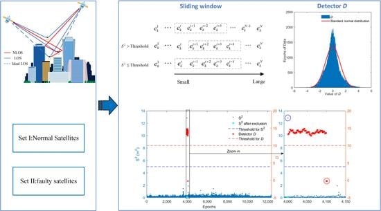
- The design of two dynamic online datasets (i.e., a real-time normal dataset and a “non-trusted” dataset) within the algorithm to ensure that the latest features of the fault pseudoranges in the changing environments are always available. In particular, a sliding window, based on the pseudorange KF innovations from satellites in the normal satellite’s dataset, is designed to check satellites maintaining normal data, while detector D, which is generated based on the difference between the predicted pseudorange and the observed pseudorange using data from satellites in the faulty satellite’s dataset, is designed for checking faulty satellites or those just coming into view.
- 3.
- A test and a validation of the efficiency of a proposed algorithm using simulations with simulated/artificial step errors in various scenarios on the measured pseudoranges from a dataset acquired from a UAV in an open area, and a real-world test with a ground-vehicle in a dense urban environment.
2. GNSS FDE Algorithm for Urban Positioning
2.1. System Framework
The flowchart for the proposed FDE-based positioning algorithm is presented in Figure 2. Before a mission is assigned, it is necessary to conduct an initialisation of the receiver using a Suggestion Range Consensus (S-RANCO) [23], in a relative open sky area, which could be satisfied frequently in urban areas. The purpose of the initialisation is to use this method aimed at multi-faults as the reference to create the initial datasets, using the measurements from these satellites with both “normal” and “fault” measurements, identified and labelled from the onboard GNSS receiver (as described in Section 2.2, algorithm initialisation).
The “normal” measurements are stored in the dataset named “Set I” and the “non-trustable” measurements are stored in the dataset named “Set II” (this initially contains only satellites with faulty measurements, but during the operation it will contain “new” satellites that did not exist at last epoch, which may or may not have faulty measurements), shown in Figure 3 as an example. During the operation, once a new observation (which means the satellite is observed at a specific epoch) is received, a judgement is carried out to check whether this satellite has already been tracked in Set I, in which case the observed information is added to Set I (contains tracked satellites), otherwise the observed measurements are added in Set II (contains faulty satellites and newly observed satellites). Although the sliding window and the detector are applied separately for fault detection, fault removal and recovery, Set I and Set II are then constantly updated according to the detection results at each epoch with satellites re-assigned between the sets by the proposed algorithm
In particular, the sliding window, whose size is changeable, is executed based on the KF innovations of the observed pseudoranges in Set I. The satellite with a faulty measurement at a specific epoch is determined by an evaluation of the variance of innovations within the adaptive window. The determination of the window should meet two requirements: (1) the final window should contain the maximum number of normal satellites observed, and (2) the variance of the innovations within the final window is less than the predetermined threshold (details described in Section 2.4).
Then, the satellites inside of the window are considered as normal satellites and kept in Set I, while those outside are flagged as faulty satellites and are moved to Set II.
The detector D, is created based on the difference in the observed pseudoranges of the satellites in Set II and the predicted pseudoranges, calculated based on the real-time position obtained from the positioning solutions of the satellites in Set I at the current epoch, and the measurement information of the satellites in Set II, to check whether these satellites (already in Set II or newly observed satellites in Set II) are normal or not (Section 2.5). The D results are then compared with the threshold T to determine whether the satellite is still presenting faulty data or recovering to normal, and the movement of the corresponding satellites between the sets will be carried out accordingly. Once the faulty satellite in Set II is excluded, the |D|, the absolute value of D, immediately drops below the threshold. If the |D| value remains below the threshold for two consecutive epochs, we will move the satellite back to Set I where it would be used at that epoch for the positioning calculation. The threshold determination for D is described in Section 2.5 as well.
The final positioning will be the output if the usable number of satellites in Set I (NSet I) is equal to or greater than four.
2.2. Algorithm Initialisation
As described above, our proposed process requires an initialization process in a relative open sky area using the S-RANCO based algorithm. The S-RANCO based algorithm is designed for multi-fault detection and exclusion, and the available measurements in open sky are less likely to have faults. Therefore, it is possible to detect the faulty measurements based on the test statistics resulting from the collected pseudoranges in relative open areas. Thus, the Initial Set I and II are represented as follows:
where Initial Set I contains the set of satellites returning normal data during the initialisation process, and to represent the ID of these satellites, from 1 to n. Meanwhile, Initial Set II contains the set of satellites returning faulty measurements, and to represent the ID of these satellites, from 1 to . All the historical measurements are included in the sets for the specific satellites, including the raw measurements of pseudorange, satellite position, etc.
2.3. Pseudorange Change Based Transition Model
Before a description of the fault detection and exclusion model, the transition model for the GNSS measurements needs to be designed. The pseudorange is one of the most important observations in GNSS, and the accuracy of the pseudorange contributes significantly to the accuracy of the positioning. In the case of the satellites returning faulty data, the associated NLOS, multipath and satellite clock errors are expressed in the form of pseudorange errors. The pseudorange measurement is merely the travel time scaled by the speed of light in a vacuum, and can be expressed as:
where is the geometric range between the user position and the satellite position; and reflect the delays related to the transmission of the signal through the ionosphere and troposphere, respectively; , and are the receiver clock error, satellite clock error and other modelled or unmodelled errors, respectively. According to Equation (3), in epochs and , the pseudorange measurement can be expressed through Equation (4) and Equation (5), respectively:
The satellite clock bias , tropospheric error , ionospheric error , and other measurement errors (e.g., ephemeris error), only change a little within a short time instant and hence can be neglected based on the time-differenced model [24]. Time-differenced pseudorange measurements can be expressed as follows, using Equation (4) and Equation (5):
where and are the changes in the pseudorange and the geometric range between two measurement epochs; is the variation of the receiver clock errors at two adjacent epochs. The remaining measurement error, which is not removed through calculating the time differences, is denoted with . These residual errors are considered to be negligible for the purposes of this process, however. in k epoch can be represented as:
where and are the geometric ranges between the receiver position and the satellite position at two epochs, and ; and are the satellite position vectors at two epochs; and are the receiver position vectors, and and are the unit vectors pointing to the satellite from the receiver position. We consider that is approximately equal to due to the remote distance between the satellite and the receiver. Therefore, when the two epochs are very close together in time, we can obtain:
where and are the changes in the geometric range of the satellite and the receiver between two epochs in an Earth Centred Earth Fixed (ECEF) coordinates frame.
According to Equation (6) and Equation (8), we can obtain:
If the acceleration of the vehicle (such as a UAV) is a in a specific direction, then the difference of the position change between two adjacent epochs is , where is the time interval. When is 0.1 s, taking m/s2as an example, the corresponding value is 0.1 m, which is small enough and can be neglected within the fault detection algorithm. It is to be noted that the proposed algorithm is for civil applications in urban areas; these vehicles (e.g., UAVs and ground vehicles) have low accelerations (e.g., less than 10 m/s2). Here, the movement of the vehicle can be considered as a continuously linear motion at a constant speed in a very short time (e.g., within 1 s). Similarly, the movement of the satellites can be considered as a linear motion at a constant speed in a very short time (e.g., within 1 s), because of their stable circular motion. Therefore, our algorithm is applicable for the sharp turn of a vehicle in urban areas since it can be considered as an accelerated motion.
It is to be noted that may change during the consecutive two epochs. Here, we have defined the changes of between epoch and as (in the unit of s). The hypothesis test is designed for two alternative transition models used in the Kalman filter, which will be described in Section 2.4.
For H0: the is 0, according to (9) and the described motion principles above. The transition model can be defined as:
and H1: the is not 0.
where Δε is the random noise.
2.4. Sliding Window Based Fault Detection for Set I
The fault detection for the pseudoranges in Set I is based on the well-known KF approach, which has been applied in many applications to obtain an optimal estimation accuracy with a low computation complexity [25]. With the transition models established in Section 2.3, the state vector (Equation (12)) and observation vector (Equation (13)) are designed based on Equations (10) and (11) and are as follows:
For H0:
and H1:
The state transition equation and measurement equations are in Equation (15) and Equation (16).
where,
is the state vector in the time epoch k.
is the state vector in the time epoch .
is the transition matrix, which is equal to the identity matrix.
is the process noise in the time epoch k−1 with the covariance matrix .
is the measurement at the time epoch k.
is the measurement noise in the time epoch k with the covariance matrix .
is the measurement mapping matrix, which equals to identity matrix.
The innovation sequence, , which is the difference between the observed value and the KF predicted value, is generated in order to detect the faults in the data from each satellite in Set I:
where, is the pseudorange change propagation from the time epoch to . follows a white Gaussian sequence in a long time period. Over short timeframes, however, its mean and standard deviation vary according to the velocity, the quality of the receiver, the elevation of the satellites, and the condition of the troposphere, ionosphere, etc. [26].
In the proposed algorithm, we first use the transition model of the KF to predict the pseudorange change of the observed satellites. In this prediction step, we assume the does not change initially, which means is 0. At the same time, we obtain the observed pseudorange change. With the difference between the observed pseudorange and the predicted pseudorange changes (i.e., the innovation ), we evaluate the results based on the proposed check algorithm, i.e., sliding window. Both the real faulty measurement of the satellite and result in the changes of the observed , and they have different characteristics for both cases. For example, the change of caused by NLOS is not equal for all satellites, because NLOS signals are received from different directions in urban areas, while the will cause an equal length to every satellite in the change of , further resulting in the almost equal . Therefore, we can use the variance of to determine the case at that epoch. If the is less than a specific determined threshold, we can consider that the changes of are caused by the receiver clock. Otherwise, we can consider that the changes of are caused by a real fault, such as NLOS. The can be expressed as follows:
Here, n is the number of satellites; is the KF innovation of each satellite at k epoch; is the mean of all the KF innovations detected at the k epoch, and is the variance. The distribution of the value is in Figure 4. When the value of is smaller than the threshold (under the confidence level of 99.9%) (Gatti, 1984), which is 5.11 and 23.53 for UAVs and ground vehicles in urban areas from a priori data, respectively, in this paper, we can consider that these measurements of satellites are not faulty. However, when non-zero and real faults occur simultaneously, the will become much bigger than the threshold too. If we consider all the satellites as faulty, the satellite availability will be degraded in a real-world situation. In order to solve this problem, assuming that N satellites are received by the receiver at epoch k, to find the satellite which includes both the non-zero and the real faults from those only containing non-zero , an adaptive sliding window is designed as follows.
- 1.
- Sort all of the (I = 1, 2 … N) of satellites in Set I at epoch k from the smallest (left) to the largest (right), shown in Figure 5.
- 2.
- Use a sliding window for the smallest four and then calculate the of the current window.
- 3.
- If the is above the threshold, we will discard the first in the window (flagged as the fault satellite) and move one step of the window to the right side with the window size unchanged. Then the new will be further checked with the threshold. This process will be stopped until all have been checked or is less than the threshold. For the former, we consider that there is no satellite that can be used to calculate the position of the receiver at this epoch, and all of the satellites at this epoch will be moved to Set II. For the latter, go to the next step.
- 4.
- If the is within the threshold, the satellites in the window can be used for positioning. Therefore, we consider them as satellites only containing non-zero . In order to improve the positioning performance, it is preferable to use as many satellites as possible. Then the window size (e.g., four) will be extended to the right side with one more , which means the next innovation will be included in the window. Then the of this new window will be checked with the threshold again. If the is still within the threshold, we will repeat the process of step 4. If the is greater than the threshold, as the newly added results in the big deviation of the , then all of the on the right side of this one will be flagged as faulty satellites. The process will be turned to step 5.
- 5.
- Finally, the satellites inside of the window will be considered as normal satellites and those outside of the window will be flagged as faulty satellites. The faulty satellites will then be put into Set II and the normal satellites will be put into Set I. The mean value of the innovations for all normal satellites, , can be regarded as the value of at this epoch. Once a non-zero is confirmed, we substitute for in for this epoch and the filtering process will be repeated. However, for the next epoch, the . in will still be set as zero initially for the filtering process until a non-zero is detected again.
2.5. Faulty Measurement Monitoring Algorithm for Set II
Because the vehicle is moving relatively fast in NLOS/multipath-affected urban environments, the visibility of the satellites changes frequently. This means that newly observed satellites may suffer from the effects of NLOS or multipath, while the satellites originally in Set II may return to normal. Detector D is therefore created for real-time fault status monitoring. Specifically, the satellites in Set I for a given epoch are used to calculate the position and the receiver clock error. We then combine them with the modelled ionospheric, tropospheric errors, the Klobuchar model and the Saastamoinen model, respectively, with parameters from the ephemeris data, and the positions and clock errors of the satellites in Set II to predict the pseudoranges of these satellites, respectively. The predicted pseudorange and the observed pseudorange are then compared. The pseudorange prediction equation is:
where, is the predicted pseudorange, and is the distance between the satellite position and the vehicle position calculated by the satellites in Set I. is the estimated receiver clock error. and are the ionospheric and tropospheric errors estimated by the models. By subtracting the observed pseudorange from the predicted pseudorange , we obtain:
Then we define the detector D for each faulty or newly observed satellite as follows:
where j is the satellite number; and are the a priori mean and standard deviations of . The |D| is then compared with the threshold T to determine whether the satellite still has a faulty measurement or has recovered to normal. The faulty satellites remain in Set II while the normal ones are moved to Set I.
The a priori data we used for each satellite in the simulation (open area) and real experiment (urban) are empirical models with 0 m mean and 0.7 m standard deviations, and 0 m mean and 4 m standard deviation normal distributions respectively. The a priori data are obtained from previous UAV tests and ground vehicle tests.
After the normalization in (21), the distribution of the detector D can be considered to follow a standard normal distribution. Figure 6 is an example of the distribution of the detector D from the real UAV flight test. In general, the detection threshold T is determined according to the principle [27]. However, in a real case, we can choose a larger value of T based on the requirement of the system positioning accuracy. However, the minimum value of T should be no less than the value. By using this strategy, some minor errors are inevitable in the pseudorange measurements. Nevertheless, it is not necessary to remove all errors completely, since where errors are small enough not to affect our positioning results, removing those satellites so as to rely on a smaller number of satellites with poor geometries for positioning would risk enlarging positioning errors. For this reason, it is critical to achieve a trade-off between the satellite number and the pseudorange quality in the determination of the threshold. Therefore, we set , which is much bigger than the value (i.e., 3).
3. Simulation of Faulty Measurements in the UAV Flight Test
The simulation of faulty measurements scenarios in the UAV flight data was to test the proposed fault detection and exclusion algorithm. The UAV flight test data was collected in Nantou City, Taiwan, with the flight route shown in Figure 7. The raw pseudorange measurements were collected from a dual-frequency GNSS receiver, Trimble BD 982, with a sampling rate of 10 Hz. The UAV used in the test was an AXH-E230 from AVIX Technology and was flown semi-automatic. It is equipped with intelligent autopilot system AJC and a smart power control module system to perform an autonomous intelligent navigation flight mission. The speed of the UAV was less than 10 m/s during the flight and the height was about 60 m AGL (with the ground elevation around 120 m). The reference trajectory used in the experiment was obtained from close range photogrammetry providing centimetre-level positioning accuracy using the on-board VLP-16 Velodyne Lidar. Four defined fault scenarios were added to the real trajectory: a single step error for Scenario 1 and multiple step errors for Scenarios 2, 3 and 4. The details for the four scenarios are described in Table 1.
In Scenario 1, we conducted one hundred durations of the experiment for each value of the range error added in the observed satellites. For every randomly chosen satellite at each time, pseudorange errors of between 10 and 50 metres were added in a specific time duration of 10 s. The reason for not considering errors less than 10 m is that these would not contribute significant positioning errors in the pseudorange-based positioning calculation. The proposed algorithm can be used for satellite quality control if less than five satellites are observed at one epoch. Nevertheless, for the purposes of this experiment, we only chose epochs with more than six satellites observed so as to ensure sufficient satellites for calculating the positioning solution.
Figure 8 is an example of the fault detection results for satellite SV10. For the step errors added in SV10 during epoch 4000–4100, the sliding window could be triggered to detect the fault. This would move SV10 to Set II and then the detector D would be applied to monitor the ongoing quality of SV10 in Set II. Once the faulty satellite SV10 is excluded, the value of D will immediately drop below the threshold. Afterwards, we moved the SV10 back to Set I, in which the pseudorange measurements were used for the positioning calculation at that epoch. It is indicated in the results in Table 2 that the proposed algorithm could achieve a 100% correct detection rate for pseudorange errors above 10 m. It is also indicated that the proposed algorithm is superior to the S-RANCO based algorithm in the correction detection rates, which are 66% for a 20 m pseudorange error and 0% for a 10 m pseudorange error.
In Scenario 2, we again conducted one hundred iterations of the experiment for each defined fault case. For both of the randomly chosen two satellites, 10 m, 20 m, 30 m, 40 m or 50 m pseudorange errors were added in specific time epoch durations, i.e., the errors could start from any epoch and last for 10 s during the test. Because in this scenario there were two satellites with errors in a given epoch, we chose those time epochs where more than six satellites were observable. The proposed algorithm is based on every single satellite and is therefore very effective in detecting simultaneous errors in two satellites. Here we have defined a valid successful detection as occurring only when the faults in each of the two satellites are detected. From Table 3, it is shown that the proposed algorithm achieved a 100% correct detection rate in the case of two satellites with simultaneous errors, while the counterparts of the S-RANCO based algorithm are 0%, 9%, 52%, 98% and 100% corresponding to the increasing pseudorange errors. The detailed comparison of this is summarised in Table 4. The proposed algorithm also has the advantage of being able to detect faults even when only four satellites are available, and it is also very sensitive to small faults, neither of which is the case with the S-RANCO based algorithm. The only disadvantage of the proposed algorithm is that it requires historical information or an initialisation process.
In Scenario 3, in order to test the performance of the proposed algorithm under the condition where various multipath/NLOS errors mixed with non-zero , the 20 m and 50 m errors were added to both of the randomly chosen two satellites, while 100 m was added to all the available satellites at a specific epoch. We conducted one hundred iterations of this experiment for defined fault cases at epochs where more than six satellites were observable. The valid successful detection was the same as Scenario 2. In Table 5, it is presented that the proposed algorithm achieved 100% correct detection for the case of two satellites with simultaneous errors and a non-zero . Table 6 shows the details of how our sliding window worked as an experiment. The value of is very small when the window does not contain the with both errors and a non-zero , but it would increase a hundredfold when the window includes an of a faulty satellite. Therefore, the proposed algorithm is able to detect the satellite with only a non-zero and the satellite with both a fault and a non-zero .
Scenario 4 was designed to evaluate the proposed algorithm under the condition where the normal satellites were less than 4. Errors of −60 m, −40 m, 20 m, 30 m and 60 m were added to five satellites, respectively, and a 100 m was added in all satellites received at this epoch. Table 7 depicts an example of the windowing process. It is clear that the value of for each of the four satellites is above the threshold, and thus cannot be used for positioning. In this scenario, the proposed algorithm can still be effective, but the positioning cannot be calculated due to insufficient normal satellites at the epoch.
In order to further investigate the effectiveness of the proposed algorithm for the final positioning results, we calculated the positioning solutions for the epochs with faulty satellites and compared them with the results of different fault detection and exclusion methods, which are the S-RANCO and proposed algorithms. The Root Mean Square Error (RMSE) was used to evaluate the positioning results with these FDE algorithms applied one hundred times. Table 8 shows the positioning results with and without these algorithms in Scenario 1. It is indicated that the 3D position accuracy RMSE was 4.47 m with the proposed algorithm applied, while without the FDE, it was 13.79 m, 24.15 m, 34.15 m, 45.00 m and 55.44 m for the single satellite with faults of 10 m, 20 m, 30 m, 40 m and 50 m. The results of the S-RANCO based method were not as good as the results of the proposed method. The details are shown in Table 8. The positioning results with and without FDE algorithms in Scenario 2 are shown in Table 9. It is indicated that the 3D positioning accuracy was 10.79 m after the proposed FDE was applied, while it varied from 27.94 m to 126.52 m with the various magnitude of errors added in the simulation in Scenario 2. The results of the remaining method are shown in Table 9. Table 10 indicates the 3D positioning accuracy with FDE was 2.70 m in Scenario 3, exhibiting an improvement of 93.6% over the positioning results without FDE.
4. Ground Vehicle Test in Deep Urban Environments
The real field test with a ground vehicle was used to further validate the proposed algorithm in the simultaneous multi-fault environments, i.e., the deep urban environment. A ground vehicle with an onboard dual-frequency GNSS receiver, Pwrpak E1, with a sampling rate of 1 Hz, was conducted to collect the raw GNSS data for around half an hour in Kaohsiung City, Taiwan. Although the dual-frequency GNSS receiver was used for the data collection, only the single frequency (i.e., L1) measurement data were used for the positioning. The reference trajectory of the vehicle position used in the experiment was post-processed with the commercial software NovAtel Inertial Explorer from the onboard real-time kinematic (RTK) GNSS and a navigation-grade IMU (RQH) integration. The positioning performance using the proposed FDE algorithm on the pseudorange measurements from the collected raw GNSS data was then evaluated with the reference trajectory.
The test trajectory is illustrated in Figure 9 and the vehicle velocity ranges between 0 and 30 m/s. The positioning accuracy performance using the proposed algorithm is shown in Figure 10. The numerical analysis of the accuracy in terms of RMSE is shown in Table 11. As we will never know the “real” fault of the received measurements, the final positioning results were analyzed to evaluate the performance of proposed FDE algorithm.
The proposed algorithm demonstrates the effectiveness of the positioning accuracy improvement in urban areas. From Table 11, it can be seen that the improvement in the positioning accuracy from the FDE based GNSS positioning algorithm is 30.47%, 7.72% and 27.24% in East, North and Up directions when compared with that from traditional single point positioning. The horizontal and 3D positioning accuracy has been improved to 8.3 m and 18.0 m from 10.6 m and 24.3 m, respectively, with improvements of about 21% and 26% using the proposed FDE algorithm. In contrast, the S-RANCO based algorithm only shows limited capability in improving the performance of GNSS positioning results, with only 1.9% and 5.3% improvements in horizontal and 3D, respectively. What is worse, the positioning error enlarges by 9.7% in a North direction. It is indicated from Figure 10 that for the epochs around 300 s, the proposed algorithm can even provide an improvement of up to about 80% in both horizontal and height positioning results, while the S-RANCO based algorithm cannot acquire such achievement. The overall improvement of about 26% is because the NLOS does not exist at each epoch. Our algorithm cannot improve the positioning accuracy of the epochs without NLOS, therefore the improvement of partial epochs would be reduced by using the whole epochs to calculate the positioning accuracy.
5. Conclusions
We have proposed a new faulty GNSS measurement detection and exclusion algorithm for vehicle positioning. The simulation test with various satellite pseudorange errors demonstrates the effectiveness of the proposed algorithm, with a fault detection rate of 100% for the scenarios of single and multi-satellite measurement faults. It is demonstrated that four satellites are enough for the proposed algorithm to be used for fault detection, which is very useful in urban navigation. The horizontal positioning RMSE has been improved to 1.2 m, 0.96 m, and 2.03 m with the proposed algorithm in Scenarios 1, 2 and 3, respectively. The corresponding 3D RMSE is 4.47 m, 10.79 m, and 2.70 m. This compares to accuracies in the tens of metres (horizontal) and more than 100 metres (3D) based on the pseudorange errors introduced in the satellites. The results from a real deep urban test with a ground vehicle show that the proposed algorithm provideds a horizontal and 3D positioning RMSE of 8.1 m and 17.5 m using only the single frequency pseudorange measurements. The proposed algorithm has both horizontal and 3D improvements of about 21% and 26% compared to the traditional single point positioning method.
The main issue with the proposed algorithm is that an initialisation is required. In addition, as the historical information from the initialisation is required to generate the test statistics, loss of lock during the test will affect the performance of the algorithm. A task for future research, therefore, is to design a more robust initialisation scheme that integrates with the IMU for operations in urban environments.
Author Contributions
Conceptualization, Q.C. and R.S.; Data curation, J.W.; Formal analysis, Q.C.; Methodology, Q.C. and R.S.; Software, J.W.; Supervision, P.C., Y.M. and W.Y.O.; Writing—original draft, Q.C.; Writing—review & editing, R.S. and W.Y.O. All authors have read and agreed to the published version of the manuscript.
Funding
This work was supported in part by the sponsorship of the National Natural Science Foundation of China under Grant 41974033, in part by the Fundamental Research Funds for the Central Universities under Grant KFJJ20200705, in part by Zhe Jiang Key laboratory of General Aviation Operation technology (General Aviation Institute of Zhejiang JianDe) under Grant JDGA2020-11, in part by States Key Laboratory of Air Traffic Management System and Technology under Grant SKLATM201904, in part by the Six Talent Peak Project of Jiangsu Province under Grant KTHY-014, and in part by Horizon 2020 EU-China Aviation Technology Cooperation Project.
Acknowledgments
Thanks for Kai-Wei Chiang form National Cheng Kung University to provide data.
Conflicts of Interest
The authors declare no conflict of interest.
References
- Colomina, I.; Molina, P. Unmanned aerial systems for photogrammetry and remote sensing: A review. ISPRS J. Photogramm. Remote Sens. 2014, 92, 79–97. [Google Scholar] [CrossRef] [Green Version]
- Bhatti, U.I.; Ochieng, W.Y. Failure modes and models for integrated GPS/INS systems. J. Navig. 2007, 60, 327–348. [Google Scholar] [CrossRef]
- Bhatti, U.I. Improved Integrity Algorithms for the Integrated GPS/INS Systems in the Presence of Slowly Growing Errors. Ph.D. Thesis, Imperial College London, London, UK, 2007. [Google Scholar]
- Wieser, A.; Brunner, F.K. An extended weight model for GPS phase observations. Earth Planets Space 2000, 52, 777–782. [Google Scholar] [CrossRef] [Green Version]
- Heinrichs, G.; Lemke, N.; Neubauer, A.; Kronberger, R.; Schmid, A.; Rohmer, G.; Förster, F.; Avila-Rodriguez, J.A.; Pany, T.; Eissfeller, B.; et al. Galileo/GPS Receiver Architecture for High Sensitivity Acquisition. In Proceedings of the International Symposium on Signals, Systems, and Electronics (ISSSE’04), Linz, Austria, 10–13 August 2004. [Google Scholar]
- Blanch, J.; Walter, T.; Lee, Y.; Pervan, B.; Rippl, M.; Spletter, A. Advanced RAIM user algorithm description: Integrity support message processing, fault detection, exclusion, and protection level calculation. In Proceedings of the 25th International Technical Meeting of the Satellite Division of The Institute of Navigation, (ION GNSS+ 2012), Savannah, GA, USA, 22–25 September 2012; pp. 2828–2849. [Google Scholar]
- Nee, R.D.J.V. The Multipath Estimating Delay Lock Loop. In Proceedings of the ISSTA IEEE Second International Symposium on Spread Spectrum Techniques and Applications, Yokohama, Japan, 29 November–2 December 1992. [Google Scholar]
- Thornberg, D.B.; Thornberg, D.S.; Dibenedetto, M.F.; Braasch, M.S.; Graas, F.V.; Bartone, C. LAAS Integrated Multipath-Limiting Antenna. Navigation 2003, 50, 117–130. [Google Scholar] [CrossRef]
- Groves, P.; Jiang, Z.; Rudi, M.; Strode, P. A Portfolio Approach to NLOS and Multipath Mitigation in Dense Urban Areas. In Proceedings of the 26th International Technical Meeting of the Satellite Division of The Institute of Navigation (ION GNSS+ 2013), Nashville, TN, USA, 16–20 September 2013; pp. 3231–3247. [Google Scholar]
- Soloviev, A.; Graas, F.V. Utilizing multipath reflections in deeply integrated GPS/INS architecture for navigation in urban environments. In Proceedings of the 2008 IEEE/ION Position, Location and Navigation Symposium, Monterey, CA, USA, 5–8 May 2008; pp. 383–393. [Google Scholar]
- Meguro, J.I.; Murata, T.; Takiguchi, J.I.; Amano, Y.; Hashizume, T. GPS multipath mitigation for urban area using omnidirectional infrared camera. IEEE Trans. Intell. Transp. Syst. 2009, 10, 22–30. [Google Scholar] [CrossRef]
- Groves, P. Shadow Matching: A New GNSS Positioning Technique for Urban Canyons. J. Navig. 2011, 64, 417–430. [Google Scholar] [CrossRef]
- Lee, Y.C. Analysis of Range and Position Comparison Methods as a Means to Provide GPS Integrity in the User Receiver. In Proceedings of the 42nd Annual Meeting of The Institute of Navigation, Seattle, WA, USA, 24–26 June 2004. [Google Scholar]
- Parkinson, B.W.; Axelrad, P. Autonomous GPS Integrity Monitoring Using the Pseudorange Residual. Navigation 1988, 35, 255–274. [Google Scholar] [CrossRef]
- Sturza, M.A. Navigation System Integrity Monitoring Using Redundant Measurements. Navigation 1988, 35, 483–501. [Google Scholar] [CrossRef]
- Brown, R.G.; McBurney, P.W. Self-Contained GPS Integrity Check Using Maximum Solution Separation. Navigation 1988, 35, 41–53. [Google Scholar] [CrossRef]
- Brown, R.G. Solution of the Two-Failure GPS RAIM Problem under Worst-Case Bias Conditions: Parity Space Approach. Navigation 1997, 44, 425–431. [Google Scholar] [CrossRef]
- Rippl, M.; Spletter, A.; Günther, C. Parametric Performance Study of Advanced Receiver Autonomous Integrity Monitoring (ARAIM) for Combined GNSS Constellations. In Proceedings of the 2011 International Technical Meeting of the Institute of Navigation, San Diego, CA, USA, 24–26 January 2011. [Google Scholar]
- Kuusniemi, H.; Lachapelle, G. GNSS signal reliability testing in urban and indoor environments. In Proceedings of the 2004 National Technical Meeting of the Institute of Navigation, San Diego, CA, USA, 1–15 August 2004. [Google Scholar]
- Blanch, J.; Walter, T.; Enge, P. Efficient multiple fault exclusion with a large number of pseudorange measurements. In Proceedings of the 2015 International Technical Meeting of the Institute of Navigation, Dana Point, CA, USA, 26–28 January 2015; pp. 696–701. [Google Scholar]
- Hsu, L.T.; Tokura, H.; Kubo, N.; Gu, Y.; Kamijo, S. Multiple faulty gnss measurement exclusion based on consistency check in urban canyons. IEEE Sens. J. 2017, 99, 1909–1917. [Google Scholar] [CrossRef]
- Kaddour, M.A.; Najjar, M.E.B.E.; Naja, Z.; Moubayed, N.; Tmazirte, N.D.A. Fault detection and exclusion for GNSS measurements using observations projection on information space. In Proceedings of the Fifth International Conference on Digital Information & Communication Technology & Its Applications, Beirut, Lebanon, 29 April–1 May 2015. [Google Scholar]
- Schroth, G.; Ene, A.; Blanch, J.; Walter, T.; Enge, P. Failure Detection and Exclusion via Range Consensus. In Proceedings of the European Navigation Conference 2008, DLR, Toulouse, France, 25 April 2008. [Google Scholar]
- Soon, B.K.H.; Scheding, S.; Lee, H.K.; Lee, H.K.; Durrant-Whyte, H. An approach to aid INS using time-differenced GPS carrier phase (TDCP) measurements. Gps Solut. 2008, 12, 261–271. [Google Scholar] [CrossRef]
- Welch, G. Kalman Filter; Siggraph Tutorial: Los Angeles, CA, USA, 2001. [Google Scholar]
- Maybeck, P.S. Stochastic Models, Estimation, and Control; AcAcademic Press: Cambridge, MA, USA, 1982; Volume 1. [Google Scholar]
- Gatti, P.L. Probability Theory and Mathematical Statistics for Engineers; Pergamon Press: Oxford, UK, 1984. [Google Scholar]
Figure 1.
Illustration of LOS and NLOS.

Figure 2.
System framework.

Figure 3.
Normal satellite set (blue) and non-trustable satellite set (red).
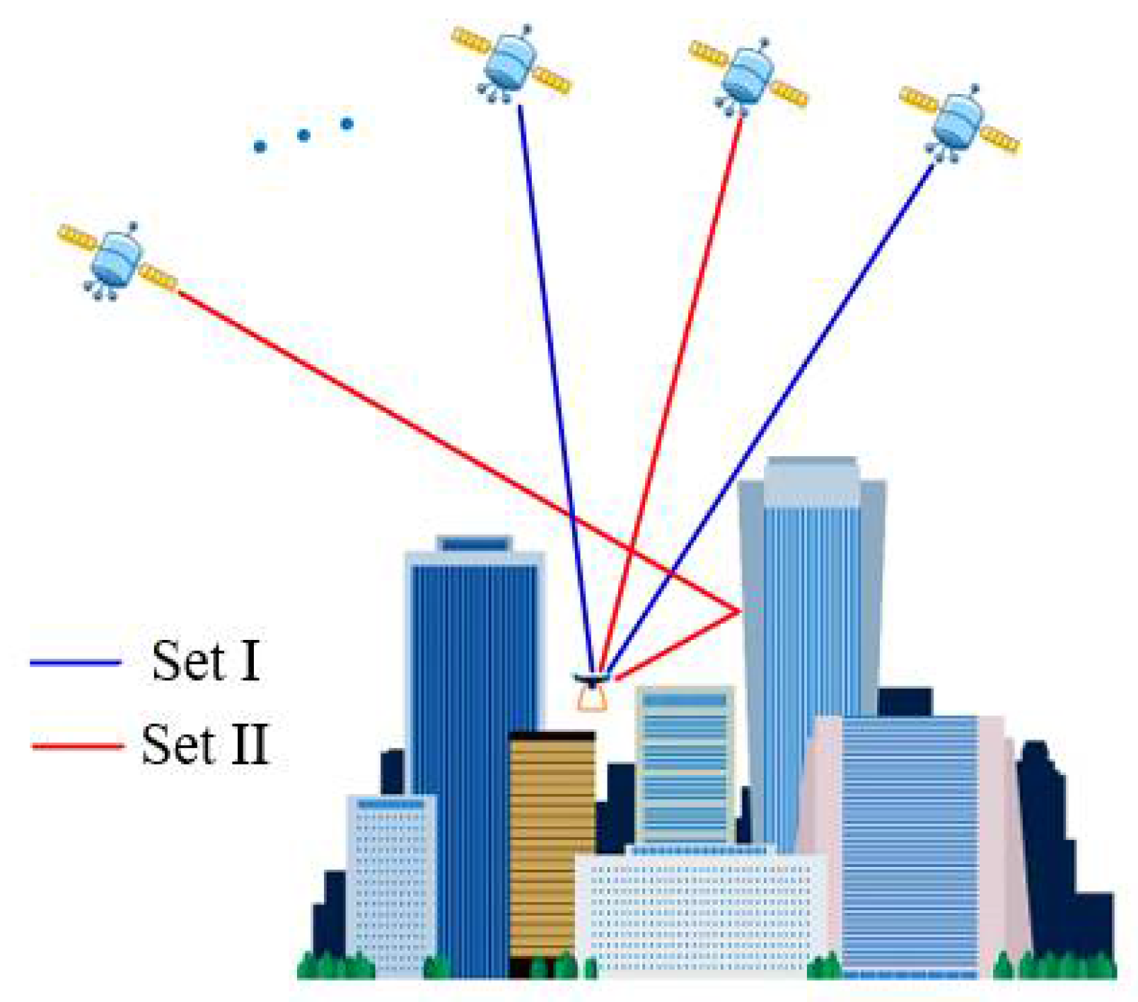
Figure 4.
The distribution of .
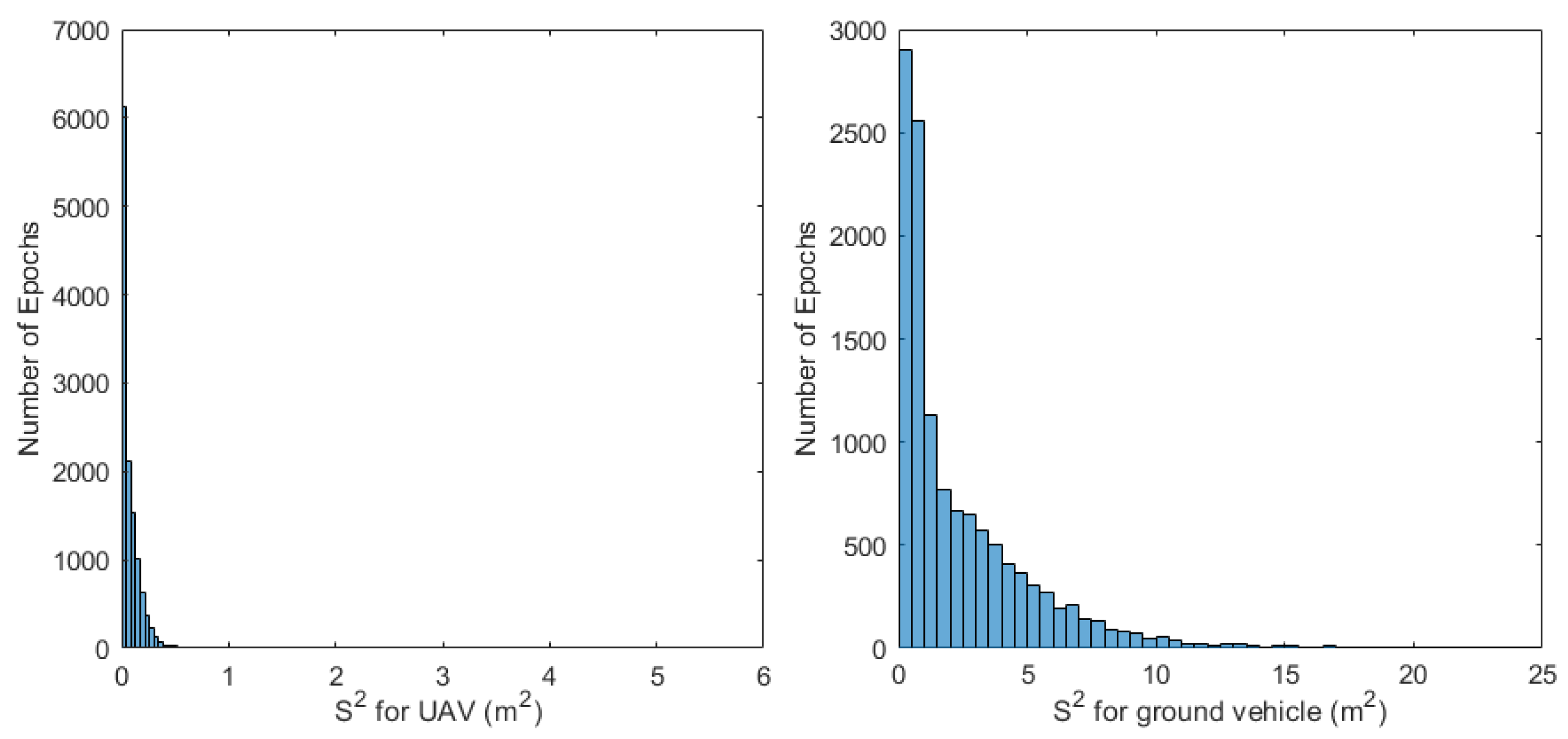
Figure 5.
Windowing process for fault detection based on Set I.
Figure 6.
Distribution of the value of D for the UAV test.

Figure 7.
UAV flight trajectory.

Figure 8.
An example of the fault detection results for satellite SV10.

Figure 9.
Urban test trajectory.

Figure 10.
Positioning errors of the traditional method and the proposed FDE based method.

Table 1.
The defined scenarios.
| Scenarios | Fault Satellites Numbers | Duration Time (s) | Number of Test | Error Sources |
|---|---|---|---|---|
| 1 | Single-fault | 10 | 100 | 10~50 m range error added to one satellite with an interval of 10 m |
| 2 | dual-fault | 10 | 100 | 10~50 m range error added to two satellites with an interval of 10 m respectively |
| 3 | dual-fault | 0.1 | 100 | 20 m and 50 m errors added to two satellites respectively and 100 m added to all satellites at one epoch |
| 4 | multi-fault | 0.1 | 1 | −60 m, −40 m, 20 m, 30 m and 60 m errors added to 5 satellites respectively and 100 m added to all satellites at one epoch |
Table 2.
Comparison of algorithms performance with various values of error sources in Scenario 1.
| Error Source (m) | Number of Test | Correct Detection Rate (Proposed Method) | Correct Detection Rate (S-RANCO Based) |
|---|---|---|---|
| 10 | 100 | 100% | 0% |
| 20 | 100 | 100% | 66% |
| 30 | 100 | 100% | 100% |
| 40 | 100 | 100% | 100% |
| 50 | 100 | 100% | 100% |
Table 3.
Comparison of algorithms performance with various values of error sources in Scenario 2.
| Error Source (m) | Number of Test | Correct Detection Rate (Proposed Method) | Correct Detection Rate (S-RANCO Based) |
|---|---|---|---|
| 10 | 100 | 100% | 0% |
| 20 | 100 | 100% | 9% |
| 30 | 100 | 100% | 52% |
| 40 | 100 | 100% | 98% |
| 50 | 100 | 100% | 100% |
Table 4.
Comparison between the proposed method and S-RANCO based method.
| Proposed Method | S-RANCO Based Method | |
|---|---|---|
| Historical information required | Yes | No |
| Simultaneous multiple faults detection | Yes | Yes |
| The minimum number of SVs required for fault detection | ≥4 | ≥5 |
| The minimum number of SVs required for fault exclusion | ≥4 | ≥6 |
| Sensitive to small faults | Yes | No |
Table 5.
Comparison of algorithms performance with various values of error sources in Scenario 3.
| Error Source (m) | Number of Test | Correct Detection Rate (Proposed Method) | Correct Detection Rate (S-RANCO based) |
|---|---|---|---|
| 20 and 50 | 100 | 100% | 100% |
Table 6.
An example of windowing results in Scenario 3.
| Satellite ID | 20 | 25 | 15 | 32 | 10 | 24 | 12 | 21 |
| (m) | 100 | 100 | 100 | 100 | 100 | 100 | 100 | 100 |
| Step error (m) | 0 | 0 | 0 | 0 | 0 | 0 | 20 | 50 |
| (after sorting) | 99.43 | 99.46 | 99.63 | 99.85 | 99.92 | 101.11 | 119.38 | 149.35 |
| 0.04 | / | / | / | / | ||||
| 0.05 | / | / | / | |||||
| 0.39 | / | / | ||||||
| 54.55 | / | |||||||
| 319.01 | ||||||||
Table 7.
An example of windowing results in Scenario 4.
| Satellite ID | 12 | 15 | 32 | 10 | 24 | 20 | 21 | 25 |
| (m) | 150 | 150 | 150 | 150 | 150 | 150 | 150 | 150 |
| Step error (m) | −60 | −40 | 0 | 0 | 0 | 20 | 30 | 60 |
| (after sorting) | 89.38 | 109.63 | 149.85 | 149.92 | 151.11 | 169.43 | 179.35 | 209.46 |
| 914.28 | / | / | / | / | ||||
| / | 413.66 | / | / | / | ||||
| / | / | 91.87 | / | / | ||||
| / | / | / | 206.65 | / | ||||
| / | / | / | / | 595.31 | ||||
Table 8.
The RMSE (m) of positioning results for Scenario 1.
| Single Step Error (m) | 10 | 20 | 30 | 40 | 50 | |
|---|---|---|---|---|---|---|
| East | Without FDE | 2.31 | 4.21 | 6.10 | 8.00 | 9.90 |
| S-RANCO | 2.31 | 1.60 | 0.61 | 0.61 | 0.61 | |
| Proposed method | 0.61 | 0.61 | 0.61 | 0.61 | 0.61 | |
| North | Without FDE | 1.19 | 3.48 | 5.78 | 8.08 | 10.38 |
| S-RANCO | 1.19 | 1.81 | 1.04 | 1.04 | 1.04 | |
| Proposed method | 1.04 | 1.04 | 1.04 | 1.04 | 1.04 | |
| Up | Without FDE | 13.54 | 23.53 | 33.53 | 43.54 | 53.55 |
| S-RANCO | 13.54 | 11.96 | 4.31 | 4.31 | 4.31 | |
| Proposed method | 4.31 | 4.31 | 4.31 | 4.31 | 4.31 | |
| Horizontal | Without FDE | 2.60 | 5.46 | 8.40 | 11.37 | 14.35 |
| S-RANCO | 2.60 | 2.42 | 1.20 | 1.20 | 1.20 | |
| Proposed method | 1.20 | 1.20 | 1.20 | 1.20 | 1.20 | |
| 3D | Without FDE | 13.79 | 24.15 | 34.56 | 45.00 | 55.44 |
| S-RANCO | 13.79 | 12.20 | 4.47 | 4.47 | 4.47 | |
| Proposed method | 4.47 | 4.47 | 4.47 | 4.47 | 4.47 | |
Table 9.
The RMSE (m) of positioning results for Scenario 2.
| Double Step Error (m) | 10 | 20 | 30 | 40 | 50 | |
|---|---|---|---|---|---|---|
| East | Without FDE | 1.52 | 2.60 | 3.69 | 4.78 | 5.88 |
| S-RANCO | 1.52 | 2.06 | 2.08 | 0.79 | 0.77 | |
| Proposed method | 0.77 | 0.77 | 0.77 | 0.77 | 0.77 | |
| North | Without FDE | 3.79 | 8.71 | 13.63 | 18.55 | 23.47 |
| S-RANCO | 3.79 | 8.53 | 11.11 | 1.65 | 0.58 | |
| Proposed method | 0.58 | 0.58 | 0.58 | 0.58 | 0.58 | |
| Up | Without FDE | 27.64 | 51.76 | 75.90 | 100.04 | 124.19 |
| S-RANCO | 27.64 | 50.40 | 55.85 | 13.71 | 10.74 | |
| Proposed method | 10.74 | 10.74 | 10.74 | 10.74 | 10.74 | |
| Horizontal | Without FDE | 4.09 | 9.09 | 14.12 | 19.15 | 24.19 |
| S-RANCO | 4.09 | 8.78 | 11.30 | 1.83 | 0.96 | |
| Proposed method | 0.96 | 0.96 | 0.96 | 0.96 | 0.96 | |
| 3D | Without FDE | 27.94 | 52.56 | 77.20 | 101.86 | 126.52 |
| S-RANCO | 27.94 | 51.16 | 56.98 | 13.83 | 10.79 | |
| Proposed method | 10.79 | 10.79 | 10.79 | 10.79 | 10.79 | |
Table 10.
The RMSE (m) of positioning results for Scenario 3.
| Step Error (20 and 50 m) | East | North | Up | Horizontal | 3D |
|---|---|---|---|---|---|
| Without FDE | 11.52 | 18.66 | 36.00 | 21.93 | 42.15 |
| S-RANCO | 0.19 | 2.02 | 1.78 | 2.03 | 2.70 |
| Proposed Method | 0.19 | 2.02 | 1.78 | 2.03 | 2.70 |
Table 11.
Positioning accuracy results from the urban test.
| RMSE (m) | Traditional Singe Point Positioning | S-RANCO Based GNSS Positioning Algorithm | Improvement (%) | Proposed FDE Based GNSS Positioning Algorithm | Improvement (%) |
|---|---|---|---|---|---|
| East | 8.406 | 7.621 | 9.34% | 5.845 | 30.47 |
| North | 6.375 | 6.996 | −9.74% | 5.883 | 7.72 |
| Up | 21.906 | 20.577 | 6.07% | 15.938 | 27.24 |
| Horizontal | 10.550 | 10.345 | 1.94% | 8.293 | 21.39 |
| 3D | 24.314 | 23.031 | 5.28% | 17.967 | 26.10 |
Publisher’s Note: MDPI stays neutral with regard to jurisdictional claims in published maps and institutional affiliations. |
© 2021 by the authors. Licensee MDPI, Basel, Switzerland. This article is an open access article distributed under the terms and conditions of the Creative Commons Attribution (CC BY) license (https://creativecommons.org/licenses/by/4.0/).
Share and Cite
MDPI and ACS Style
Cheng, Q.; Chen, P.; Sun, R.; Wang, J.; Mao, Y.; Ochieng, W.Y. A New Faulty GNSS Measurement Detection and Exclusion Algorithm for Urban Vehicle Positioning. Remote Sens. 2021, 13, 2117. https://0-doi-org.brum.beds.ac.uk/10.3390/rs13112117
AMA Style
Cheng Q, Chen P, Sun R, Wang J, Mao Y, Ochieng WY. A New Faulty GNSS Measurement Detection and Exclusion Algorithm for Urban Vehicle Positioning. Remote Sensing. 2021; 13(11):2117. https://0-doi-org.brum.beds.ac.uk/10.3390/rs13112117
Chicago/Turabian StyleCheng, Qi, Ping Chen, Rui Sun, Junhui Wang, Yi Mao, and Washington Yotto Ochieng. 2021. "A New Faulty GNSS Measurement Detection and Exclusion Algorithm for Urban Vehicle Positioning" Remote Sensing 13, no. 11: 2117. https://0-doi-org.brum.beds.ac.uk/10.3390/rs13112117
Note that from the first issue of 2016, this journal uses article numbers instead of page numbers. See further details here.