
CPS-Det: An Anchor-Free Based Rotation Detector for Ship Detection


1
The Key Laboratory of Technology in Geo-Spatial Information Processing and Application System, Chinese Academy of Sciences, Beijing 100190, China
2
Aerospace Information Research Institute, Chinese Academy of Sciences, Beijing 100094, China
3
School of Electronic, Electrical, and Communication Engineering, University of Chinese Academy of Sciences, Beijing 100049, China
*
Author to whom correspondence should be addressed.
Remote Sens. 2021, 13(11), 2208; https://0-doi-org.brum.beds.ac.uk/10.3390/rs13112208
Submission received: 17 April 2021
/
Revised: 23 May 2021
/
Accepted: 29 May 2021
/
Published: 4 June 2021
Abstract
:Ship detection is a significant and challenging task in remote sensing. At present, due to the faster speed and higher accuracy, the deep learning method has been widely applied in the field of ship detection. In ship detection, targets usually have the characteristics of arbitrary-oriented property and large aspect ratio. In order to take full advantage of these features to improve speed and accuracy on the base of deep learning methods, this article proposes an anchor-free method, which is referred as CPS-Det, on ship detection using rotatable bounding box. The main improvements of CPS-Det as well as the contributions of this article are as follows. First, an anchor-free based deep learning network was used to improve speed with fewer parameters. Second, an annotation method of oblique rectangular frame is proposed, which solves the problem that periodic angle and bounded coordinates in conjunction with the regression calculation can lead to the problem of loss anomalies. For the annotation scheme proposed in this paper, a scheme for calculating Angle Loss is proposed, which makes the loss function of angle near the boundary value more accurate and greatly improves the accuracy of angle prediction. Third, the centerness calculation of feature points is optimized in this article so that the center weight distribution of each point is suitable for the rotation detection. Finally, a scheme combining centerness and positive sample screening is proposed and its effectiveness in ship detection is proved. Experiments on remote sensing public dataset HRSC2016 show the effectiveness of our approach.
1. Introduction
In the field of remote sensing, ship detection is always an important subject. Remote sensing ship images are generally divided into two categories: ships offshore and ships inshore. Images containing ships offshore usually appear as a large area with a small number of targets. For this kind of image, we need a detection method with fast processing speed. Images containing ships inshore often appear as dense targets, and some of the targets are similar to those on land. For this kind of image, we need a detection method with high accuracy. Considering the above requirements, this article aims to propose an accurate and efficient method for ship detection in different environments.
In recent years, deep learning has a full application in target detection, and some widely used target detection methods have been migrated and applied to various fields. Due to the excellent performance of deep learning in the field of target detection, we use deep learning method to detect ships in remote sensing images. At present, deep learning methods on target detection can generally be divided into two types: anchors based detectors [1,2,3] and anchor-free based detectors [4,5,6,7,8].
Compared with the anchors based detectors, the anchor-free based detectors appeared later, but it has more advanced theory and better development prospect. The anchor based detectors need to design multiple anchors of different sizes and shapes for each point on the feature map to match the ground truth, which not only needs to set a large number of hyperparameters in advance but also makes the training process complicated.
The anchor-free based detectors simplify this process. At present, anchor-free based detectors can be divided into the method based on key point detection [4,5,6] and the method based on dense box [7,8]. Their common idea is to reduce the task of predicting each point on the feature map.
Methods based on key point detection such as CornerNet [4] used corner pooling to cluster the feature map to the extreme value point in both horizontal and vertical directions. In FCOS [8], which is a method of dense box detection, each point is regarded as a single prediction unit, and the target position is predicted by calculating the horizontal and vertical length of the feature point to the four edges of the target box. FCOS proposes centerness, which gives weight from small to large to each feature point within the target range according to its position from far to near to the center, so that the point at the center has greater influence on the predicted result. In COCO dataset [9], FCOS also achieves better detection effect.
In the general methods described above, they use horizontally placed rectangular bounding box (BBox) to locate ship targets. However, in remote sensing image detection, the direction of the ship is equally important information. Moreover, in the case of inshore, the dense arrangement of ships usually causes trouble to the recognition of BBox [10,11].
At present, there exists the problem of loss anomaly in the object detection of rotation bounding box (RBox) [12]. The common annotation for RBox is to record the center point, width, height and rotation angle. Therefore, labeling an RBox needs to set an axis as the starting point for the rotation angle. For a label format (x, y, w, h, ) of RBox, there is an equivalent with it, which is (y, x, w, h, ). This non-unique representation can lead to situations where the network predicts the correct target location but calculates a large loss. In SCR-Det [13] proposed by Yang, in order to solve this problem, the loss of RBox is calculated by SkewIOU Loss, which regulates the direction of gradient descent by introducing constraints of IOU Loss to assist the calculation of SmoothL1 Loss.
Some teams have proposed ways to solve this problem from annotations. The first is to record the coordinates of the four vertices. The DOTA dataset [14] produced by the teams of Xia of Wuhan University and Bai of Huazhong University of Science and Technology and the UCAS-AOD dataset [15] annotated by the Pattern Recognition and Intelligent System Development Laboratory of the University of Chinese Academy of Sciences adopted this annotation method. Another way to mark a RBox is to record the outer BBox of the RBox, the clockwise offset of the four vertices of the RBox and the four vertices of the BBox.
In this article, we propose a method of anchor-free based rotation ship detection, which is named CPS-Det, to reach the following goals:
- A reliable labeling method is proposed and combined with the prediction method of anchor-free.
- A better method of loss calculation is proposed for angle prediction, which makes angle prediction more accurate.
- The centerness calculation is optimized to make the weight distribution of each feature point more reasonable, and the angle information is introduced to make it fit with the predicted category and position.
- A Cascaded Positive sample Screening (CPS) scheme is proposed, which greatly improves the accuracy of anchor-free based detector.
2. Materials and Methods
In this section, we will detail our proposed network architecture and show how it works. In CPS-Det, we set up a feedback mechanism to carry out multiple positive sample screening, which reduces a lot of geometric operations while filtering out the background information around the target.
2.1. Network Structure
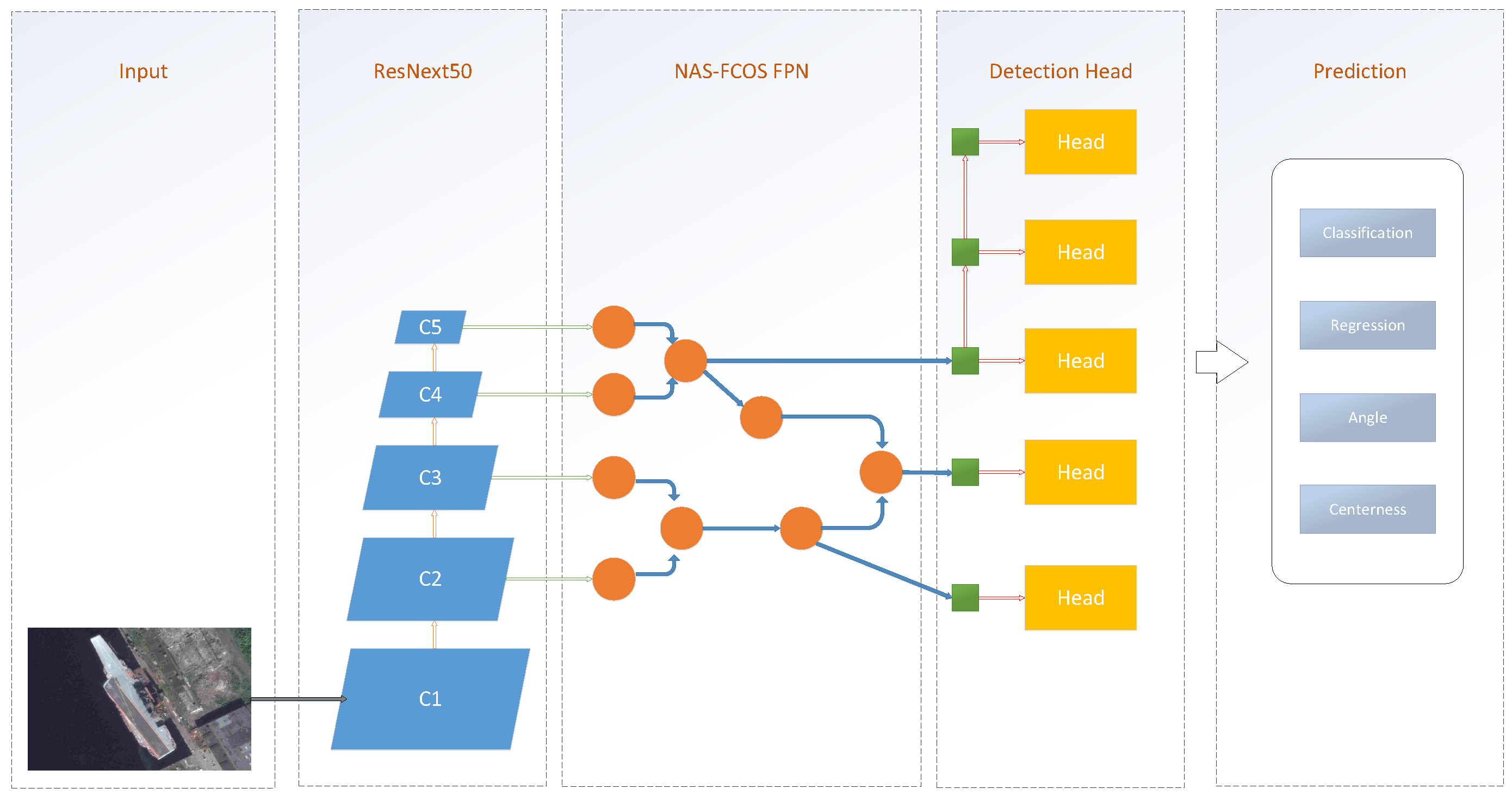
As shown in Figure 1, the CPS-Det can be divided into three components: the backbone network for feature extraction, the Feature Parymid Network (FPN) [16] for further feature representation, the refined detection head for final prediction and the postprocessing for train or test.
2.1.1. Feature Extraction
The backbone network of CPS-Det uses ResNeXt [17], which performs well in target detection. The ResNeXt network is an improvement on the Residual Neural Network (ResNet) [18], which was introduced in 2015 and won first place in the ImageNet competition classification task. The traditional method to improve the accuracy of the model is to deepen or widen the network. However, with the increase of the number of hyperparameters (such as the number of channels, filter size, etc.), the difficulty of network design and computational overhead will also increase. By modifying the topology of the submodules, ResNext can improve the accuracy without increasing the parameter complexity and also reduce the number of hyperparameters. The structure of ResNeXt is shown in Table 1.
2.1.2. Feature Fusion
Next, we input the feature map into the feature fusion network, which is named NASFCOS-FPN [19]. Instead of the traditional, hand-crafted approach, NASFCOS-FPN made full use of neural architecture search with reinforcement learning [20].
Neural architecture search with reinforcement learning is used to train a controller to select the best model structure in a given search space. It was proposed by NAS-FPN [21]. Based on Neural Architecture Search (NAS) with reinforcement learning, NAS-FPN designed a new controller. The controller uses the accuracy of the submodel in the search space as the reward signal to update the parameters. Thus, through such trial and error, the controller learns better structure, and the search space plays an important role in the successful search of the architecture.
NASFCOS-FPN uses NAS to design FPN for FCOS. It designs a series of selectable filters as the search space, and uses the NAS to select the filters and the connection mode. The FCOS network is trained with such a search strategy, and the FPN obtained is shown in the Figure 1. In COCO dataset [9], compared with FCOS, FCOS with NASFCOS-FPN improved by 2.4% in AP.
2.1.3. Prediction
The output of the feature fusion network will be input to the classification branch network, the localization branch network and the centerness branch network.
The classification branch network will predict the confidence of each point on the feature maps of different scales. This confidence determines the probability that the point belongs to a target.
The localization branch network is divided into BBox location branch and angle branch. The BBox location branch outputs the target outer rectangular box position predicted by each point on the feature maps of different scales. The angle branch outputs the target direction predicted by this point. The two branch networks predict the oblique rectangle position of the target together.
The centerness branch network outputs the distance between the point on the feature maps and the center of the target, ranging from 0 to 1. The higher the value, the closer the point is to the center.
2.1.4. Postprocessing
In the training stage, the output of the classification branch, the localization branch and the centerness branch will be used to calculate the classification loss, the BBox reg loss, the Angle Loss and the centerness loss.
In the test stage, points with high confidence in both classification branch and centerness branch will be screened out and their corresponding location output in localization branch will be obtained. After non-maximum suppression (NMS), the final prediction result is obtained.
2.2. Location Regression
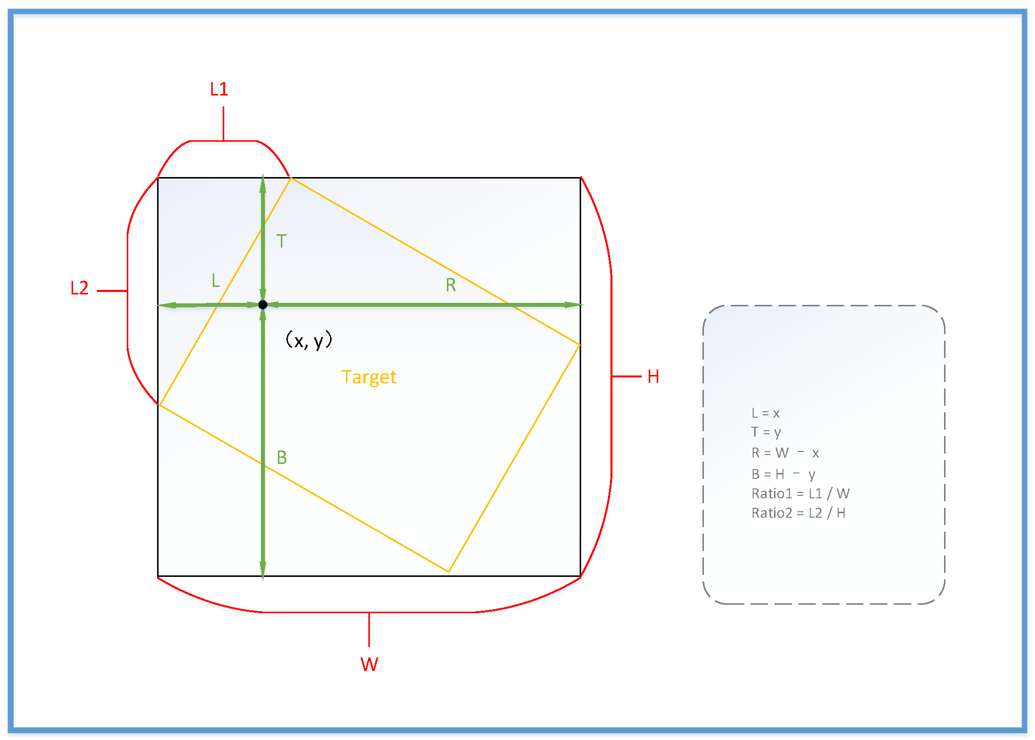
In the input part of the network, we processed the position of the target as shown in the Figure 2. First, we calculate the target’s BBox (xmin, ymin, xmax, ymax) based on its RBox (x-center, y-center, w, h, ). Secondly, we calculate the intersection point of target’s RBox and BBox on the top and left side of the vertex. Then we calculate the horizontal and vertical distances between these two intersection points and the upper left vertex of the BBox (L1, L2) and normalize them with W and H to get (Ratio1, Ratio2). In this representation, each oblique rectangle has a unique coordinate (xmax, ymax, xmin, ymin, ratio1, ratio2), which is free from periodic interference by angles. Finally, for each point on the feature maps, if it is within the target’s BBox, we calculate its distance to the four boundaries of the BBox (L, T, R, B). In this way, the input (L, T, R, B, Ratio1, Ratio2) our network accepts is actually the target’s external BBox and two parameters converted by angle of target. To facilitate subsequent calculations, we also input the angle of the target. However, it does not participate in the calculation of loss to avoid interference caused by angle periodicity.
2.3. Positive Sample Screening
After using the marking method of BBox + ratio, a large portion of the background points that do not belong to ships will be introduced into positive samples. This is due to the ship’s slender shape. Inspired by FCOS, we define that the few points that are closer to the center of the target predict a result that is closer to the actual location of the target. Therefore, the following methods were used to screen the positive samples. It can be visualized in Figure 3.
2.3.1. Scale Limit of BBox
We use the scheme of FCOS to directly limit the range of bounding box regression for each level of feature maps. For the 5 outputted feature maps, we set 5 intervals at each interval of (0, 64, 128, 256, 512, ). For the feature point inside the BBox of the target, its distance to the four edges is (L, T, R, B). If Min (L, T, R, B) or Max (L, T, R, B) is not in the corresponding value range of the feature map to which the feature point belongs, the feature point will no longer be regarded as a positive sample. As shown in Figure 3, in the loss calculation of a feature map, since the size of ShipA does not belong to the scale interval corresponding to this feature map, all points in the region where it is located are not considered as positive samples.
2.3.2. Defined Centerness
For the positive samples obtained after the above multi-scale screening, the centerness weight was calculated and the second screening was performed.
In FCOS, the weight of feature points is calculated by the following formula:
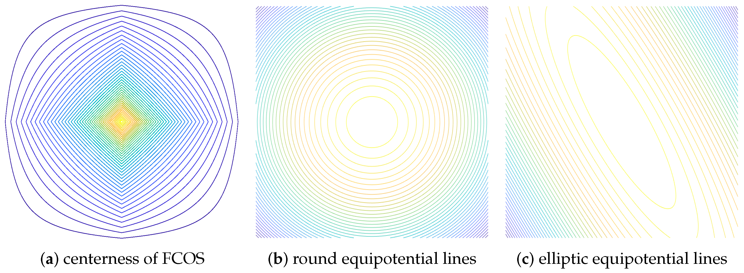
According to Figure 2, represents the distance between the target and the four boundaries of the BBox. This formula intuitively reflects the degree of deviation between the feature point and the target center. However, the weight distribution constituted by feature points is shown in the Figure 4a. It does not have uniform equipotential lines.
Based on the extraction of image features by convolutional network, within the target range, the closer the feature points are to the target center, the higher the weight of their prediction results will be. For a target, feature points that are equally distant from the center should be equally weighted. With the center point of the target as the origin, the distribution of feature points with the same weight will present a circular equipotential line, as shown in Figure 4b. It is a better choice to replace the centerness of FCOS with the following formula:
is the position of the feature point corresponding to the target center as the origin, and w and h are the width and height of the target’s BBox. On that basis, due to the particularity of the ship shape, the effective information on both sides of the ship is less than the direction of the ship’s head and tail. Therefore, the distribution of equipotential lines of feature points should be elliptical.
On the basis of the circular isopotential lines, we modify the ratio of the semi-major axis to the semi-minor axis, and rotate the coordinate system according to the direction angle of the target; we establish the following elliptic equation:
is the direction angle of the target, and k is the ratio of the semi-major axis to the semi-short axis of the ellipse. In this formula the distribution of the ellipse equipotential lines is close to the real shape of the target. Finally, the weights of feature points are shown as Figure 4c.
In order to approach the true length-width ratio of the ship, we set the hyperparameter k = 4. In this way, the weight of some feature points in the BBox will be negative, and most of them are concentrated on the sides and boundary of the ship.
2.3.3. Feedback to Localization and Classification
The centerness we calculated will be used for classification prediction and localization prediction. For localization prediction, we take centerness as the weight calculated by BBox reg loss and Angle Loss, so that feature points with more effective information can have higher prediction confidence. For classification prediction, we return the feature points with non-zero weight in centerness, and they are regarded as positive samples to participate in the loss calculation. As shown in Figure 3, The distribution of positive samples filtered by centerness will form an ellipse according to the direction of the target, rather than the rectangle that fills the entire target’s BBox. Different from localization prediction, classification prediction takes the weight of centerness as a classifier, and the value of weight itself does not participate in loss calculation.
In the rotation target detection method, GRS-Det [22], proposed by Zhang of Xidian University, it first determines whether the feature points are within the RBox of the target through geometric calculation, and then carries out weight calculation for each point. By contrast, we simplify the process with this feedback mechanism. The method proposed in this article does not need to establish a coordinate system in the feature map to determine the attribution of each point. Moreover, we can also adjust the ellipse hyperparameter k to control the proportion of positive samples to optimize the model of CPS-Det.
2.4. Loss Function
During the training stage, the loss function can be represented as the sum of classification loss, BBox reg loss, Angle Loss and centerness loss.
The definition of total loss is as follows:
represent Classification Loss, BBox Reg Loss, Angle Loss and Centerness Loss. are used to balance the importance of the four terms.
- Classification Lossdenotes the number of positive samples, represents Focal Loss [23], is the classification scores of each feature point on each feature map, is the correspondence of the real information of the ground truth on the feature map.
- BBox Reg Lossis the IOU Loss [24], is the centerness of each feature point calculated by elliptic equipotential line. is the prediction of BBox. is BBox’s real location.
- Angle Lossand is the two predicted ratios (Ratio1, Ratio2) used to calculate the direction angle of the target, and is the ratios calculated from the real angle of the target.In CPS-Det, the predicted angle of the target is calculated by:W and H are the width and height of target’s BBox. Therefore, as the angle approaches or , r1 or r2 approaches 0. In this case, the small error of r will also have a big impact on the calculation of the angle. To solve this problem, we improved SmoothL1 Loss from:to:Because of regulation of , Angle Loss has greater weight when the target direction is horizontal or vertical. This enables the network to make better optimization of the value boundary.
- Centerness Lossis Cross entropy loss. c is the predicted centerness and is the real centerness.
2.5. Summary of Algorithm Design
In this article, we use the anchor-free based deep learning network as the framework and propose an original strategy of positive sample screening based on the this network structure. In the process of prediction and postprocessing, a series of solutions are designed to serve this strategy.
First, we put forward the annotation method in the form of (L, T, R, B, Ratio1, Ratio2). In position regression, this method transforms the solution of RBox into the solution of BBox. In addition to simplifying the operation, it also lays a foundation for positive sample screening.
Second, we use the Scale limit of BBox proposed by FCOS. In FCOS, it is proposed to better detect the small target inside the big target. It allows objects of different sizes to belong to different feature maps. In ship detection of remote sensing images, there is usually no overlap of targets. However, the use of the Scale limit of BBox makes each target no longer belong to the whole feature map; it reduces redundant prediction tasks at each feature map, which improves the prediction accuracy of each feature map.
Third, we propose the centerness calculated by the ellipse equipotential lines. Since the elliptical equipotential lines are intended to approximate the shape of the ship, the centerness value of the pixel inside the ship is larger. The centerness calculated in this step can effectively clear the background around the ship.
Finally, in loss calculation, we take centerness as the weight, which makes the positive sample points with high quality have higher confidence. In order to compensate for the error in the calculation of horizontal and vertical ships’ angles caused by the annotation method proposed in the first step, we put forward an Angle Loss calculation method to correct the error.
3. Experimental Results and Discussions
3.1. Dataset and Evaluation Metrics
The HRSC2016 dataset [25] was used in the following experiment; it consists of two scenarios, inshore ship and offshore ship, which are derived from six well-known harbors. Image sizes range from to . The training, validation and test datasets consist of 436, 181 and 444 images, respectively.
The HRSC2016 dataset has a number of typical ship distributions, including inshore docking, side-by-side docking and docking in shipyards. In the traditional ship detection methods, the detection of ships docked inshore and docked in shipyard is usually a difficult problem. In this scenario, the characteristics of ships are difficult to distinguish from runways and containers. Meanwhile, the intensive docking of ships not only adds a lot of difficulties to the traditional target segmentation algorithm but also to many current deep learning methods. Therefore, the detection results on HRSC2016 dataset can directly reflect the response ability of target detection network to complex scenes.
In order to evaluate the effectiveness of the network, we use recall rate, average precision (AP) and computing speed as the evaluation criteria.
3.2. Experimental Environment
In this article, all the experiments are implemented under the Pytorch framework. On HRSC2016 dataset, each input image was resized to . The network is trained on single Nvidia GeForce RTX 2080Ti, and the batch size is set to 4. In the experiment, the size of the input training image is , and the ResNext50 network was used.
We use the FCOS network as baseline, initialized with the ResNext50 pre-training matrix, and the usual FPN to fuse features. In the subsequent training, the training results of FCOS are used as initialization. The number of epochs in training is 50, and the initial learning rate is 0.01. In each epoch, it is one iter to complete a training of all images within a batch, and one epoch is completed after all images are trained. In order to achieve better convergence of network training, the learning rate was of the initial learning rate in the first 500 iters, and then the learning rate was restored to 0.01. The learning rate at 60% and 80% of the training process decays to of the current learning rate. In the experiment initialized with FCOS, the number of training epochs dropped to 40. In each epoch, each image goes through ten iterations with random flips, rotations, changes in brightness and other data augmentations to increase the robustness of the detector.
3.3. Ablation Study
In this experiment, in order to obtain a more accurate comparison effect, we use Equation (2) to calculate the centerness in the experiment using FCOS as baseline. In order to test the results of positive sample screening, we conducted the following experiments:
- (1)
- Firstly, we experiment the effect of the limit on the regression size of the bounding box on the results. After the restriction of BBox’s scale was removed, the positive samples of each feature layer increased significantly. In the process of training, loss declines slowly. When the pre-training matrix uses ResNext50 to train the same epoch, loss does not decline to the minimum value. It also gets a bad result in validation. The experimental results are shown in the Figure 5. In this experiment, a total of 617 images were trained, and they go through ten iterations to augment the data. In the training of 50 epochs, a total of 77,000 iters were executed while batch = 4. The calculation of Loss is shown in Equation (4). All of the are equal to 1. Without limiting range of BBox, it only got a AP value of 0.601, and tests showed that it did not capture the ship’s characteristics. The experiment proves that the large increase of positive samples has a negative effect when the size restriction of BBox is canceled.
- (2)
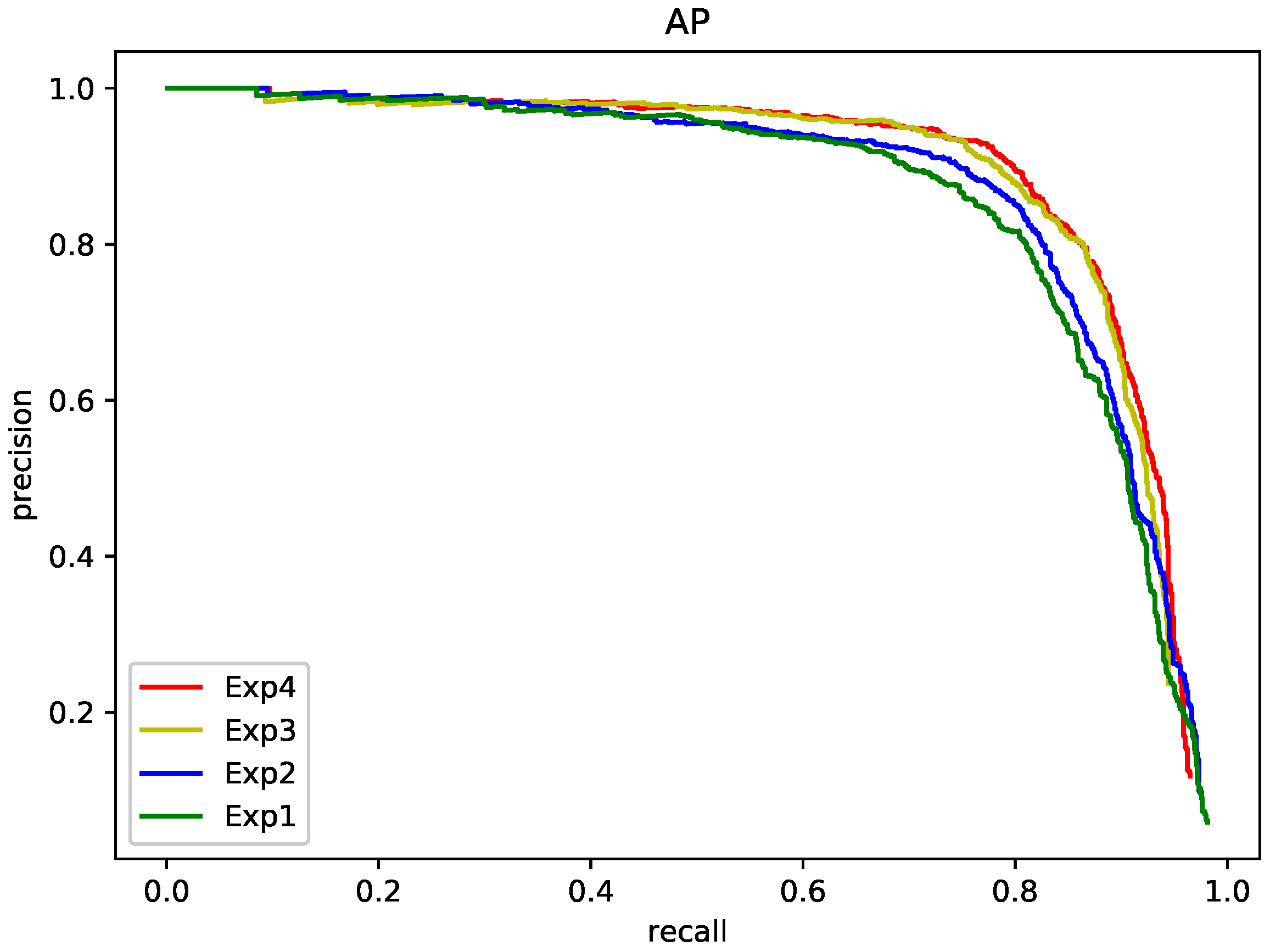
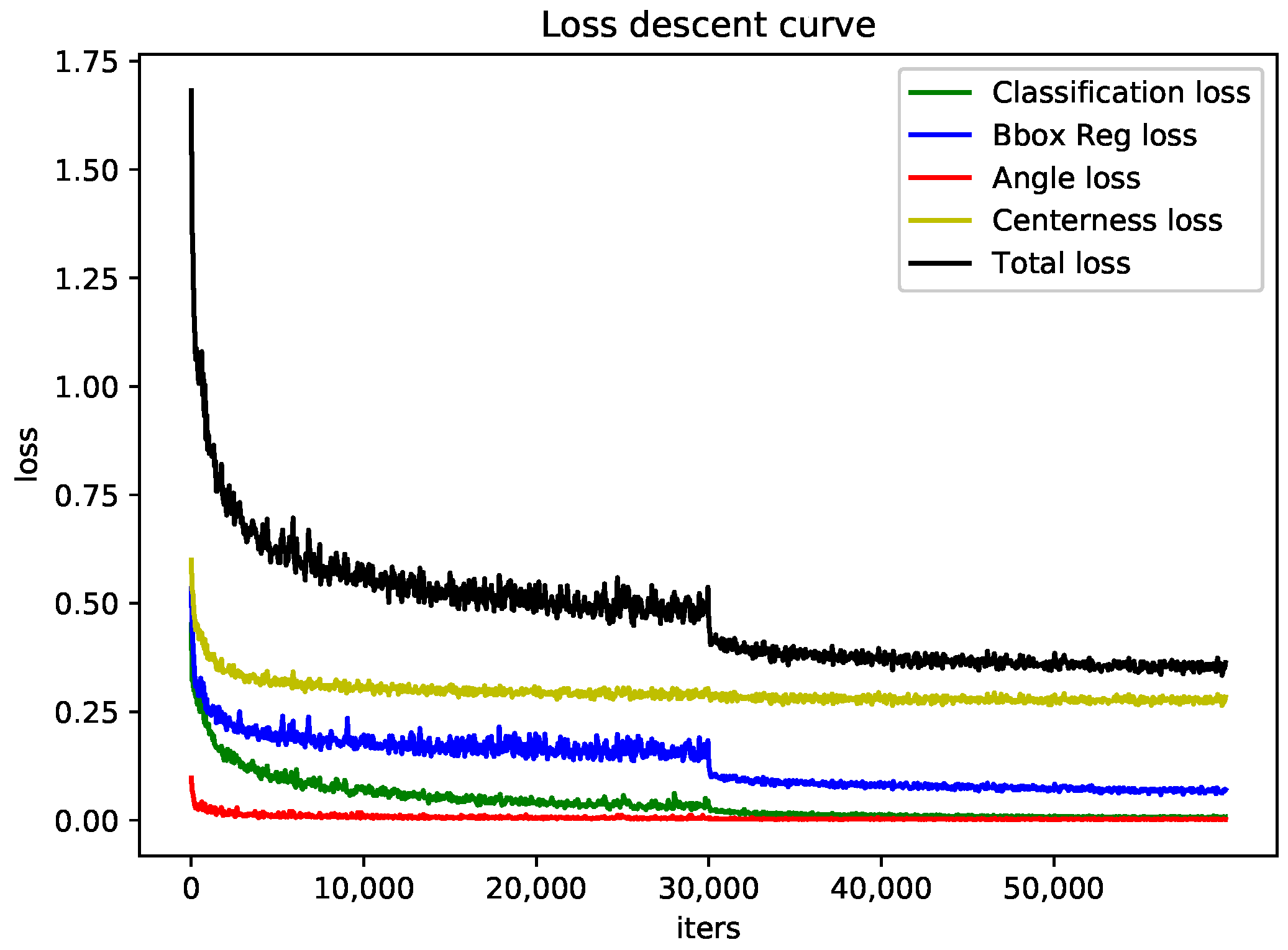
- Next, the influence of elliptic equipotential line feature screening and NASFCOS-FPN on the experimental results is tested. Recall-Precision curve are shown in Figure 6. In Figure 6, (Exp1, Exp2, Exp3, Exp4) corresponds to Table 2. By integrating the curves in the figure, we get the AP of the different methods. As shown in Table 2, elliptic equipotential line screening can improve the results. It improves the AP of baseline by 1.92%. This also reached a consistent result with the first experiment, which is that reducing the inferior positive sample points helps to improve the network’s ability to acquire target features. At the same time, we tested the effect of NASFCOS-FPN on the results. We introduce NASFCOS-FPN to optimize the feature fusion, which can enable the retained positive sample points to obtain more reliable feature information. It improves AP of baseline by 2.42%. Finally, we combine the two approaches; the AP was improved to 0.891. Furthermore, this is the complete structure of CPS-Det. Its loss curve is shown in the Figure 7. Training based on the baseline executed only 40 epochs, giving a total of about 60,000 iters.
- (3)
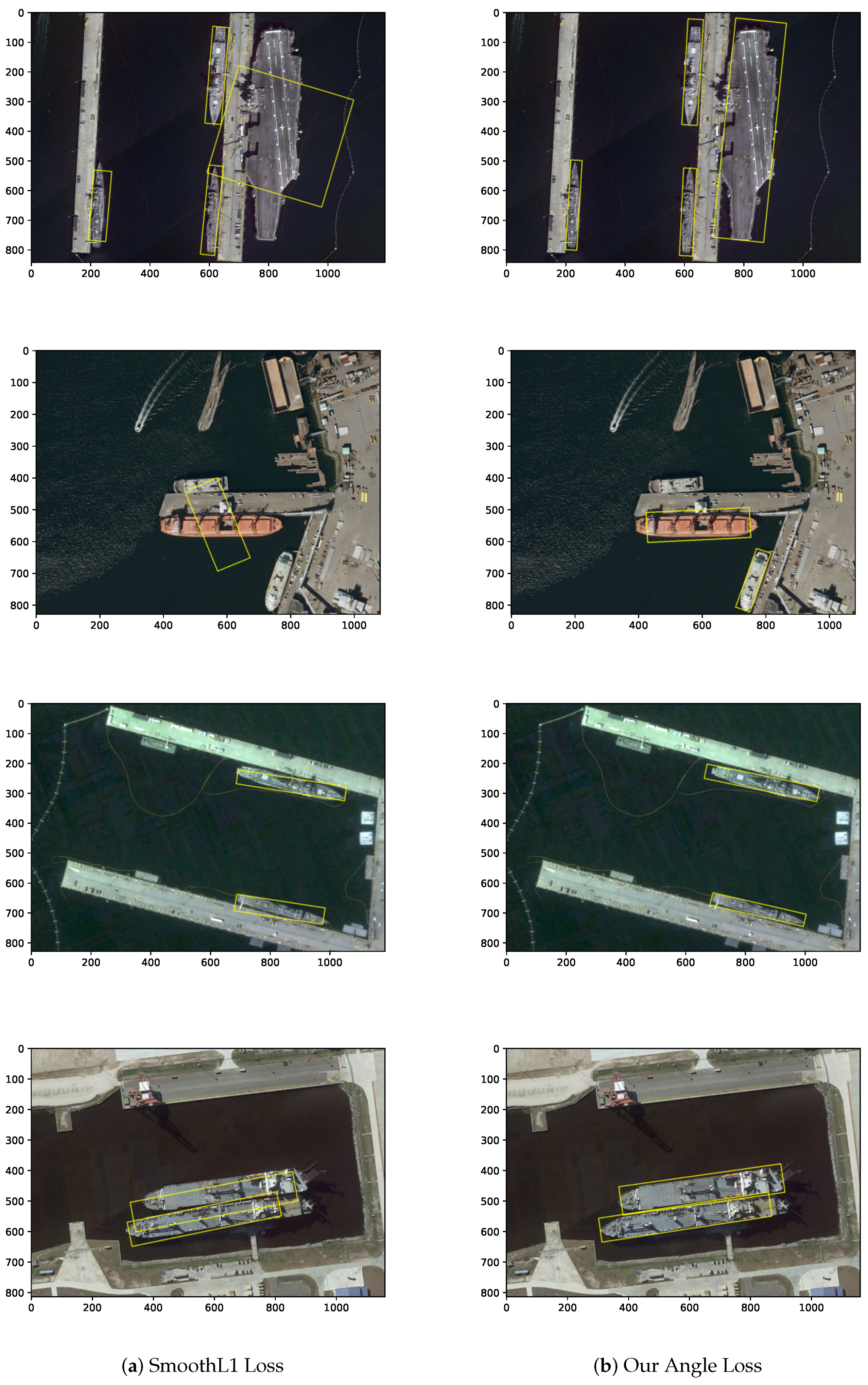
- The following experiment compared the results using improved scheme in the calculation of Angle Loss and using SmoothL1 Loss. According to Equation (11), we use to control weight of Angle Loss when . Experimental results have proven that we have better detection results on both horizontal and vertical ships compared to using SmoothL1 Loss directly. The results of the detection are shown in Figure 8. Figure 8a is the result of using SmoothL1 Loss, and Figure 8b is the result of using Angle Loss defined by us. We can see that in the horizontal and vertical cases, the accuracy of angle detection is improved, and the problem of missed detection caused by angle error is also improved.
- (4)
- We conducted a series of experiments as shown in Table 3 below to verify the influence of the ellipse parameter k. As k increases, the positive sample will decrease as the ellipse contracts, and the weight of all positive sample points except the center point will also decrease. AP is going to increase as k goes up, but the growth rate is also decreasing. This means that valid positive samples have been screened out, and the further increase of k will only lead to the imbalance of positive and negative samples, which finally leads to the decline of AP.
3.4. Result on HRSC2016
To demonstrate the performance of CPS-Det, we compared it with some state-of-the-art models, i.e., Gliding Vertex [26], Det [27], IENet [28], FCOS [8] and GRS-Det [22]. The overall comparison performance is reported in Table 4. It can be noted that the performance of CPS-Det on AP is better than that of Gliding Vertex using the similar labeling method and GRS-Det also using the anchor-free method. It is inferior to the Det by 0.14%, which uses deeper layers on backbone. This shows that CPS-Det has advanced performance in ship detection. Considering the accuracy and speed, CPS-Det still achieves excellent results. As shown in Table 5, because the network is based on the anchor-free design and has strict criteria for the selection of positive samples, it takes a short detection time on each image. On the RTX2080 with TFLOPS 8.98% lower than the GTX1080Ti, our time is 6.39% longer than the GRS-Det. On the RTX2080Ti with TFLOPS 21.57% higher than the GTX1080Ti, our time is 22.52% shorter than the GRS-Det. In order to getting more intuitive comparison of processing speed on different platforms, we propose the following formula to evaluate the speed:
The speed calculated by this formula represents the processing speed per unit of time and unit of computing force.
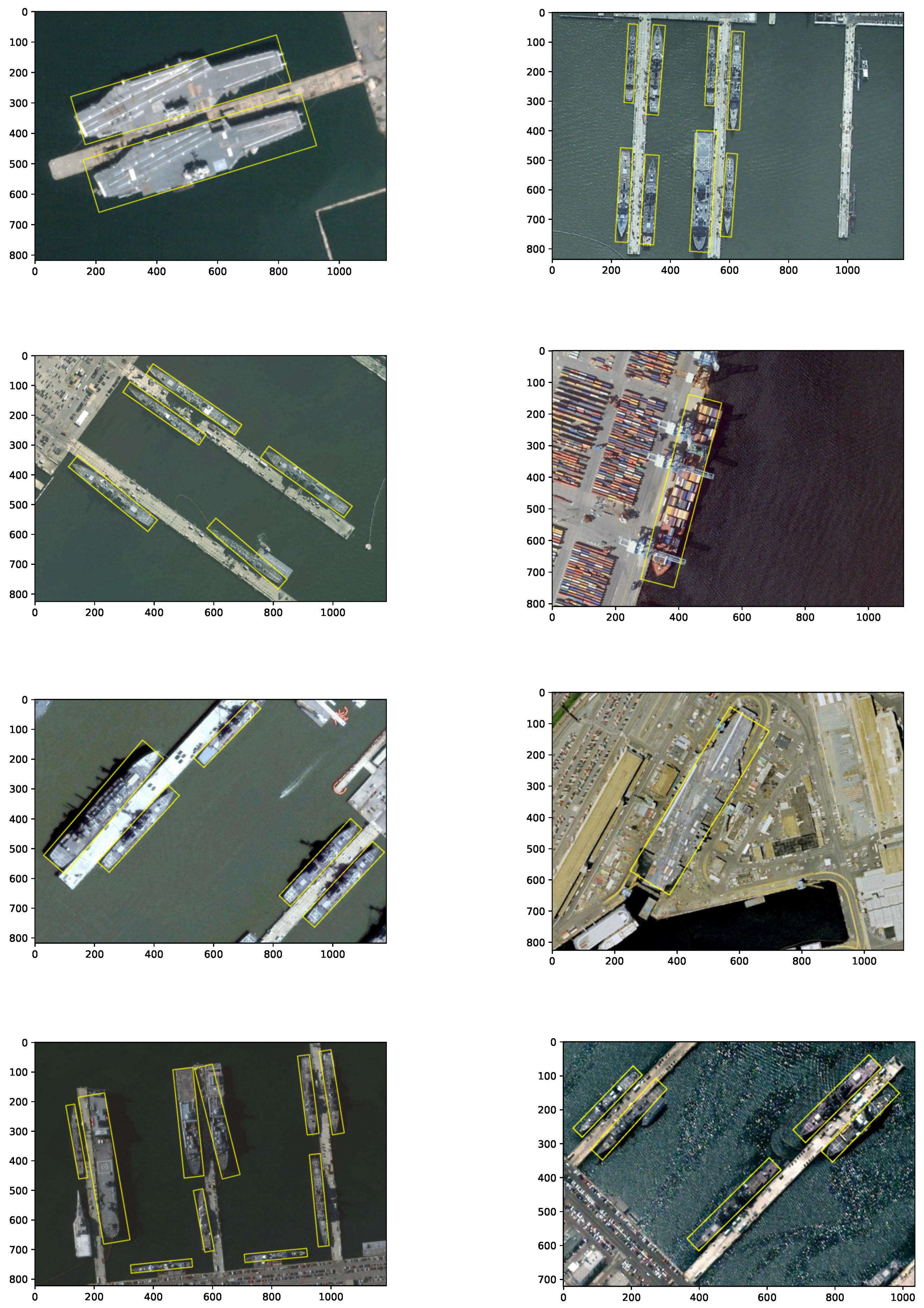
To further show the performance of CPS-Det, the detection results are visualized in Figure 9. According to the detection results, CPS-Det has a good detection effect for different imaging sources, different sizes and different types of ships. This result also confirms the improvement effect of the ellipse parameter k = 4 on the detection accuracy, because it approximates the aspect ratio of the ship. CPS-Det can accurately detect targets in the presence of dense arrangement and the interference of suspected targets on land. Even if the ship is surrounded inside the land, the network can detect it through the target characteristics obtained by training. This proves the robustness of the detector.
3.5. Discussion
In this article, we discuss how positive sample screening can improve the detection performance of achor-free based networks. Based on this idea, we improved the labeling method of the target, the weight distribution of the positive sample and the calculation method of Angle Loss. Through these methods, the performance of CPS-Det has been greatly improved.
Compared with the anchor-based method, our thinking is obviously different. In general, we believe that more scale anchors, deeper networks and more samples can be used to obtain more accurate prediction detectors. However, the opposite conclusion was drawn in the experiment above, that is, screening out a small number of high-quality positive samples has a positive impact on the detection accuracy. In our analysis, it is believed that the anchor-based method realizes the gradient distribution from far to near distance and from low to high overlap degree by matching the anchors and ground truth of each feature point. Even if the feature point is not in the region that the target belongs to, some of its anchors will form a good match to the target location. In the training, they point to the real position of the target together through positional regression. In the anchor-free based detector, however, each feature point has only one chance to predict its distance from the target boundary. This makes it difficult to form a dense gradient but will lead to a part of the background near the target to give the wrong prediction results, affecting the accuracy of detection. Therefore, under the condition of positive and negative sample equilibrium, keeping effective positive sample points can significantly improve the accuracy and reduce the computation.
Based on the above conclusion, we arrive at a paradoxical fact: in a sense, increasing or decreasing the number of positive samples both improve the target detection result. The root cause of this paradox is not whether or not we use anchor-free based network but the feature point-based convolutional network itself. We give each feature point a variety of detection tasks, such as target classification, position, angle, etc. In the end, these tasks are performed by a feature point with the highest confidence probability. This is contrary to our common sense. In the process of human target recognition, the type of target is usually determined by the central region. The outline of a target, on the other hand, is determined by its edges. Based on this difference, we come to this conclusion: whether using anchor-free based network or anchor based network, the purpose of positive sample selection is to reach a critical point, so that a single feature point can obtain the most accurate prediction for multiple tasks. How to make full use of the target information in the image to achieve real intelligent recognition is still a complex and important subject.
There are still some aspects of the experiment above worth discussing:
- Under the limited scale of BBox, although the detection accuracy has been improved, the feature maps in the middle lose the chance to predict small targets and large targets. In the detection of large targets, because its aspect ratio is close to the setting of ellipse hyperparameter k, it still has good detection results. However, in small target detection, the performance of the detector is reduced.
- Although our improved Angle Loss optimizes the detection results of horizontal and vertical targets, it does not fundamentally solve this problem. This is because the angle is not predicted directly but calculated by trigonometric functions. As we approach the boundary value, the error will affect the result more than we can adjust it by weight. This can lead to angles that are not correctly predicted over a very small interval. Furthermore, what we did was compress this interval to improve the overall prediction accuracy. We tried to give more weight to the loss calculation close to the boundary value, but this would lead to the inability to find the direction of gradient descent in training.
These are the problems that we will try to solve in future research.
4. Conclusions
The experiment designed in this article achieves directional target detection based on anchor-free network. On HRSC2016 dataset, CPS-Det has excellent detection accuracy and faster detection speed. The annotation scheme proposed by us solves the periodicity problem of angle in training. A series of subsequent positive sample screening based on this scheme not only reduces the complex geometric operations but also reduces the number of samples in which the network participates in the prediction.
At present, CPS-Det is proposed for ship detection and also makes a specific target matching scheme for this purpose. In the task of ship detection, these proposed schemes are proved to be effective.
Different from the field of computer vision, under the limitation of resolution of remote sensing images, the features of targets are fewer and simpler, mainly manifested as simple geometric figures. Therefore, the scheme of assigning sample weights according to target characteristics proposed in this paper can also be transferred to other related fields. For example, the elliptical equipotential line scheme proposed in this paper can also be applied to high tower detection or airport runway detection. Furthermore, the idea of modeling the shapes for different types of targets can also be applied to the recognition and classification of multiple targets in complex scenes.
In the future, we will apply it to more areas of remote sensing target recognition and achieve higher accuracy and wider applications.
Author Contributions
Y.Y. and Z.P. designed the algorithm; Y.Y. performed the algorithm with Python; C.D. and Y.H. guided whole project containing this one; Y.Y. and Z.P. wrote this paper; Z.P. read and revised this paper. All authors have read and agreed to the published version of the manuscript.
Funding
This research received no external funding.
Institutional Review Board Statement
Not applicable.
Informed Consent Statement
Not applicable.
Data Availability Statement
Publicly available datasets were analyzed in this study. This data can be found here: https://aistudio.baidu.com/aistudio/datasetdetail/31232.
Conflicts of Interest
The authors declare no conflict of interest.
References
- Liu, W.; Anguelov, D.; Erhan, D.; Szegedy, C.; Reed, S.; Fu, C.Y.; Berg, A.C. SSD: Single Shot MultiBox Detector; Springer: Cham, Switzerland, 2016. [Google Scholar]
- Ren, S.; He, K.; Girshick, R.; Sun, J. Faster R-CNN: Towards Real-Time Object Detection with Region Proposal Networks. IEEE Trans. Pattern Anal. Mach. Intell. 2017, 39, 1137–1149. [Google Scholar] [CrossRef] [PubMed] [Green Version]
- Redmon, J.; Farhadi, A. YOLOv3: An Incremental Improvement. arXiv 2018, arXiv:1804.02767. [Google Scholar]
- Law, H.; Deng, J. CornerNet: Detecting Objects as Paired Keypoints. In Proceedings of the European Conference on Computer Vision (ECCV), Munich, Germany, 8–14 September 2018; pp. 734–750. [Google Scholar]
- Zhou, X.; Zhuo, J.; Krahenbuhl, P. Bottom-Up Object Detection by Grouping Extreme and Center Points. In Proceedings of the 2019 IEEE/CVF Conference on Computer Vision and Pattern Recognition (CVPR), Long Beach, CA, USA, 16–20 June 2019. [Google Scholar]
- Zhou, X.; Wang, D.; Krhenbühl, P. Objects as Points. arXiv 2019, arXiv:1904.07850. [Google Scholar]
- Kong, T.; Sun, F.; Liu, H.; Jiang, Y.; Shi, J. FoveaBox: Beyond Anchor-based Object Detector. IEEE Trans. Image Process. 2020, 29, 7389–7398. [Google Scholar] [CrossRef]
- Tian, Z.; Shen, C.; Chen, H.; He, T. FCOS: Fully Convolutional One-Stage Object Detection. In Proceedings of the 2019 IEEE/CVF International Conference on Computer Vision (ICCV), Seoul, Korea, 27 October–2 November 2019. [Google Scholar]
- Lin, T.Y.; Maire, M.; Belongie, S.; Hays, J.; Zitnick, C.L. Microsoft COCO: Common Objects in Context. In Proceedings of the European conference on computer vision (ECCV), Zürich, Switzerland, 6–12 September 2014. [Google Scholar]
- Wang, J.; Lu, C.; Jiang, W. Simultaneous Ship Detection and Orientation Estimation in SAR Images Based on Attention Module and Angle Regression. Sensors 2018, 18, 2851. [Google Scholar] [CrossRef] [PubMed] [Green Version]
- Chen, C.; He, C.; Hu, C.; Pei, H.; Jiao, L. MSARN: A Deep Neural Network Based on an Adaptive Recalibration Mechanism for Multiscale and Arbitrary-oriented SAR Ship Detection. IEEE Access 2019, 7, 159262–159283. [Google Scholar] [CrossRef]
- Jiang, Y.; Zhu, X.; Wang, X.; Yang, S.; Li, W.; Wang, H.; Fu, P.; Luo, Z. R2CNN: Rotational Region CNN for Orientation Robust Scene Text Detection. arXiv 2017, arXiv:1706.09579. [Google Scholar]
- Yang, X.; Yang, J.; Yan, J.; Zhang, Y.; Zhang, T.; Guo, Z.; Xian, S.; Fu, K.S. Towards More Robust Detection for Small, Cluttered and Rotated Objects. arXiv 2018, arXiv:1811.07126. [Google Scholar]
- Xia, G.S.; Bai, X.; Ding, J.; Zhu, Z.; Belongie, S.; Luo, J.; Datcu, M.; Pelillo, M.; Zhang, L. DOTA: A Large-scale Dataset for Object Detection in Aerial Images. In Proceedings of the 2018 IEEE/CVF Conference on Computer Vision and Pattern Recognition, Salt Lake City, UT, USA, 18–22 June 2018. [Google Scholar]
- Zhu, H.; Chen, X.; Dai, W.; Fu, K.; Ye, Q.; Jiao, J. Orientation robust object detection in aerial images using deep convolutional neural network. In Proceedings of the IEEE International Conference on Image Processing, Quebec, QC, Canada, 27–30 September 2015. [Google Scholar]
- Lin, T.Y.; Dollar, P.; Girshick, R.; He, K.; Hariharan, B.; Belongie, S. Feature Pyramid Networks for Object Detection. In Proceedings of the 2017 IEEE Conference on Computer Vision and Pattern Recognition (CVPR), Honolulu, HI, USA, 21–26 July 2017. [Google Scholar]
- Xie, S.; Girshick, R.; Dollár, P.; Tu, Z.; He, K. Aggregated Residual Transformations for Deep Neural Networks. In Proceedings of the IEEE Conference on Computer Vision and Pattern Recognition (CVPR), Honolulu, HI, USA, 21–26 July 2017. [Google Scholar]
- He, K.; Zhang, X.; Ren, S.; Sun, J. Deep residual learning for image recognition. In Proceedings of the IEEE Conference on Computer Vision and Pattern Recognition, Las Vegas, NV, USA, 26 June–1 July 2016; pp. 770–778. [Google Scholar]
- Wang, N.; Gao, Y.; Chen, H.; Wang, P.; Tian, Z.; Shen, C.; Zhang, Y. NAS-FCOS: Fast neural architecture search for object detection. In Proceedings of the IEEE/CVF Conference on Computer Vision and Pattern Recognition, Virtual, 14–19 June 2020; pp. 11943–11951. [Google Scholar]
- Zoph, B.; Le, Q.V. Neural Architecture Search with Reinforcement Learning. arXiv 2016, arXiv:1611.01578. [Google Scholar]
- Ghiasi, G.; Lin, T.Y.; Le, Q.V. NAS-FPN: Learning Scalable Feature Pyramid Architecture for Object Detection. In Proceedings of the 2019 IEEE/CVF Conference on Computer Vision and Pattern Recognition (CVPR), Long Beach, CA, USA, 16–20 June 2019. [Google Scholar]
- Zhang, X.; Wang, G.; Zhu, P.; Zhang, T.; Li, C.; Jiao, L. GRS-Det: An Anchor-Free Rotation Ship Detector Based on Gaussian-Mask in Remote Sensing Images. IEEE Trans. Geosci. Remote Sens. 2020. [Google Scholar] [CrossRef]
- Lin, T.Y.; Goyal, P.; Girshick, R.; He, K.; Dollár, P. Focal loss for dense object detection. In Proceedings of the IEEE International Conference on Computer Vision, Venice, Italy, 22–29 October 2017; pp. 2980–2988. [Google Scholar]
- Yu, J.; Jiang, Y.; Wang, Z.; Cao, Z.; Huang, T. Unitbox: An advanced object detection network. In Proceedings of the 24th ACM International Conference on Multimedia, Amsterdam, The Netherlands, 15–19 October 2016; pp. 516–520. [Google Scholar]
- Liu, Z.; Yuan, L.; Weng, L.; Yang, Y. A high resolution optical satellite image dataset for ship recognition and some new baselines. In Proceedings of the International Conference on Pattern Recognition Applications and Methods, Porto, Portugal, 24–26 February 2017; Volume 2, pp. 324–331. [Google Scholar]
- Xu, Y.; Fu, M.; Wang, Q.; Wang, Y.; Bai, X. Gliding vertex on the horizontal bounding box for multi-oriented object detection. IEEE Trans. Pattern Anal. Mach. Intell. 2019. [Google Scholar] [CrossRef] [PubMed] [Green Version]
- Yang, X.; Liu, Q.; Yan, J.; Li, A.; Zhang, Z.; Yu, G. R3Det: Refined Single-Stage Detector with Feature Refinement for Rotating Object. arXiv 2019, arXiv:1908.05612. [Google Scholar]
- Lin, Y.; Feng, P.; Guan, J. IENet: Interacting Embranchment One Stage Anchor Free Detector for Orientation Aerial Object Detection. arXiv 2019, arXiv:1912.00969. [Google Scholar]
Figure 1.
Network of CPS-Det.

Figure 2.
The annotation form we defined of target’s RBox.

Figure 3.
The process of positive sample screening.

Figure 4.
The equipotential line of the weight distribution.

Figure 5.
Loss descent curve of baseline.

Figure 6.
AP curve of ablation study, "Exp" represents the experimental sequence number in Table 2.
Figure 6.
AP curve of ablation study, "Exp" represents the experimental sequence number in Table 2.

Figure 7.
Loss descent curve of CPS-Det.

Figure 8.
The effect of Angle Loss.

Figure 9.
Visualization of detection results from CPS-Det on HRSC2016 dataset.


Table 1.
The structure of ResNeXt50.
| Stage | Output | ResNeXt50 |
|---|---|---|
| conv1 | 112 × 112 | 7 × 7, 64, stride 2 |
| conv2 | 56 × 56 | 3 × 3, max pool, stride 2 |
| conv3 | 28 × 28 | |
| conv4 | 14 × 14 | |
| conv5 | 7 × 7 | |
| 1 × 1 | global average pool | |
| 1000-d fc, softmax | ||
| params | 25.0 | |
Table 2.
Ablation study of CPS-Det on HRSC2016.
| Model | NASFCOS-FPN | Equipotential Line | AP | No. |
|---|---|---|---|---|
| Baseline | No | No | 0.8578 | Exp1 |
| No | Yes | 0.8770 | Exp2 | |
| Yes | No | 0.8820 | Exp3 | |
| Yes | Yes | 0.8912 | Exp4 |
Table 3.
The influence of the ellipse parameter k.
| k | 1 | 2 | 4 | 6 | 8 |
|---|---|---|---|---|---|
| AP | 0.8820 | 0.8877 | 0.8912 | 0.8892 | 0.8764 |
Table 4.
Overall performance comparisons on HRSC2016 dataset.
| Model | Backbone | Anchor-Free | AP |
|---|---|---|---|
| IENet | ResNet101 | Yes | 0.7501 |
| FCOS (BBox) | ResNeXt50 | Yes | 0.8014 |
| Gliding Vertex | ResNet101 | No | 0.8820 |
| Det | ResNet101 | No | 0.8926 |
| GRS-Det | ResNet50 | Yes | 0.8890 |
| CPS-Det | ResNext50 | Yes | 0.8912 |
Table 5.
Average speed evaluation on different models.
| Model | AP | GPU | TFLOPS | Time | Speed |
|---|---|---|---|---|---|
| Det | 0.8926 | GTX1080Ti | 10.8 | 0.0833 s | 1.112 |
| GRS-Det (ResNet50) | 0.8890 | GTX1080Ti | 10.8 | 0.0595 s | 1.556 |
| CPS-Det | 0.8912 | RTX2080 | 9.83 | 0.0633 s | 1.615 |
| CPS-Det | 0.8912 | RTX2080Ti | 13.13 | 0.0461 s | 1.652 |
Publisher’s Note: MDPI stays neutral with regard to jurisdictional claims in published maps and institutional affiliations. |
© 2021 by the authors. Licensee MDPI, Basel, Switzerland. This article is an open access article distributed under the terms and conditions of the Creative Commons Attribution (CC BY) license (https://creativecommons.org/licenses/by/4.0/).
Share and Cite
MDPI and ACS Style
Yang, Y.; Pan, Z.; Hu, Y.; Ding, C. CPS-Det: An Anchor-Free Based Rotation Detector for Ship Detection. Remote Sens. 2021, 13, 2208. https://0-doi-org.brum.beds.ac.uk/10.3390/rs13112208
AMA Style
Yang Y, Pan Z, Hu Y, Ding C. CPS-Det: An Anchor-Free Based Rotation Detector for Ship Detection. Remote Sensing. 2021; 13(11):2208. https://0-doi-org.brum.beds.ac.uk/10.3390/rs13112208
Chicago/Turabian StyleYang, Yi, Zongxu Pan, Yuxin Hu, and Chibiao Ding. 2021. "CPS-Det: An Anchor-Free Based Rotation Detector for Ship Detection" Remote Sensing 13, no. 11: 2208. https://0-doi-org.brum.beds.ac.uk/10.3390/rs13112208
Note that from the first issue of 2016, this journal uses article numbers instead of page numbers. See further details here.