A Burned Area Mapping Algorithm for Sentinel-2 Data Based on Approximate Reasoning and Region Growing

Abstract

Sentinel-2 (S2) multi-spectral instrument (MSI) images are used in an automated approach built on fuzzy set theory and a region growing (RG) algorithm to identify areas affected by fires in Mediterranean regions. S2 spectral bands and their post- and pre-fire date (Δ_post-pre) difference are interpreted as evidence of burn through soft constraints of membership functions defined from statistics of burned/unburned training regions; evidence of burn brought by the S2 spectral bands (partial evidence) is integrated using ordered weighted averaging (OWA) operators that provide synthetic score layers of likelihood of burn (global evidence of burn) that are combined in an RG algorithm. The algorithm is defined over a training site located in Italy, Vesuvius National Park, where membership functions are defined and OWA and RG algorithms are first tested. Over this site, validation is carried out by comparison with reference fire perimeters derived from supervised classification of very high-resolution (VHR) PlanetScope images leading to more than satisfactory results with Dice coefficient > 0.84, commission error < 0.22 and omission error < 0.15. The algorithm is tested for exportability over five sites in Portugal (1), Spain (2) and Greece (2) to evaluate the performance by comparison with fire reference perimeters derived from the Copernicus Emergency Management Service (EMS) database. In these sites, we estimate commission error < 0.15, omission error < 0.1 and Dice coefficient > 0.9 with accuracy in some cases greater than values obtained in the training site. Regression analysis confirmed the satisfactory accuracy levels achieved over all sites. The algorithm proposed offers the advantages of being least dependent on a priori/supervised selection for input bands (by building on the integration of redundant partial burn evidence) and for criteria/threshold to obtain segmentation into burned/unburned areas.

1. Introduction

Wildfires are the largest contributor to global biomass burning (BB) and represent a significant dynamic component of ecosystems, affecting terrestrial and atmosphere systems [1,2]. In vegetated areas of Southern Europe, fire is a major damaging agent and recent years (2017–2018) have witnessed unprecedented fire seasons with countries suffering large forest fires as a consequence of drought and heatwaves. Global warming has been affecting fires with increased frequency and severity, as observed in both real and simulated data [3,4]; this effect is particularly true in Mediterranean ecosystems (object of this work) where, according to models’ forecasting, warming and a precipitation deficit will exacerbate fire weather conditions [5].

Fires impact on atmospheric chemistry, with aerosols and greenhouse gas emissions [6], the carbon budgets [7], hydrological cycles, soils and vegetation components of ecosystems [8,9]. In this framework, the extent of the area affected by fires is critical to investigate trends and patterns of fire occurrence and identify drivers of fire occurrence as well as for modeling future fire patterns and fire regimes; this information can therefore support the assessments of fire impacts on both natural and social systems. Several studies can be mentioned on the use of remote sensing (RS) to map burned areas at a regional to global scale [10,11,12]. Coarse-resolution RS data have been proved to be the most suitable source for depicting fire distribution over large areas and one primary image source for burned area (BA) products is the Moderate Resolution Imaging Spectrometer (MODIS) [13]. To the aim of improving accuracy of global estimates by detecting smaller fires (<50 ha), higher-resolution sensors have been exploited, such as 300 m Medium Resolution Imaging Spectrometer (MERIS) and 100 m Project for On-Board Autonomy–Vegetation (PROBA-V) [10,14,15], although the results were not always more accurate compared to coarser spatial resolution products [16].

At a regional scale and in heterogeneous environments, such as the Mediterranean ecosystems of Southern Europe, coarse-resolution data do not provide enough spatial detail and medium/high- and very high-resolution satellite images are preferable for accurately mapping burned areas. Indeed, small fires could significantly contribute to global effects of fires [15,17]. The greatest challenge in the RS community is the development of a global algorithm for mapping burned areas from decametric satellite images (e.g., Sentinel-2 and Landsat missions) [18,19,20], although important steps forward are shown by recent works [21,22]. In order to achieve this objective, some issues are yet to be addressed; among them a significant variability, across the ecosystems, of burned area spectral response as a function of pre-fire vegetation conditions and characteristics, fire behavior and intensity as well as time since the fire event. The lower revisiting time of medium spatial resolution satellites reduces the likelihood of observing burned surfaces immediately after the fire when spectral separability is greatest; yet Sentinel-2 (S2) revisiting time, obtained with the combined use of A&B missions, offers unprecedent opportunity with an average revisiting time of about five days [23].

Several algorithms have been proposed for mapping burned areas in the diverse ecosystems of the globe [12] and some key elements can be pointed out as providing the most robust approaches: supervised self-adaptive algorithms that can fit local conditions and contextual, multi-source (combining active fires) and multi-temporal approaches that can reduce the likelihood of commission errors due to spectral confusion with low albedo surfaces and highlight changes induced by fire on the surface [16,24,25].

The algorithm proposed here exploits the abovementioned key elements to deliver a semi-automatic robust and self-adaptive classification algorithm for S2 imagery exploiting pre-fire and post-fire acquisitions to maximize mapping accuracy. The algorithm inherits from the conceptual framework of the multi-criteria soft aggregation approach of burn evidence proposed by Stroppiana et al. (2012) [26] for burned area mapping and also applied for flooding mapping [27].

Major improvements with respect to the previous algorithm characteristics are (i) the use of S2 band reflectance in post-fire images and of their temporal difference between post- and pre-fire acquisitions and (ii) the definition of soft constraints by membership functions of fuzzy sets based on statistics (percentiles) of reflectance as derived from training areas. These improvements build on (i) the exploitation of a greater frequency of acquisition of S2 data (nominal five days when A and B constellations are combined), that allows the implementation of a robust change detection approach and (ii) a more automatic way for defining membership functions based on frequency distribution of training pixels over burned and unburned surfaces [19]. In particular, the algorithm aggregates partial evidence of burn, extracted from the information provided by S2 bands through the membership functions, into a synthetic score of global evidence by means of an ordered weighted averaging (OWA) operator [28]. Each S2 band could potentially and independently be used as a source of evidence of burn for the identification of areas affected by fires, hereafter named ‘partial evidence’ since it is given by a single input feature. However, the concurrent aggregation of multiple spectral bands can provide a more reliable evaluation of the occurrence of fires by modeling a convergence of evidence provided by redundant information, hereafter named ‘global evidence’ since it is given by multiple input features. This multi-criteria soft aggregation computes distinct pixel-based global evidence obtained with different OWAs (e.g., ranging from extreme conditions of minimum and maximum operators) that are exploited as input to a region growing (RG) algorithm.

The algorithm is trained over a large fire occurred in the Vesuvius National Park, Italy; this site is characterized by a complex and fragmented forest ecosystem and, in 2017, was affected by fires that generated different degrees of severity, providing a wide range of burn spectral conditions. After the training phase, the algorithm was automatically applied (with no need of repeating training) to five sites located in Southern Europe to assess exportability (i.e., robustness of membership functions, seed and growing layer selection strategy and map accuracy with respect to local characteristics). Copernicus Emergency Management Service (EMS) products (https://emergency.copernicus.eu/, last access 1 May 2021) from major events in the 2017 summer fire season were used as reference data for assessing the accuracy of burned area mapping over these sites.

The major novelty of this work with respect to our previous work was to assess the robustness and exportability of the multi-criteria soft aggregation algorithm developed for post-fire Landsat data to multi-temporal S2 data. Indeed, a specific novel aspect was the full exploitation of the temporal component as information for burned area mapping together with improvement of automatization of the algorithm to reduce the dependence on expert knowledge in the definition of the membership functions.

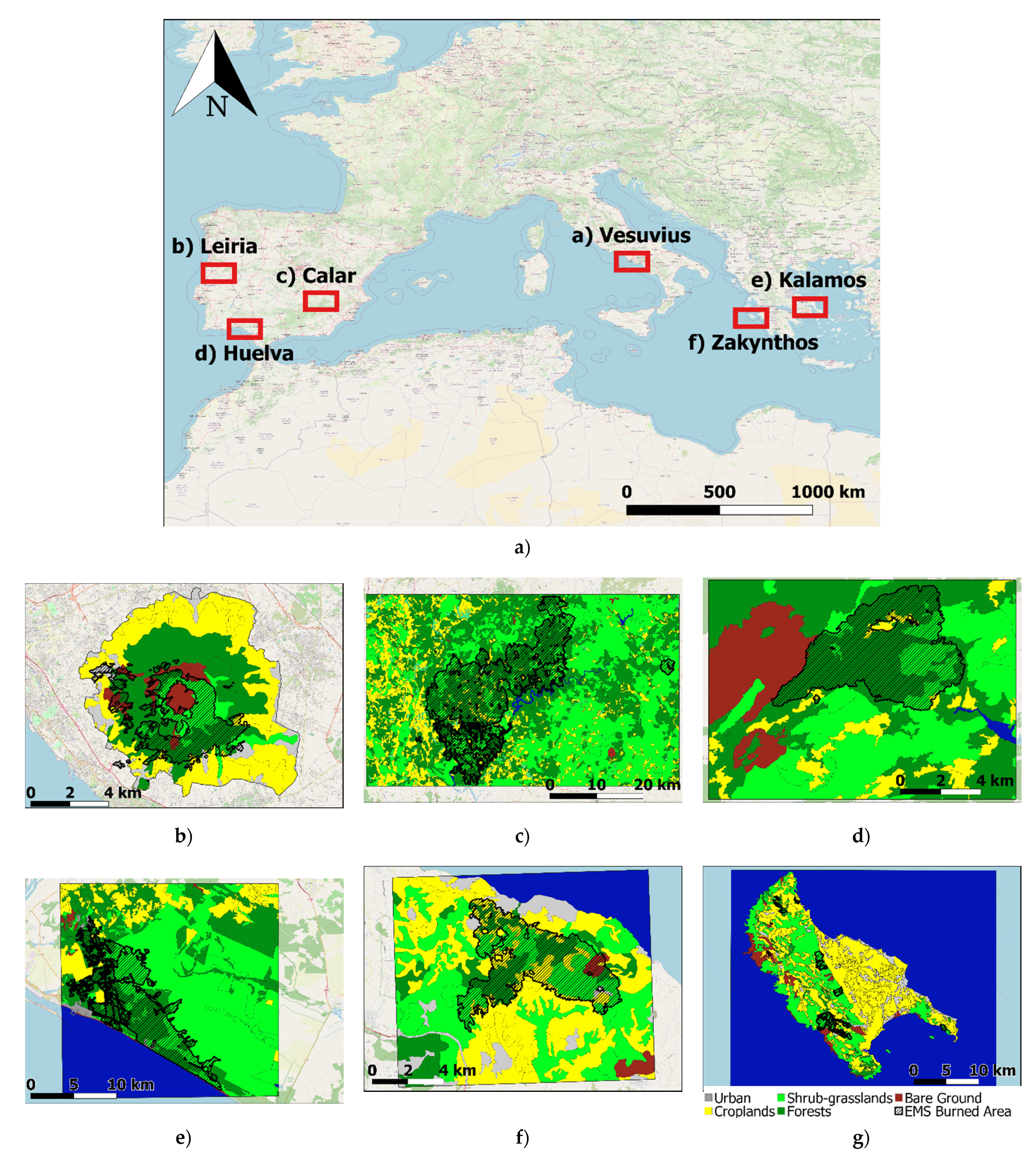
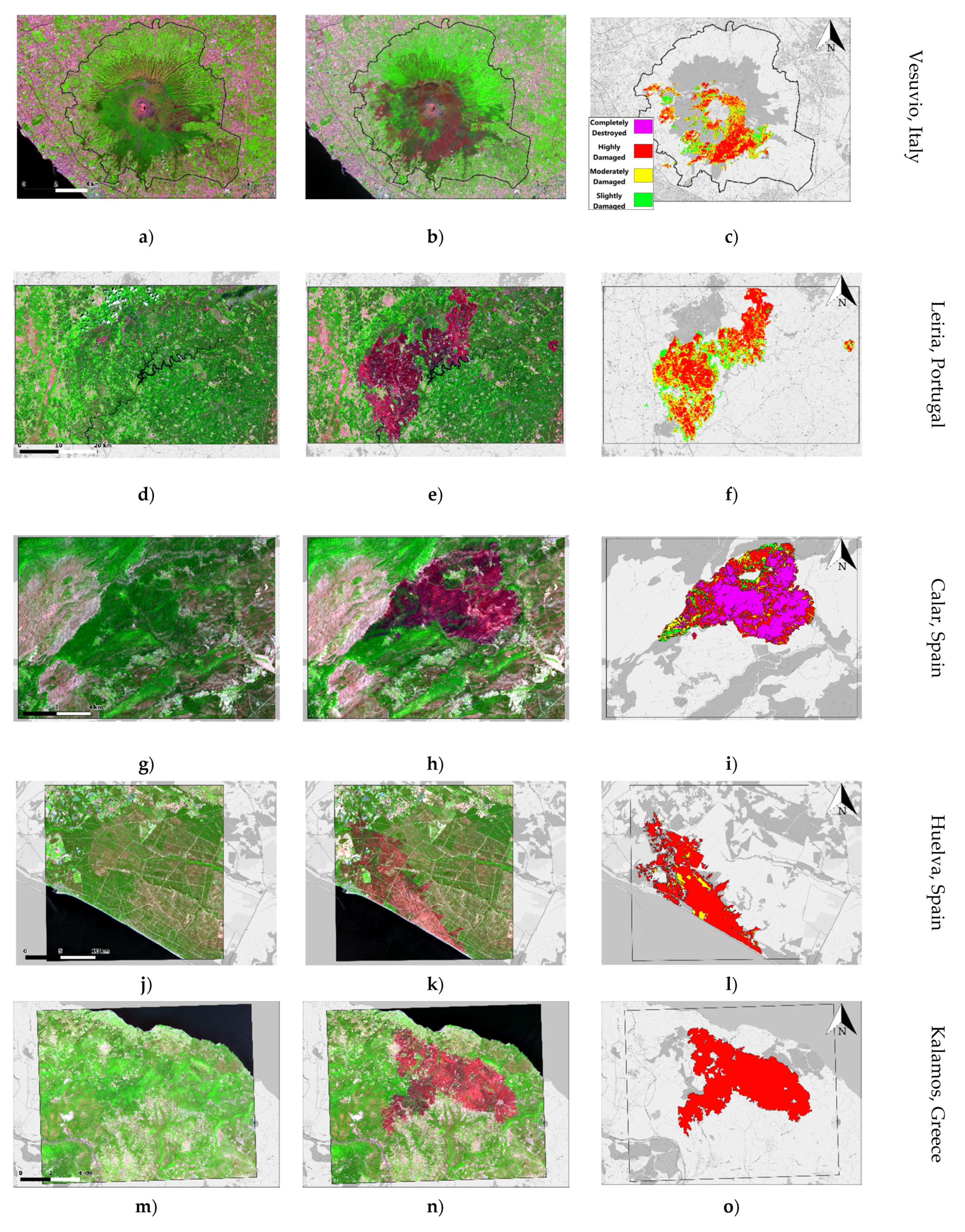
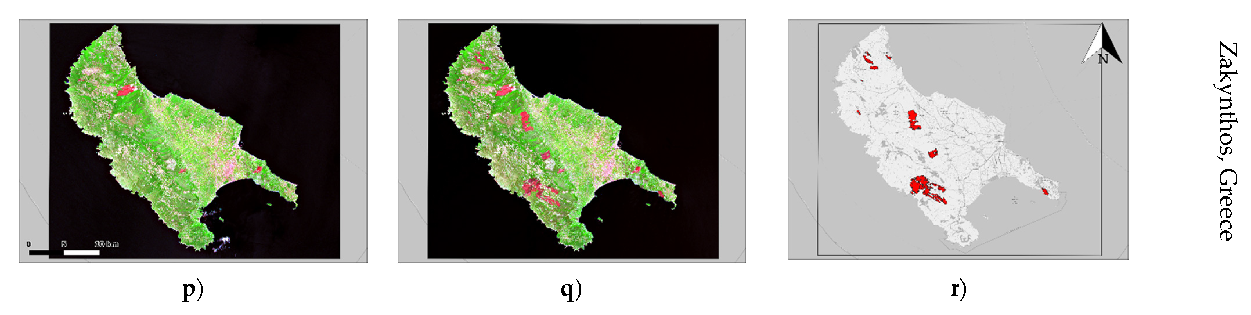
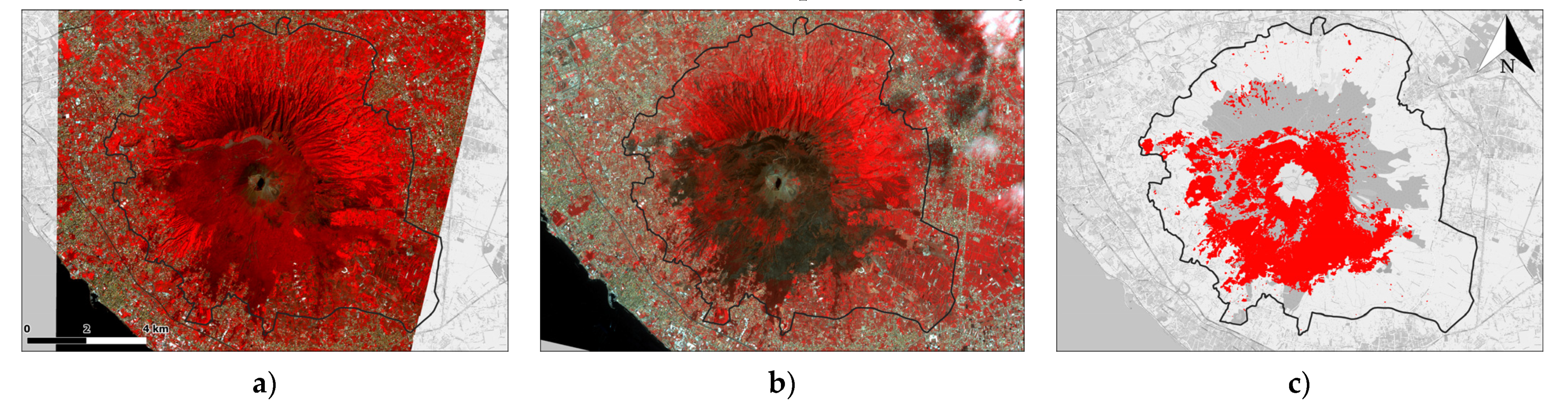
2. Study Areas and Datasets

In Southern Europe, 2017 was characterized by abnormal droughts and heatwaves [29]. Summer was the second warmest on record, with temperatures over 1.7 °C above the 1981–2010 average; the warmest being 2003 at more than 2.0 °C above average (https://climate.copernicus.eu/node/358, last access 1 May 2021). Extreme weather conditions led to severe fires affecting, in particular, Portugal, Spain, Southern France, Greece and Italy [30]. In this framework, we selected sites for algorithm training and testing that are described in the sections below.

2.1. Training and Exportability Sites

Six sites situated in Mediterranean ecosystems were selected in this work among the regions most affected by forest fires in 2017 (Figure 1). Vesuvius National Park, Italy, was used for algorithm training (development, tuning and thematic accuracy assessment) and the other five sites (Spain, Greece and Portugal) were exploited for testing algorithm exportability. The Corine Land Cover map (CLC2012, https://land.copernicus.eu/pan-european/corine-land-cover, last access 1 May 2021) was used to extract information on major land covers that are summarized in

Table 1. CLC2012 land cover classes over the entire site and within fire perimeter identified by EMS. In the last column, the proportions of fire damage levels in the burned area according to EMS fire grading products (CD = Completely Destroyed, HD = Highly Damaged, MD = Moderately Damaged and ND = Negligible to Slightly Damaged), where available.

		CLC2012 Class (%)					EMS Fire Damage
		Bare	Crops	Forest	Shrub	Urban	CD	HD	MD	ND
Vesuvius Italy	Site	6.6	38.7	36.5	10.4	7.78	0.0	12.8	3.7	2.3
	BA	3.4	4.8	47.2	34.4	10.26	0.0	68.2	19.7	12.0
Leiria Portugal	Site	0.2	15.4	43.1	40.2	1.10	0.0	8.9	5.6	2.3
	BA	-	5.6	66.7	27.5	0.17	0.0	53.0	33.1	13.8
Calar Spain	Site	13.6	8.2	61.2	17.0	-	18.9	16.5	3.6	2.0
	BA	0.3	2.4	76.4	20.9	-	46.2	40.2	8.7	4.9
Huelva Spain	Site	0.8	11.9	39.7	46.6	0.89	0.0	15.4	1.1	0.0
	BA	0.2	0.1	61.2	37.7	0.71	0.0	93.1	6.7	0.2
Zakynthos Greece	Site	5.1	52.5	32.5	3.7	6.17	-	3.2	-	-
	BA	2.3	14.6	81.8	1.3	0.02	-	100	-	-
Kalamos Greece	Site	2.0	40.6	24.2	24.7	8.36	-	20.0	-	-
	BA	3.3	25.1	33.9	36.3	1.37		100	-	-

. Most of the sites are mainly covered by natural vegetation (forest and shrub/grasslands), with the exception of Kalamos and Zakynthos where croplands are predominant, covering approximately 40% and 52%, respectively; in the Vesuvius site, forest and croplands cover similar proportions (38.7% and 36.5%). Table 1 also shows the proportion of area burned within fire polygons of the Copernicus EMS dataset among the land cover classes: in all sites, fires affected mainly forested areas, except for Kalamos, Greece, where fires affected mostly shrub/grassland (~36%).

2.2. Sentinel-2 Dataset

The remote sensing data source used for algorithm training and exportability tests was the Sentinel-2 (S2) multispectral instrument (MSI) which measures the Earth’s reflected radiance in 13 spectral bands from VIS/NIR to SWIR with a spatial resolution ranging from 10 m to 60 m (https://earth.esa.int/web/sentinel/home, last access 1 May 2021).

Over each site, pre-fire and post-fire S2 images were selected and downloaded by considering the occurrence of the major fire events, the dates of available reference datasets and the most clear sky conditions (Figure 2). Since post-fire S2 images simultaneous with reference data were desirable but hardly feasible, post-fire S2 dates were selected as close as possible to the date of reference fire perimeters (

Table 2. Pre- and post-fire S2 dates over the six sites, reference date and source for the EMS products.

Study Site	Pre-Fire S2	Post-Fire S2	EMS Date	EMS Source (https://emergency.copernicus.eu/mapping/list-of-activations-rapid, access 1 May 2021)
Vesuvius—Italy	08/04	22/07	16/07	EMSR213
Leiria—Portugal	04/06	04/07	20/06	EMSR207
Calar—Spain	15/07	04/08	04/08	EMSR216
Huelva—Spain	11/06	01/07	27/06	EMSR209
Zakynthos—Greece	25/07	03/09	18/08	EMSR224
Kalamos—Greece	28/07	17/08	18/08	EMSR224

) to minimize bias in accuracy metrics due to spectral signal changes and further burning occurring after the date of reference perimeters.

S2 images were downloaded as Level 1C from Copernicus Open Access Hub (https://scihub.copernicus.eu/, accessed 1 May 2021) since at the time of data processing no Level 2A products were available. S2 images were processed with Sen2r [31] Toolbox developed in R and released under GNU General Public License version 3 (GPL-3) and available on GitHub (https://ranghetti.github.io/sen2r, accessed 1 May 2021): Level-1C products were corrected with Sen2Cor [32] to derive bottom of atmosphere (BOA) reflectance in the VIS–NIR–SWIR wavelengths (S2 bands 2 to 12). In pre-processing steps, pixels with high and medium cloud probability were masked out while low cloud probability and cloud shadow pixels were retained to avoid discarding of burned pixels. In Sen2r, masking of cloudy pixels was done with information from the scene classification map (SCL) [33].

Output pre-processed S2 images for the selected dates were available as bottom of atmosphere (BOA) reflectance values in VIS–NIR–SWIR wavelengths (S2 bands 2 to 12) resampled to a 10 m spatial resolution with a nearest neighbor method. The temporal difference between post- and pre-fire (Δ_post-pre) reflectance was computed and, together with post-fire reflectance, band values were used as input to a separability analysis to identify features that were most suited for burned area identification. Hereafter, Δ is always meant as post-pre reflectance difference.

Training data were collected over the Vesuvius site, Italy, by photointerpretation of false color RGB (SWIR–NIR–Red) composites of S2 images (Figure 2): polygons over burned and unburned surfaces were extracted and labeled by considering as ‘burned’ only areas that were affected by fires between the two S2 dates.

2.3. Reference Fire Perimeters

Burned area maps output from the proposed algorithm were validated by comparison with fire reference perimeters obtained from independent source data. In all sites, major fires occurred during the 2017 summer season, affecting, to a large extent, ecosystems, houses and people, so the Copernicus Emergency Management Service (EMS) was activated. EMS consists of the on-demand and fast provision (hours–days) of geospatial information in support of emergency management activities and derived from processing and analysis of satellite imagery acquired immediately after natural or human-made disasters such as floods, droughts and forest fires. EMS products are delivered as ready-to-print maps and geographic datasets (vector package). Two types of geo-products are delivered: fire delineation (fire perimeter) and fire damage grading (burn severity) derived from very high-resolution multispectral images. Fire damage grading is provided in four classes: “Completely Destroyed”, “Highly Damaged”, “Moderately Damaged” and “Negligible to Slightly Damaged”. Quality checks are performed by the European Commission Joint Research Centre (EC JRC) to assure fast delivery of high-quality products. Further validation activities can be carried out by the EC JRC if triggered by the European Commission and/or suggested by authorized users; further information can be found in the ‘Online Manual for Rapid Mapping Products’ (https://emergency.copernicus.eu/mapping/ems/online-manual-rapid-mapping-products, last access 1 May 2021).

Table 2 summarizes the reference dates of the EMS delineation and grading map source (where available). EMS delineation maps were used as source datasets for fire reference perimeters for all sites, except Vesuvius where EMS maps depicted the status of the surface on 16 July 2017. Yet, ongoing fires made the time gap between the EMS and S2 post-fire date (22 July 2019) critical for the comparison and for the estimation of reliable accuracy metrics (Appendix A, Figure A1). Hence, to generate a reference dataset suitable for validation, very high-resolution (VHR) PlanetScope images [34] were used.

PlanetScope is a constellation composed of more than 120 optical CubeSat 3U satellites carrying a multi-spectral sensor with four bands: three in the visible wavelengths (b1: 455–515 nm; b2: 500–590 nm; b3: 590–670 nm) and one in the NIR wavelengths (b4: 780–860 nm) (https://earth.esa.int/web/guest/missions/3rd-party-missions/current-missions/planetscope, accessed 1 May 2021). PlanetScope has a swath of about 25 Km and a spatial resolution of 3 m for all bands [35]. Imagery is captured as a continuous strip of single frame images known as ‘scenes’.

Pre- and post-fire PlanetScope images (22 April and 22 July 2017) were downloaded and classified with a supervised random forest (RF) algorithm to extract fire perimeters (Figure 3). The RF classifier is a machine learning algorithm that is largely used in remote sensing [36,37]. It builds an ensemble of decision trees (CART) and merges them together to yield a more accurate and stable prediction than any single tree alone [38]. The map generated at high resolution (~3 m) can be considered spatial explicit ground truth information for the assessment of S2 products (namely 10 m resolution).

3. Methods

The proposed algorithm relies on a multi-criteria approximate reasoning approach that aggregates information brought by multiple features into synthetic global degrees of evidence of burn. Each input feature could be used as source for deriving evidence of burn conditions (partial evidence) but aggregation reinforces evidence by exploiting the convergence of partial evidence from multiple possibly redundant sources and by compensating the inconsistency/conflict of evidence from multiple possibly complementary sources. This step allows strengthening of the likelihood of the presence of burn and reduces confusion between burned areas and surfaces with similar spectral characteristics [26]. Aggregation was carried out with ordered weighted averaging operators (OWAs): a parameterized family of soft-mean-like aggregation operators. Different operators were used to represent attitudes ranging between pessimistic (the maximum extent of the phenomenon to minimize the chance of underestimating: modeling a compensative aggregation to integrate complementarities of multiple criteria) and optimistic (minimize the chance of overestimating: modeling a concurrent aggregation to integrate mutual reinforcement of multiple criteria). Layers of global evidence derived with different OWAs were input to a region growing (RG) algorithm. The approach was applied independently to each pixel of the input RS images as follows:

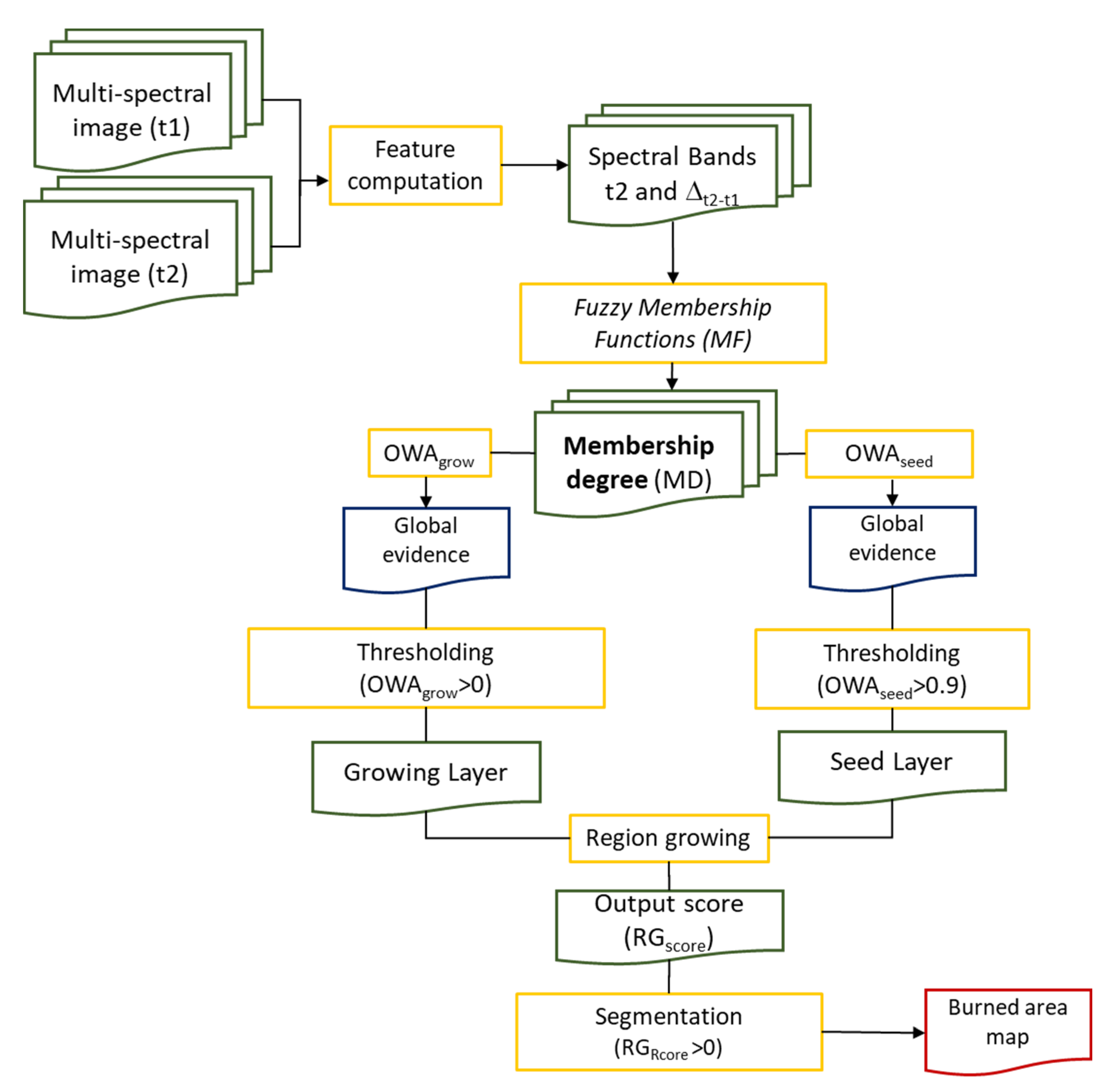
• Selection of the input features;
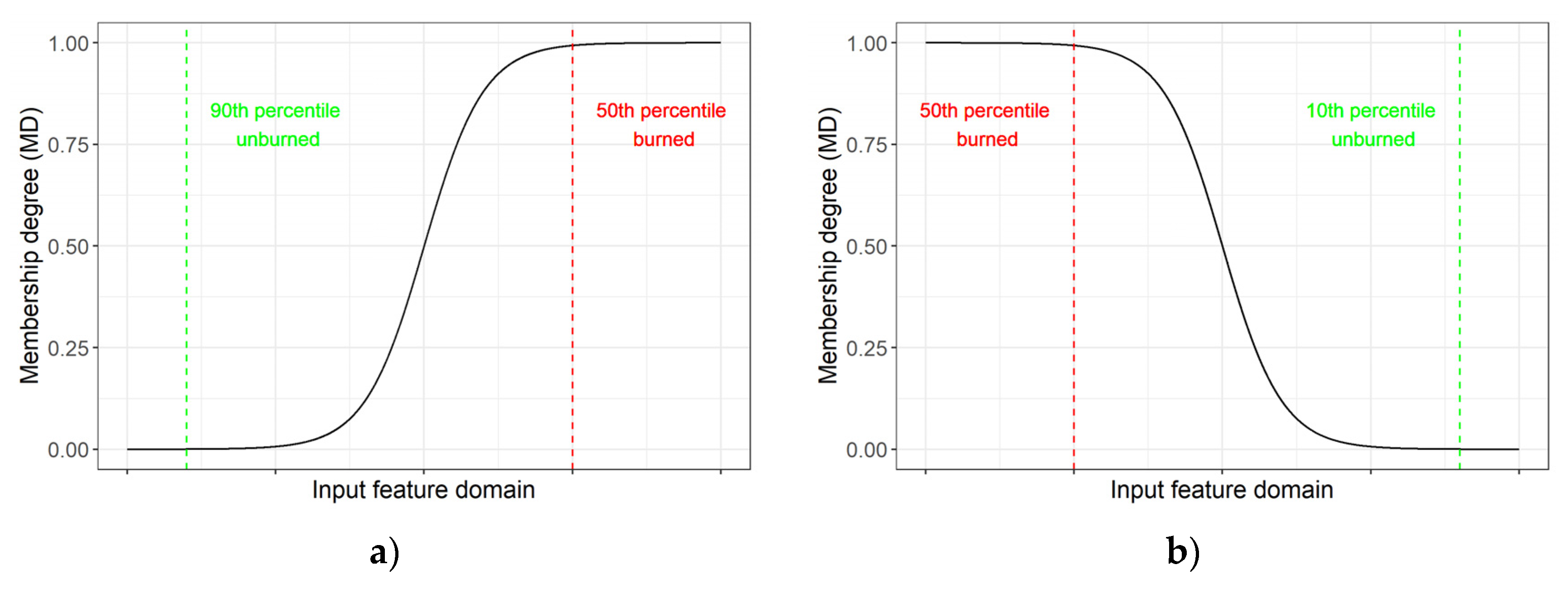
• Definition of the soft constraints (membership function, MF) for each input feature from training data and application to derive partial evidence of burn (MD);
• Selection of OWAs, according to their semantic, for the soft integration;
• Computation of the global degree of evidence of burn for generating seed and growing layers;
• Implementation of the RG algorithm;
• Segmentation of the RG output score to derive burned area maps.

The algorithm was applied to vegetated areas, while not burnable (bare soil and urban classes) and agricultural areas were masked out based on the CLC2012 land cover map. Output burned area maps were compared to reference datasets for estimating accuracy metrics. Steps (1) to (6) were applied over the training site (Vesuvius, Italy) for the selection of the best input features, the definition of the membership functions and the customization of the RG algorithm. Exportability was tested over the other sites by applying steps (4) to (6) to assess the algorithm’s performance over geographic locations with different environmental conditions compared to those of the training site.

3.1. Separability Analysis

A separability analysis was preliminarily carried out over the Vesuvius training site for selecting the most suitable bands for the discrimination of burned and unburned surfaces. Separability metric M (1) was computed from frequency distributions of training pixels [39].

$$M=\left|\frac{{\mathsf{\mu }}_{\mathrm{u}}-{\mathsf{\mu }}_{\mathrm{b}}}{{\mathsf{\sigma }}_{\mathrm{u}}+{\mathsf{\sigma }}_{\mathrm{b}}}\right|$$

(1)

where μ_u, μ_b are mean values and σ_u, σ_b are standard deviation values of the unburned (u) and burned (b) classes in the training data. Spectral bands with M > 1 were selected as input features for the computation of the partial evidence of burn.

3.2. Definition of the Membership Functions

Membership functions (MFs) are soft constraints that can be defined with different approaches according to the available expertise and training data [40]. Here, soft constraints were defined from training data over the Vesuvius site for each input feature identified by the separability analysis. MFs are sigmoid Functions (2) used to convert a pixel’s values of the input feature into degrees of membership to the burned class (membership degree, MD), i.e., the partial evidence of burn that is a score in the range [0, 1]. The extremes of the sigmoid-shaped MFs were defined based on percentiles of the unburned and burned histogram distributions, respectively [19].

$$f\left(x\right)=\frac{L}{1+e^{-k\left(x-x0\right)}}$$

(2)

where L is the upper limit of the function, in this case L→1 to quantify the maximum degree of membership, k is the curve’s slope and x0 is the inflection point. The two parameters k and x0 are estimated by using percentiles.

Based on Roteta et al. (2019) [19], we selected a different shape for the sigmoid functions depending on the spectral characteristics of burned areas in the specific input feature: a z-shaped function or s-shaped function. The upper limit of the function f(x)→1 represents the greatest partial evidence of burn defined by a pixel’s values of the input features below and above the 50th percentile of the frequency distribution function of the burned training pixels for z-shaped and s-shaped functions, respectively (Figure 4). On the opposite side, f(x)→0 (no partial evidence of burn) and it is given by the 10th and 90th percentile of the frequency distribution function of the unburned training pixels for the z-shaped and s-shaped function, respectively. Training pixels for burned and unburned categories, extracted over the Vesuvius training site, were used to estimate k and x0 parameters: a z-shaped function was used when fire occurrence led to a decrease in the pixel’s value in a given input feature, for example, in the NIR S2 reflectance band. On the contrary, an s-shaped function represents the case when per-pixel input feature value increases over a burned area.

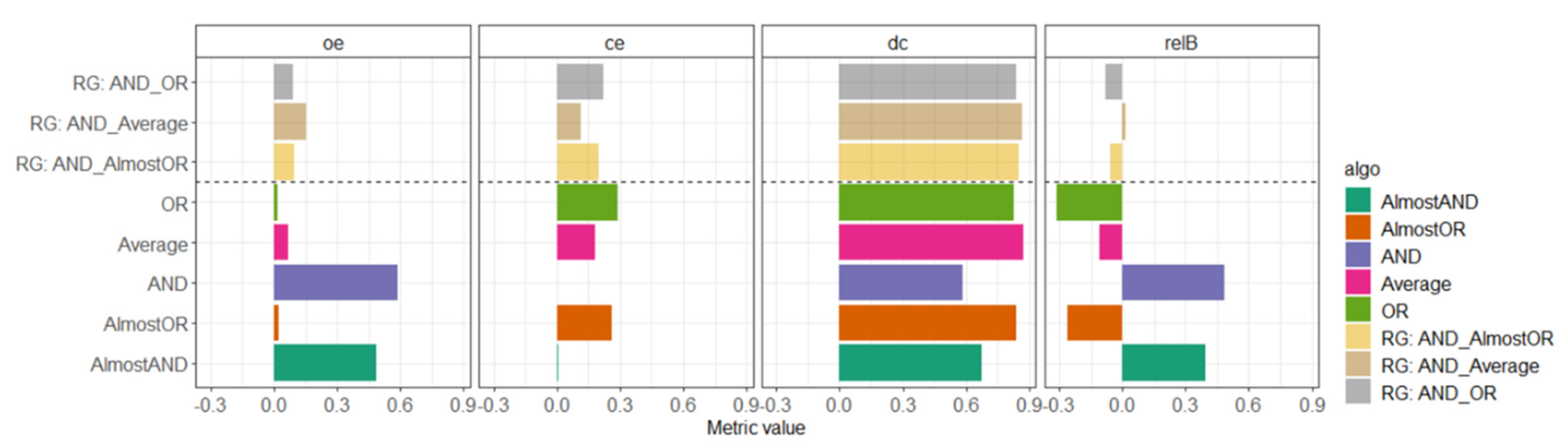
3.3. OWA Operators for Computing Global Evidence

Layers of partial evidence were integrated to derive global scores of burn evidence with ordered weighted averaging (OWA) operators [28]. An OWA of dimension N (OWA: [0, 1]^N → [0, 1]), where N is the number of input values [d₁, …, d_N] to aggregate, has a weighting vector W = [w₁,…,w_N], with ∑_i=1,...,N w_i = 1, so that it computes an aggregated output value a ∈ [0, 1] by applying the following formula [41]:

$$a=OWA\left(\left[d_1, \dots ,d_N\right]\right)={\displaystyle \sum }_{i=1}^N{w}_i\ast g_i$$

(3)

where g_i is the i^th largest value among the input d₁,…,d_N.

Input values d₁,…,d_N, are rearranged from the highest to the smallest; reordering is a key element of OWA operators, meaning that a specific weight w_i is not univocally associated to the specific i^th input but rather it is associated with the i^th position of the reordered inputs [28]. Since, in our case, OWAs aggregated the MDs expressing partial evidence of burn provided by single features, in each pixel, a different reordering of the MDs may have occurred so different features contributed to determining the aggregated value.

Different operators were tested to represent decision attitudes between pessimistic (the maximum extent of the phenomenon to minimize the chance of underestimating) and optimistic (to minimize the chance of overestimating). For example, a weighting vector W of the OWA operator with the last weight w_N = 1 considers only the contribution of the smallest input value, i.e., the minimum partial evidence degree after reordering; hence, it implements an optimistic attitude by computing the minimum total burned area (AND aggregation). Conversely, by setting the first weight w₁ = 1, the maximum partial evidence will determine the largest burned area, thus modeling the pessimistic case (OR aggregation). Intermediate cases, in which all or most components of W are not null, model soft integrations.

In this work, we compare the results obtained by applying five different OWA operators with the following weighting vectors:

$$\begin{array}{cc}{W}_{AND}=\left[0,\dots , 0, 1\right]& \mathrm{thus} OW{A}_{AND}\left(\left[d_1, \dots , d_N\right]\right)=\min {\left\{d_1, \dots , d_N\right\}}_{ }\\ W_{OR}=\left[1,\dots , 0, 0\right]& \mathrm{thus} OW{A}_{OR}\left(\left[d_1, \dots , d_N\right]\right)=\max {\left\{d_1, \dots , d_N\right\}}_{ }\\ W_{AlmostAND}={\left[0, \dots , 0.5, 0.5\right]}_{ }& \mathrm{thus} OW{A}_{AlmostAND}\left(\left[d_1, \dots , d_N\right]\right)=\frac{1}{2}\min \left\{d_1, \dots , d_N\right\}+\frac{1}{2}\min \{\left\{d_1, \dots , d_N\right\}-\left\{\min \left\{d_1, \dots , d_N\right\}\right\}\\ W_{Aaverage}={\left[\raisebox{1ex}{$1$}\!\left/ \!\raisebox{-1ex}{$N$}\right.,\dots , \raisebox{1ex}{$1$}\!\left/ \!\raisebox{-1ex}{$N$}\right.\right]}_{ }& \mathrm{thus} OW{A}_{Average}\left(\left[d_1, \dots , d_N\right]\right)=\frac{1}{N} \sum _{j=1}^N{d}_j \\ W_{AlmostOR}={\left[0.5, 0.5, 0, \dots , 0\right]}_{ }& \mathrm{thus} OW{A}_{AlmostOR}\left(\left[d_1, \dots , d_N\right]\right)=\frac{1}{2}\max \left\{d_1, \dots , d_N\right\}+\frac{1}{2}\max \{\left\{d_1, \dots , d_N\right\}-\left\{\max \left\{d_1, \dots , d_N\right\}\right\}\end{array}$$

The output of an OWA operator applied to all pixels in an image is a gray-level image whose pixels take values in [0, 1], where each pixel’s value is the global evidence of burn: in Figure 5, this step performs the dimension reduction from N input features (MD scores for each pixel) to 1 (synthetic score). OWA layers are then input to the region growing algorithm.

3.4. Region Growing

The RG algorithm, implemented in Harris IDL language (https://www.l3harrisgeospatial.com/docs/region_grow.html, last access 1 May 2021), needs as input a seed layer (OWA_seed) and a growing layer (OWA_grow) and two conditions (thresholds) on OWA_seed and OWA_grow to identify seed pixels and to delimit maximum growing boundaries. Seed and growing layers are selected among the layers of global evidence generated with distinct OWAs: one concurrent for the seed layer whose segmentation is set to minimize commission errors, and one compensative for the grow layer, whose segmentation is set to minimize omission errors by expanding seeds. Hence, seeds are extracted from the most restrictive OWA_AND while growing boundaries are derived from less restrictive OWAs (OWA_OR, OWA_Average, OWA_AlmostOR). While the requirement on the seed layer is very high, the strategy for identifying candidate boundaries (i.e., the limits for the region growing) can be looser, thus allowing the algorithm to also expand over pixels with low burn signal but connected to more reliable pixels, i.e., the seeds (e.g., partially burned pixels along the perimeter of the burned patches). The RG algorithm is an iterative algorithm that at each iteration expands the seed pixels: starting from initial seeds (pixel with OWA_AND above a given threshold), it searches the 8-neighbor connected pixels and it includes in the seed layer only those pixels with OWA_grow > 0. These expanded pixels update the seeds for the next iteration cycle. The iteration ends when boundaries of maximum growth is reached in the OWA_grow layer. The output layer is a gray-level image (RG_score ∈ [0, 1]) whose values can be further segmented to generate the maps of burned/unburned areas (binary maps).

Preliminary analysis carried out over the training site allowed the definition of the implementation conditions of the RG algorithm: thresholds for seed and growing layers as well as a threshold for the segmentation of the RG_score. The criterion set for seed selection is OWA_AND > 0.9; no change in burned area mapping accuracy was observed for different thresholds applied to OWA_AND due to its frequency distribution with a bimodal shape centered over extreme values 0 (no evidence of burn) and 1 (full membership to the burned class, greatest evidence of burn) (not shown). For the growing layer, different conditions on the value of OWA_grow were analyzed to identify the maximum growing boundary (S.2, S.3), showing that the highest accuracy is achieved when all pixels with not null evidence are retained (OWA_grow > 0). Finally, in the segmentation step on RG_score, the analysis of variable thresholds showed that RG_score > 0 provides the greatest accuracy (S.2, S.3). As a result of these preliminary analyses, Figure 5 shows the flowchart of the algorithm proposed in this work.

3.5. Validation

The accuracy of the output burned area maps was estimated by comparison with reference fire perimeters (i.e., fire polygons from RF classification of PlanetScope images for the Vesuvius site and Copernicus EMS fire delineation layers). Over the Vesuvius site, accuracy assessment was part of the training phase for the definition of the best implementation criteria of the algorithm. Over the other sites, accuracy assessment of the burned area maps obtained by applying the algorithm in its final form contributed to the evaluation of the exportability. In both cases, validation was carried out by estimating metrics from the confusion matrix (commission error, omission error, Dice coefficient and relative bias) [42]. In order to build the confusion matrix, score map output from the RG algorithm was segmented to extract burned/unburned areas in a binary form (RG_score > 0, S.3). In the Results section, accuracy metrics are presented and discussed as a function of the OWA_grow layer.

4. Results

4.1. Separability and Membership Functions

Results of the separability analysis depict the distance between burned and unburned classes, as observed in the post-fire and Δ_post-pre S2 reflectance bands for the Vesuvius site (

Table 3. Separability metric M measuring the distance between burned and unburned surface spectral signal in the post-fire and post-pre fire reflectance of the S2 bands. Bold numbers highlight values M > 1 of the selected features.

S2 Band	M Post fFire	M ΔPost Fire-Pre Fire
Green (b3)	0.577	0.027
Red (b4)	0.321	0.454
RE1 (b5)	0.879	0.214
RE2 (b6)	2.091	1.571
RE3 (b7)	1.917	1.561
NIR (b8)	1.812	1.530
SWIR1 (b11)	0.873	0.099
SWIR2 (b12)	0.029	1.100

); M > 1 highlights a good separability that is, in this case, achieved by S2 post-fire red–edge (RE2, RE3) and NIR bands and their temporal difference (Δ_post-pre). S2 SWIR2 post-fire reflectance provides very poor separability (M < 0.1) that increases when temporal difference (Δ_SWIR2) is computed, suggesting that the difference with respect to pre-fire unburned conditions enhances separability; the opposite occurs for the S2 SWIR1 band. Reflectance of burned surfaces is the result of a mixture of bare soil, unburned vegetation and combustion products (ash, charcoal) that are present on the surface after a fire. The combustion of vegetation significantly influences the post-fire spectral signature by generally decreasing reflectance (μ_b), thus enhancing the difference with respect to unburned conditions (μ_u), especially in the NIR wavelengths. For longer wavelength bands (i.e., SWIR2), the spectral reflectance of dry unburned vegetation (green vegetation proportion absorbing radiation due to water content) and burned surfaces could be equally low, thus reducing separability (lower M value). The separability power of SWIR wavebands in the temporal change detection algorithm has also been widely exploited as an indicator of burn severity although the sensitivity of these bands has been found to vary geographically [43]. Red–edge bands show good separability for wavelengths longer than 740 nm (RE2 and RE3), and are certainly of great interest, although these bands are not present on all space-borne sensors and they are mainly selected for vegetation chlorophyll content estimation and monitoring [44].

Based on these results, the following seven input layers were selected as features for the implementation of the algorithm (Figure 5): post-fire NIR, post-fire RE2 and RE3 and temporal difference (Δ_post-pre) of the same three bands and additionally of SWIR2. From the same training dataset, statistics for burned and unburned surfaces were computed for the estimation of the k and x0 parameters of the membership functions (

Table 4. Percentiles of the frequency distribution functions extracted from the training pixels of the study area and used for defining MFs.

S2 Band	Burned			Unburned			MF Parameters
	10%	50%	90%	10%	50%	90%	k	x0
PostRE2	0.058	0.074	0.102	0.147	0.220	0.286	−125.89	0.111
PostRE3	0.061	0.077	0.112	0.156	0.249	0.339	−115.77	0.116
PostNIR	0.054	0.073	0.115	0.147	0.264	0.370	−123.66	0.109
ΔRE2	−0.126	−0.098	−0.063	−0.021	0.012	0.088	−120.29	−0.06
ΔRE3	−0.158	−0.124	−0.075	−0.026	0.012	0.108	−93.721	−0.075
ΔNIR	−0.180	−0.139	−0.085	−0.034	0.011	0.111	−87.14	−0.086
ΔSWIR2	0.025	0.063	0.114	−0.030	0.0084	0.024	236.98	0.044

). MFs map the input feature’s values into the [0, 1] domain where values closer to 1 (0) represent the greatest (lowest) likelihood of being burned. Among the selected features, only Δ_SWIR2 was properly described by an s-shaped function since, according the training dataset, over burned areas, Δ_SWIR2 > 0.

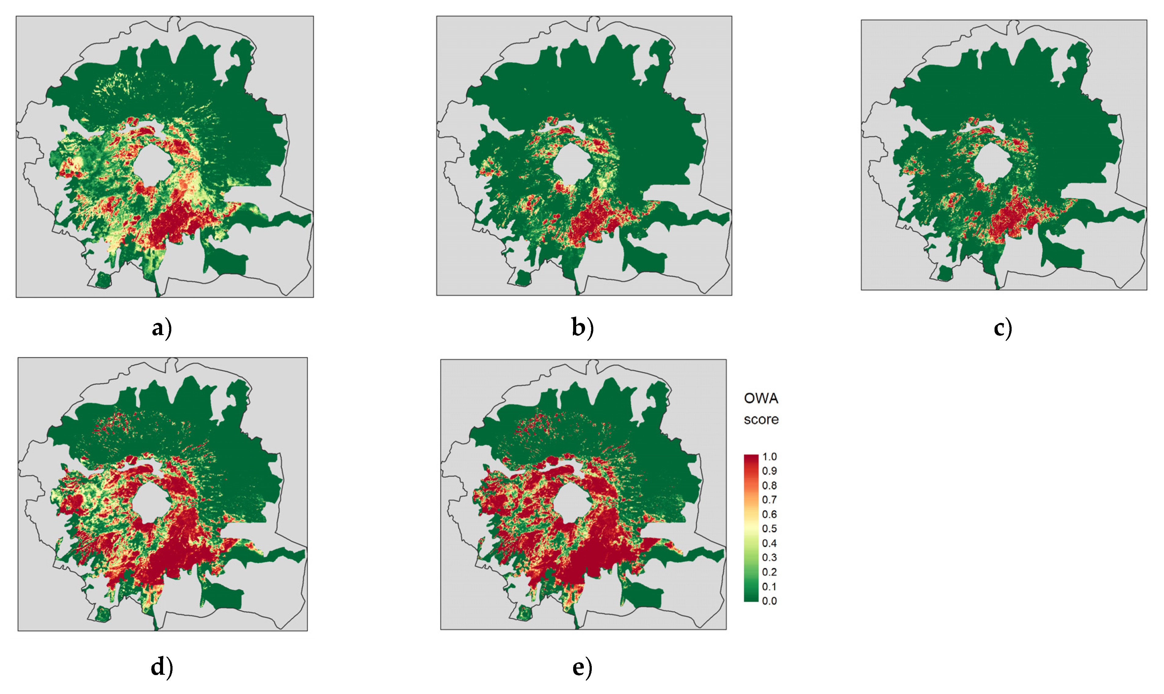
4.2. Partial and Global Evidence of Burn

MFs are applied to the input features to derive maps of partial evidence of burn (MD = membership degree score). Figure 6 shows the partial evidence of burn for the training site: greater MD values represent higher likelihood of burn (from blue to yellow in the figure) and the frequency distribution of pixel values varies with the input feature according to its sensitivity in detecting different burned conditions. Areas located in the southernmost regions of the park that were severely affected by fires during summer 2017 are consistently identified by all features with the greatest values (yellow regions). Differences in the partial evidence of burn brought by single features are mainly observed in the northern regions; in fact, each feature is sensitive to different characteristics of the burned surfaces and/or different degrees of burn. In the figure, non-forested areas within the border of the national park are masked out and shown in gray.

Global evidence of burn is computed with OWA operators integrating partial evidence, as shown in Figure 7 for the Vesuvius training site. OWA score ranges within [0, 1], with the greatest values showing pixels with the highest likelihood of being burned according to convergent evidence of burn from the input layers. All OWA maps highlight regions of the Vesuvius site most affected by fires in the southernmost areas, where all input layers agree on identifying higher partial evidence of burn. The ‘concurrent–strict’ to ‘complementary–relaxed’ integration conditions implemented by the different OWAs supported the choice of seed and growing layers for the RG algorithm: we selected OWA_AND as the seed layer combined with average and OR-like OWAs as the growing layer (OWA_Average, OWA_AlmostOR and OWA_OR). Once seed pixels were selected (OWA_AND > 0.9), the RG algorithm expanded the initial selection in an iterative way over the OWA_grow layer in order to also capture pixels with lower values of global evidence (less likely to be burned).

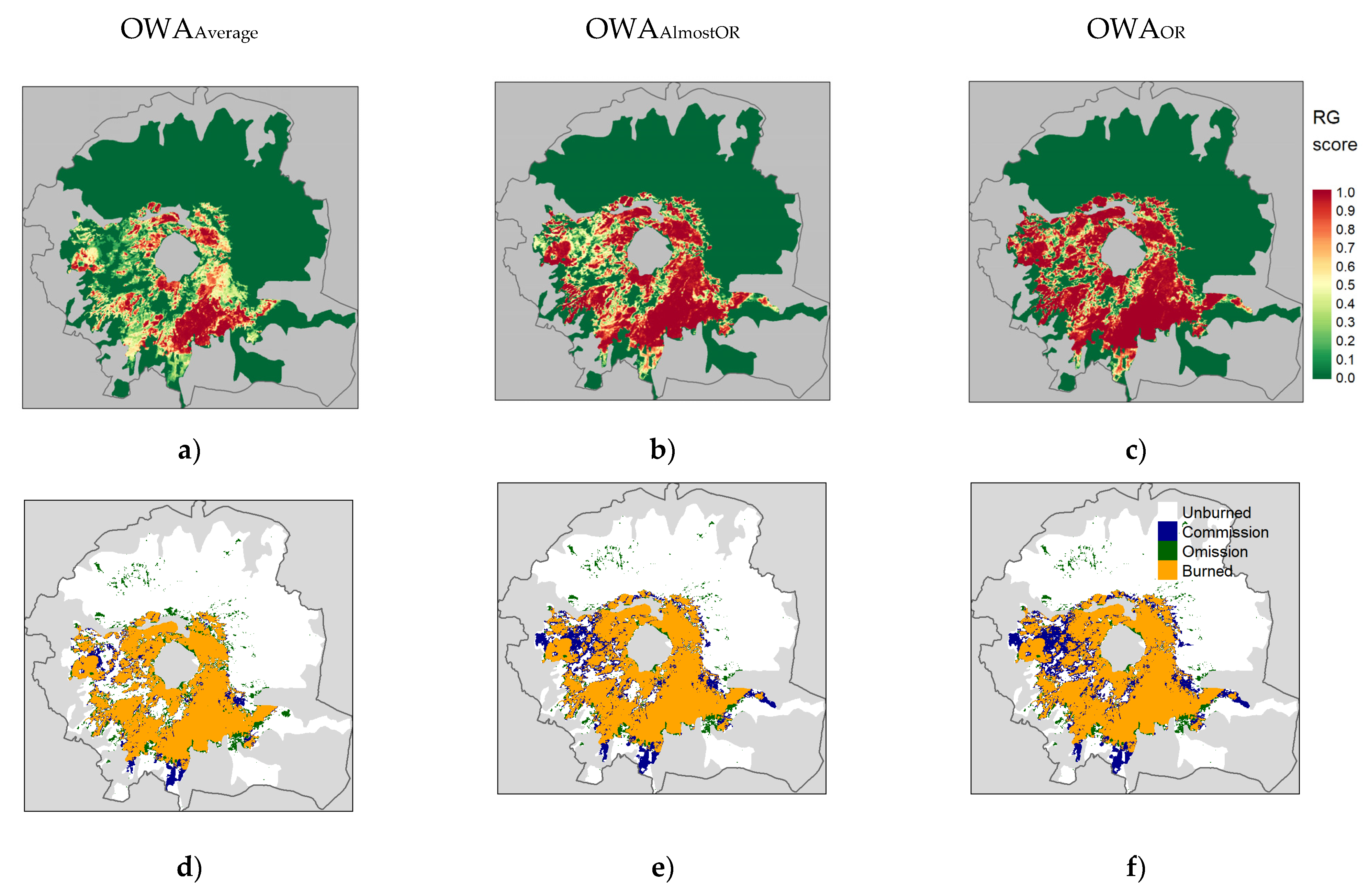
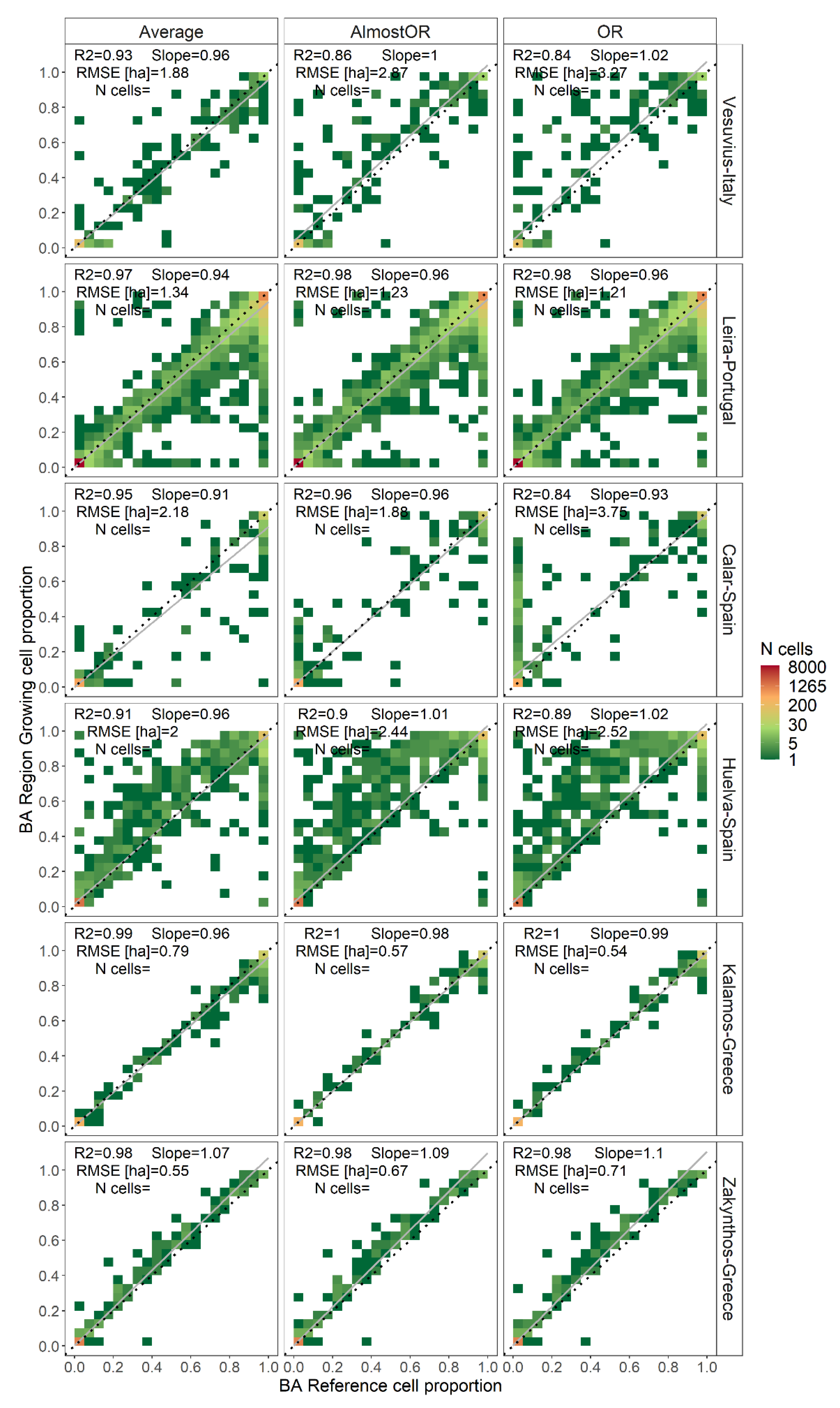
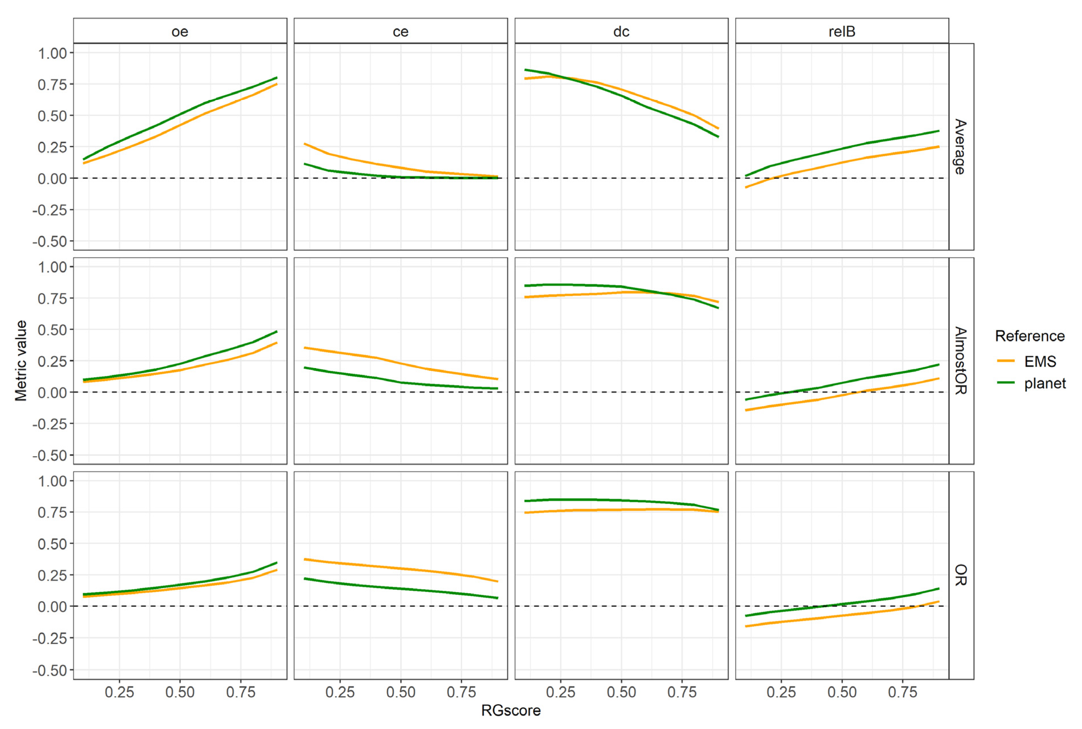
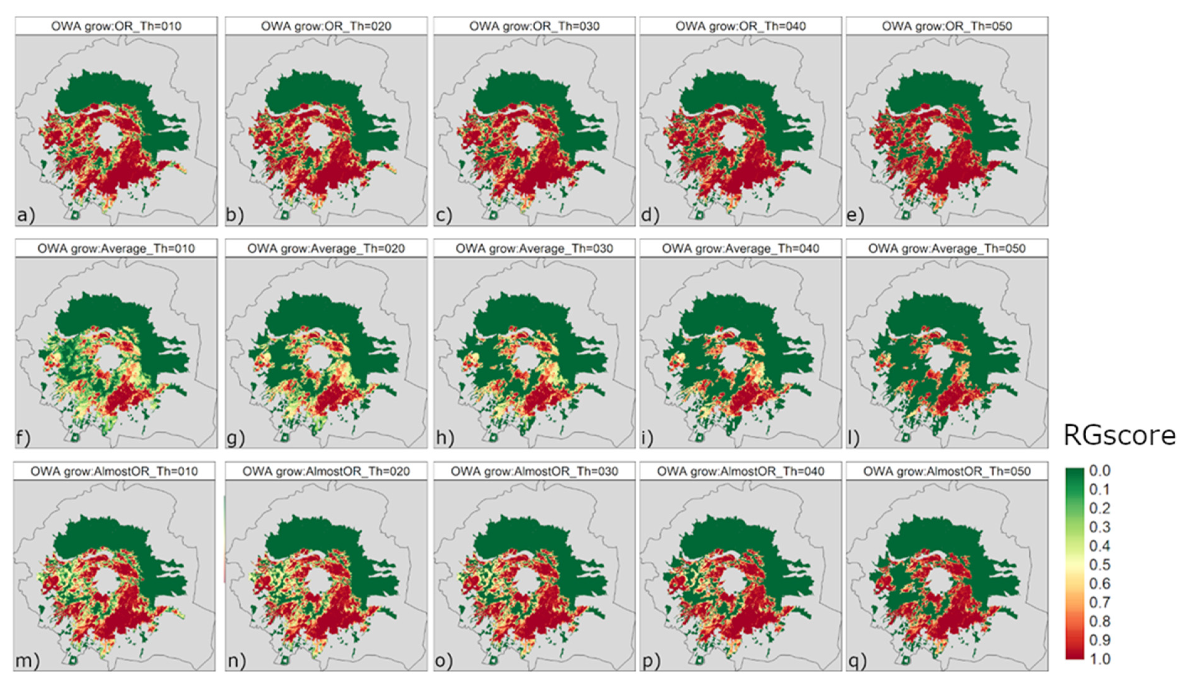
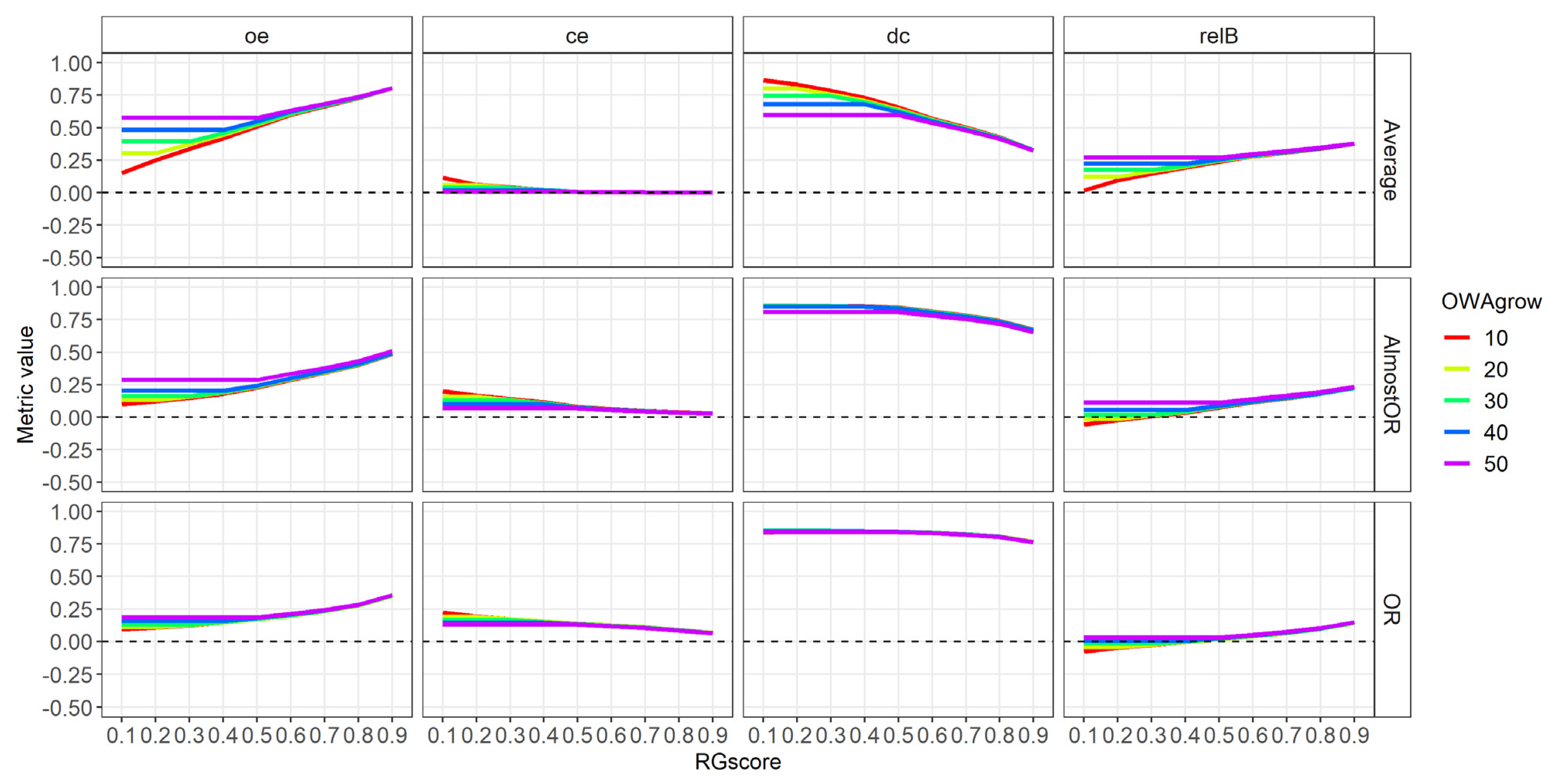
4.3. RG Burn Score and Validation

Figure 8 shows the RG_score (top row) and agreement (bottom row) maps that depict the spatial distribution of agreement between the two-class algorithm’s output and the reference datasets: full agreement over burned (orange) and unburned classes (white) as well as errors of omission (green) and commission (blue).

In the agreement maps, omission errors in the northern slopes of the volcano are mainly produced by the lack of seed pixels in the OWA_seed layer (Figure 7a), likely due to low-intensity and/or below-canopy fires; these regions are common to all output RG_score maps since the omission error descends from the seed layer rather than the growing layer. Commission errors are larger in the maps produced with OWA_AlmostOR and OWA_OR that implement ‘complementary–relaxed’ aggregation. Accuracy metrics quantifying the errors depicted in Figure 8 are summarized in

Table 5. Accuracy metrics (oe = omission error, ce = commission error, dc = Dice coefficient, relB = relative bias) over the Vesuvius site for the three (OWA_Average, OWA_AlmostOR and OWA_OR) growing layers. The total amount of burned area from the algorithm (Tot BA RG) and the reference (Tot BA REF) are also given.

OWAgrow	oe	ce	dc	RelB (%)	Tot BA RG (ha)	Tot BA REF (ha)
Average	0.15	0.12	0.87	+1.82	1676.39	1744.07
AlmostOR	0.10	0.20	0.85	−5.81	1959.69
OR	0.09	0.22	0.84	−7.70	2029.95

together with total estimated hectares of area burned (Tot BA).

Results show that omission error is below 0.15 while commission error is in the range [0.12–0.22]. Commission is greater than omission for OWA_AlmostOR and OWA_OR growing layers, while OWA_Average leads to the greatest underestimation. Over the training site, total estimated burned area from the RG algorithm ranges between 1676.39 ha and 2029.95 ha, while the reference dataset provides 1744.07 ha of area burned. Saulino et al. (2020) [45] estimated that the area burnt by summer wildfires in 2017 in Vesuvius National Park amounted to 3350.23 ha, although this estimate covers the entire summer season by including fires that occurred later than the S2 post-fire date, 22 July.

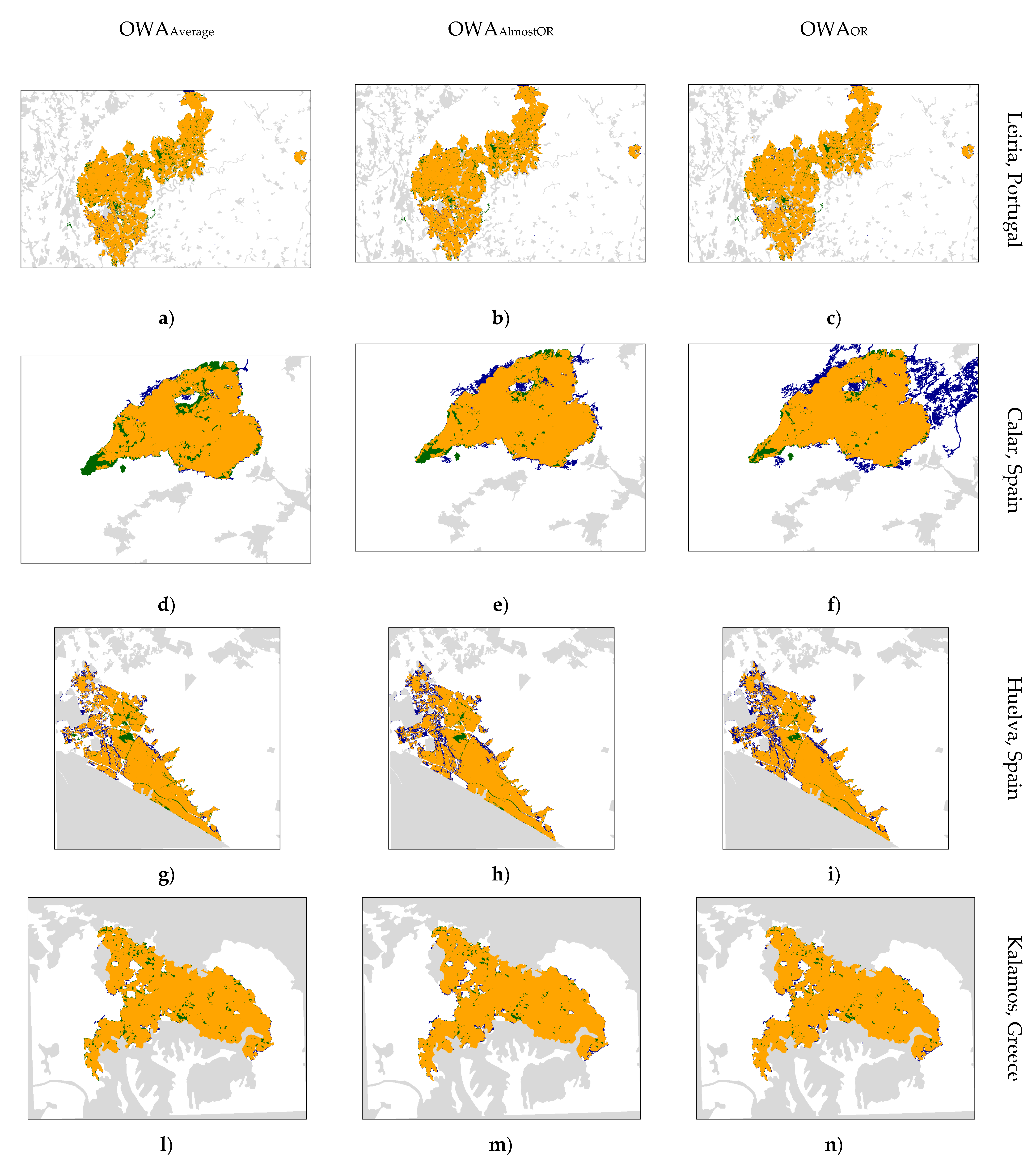
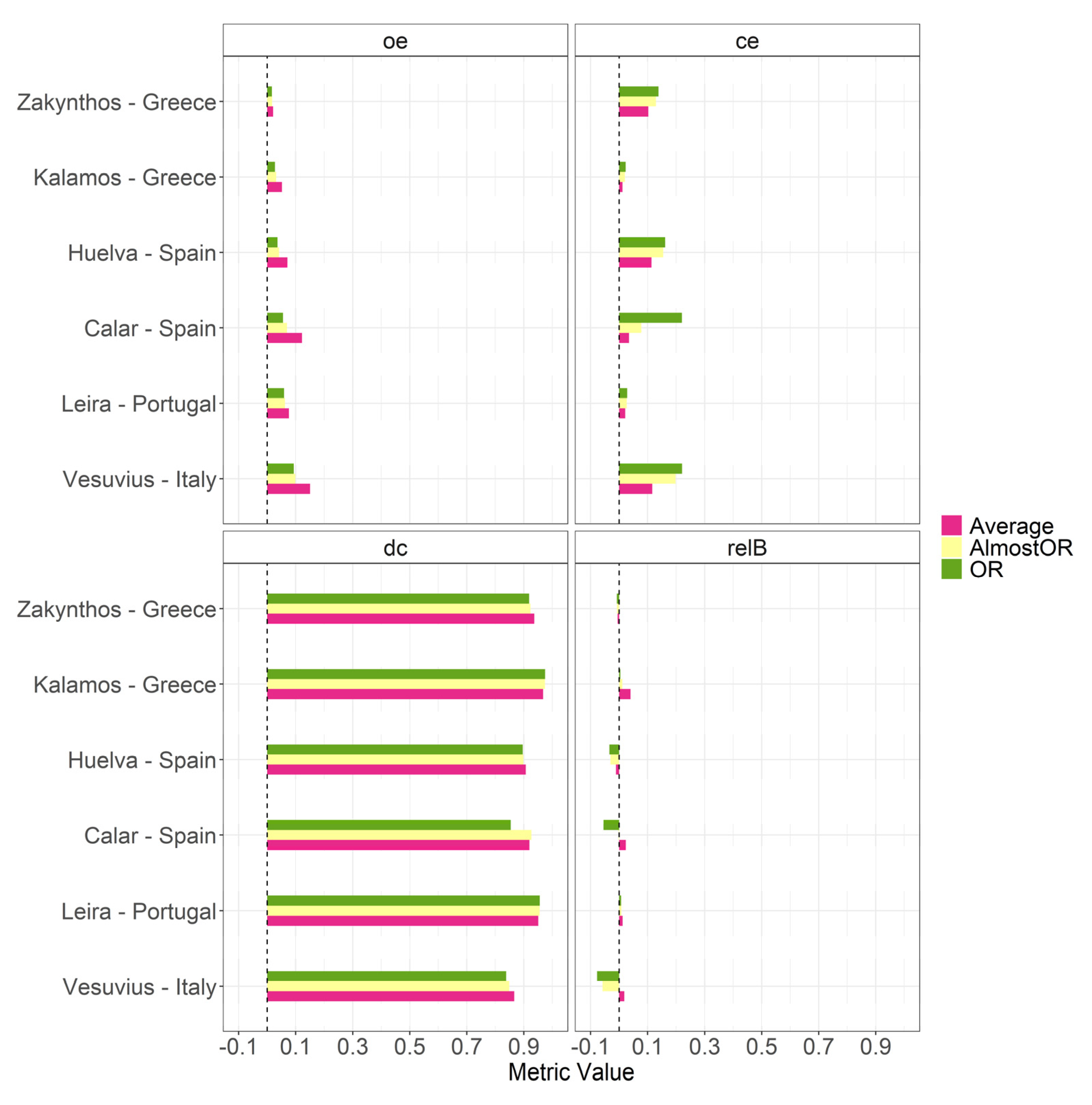
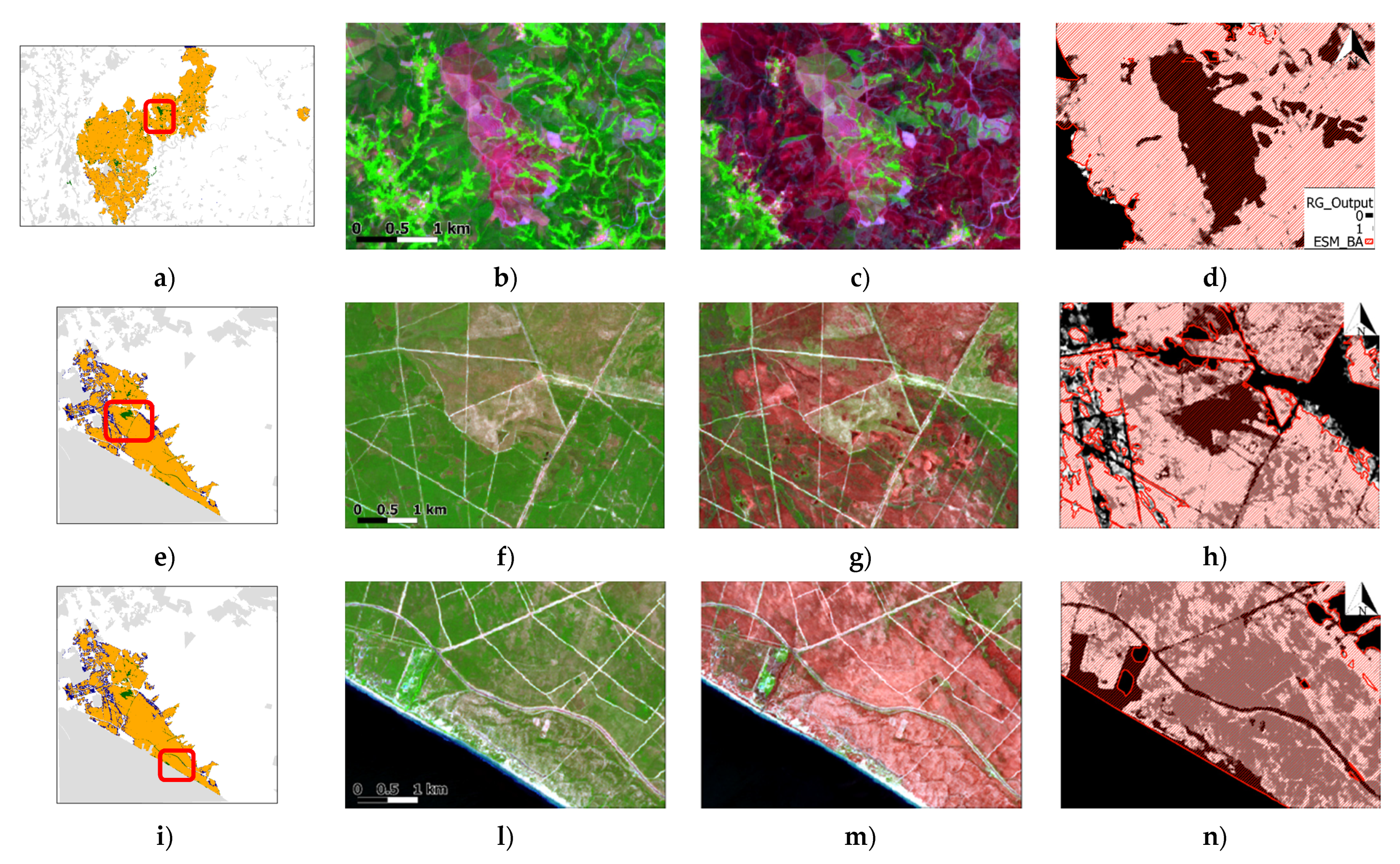
4.4. Exportability Results

The algorithm developed over the Vesuvius site was applied to the sites selected for testing and located in Spain (2), Portugal (1) and Greece (2) with the following criteria:

• Seed layer: OWA_AND;
• Seed selection: OWA_AND > 0.9;
• Growing layers: OWA_Average, OWA_AlmostOR and OWA_OR;
• RG algorithm: OWA_grow > 0;
• Burned area mapping: RG_score > 0.

Figure 9 shows the agreement maps for the five sites and the corresponding accuracy metrics are summarized in Figure 10 and compared to metrics estimated for the training site. Increasing commission errors for OR-like operators (ce > 0.15) are visible in Calar and Huelva sites, Spain. In particular, in the Calar site, the OWA_OR growing layer generates a significantly greater commission error (ce > 0.30) by mistakenly classifying as burned a region of woodland–shrubland located in the northeastern part of the site. Additionally, in the Zakynthos site, Greece, commission error for the OR-like OWA operators is greater than OWA_Average and mainly located in sparsely vegetated land covers. Commission is greater than omission in all sites except Kalamos, Greece, and Leiria, Portugal. In all sites, the difference in the estimates of the Dice coefficient for the three growing layers is negligible while relative bias shows values significantly below zero (overestimation) for Vesuvius, Calar and Huelva sites and OR-like operators confirm the ‘complementary–relaxed’ aggregation of these operators. Estimates of the relative bias clearly show that OWA_Average provides burned area maps that tend to underestimate the area actually burned; again, the opposite occurs for OWA_OR. In terms of relB, the Zakynthos and Leiria sites show the lowest values and no difference among the three growing layers tested. Finally, a negligible difference is observed in accuracy metrics obtained over the Leiria site, Portugal, probably due to the clear burn spectral signal produced by intense and severe fires affecting forest cover; over this site, we obtained the overall greatest Dice coefficient and lowest relative bias.

A regression analysis was carried over a grid layer spacing of 500 m × 500 m to compare the proportion of grid cells labeled as burned in the RG output and the reference maps. This analysis allows a more robust quantitative evaluation of the agreement between classified and reference data [46] by reducing the effect of error compensation. The results are displayed as regression scatter plots and the agreement was quantified by regression coefficients and error metrics: the coefficient of determination (R2) and the root mean squared error (RMSE) computed from the proportion and the total amount (hectares) of area burned within each grid cell (Figure 11). Slopes of the linear regression are generally very close to 1, showing a more than satisfactory agreement between classified and reference maps; in particular, slope values slightly below 1 can be observed for the Leiria, Calar and Kalamos sites, pointing out an underestimation of the area burned in S2 maps; on the contrary, overestimation occurs for the Zakynthos site (slope > 1.07). Indeed, underestimation error is rather expected when burned area mapping is carried out by coarser-resolution data [46] despite the contribution of RG in reducing commission (Figure 12). These trends appear to be least influenced by the OWA_grow layer that is selected in the RG (columns in Figure 11). Only Vesuvius and Huelva show the slope of the regression model changing from negative to positive with OWA_grow; indeed, commission errors brought by the OR-like OWAs lead to a slope > 1. The R2 values confirm the very good agreement with lower values obtained over the Vesuvius training site and with OR-like operators (R2~0.85). By looking at the RMSE, the best results are obtained by applying different OWAs in the different sites: OWA_Average yields the best results in Vesuvius, Huelva and Zakynthos, OWA_OR performs best in Kalamos and Leiria, while OWA_AlmostOR performs best in Calar. Hence, it is not univocally identified which OWA_grow layer performs best across the sites, although OWA_OR should be discarded due to the high overestimation errors. By choosing OWA_Average or OWA_AlmostOR, the average grid cell RMSE is below 2 ha. As highlighted in Figure 9, the greatest commission errors occur over the Calar site, Spain, and with OWA_OR growing layer; this error is represented in the scatter plot by grid cells along the y-axis (BA reference cell proportion = 0).

By observing, in particular, scatter plots for the Leiria and Huelva sites, a large number of grid cells are fully burned according to the reference (BA reference cell proportion along the x-axis = 1) but the burn proportion detected by the RG algorithm is largely variable (BA RG cell proportion along the y-axis) with some cases of full omission. An in-depth analysis of these cells by visual inspection of S2 RGB color composite images (RGB = SWIR − NIR − Red) revealed that disagreement is mainly due to unburned islands and/or linear elements, such as roads, that are included as burned in the EMS polygons. Moreover, discrepancy between RG and reference perimeters is also due to differences in the reference date of the pre-fire image. The EMS pre-fire images can date back to previous years while S2 pre-fire images in this study belong to the same year as the fire event (2017); in fact, to limit the influence of changes of surface conditions due to other phenomena and to maximize the burned/unburned separability, we kept a time gap between pre- and post-fire S2 images in the range of 1–2 months. Some examples area given in the (Appendix A, Figure A4).

5. Discussion

The algorithm described here relies on S2 spectral bands and their temporal difference (pre-fire to post-fire reflectance change) in mapping burned areas in Mediterranean ecosystems. We chose to rely on spectral bands rather than indices for the more robust relationship between reflectance and surface properties; indeed, spectral indices might provide local good discrimination but their performance can vary in space and time [47]. The approach integrates burn evidence from those S2 bands and their temporal differences that showed the greatest sensitivity in discriminating burned and unburned surfaces. Among the S2 spectral bands, the separability metric M identified red–edge (bands 6 and 7) and NIR (band 8) as the most suitable bands while the short-wave infrared domain showed poor separability (M < 1) with the lowest values for SWIR2 (band 12). In this wavelength domain, separability improves slightly above the threshold value (M = 1.1) only when temporal difference (Δ_post-pre) is computed and for the longer wavelength SWIR2 S2 band. Additionally, Δred–edge and NIR reflectance showed high separability (M > 1.5), although lower than post-fire reflectance (M > 1.8), thus, suggesting that, in the case of a lack of temporal series and/or suitable S2 image pairs, single-date images could provide accurate mapping results. This confirms previous findings obtained with Landsat images by Stroppiana et al. (2012) [26].

Seven features (Post_RE2, Post_RE3, Post_NIR, Δ_RE2, Δ_RE3, Δ_NIR, Δ_SWIR2) were therefore selected as input for the algorithm that relies on approximate reasoning to model uncertainty on burned areas through the convergence of evidence of burned conditions. In this framework, pixel-based partial burn evidence is the likelihood of observing burned conditions in a given single spectral feature and the global evidence is given by the complementary–concurrent aggregation of partial evidence degrees. This way, self-adaptation of the algorithm to slightly similar areas and context is achieved, conferring robustness to the approach. Prior to aggregation, input features are interpreted in terms of burn likelihood by membership functions (MFs); similarly to other works proposed in the literature [19], we chose sigmoid-shaped functions to rescale the domain of each input feature into a common domain [0, 1] and these functions were defined from training sets in a semi-automatic way. This improvement makes the implementation of the burned area mapping algorithm less dependent on supervision and/or expert intervention compared to the previous version where membership functions were defined in a fully expert driven way [26]. Tests carried out on the exportability to new sites (4.4) confirmed that MFs are robust and provide reliable results in similar ecological conditions (Mediterranean ecosystems of Southern Europe). If other new regions have similar characteristics in terms of fire regime and land cover, the algorithm could be applied in its present form since it is robust and self-adaptive, stable and valid. The algorithm could be further automatized with MFs defined from training that are automatically extracted, for example, from active fire points in a hybrid approach able to combine multi-source information to add new evidence for burned area classification [10,16].

Integration of partial evidence to derive global scores was achieved with ordered weighted averaging (OWA) operators; OWA layers were then used as input to a region growing (RG) algorithm, which is largely exploited for image segmentation to balance omission and commission errors [25]. An initial seed layer, in which burned pixels are identified to minimize commission errors (i.e., in this case using an AND-like OWA), expands by adding new neighboring pixels belonging to a grow layer, identified to minimize omission errors (i.e., in this case OR-like OWA). The improved performance of the algorithm achieved with RG is presented in Figure 12 for the Vesuvius training site. First, the implementation of the RG combined with OWA significantly reduces relative bias (relB) that quantifies the difference between overestimation and underestimation. Moreover, RG reduces the higher omission error brought by AND-like OWAs (more restrictive conditions on the convergence of evidence) while it reduces commission of the OR-like operators. The balance between these two types of errors, as quantified by the Dice coefficient (dc), shows that RG brings significant improvement with respect to extreme OWA_AND and OWA_OR accuracy (dc~0.6).

Hence, two layers of global evidence were selected as input to the RG algorithm for seed selection and growing. Seeds were identified as pixels where OWA_AND > 0.9 to guarantee the highest reliability relying on the OWA operator able to implement ‘concurrent–strict’ integration conditions. On the other hand, the grow layer is selected among operators implementing “partially complementary–relaxed” (average) and “complementary–relaxed” (OR-like) aggregation. The output of the RG algorithm (RG_score) is a continuous layer in [0, 1] that can be segmented to deliver a binary two-class burned/unburned map to be compared to reference fire perimeters (i.e., validation).

Preliminary analysis over the Vesuvius training site (Appendix A, Figure A2 and Figure A3) showed that all pixels in the OWA_grow layer could be retained as potentially burned (OWA_grow > 0) and all evidence values from the RG algorithm contribute to burned area mapping (RG_score > 0). Under these conditions, estimated accuracy metrics are commission error < 0.22, omission error < 0.15, Dice coefficient > 0.84.

Over the exportability sites, accuracy metrics fall in the range of values: oe [0.02, 0.15], ce [0.01, 0.22], dc [0.84, 0.97] and relB [−0.077, 0.040]. The range of values is given by the three OWAs used as potential layers for growing boundaries. Accuracy metrics are more than satisfactory for a semi-automatic burned area mapping algorithm covering a wide range of fire and land cover conditions in Mediterranean ecosystems. Where fire severity is greatest, such as in the case of the Leiria site, Portugal, we observed that all three growing layers analyzed provided comparable accuracy.

In the literature, Pulvirenti et al. (2020) [48] proposed an automated algorithm based on S2 spectral indices over forest areas and achieved an average commission error of 6.3% and omission error of 12.7%. Similarly, Smiraglia et al. (2020) [49] obtained commission error = 33% and omission error = 24% by also exploiting S2 spectral indices. Furthermore, Seydi et al. (2021) [50] mapped burned areas with a random forest algorithm (proved to be the algorithm providing greatest accuracy) with ce = 8.7% and oe = 9.2%. Hence, the performance of the algorithm proposed here is consistent with published results.

The regression analysis over 500 m × 500 m grid cells confirmed the high spatial accuracy achieved over all sites and, in particular, over Kalamos and Zakynthos, Greece (R2~1, RMSE < 0.1 ha). Overall accuracy metrics (Figure 10) showed that the algorithm tends to overestimate, with commission errors larger than omissions; the greatest overestimation rate being from the OWA_OR (RMSE > 3 ha), as also shown by the agreement maps (Figure 9, third column). In these cases, areas erroneously classified as burned are mainly located in sparsely vegetated land covers. On the contrary, disagreement between reference and S2 classification and resulting in large omission errors occurred in the Leiria and Huelva sites. In these cases, the regression analyses highlighted local omission errors better than the overall accuracy metrics: visual comparison of RGB S2 composite images pointed out that these errors are due to unburned islands and linear patterns (e.g., roads) that are erroneously included in the reference burned polygons. Additionally, differences in pre-fire image date for S2 (our algorithm) and EMS products could lead to biased accuracy metrics; an example is reported in the (Appendix A, Figure A4). Although EMS delineation maps proved to be suitable source of information for validation [18] by delivering reliable fire perimeters in rapid mapping mode, inconsistency might occur locally. Since no detailed information is available on the accuracy of the EMS fire perimeters, we could not further investigate this issue.

From the algorithm point of view, even if a single OWA_grow layer was not identified as the best performing across all sites, we can be confident in stating that OWA_Average and OWA_AlmostOR are the best ones. If the characteristics of a new region are known in advance and comparable to those of one of our test sites, we could select the best OWA case by case.

6. Conclusions

We propose a burned area mapping algorithm that is an improvement over a previous version [26] in several aspects:

• Customization to S2 imagery for implementing a convergence of evidence approach;
• Exploitation of additional spectral bands available from the S2 MSI instrument;
• Automatic interpretation of input features (e.g., post-fire and Δ_post-pre reflectance) through membership functions (MFs) defined from training statistics (partial evidence of burn);
• Tests of OWA operators from AND-like (for seed selection) to OR-like (for growing layer) integration criteria;
• Implementation of OWA global evidence in a region growing (RG) algorithm;
• Accuracy assessment over a wide range of conditions/locations in Southern Europe for the 2017 summer fire season.

Accuracy over training and exportability sites confirmed that the semi-automatic algorithm is robust and self-adaptive over different land cover and fire regime conditions in Mediterranean landscapes. Overall, accuracy metrics (oe < 15%, ce < 22%, dc > 0.84) are consistent with values from the literature for regional applications, although effort should be made in reducing commission errors. A key issue in the validation activity is the availability of reference fire perimeters comparable in space and time with the burned area maps from classification that could induce biased estimation of accuracy metrics. Finally, future activity will be focused on the exploitation of the output burn evidence from OWA operators and RG (RG_score) as an indicator of variable degrees of burn severity.

References

1. Carvalho, A.; Monteiro, A.; Flannigan, M.; Solman, S.; Miranda, A.I.; Borrego, C. Forest fires in a changing climate and their impacts on air quality. Atmos. Environ. 2011, 45, 5545–5553. [Google Scholar] [CrossRef]
2. Knorr, W.; Jiang, L.; Arneth, A. Climate, CO2 and human population impacts on global wildfire emissions. Biogeosciences 2016, 13, 267–282. [Google Scholar] [CrossRef] [Green Version]
3. Jolly, W.M.; Cochrane, M.A.; Freeborn, P.H.; Holden, Z.A.; Brown, T.J.; Williamson, G.J.; Bowman, D.M.J.S. Climate-induced variations in global wildfire danger from 1979 to 2013. Nat. Commun. 2015, 6, 7537. [Google Scholar] [CrossRef] [PubMed]
4. Abatzoglou, J.T.; Williams, A.P.; Barbero, R. Global emergence of anthropogenic climate change in fire weather indices. Geophys. Res. Lett. 2019, 46, 326–336. [Google Scholar] [CrossRef] [Green Version]
5. Dupuy, J.L.; Fargeon, H.; Martin-St Paul, N.; Pimont, F.; Ruffault, J.; Guijarro, M.; Hernando, C.; Madrigal, J.; Fernandes, P. Climate change impact on future wildfire danger and activity in southern Europe: A review. Ann. Forest Sci. 2020, 77, 35. [Google Scholar] [CrossRef]
6. Van der Werf, G.R.; Randerson, J.T.; Giglio, L.; Collatz, G.; Mu, M.; Kasibhatla, P.S.; Morton, D.C.; DeFries, R.S.; Jin, Y.; van Leeuwen, T.T. Global fire emissions and the contribution of deforestation, savanna, forest, agricultural, and peat fires (1997–2009). Atmos. Chem. Phys. 2010, 10, 11707–11735. [Google Scholar] [CrossRef] [Green Version]
7. Yue, C.; Ciais, P.; Cadule, P.; Thonicke, K.; van Leeuwen, T.T. Modelling the role of fires in the terrestrial carbon balance by incorporating SPITFIRE into the global vegetation model ORCHIDEE—part 2: Carbon emissions and the role of fires in the global carbon balance. Geosci. Model Dev. 2015, 8, 1285–1297. [Google Scholar] [CrossRef] [Green Version]
8. Li, F.; Levis, S.; Ward, D.S. Quantifying the role of fire in the Earth system—Part 1: Improved global fire modeling in the Community Earth System Model (CESM1). Biogeosciences 2013, 10, 2293–2314. [Google Scholar] [CrossRef] [Green Version]
9. Li, F.; Bond-Lamberty, B.; Levis, S. Quantifying the role of fire in the Earth system—Part 2: Impact on the net carbon balance of global terrestrial ecosystems for the 20th century. Biogeosciences 2014, 11, 1345–1360. [Google Scholar] [CrossRef] [Green Version]
10. Alonso-Canas, I.; Chuvieco, E. Global burned area mapping from ENVISAT-MERIS and MODIS active fire data. Remote Sens. Environ. 2015, 163, 140–152. [Google Scholar] [CrossRef]
11. Libonati, R.; DaCamara, C.; Setzer, A.; Morelli, F.; Melchiori, A. An algorithm for burned area detection in the Brazilian cerrado using 4 µm MODIS imagery. Remote Sens. 2015, 7, 15782–15803. [Google Scholar] [CrossRef] [Green Version]
12. Chuvieco, E.; Mouillot, F.; van der Werf, G.R.; San Miguel, J.; Tanase, M.; Koutsias, N.; García, M.; Yebra, M.; Padilla, M.; Gitas, I.; et al. Historical background and current developments for mapping burned area from satellite earth observation. Remote Sens. Environ. 2019, 225, 45–64. [Google Scholar] [CrossRef]
13. Giglio, L.; Schroeder, W.; Justice, C.O. The collection 6 MODIS active fire detection algorithm and fire products. Remote Sens. Environ. 2016, 178, 31–41. [Google Scholar] [CrossRef] [PubMed] [Green Version]
14. Shimabukuro, Y.E.; Dutra, A.C.; Arai, E.; Duarte, V.; Cassol, H.L.G.; Pereira, G.; Cardozo, F.S. Mapping burned areas of mato grosso state Brazilian amazon using multisensor datasets. Remote Sens. 2020, 12, 3827. [Google Scholar] [CrossRef]
15. Chuvieco, E.; Yue, C.; Heil, A.; Mouillot, F.; Alonso-Canas, I.; Padilla, M.; Pereira, J.M.; Oom, D.; Tansey, K. A new global burned area product for climate assessment of fire impacts. Glob. Ecol. Biogeogr. 2016, 25, 619–629. [Google Scholar] [CrossRef] [Green Version]
16. Pereira, A.A.; Pereira, J.M.C.; Libonati, R.; Oom, D.; Setzer, A.W.; Morelli, F.; Machado-Silva, F.; de Carvalho, L.M.T. Burned area mapping in the Brazilian savanna using a one-class support vector machine trained by active fires. Remote Sens. 2017, 9, 1161. [Google Scholar] [CrossRef] [Green Version]
17. Randerson, J.T.; Chen, Y.; van der Werf, G.R.; Rogers, B.M.; Morton, D.C. Global burned area and biomass burning emissions from small fires. Biogeoscience 2012, 117. [Google Scholar] [CrossRef]
18. Filipponi, F. Exploitation of sentinel-2 time series to map burned areas at the national level: A case study on the 2017 Italy wildfires. Remote Sens. 2019, 11, 622. [Google Scholar] [CrossRef] [Green Version]
19. Roteta, E.; Bastarrika, A.; Padilla, M.; Storm, T.; Chuvieco, E. Development of a sentinel-2 burned area algorithm: Generation of a small fire database for sub-Saharan Africa. Remote Sens. Environ. 2019, 222, 1–17. [Google Scholar] [CrossRef]
20. Stavrakoudis, D.; Katagis, T.; Minakou, C.; Gitas, I.Z. Automated burned scar mapping using sentinel-2 imagery. J. Geogr. Inf. Syst. 2020, 12, 221–240. [Google Scholar] [CrossRef]
21. Roy, D.; Huang, H.; Boschetti, L.; Giglio, L.; Yan, L.; Zhang, H.; Li, Z. Landsat-8 and Sentinel-2 burned area mapping—a combined sensor multi-temporal change detection approach. Remote Sens. Environ. 2019, 231, 111254. [Google Scholar] [CrossRef]
22. Boschetti, L.; Roy, D.; Justice, C.O.; Michael, L.; Humber, M.L. MODIS–Landsat fusion for large area 30 m burned area mapping. Remote Sens. Environ. 2015, 161, 27–42. [Google Scholar]
23. Li, J.; Roy, D.P. A Global analysis of sentinel-2a, sentinel-2b andlandsat-8 data revisit intervals and implications for terrestrial monitoring. Remote Sens. 2017, 9, 902. [Google Scholar] [CrossRef] [Green Version]
24. Liu, S.; Zheng, Y.; Dalponte, M.; Tong, X. A novel fire index-based burned area change detection approach using Landsat-8 OLI data. Eur. J. Remote Sens. 2020, 53, 104–112. [Google Scholar] [CrossRef] [Green Version]
25. Bastarrika, A.; Chuvieco, E.; Martín, M.P. Mapping burned areas from Landsat TM/ETM+ data with a two-phase algorithm: Balancing omission and commission errors. Remote Sens. Environ. 2011, 115, 1003–1012. [Google Scholar] [CrossRef]
26. Stroppiana, D.; Bordogna, G.; Carrara, P.; Boschetti, M.; Boschetti, L.; Brivio, P.A. A method for extracting burned areas from Landsat TM/ETM+ images by soft aggregation of multiple Spectral Indices and a region growing algorithm. ISPRS J. Photogramm. Remote Sens. 2012, 69, 88–102. [Google Scholar] [CrossRef]
27. Goffi, A.; Stroppiana, D.; Brivio, P.A.; Bordogna, G.; Boschetti, M. Towards an automated approach to map flooded areas from Sentinel-2 MSI data and soft integration of water spectral features. Int. J. Appl. Earth Obs. 2020, 84, 101951. [Google Scholar] [CrossRef]
28. Yager, R.R. On ordered weighted averaging aggregation operators in multi-criteria decision making. IEEE Trans. Syst. Man Cybern. 1988, 18, 183–190. [Google Scholar] [CrossRef]
29. Sánchez-Benítez, A.; García-Herrera, R.; Barriopedro, D.; Sousa, P.M.; Trigo, R.M. June 2017: The earliest european summer mega-heatwave of reanalysis period. Geophys. Res. Lett. 2018, 45, 1955–1962. [Google Scholar] [CrossRef]
30. Turco, M.; Jerez, S.; Augusto, S.; Tarin-Carrasco, P.; Ratola, N.; Jimenez-Guerrero, P.; Trigo, R.M. Climate drivers of the 2017 devastating fires in Portugal. Sci. Rep. 2019, 9, 13886. [Google Scholar] [CrossRef]
31. Ranghetti, L.; Busetto, L. Sen2r: An R Toolbox to Find, Download and Preprocess Sentinel-2 Data. R Package Version 1.0.0. 2019. Available online: http://sen2r.ranghetti.info (accessed on 1 May 2021).
32. Main-Knorn, M.; Pflug, B.; Louis, J.; Debaecker, V.; Müller-Wilm, U.; Gascon, F. Sen2Cor for sentinel-2. In Proceedings of the SPIE 10427, Image and Signal Processing for Remote Sensing XXIII, Warsaw, Poland, 10–14 September 2017; p. 1042704. [Google Scholar]
33. Louis, J.; Charantonis, A.; Berthelot, B. Cloud detection for sentinel-2. In Proceedings of the ESA Living Planet Symposium, Bergen, Norway, 28 June–2 July 2010. [Google Scholar]
34. Planet Team. Planet Application Program Interface: In Space for Life on Earth. San Francisco, CA. 2017. Available online: https://api.planet.com (accessed on 1 May 2021).
35. Lemajic, S.; Vajsová, B.; Aastrand, P. New Sensors Benchmark Report on PlanetScope: Geometric Benchmarking Test for Common Agricultural Policy (CAP) Purposes; Publications Office of the European Union: Luxembourg, 2018; ISBN 978-92-79-92833-8. JRC111221. [Google Scholar] [CrossRef]
36. Belgiu, M.; Drăguţ, L. Random forest in remote sensing: A review of applications and future directions. ISPRS J. Photogramm. Remote Sens. 2016, 114, 24–31. [Google Scholar] [CrossRef]
37. Ramo, R.; Chuvieco, E. Developing a random forest algorithm for MODIS global burned area classification. Remote Sens. 2017, 9, 1193. [Google Scholar] [CrossRef] [Green Version]
38. Breiman, L. Random forest. Mach. Learn. 2001, 45, 5–32. [Google Scholar] [CrossRef] [Green Version]
39. Boschetti, M.; Nutini, F.; Manfron, G.; Brivio, P.A.; Nelson, A. Comparative analysis of normalised difference spectral indices derived from MODIS for detecting surface water in flooded rice cropping systems. PLoS ONE 2014, 9, e88741. [Google Scholar] [CrossRef] [PubMed]
40. Carrara, P.; Bordogna, G.; Boschetti, M.; Brivio, P.A.; Nelson, A.; Stroppiana, D. A flexible multi-source spatial-data fusion system for environmental status assessment at continental scale. Int. J. Geogr. Inf. Sci. 2008, 22, 781–799. [Google Scholar] [CrossRef]
41. Goffi, A.; Bordogna, G.; Stroppiana, D.; Boschetti, M.; Brivio, P.A. Knowledge and data-driven mapping of environmental status indicators from remote sensing and VGI. Remote Sens. 2020, 12, 495. [Google Scholar] [CrossRef] [Green Version]
42. Congalton, R.G.; Green, K. Assessing the Accuracy of Remotely Sensed Data, 2nd ed.; CRC Press: Boca Raton, FL, USA, 2008; p. 346. [Google Scholar]
43. Roy, D.P.; Jin, Y.; Lewis, P.E.; Justice, C.O. Prototyping a global algorithm for systematic fire-affected area mapping using MODIS time series data. Remote Sens. Environ. 2005, 97, 137–162. [Google Scholar] [CrossRef]
44. Clevers, J.G.; Gitelson, A.A. Remote estimation of crop and grass chlorophyll and nitrogen content using red-edge bands on Sentinel-2 and -3. Int. J. Appl. Earth Obs. Geoinf. 2013, 23, 344–351. [Google Scholar] [CrossRef]
45. Saulino, L.; Rita, A.; Migliozzi, A.; Maffei, C.; Allevato, E.; Garonna, A.P.; Saracino, A. Detecting burn severity across mediterranean forest types by coupling medium-spatial resolution satellite imagery and field data. Remote Sens. 2020, 12, 741. [Google Scholar] [CrossRef] [Green Version]
46. Boschetti, L.; Roy, D.P.; Giglio, L.; Huang, H.; Zubkova, M.; Humber, M.L. Global validation of the collection 6 MODIS burned area product. Remote Sens. Environ. 2019, 235, 111490. [Google Scholar] [CrossRef]
47. Huang, H.; Roy, D.P.; Boschetti, L.; Zhang, H.K.; Yan, L.; Kumar, S.S.; Gomez-Dans, J.; Li, J. Separability analysis of sentinel-2a multi-spectral instrument (MSI) data for burned area discrimination. Remote Sens. 2016, 8, 873. [Google Scholar] [CrossRef] [Green Version]
48. Pulvirenti, L.; Squicciarino, G.; Fiori, E.; Fiorucci, P.; Ferraris, L.; Negro, D.; Gollini, A.; Severino, M.; Puca, S. An automatic processing chain for near real-time mapping of burned forest areas using sentinel-2 data. Remote Sens. 2020, 12, 674. [Google Scholar] [CrossRef] [Green Version]
49. Smiraglia, D.; Filipponi, F.; Mandrone, S.; Tornato, A.; Taramelli, A. Agreement index for burned area mapping: Integration of multiple spectral indices using sentinel-2 satellite images. Remote Sens. 2020, 12, 1862. [Google Scholar] [CrossRef]
50. Seydi, S.T.; Akhoondzadeh, M.; Amani, M.; Mahdavi, S. Wildfire damage assessment over Australia using sentinel-2 imagery and MODIS land cover product within the google earth engine cloud platform. Remote Sens. 2021, 13, 220. [Google Scholar] [CrossRef]
Figure 1. The CLC2012 land cover classes over the six sites located in Southern Europe (a): Vesuvius, Italy (b), Leiria, Portugal (c), Calar, Spain (d), Huelva, Spain (e), Kalamos, Greece (f), Zakynthos, Greece (g).
Remotesensing 13 02214 g001
Figure 2. Pre- and post-fire S2 images (first and second column) and EMS fire grading maps (last column) for each site: Vesuvius, Italy, (ac); Leiria, Portugal, (df); Calar, Spain (gi); Huelva, Spain (jl); Kalamos, Greece (mo); Zakynthos, Greece (pr). S2 images are displayed as RGB false color composites (SWIR2, NIR, red). Notice that for Kalamos and Zakynthos sites, Greece, no fire damage grading maps are available from EMS.
Remotesensing 13 02214 g002aRemotesensing 13 02214 g002b
Figure 3. Pre- (a) and post-fire (b) PlanetScope images: 22 April and 22 July 2017, over the Vesuvius sites. Images are displayed as RGB false color composites (NIR, red, green) and the reference burned area map (c) obtained with RF algorithm. Black polygon shows the border of Vesuvius National Park.
Remotesensing 13 02214 g003
Figure 4. The s-shaped (a) and z-shaped (b) sigmoid functions chosen as MFs to quantify the partial evidence of burn.
Remotesensing 13 02214 g004
Figure 5. Flowchart of the processing steps from input S2 MSI images to generate BA maps.
Remotesensing 13 02214 g005
Figure 6. Partial evidence of burn as given by the input features interpreted by sigmoid MFs: PostRE2 (a), PostRE3 (b) PostNIR (c), ΔRE2 (d), ΔRE3 (e), ΔNIR (f) and ΔSWIR2 (g). Color scale shows increasing degree and likelihood of burn (blue to yellow).
Remotesensing 13 02214 g006
Figure 7. Global evidence of burn shown by OWA score [0, 1] (left column) over the Vesuvius study site: OWAAND (a), OWAalmostAND (b), OWAAverage (c), OWAAlmostOR (d) and OWAOR (e); borders of Vesuvius National Park are highlighted in black and masked areas in gray.
Remotesensing 13 02214 g007
Figure 8. RGscore and agreement maps for the Vesuvius training site for growing layers OWAAverage (a,d), OWAAlmostOR (b,e) and OWAOR (c,f).
Remotesensing 13 02214 g008
Figure 9. Agreement maps obtained for OWAAverage (left column), OWAAlmostOR (middle column) and OWAOR (right column) over exportability sites: Leiria, Portugal (ac), Calar, Spain (df), Huelva, Spain (gi), Kalamos, Greece (ln) and Zakynthos, Greece (oq). The four classes represent: correctly classified burned pixels (orange), correctly classified unburned pixels (white), pixels mistakenly classified as burned—commission (blue) and pixel mistakenly classified as unburned—omission (green).
Remotesensing 13 02214 g009aRemotesensing 13 02214 g009b
Figure 10. Accuracy metrics (omission error = oe, commission error = ce, Dice coefficient = dc and relative bias = relB) over the exportability and training sites.
Remotesensing 13 02214 g010
Figure 11. Scatter plot of the proportion of 500 m × 500 m grid cell mapped as burned in the RG output and the reference dataset for each site and OWAgrow layer. Scatter plots are displayed as counts of cells for 0.05 step along the x- and y-axis to better represent overlapping points and with a logarithmic color scale. The black dotted line is the 1:1 line while the gray continuous line is the linear regression model. The coefficient of determination (R2), slope of the regression linear model (Slope), root mean squared error (RMSE) and total number of cells (N cells) are also shown.
Remotesensing 13 02214 g011
Figure 12. Accuracy metrics (omission error = oe, commission error = ce, Dice coefficient = dc and relative bias = relB) over the training site for burned area maps obtained with the RG algorithm (with three cases of growing layer, OWAAverage, OWAAlmost_OR and OWAOR) and from segmentation of the OWA global evidence (from all tested OWAs).
Remotesensing 13 02214 g012