Article

Enhancement of Detecting Permanent Water and Temporary Water in Flood Disasters by Fusing Sentinel-1 and Sentinel-2 Imagery Using Deep Learning Algorithms: Demonstration of Sen1Floods11 Benchmark Datasets

1
Center for Applied Statistics, School of Statistics, Renmin University of China, Beijing 100872, China
2
China Huaneng Group Co., Ltd., Beijing 100031, China
3
Graduate School of Information Science and Technology, The University of Tokyo, Tokyo 113-8656, Japan
4
School of Informatics, The University of Edinburgh, Edinburgh EH8 9AB, UK
5
Graduate School of Information Sciences, Tohoku University, Sendai 980-8579, Japan
6
International Research Institute of Disaster Science, Tohoku University, Sendai 980-8572, Japan
*
Author to whom correspondence should be addressed.
These authors contributed equally to this work.
Remote Sens. 2021, 13(11), 2220; https://0-doi-org.brum.beds.ac.uk/10.3390/rs13112220
Submission received: 10 May 2021 / Revised: 1 June 2021 / Accepted: 2 June 2021 / Published: 5 June 2021

Abstract

:
Identifying permanent water and temporary water in flood disasters efficiently has mainly relied on change detection method from multi-temporal remote sensing imageries, but estimating the water type in flood disaster events from only post-flood remote sensing imageries still remains challenging. Research progress in recent years has demonstrated the excellent potential of multi-source data fusion and deep learning algorithms in improving flood detection, while this field has only been studied initially due to the lack of large-scale labelled remote sensing images of flood events. Here, we present new deep learning algorithms and a multi-source data fusion driven flood inundation mapping approach by leveraging a large-scale publicly available Sen1Flood11 dataset consisting of roughly 4831 labelled Sentinel-1 SAR and Sentinel-2 optical imagery gathered from flood events worldwide in recent years. Specifically, we proposed an automatic segmentation method for surface water, permanent water, and temporary water identification, and all tasks share the same convolutional neural network architecture. We utilize focal loss to deal with the class (water/non-water) imbalance problem. Thorough ablation experiments and analysis confirmed the effectiveness of various proposed designs. In comparison experiments, the method proposed in this paper is superior to other classical models. Our model achieves a mean Intersection over Union (mIoU) of 52.99 % , Intersection over Union (IoU) of 52.30 % , and Overall Accuracy (OA) of 92.81 % on the Sen1Flood11 test set. On the Sen1Flood11 Bolivia test set, our model also achieves very high mIoU ( 47.88 % ), IoU ( 76.74 % ), and OA ( 95.59 % ) and shows good generalization ability.

Graphical Abstract

1. Introduction

Natural hazards such as floods, landslides, and typhoons pose severe threats to people’s lives and property. Among them, floods are the most frequent, widespread, and deadly natural disasters. They affect more people globally each year than any other disaster [1,2,3]. Floods not only cause injuries, deaths, losses of livelihoods, infrastructure damage, and asset losses, but they can also have direct or indirect effects on health [4]. In the past decade, there have been 2850 disasters that triggered natural hazards globally, of which 1298 were floods, accounting for approximately 46 % [1]. In 2019, there were 127 floods worldwide, affecting 69 countries, causing 1586 deaths and more than 10 million displacements [2]. In the future, floods may become a frequent disaster that poses a huge threat to human society due to sea-level rise, climate change, and urbanization [5,6].
The effective way to reduce flood losses is to enhance our ability of flood risk mitigation and response. In recent years, timely and accurate flood detection products derived from satellite remote sensing imagery are becoming effective methods of responding flood disaster, and city and infrastructure planners, risk managers, disaster emergency response agency, and property insurance company are benefiting from it in worldwide [7,8,9,10,11], while identifying permanent water and temporary water in flood disasters efficiently is a remaining challenge.
In recent years, researchers have done a lot of work in flood detection based on satellite remote sensing images. The most commonly used method to distinguish between water and non-water areas is a threshold split-based method [12,13,14,15]. However, the optimal threshold is affected by the geographical area, time, and atmospheric conditions of image collection. Therefore, the generalization ability of the above methods is greatly limited. In recent years, the European Space Agency (ESA) developed a series of Sentinel missions to provide free available datasets including Synthetic Aperture Radar (SAR) data from Sentinel-1 sensor and optical data from Sentinel-2 sensor, taking into account the respective advantages of optical imagery and SAR imagery in flood information extraction [5,14,16,17,18], and the investigation of combining SAR images with optical images for more accurate flood mapping is of great interest for researchers [16,19,20,21,22]. Although the data fusion method improves the accuracy of flood extraction, it is still very challenging to distinguish permanent water from temporary water problems in flood disasters. The identification of temporary waters in flood disasters and permanent waters mainly rely on multi-temporal change detection methods [23,24,25,26,27,28]. This type of approach requires at least one pair of multi-temporal remote sensing scenes which were acquired before and after a flood event. Although the method based on multi-temporal change detection can better detect the temporary water in flood disaster events, the multi-temporal method was greatly limited due to the mandatory demand for satellite imagery before disasters.
Deep learning methods represented by convolutional neural networks have been proven to be effective in the field of flood damage assessment, and related research has grown rapidly since 2017 [29]. However, most algorithms are focusing on affected buildings in flood events [22,30], with very few examples of flood water detection. The latest research focuses on the application of deep learning algorithms for enhancing flood water detection [31,32]. Early research focused on the extraction of surface water [33,34,35]. Furkan et al. proposed a deep-learning-based approach for surface water mapping from Landsat imagery. The results demonstrated that the deep learning method outperform the traditional threshold and Multi-Layer Perceptron model. Considering the difference in the characteristics of surface water and floods in satellite imagery, which will increase the difficulty of flood extraction. Maryam et al. developed a semantic segmentation method for extracting the flood boundary from UAV imagery. The semantic segmentation-based flood extraction method was further applied to identify the flood inundation caused by mounting destruction [36]. Experimental results validate the efficiency and effectiveness of the proposed method. Muñoz et al. [37] combined the multispectral Landsat imagery and dual-polarized synthetic aperture radar imagery to evaluate the performance of integrating convolutional neural network and data fusion framework for generating compound flood mapping. The usefulness of this method was verified by comparing with other methods. These studies show that deep learning algorithms play an important role in enhancing flood classification. However, research in this field is still in its infancy, due to the lack of high-quality large-scale flood annotation satellite datasets.
Recent development in earth observation has contributed a series of open-sourced large scale disaster related satellite imagery datasets, which has greatly spurred the advance of leveraging deep learning algorithm for disaster mapping from satellite imagery. For building damage classification, the xBD dataset has provided large scale satellite imagery data that collected from the multi-type disasters with four category damage level labels to worldwide researchers, and the research spawned by this public data has also verified the great potential of deep learning in building damage recognition [38,39]. For flooded building damage assessment in Hurricane disaster events, FloodNet provides a high-resolution UAV image dataset and has done the same task [40]. The recent release of the large-scale open-source Sen1Floods11 dataset [5] is boosting the research of utilizing deep learning algorithms for water type detection in flood disasters [41]. For water type detection in flood disaster events, Sen1Flood should take on a similar role. Unfortunately, so far, only one preliminary work has been conducted.
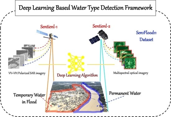
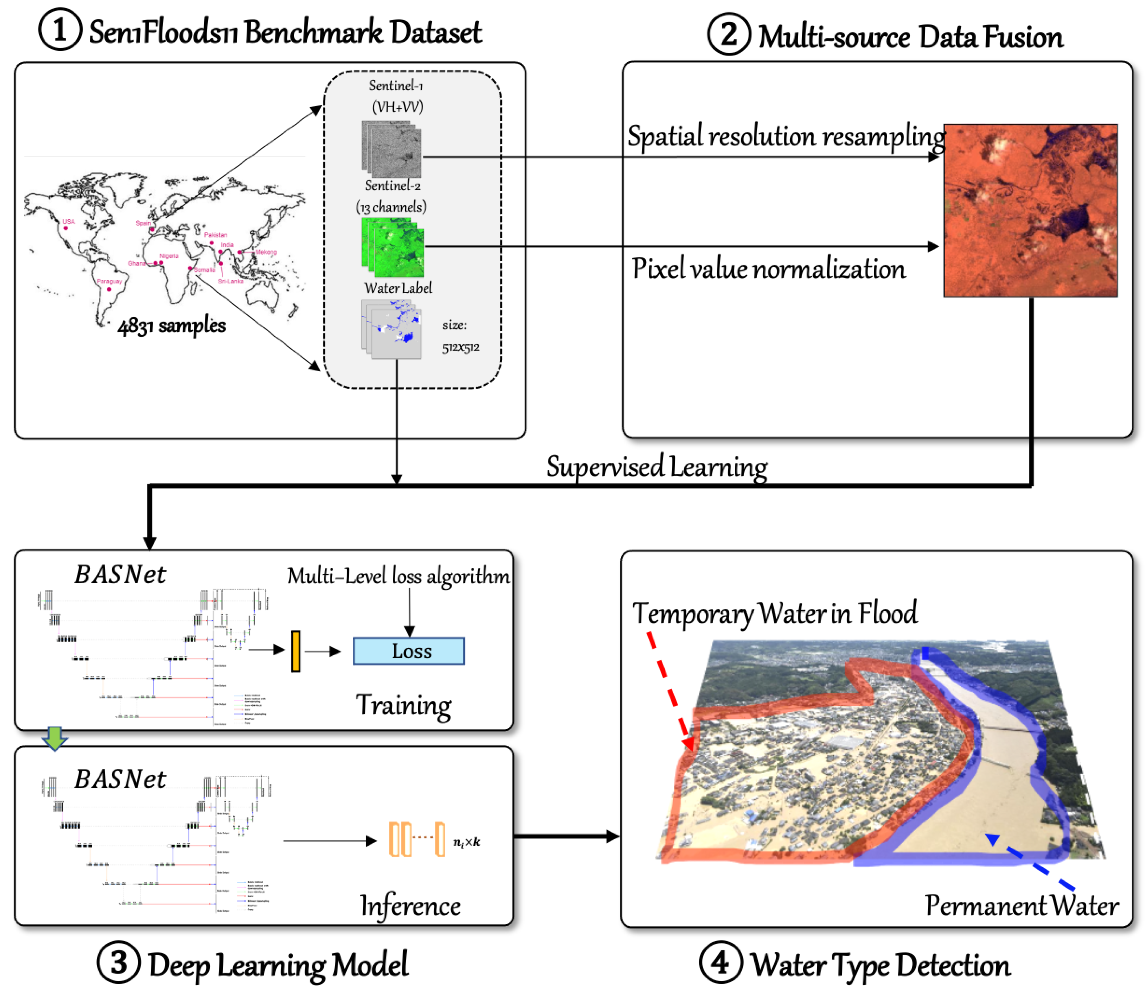
With the purpose of developing an efficient benchmark algorithm for distinguishing between permanent water and temporary water in flood disasters based on the Sen1Flood dataset to boost the research in this area, the contributions and originality of this research are as follows.
  • Effectiveness: To the best of our knowledge, in terms of the sen1flood11 dataset, the accuracy of our proposed algorithm is the highest so far.
  • Convenience: All of the sentinel-1 and sentinel-2 imagery utilized in the model come from post-flood imagery, and this greatly reduces the reliance on satellite imagery data before the flood.
  • Refinement: We introduced salient object detection algorithm to modify the convolutional neural network classifier, in addition, the multi-scale loss algorithm and data augmentation were adopted to improve the accuracy of the model.
  • Robustness: the robustness of our proposed algorithm was verified in a new Bolivia flood dataset.

2. Sen1Floods11 Dataset

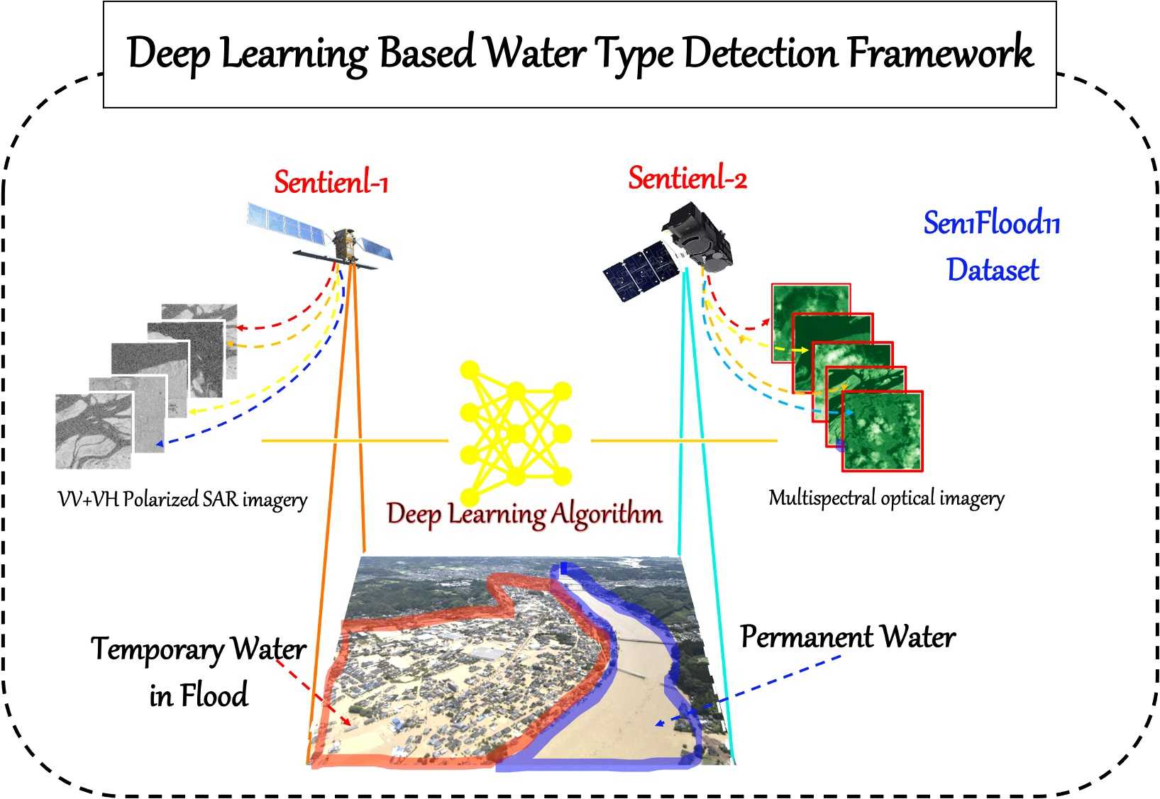
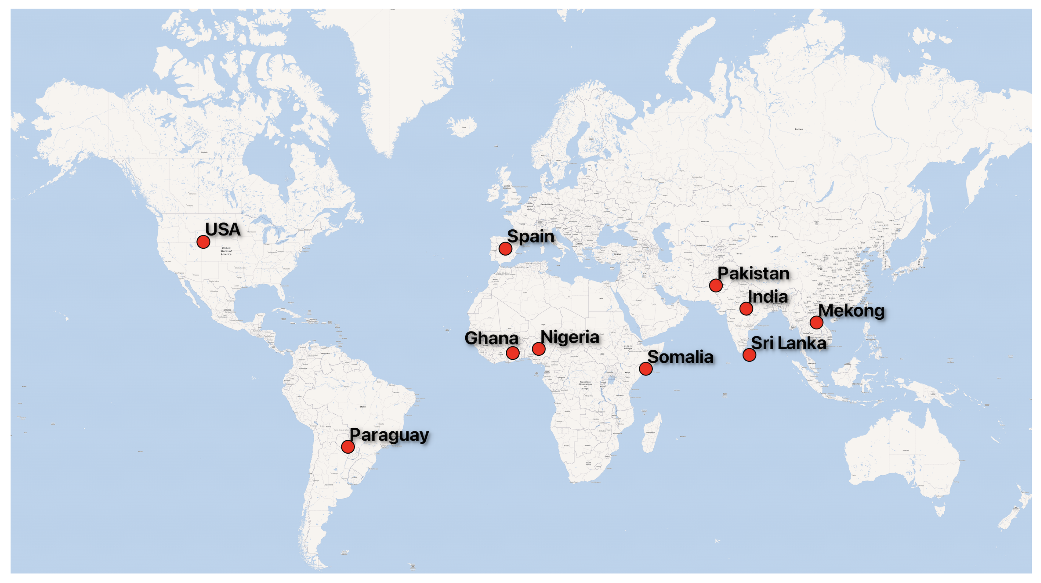
We utilize the Flood Event Data in the Sen1Floods11 dataset [5] to train, validate, and test deep learning flood algorithms. This dataset provides raw Sentinel-1 SAR images (IW mode, GRD product), Sentinel-2 MSI Level-1C images, classified permanent water, and flood water. There are 4831 non-overlapping 512 × 512 tiles from 11 flood events. This dataset helps map flood at the global scale, covering 120,406 square kilometers, spanning 14 biomes, 357 ecological regions, and six continents. Locations for flood events are shown in Figure 1.
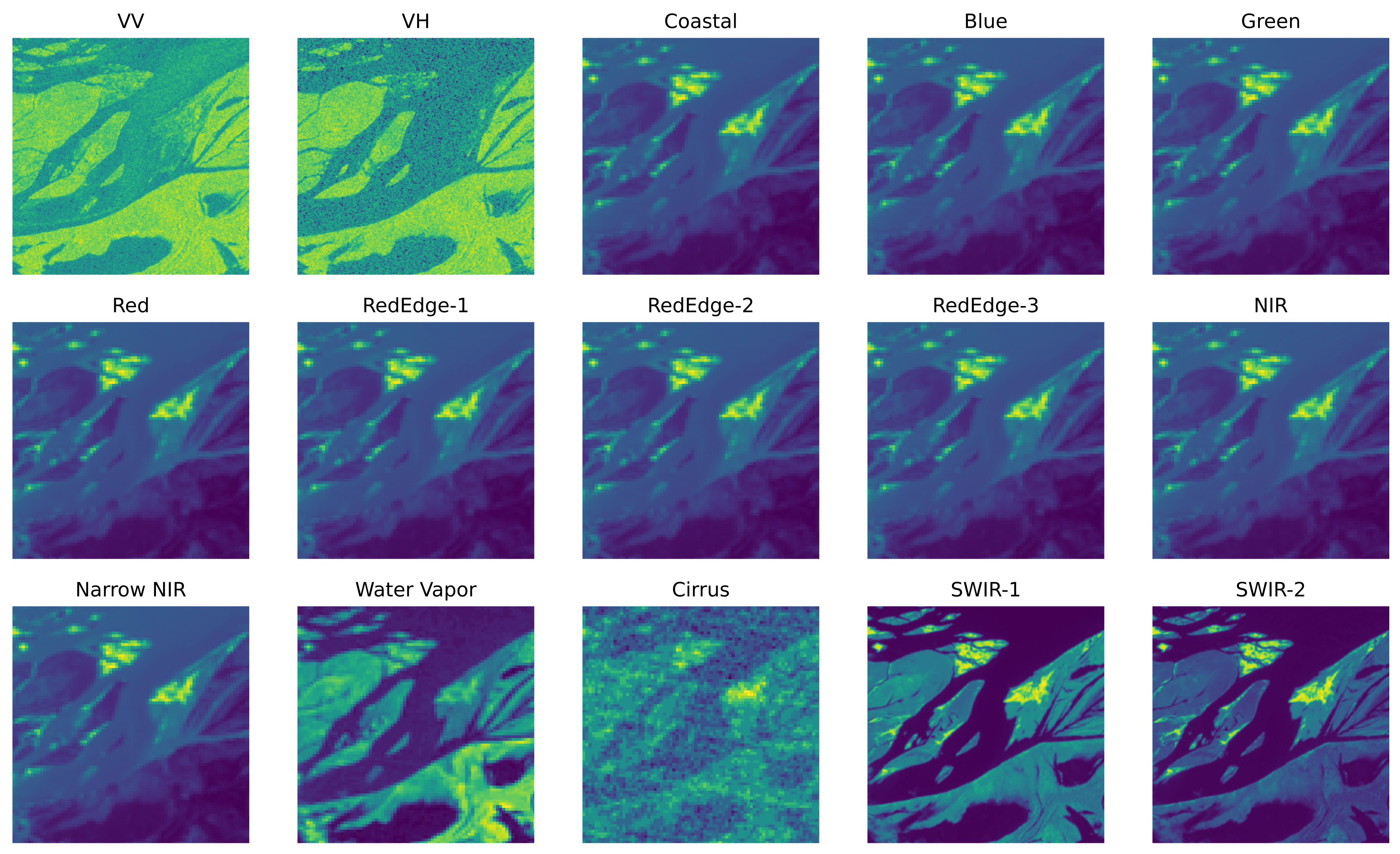
For each selected flood event, the time interval between the acquisition of Sentinel-1 imagery and Sentinel-2 imagery shall not exceed two days. The Sentinel-1 imagery contains two bands, VV and VH, which are backscatter values; the Sentinel-2 imagery includes 13 bands, and all bands are TOA reflectance values. The imagery is projected to the WGS-84 coordinate system.The ground resolution of the imagery is different on different bands. In order to fuse images, the ground resolution is sampled to 10 m on all bands. Each band is visualized in Figure 2.
Due to the high cost of hand labels, 4370 tiles are not hand-labeled and exported with annotations automatically generated by the Sentinel-1 and Sentinel-2 flood classification algorithms, which can serve as weakly supervised training data. The remaining 446 tiles are manually annotated by trained remote sensing analysts for high-quality model training, validation and testing. The weakly supervised data contain two types of surface water labels. One is produced by the histogram thresholding method based on the Sentinel-1 image; the other is generated by the Normalized Difference Vegetation Index (NDVI), MNDWI and thresholding method based on the Sentinel-2 image. All cloud and cloud shadow pixels were masked and excluded from training and accuracy assessments. Hand labels include all water labels and permanent water labels. For all water labels, analysts exploited Google Earth Engine to correct the automated labels using Sentinel-1 VH band, two false color composites from Sentinel-2 and the reference water classification from Sentinel-2 by removing uncertain areas and adding to the water classification. For the permanent water label, with the help of the JRC (European Commission Joint Research Center) surface water data set, Bonafilia et al. [
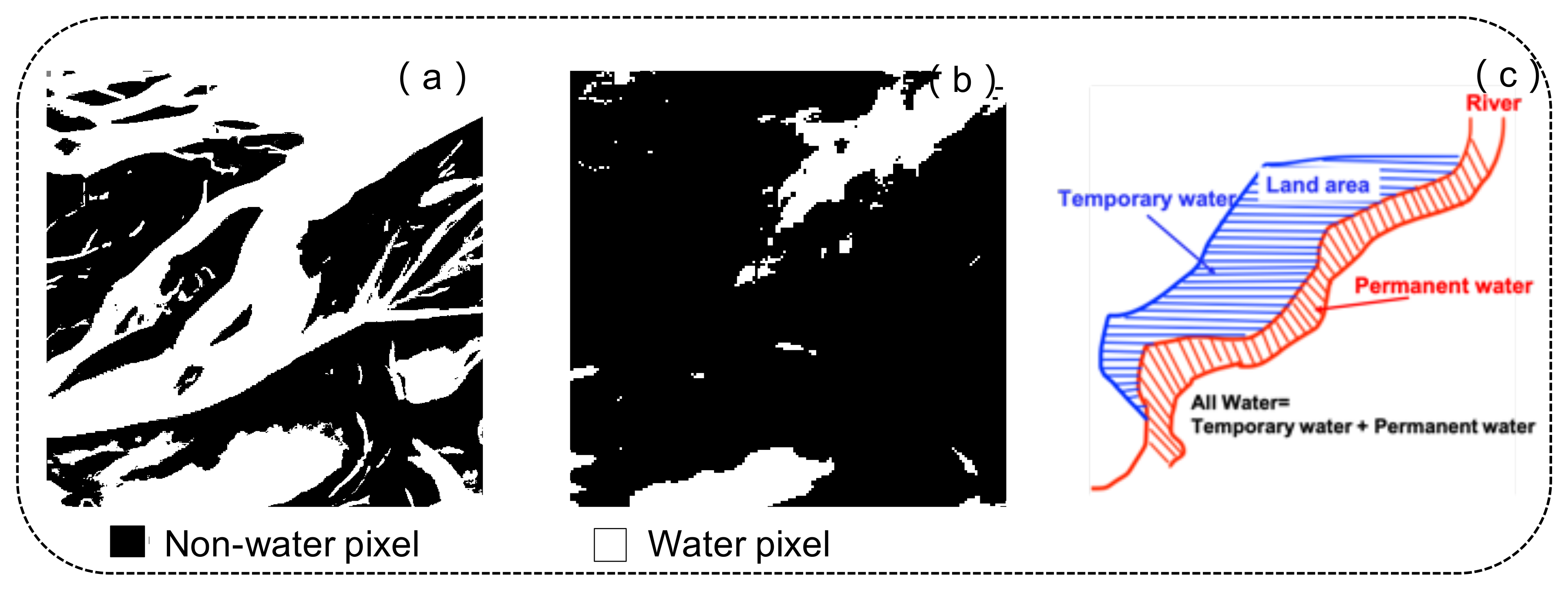
5] labeled the pixels that were detected as water at both the beginning (1984) and end (2018) of the dataset as permanent water pixels. The pixels never observed as water during this period are treated as non-water pixels. The remaining pixels are masked. Examples of water label are visualized in Figure 3.
Like most existing studies [42], the Sen1Floods11 dataset shows the highly imbalanced distribution between flooded and unflooded area. As shown in Table 1, for all water, water pixels account for only 9.16 % , and non-water pixels account for 77.22 % , which is about eight times the number of surface water pixels. The percentages of water pixels and non-water pixels in permanent waters are 3.06 % and 96.94 % , respectively, and the number of non-water pixels is about 32 times that of non-water pixels.
The dataset is split into three parts: training set, validation set, and test set. All 4370 images automatically labeled are used as the weakly supervised training set. The hand-labeled data are first randomly split into training, validation, and testing data in the proportion 6:2:2. In order to test the model’s ability to predict unknown flood events, all hand-labeled data related to the Bolivia flood event is held out for a distinct test set. Rest hand-labeled data in training, validation, and testing sets are composed of final training, validation, and testing set, respectively. Correspondingly, all data from Bolivia in the weakly-supervised training set are also excluded and do not participate in model training. The overall composition of the dataset is shown in Table 2.

3. Method

Figure 4 depicts a flowchart of our work. In this work, the benchmark Sen1Floods11 dataset that contains 4831 samples with 512 × 512-pixel size from both Sentinel-1 and Sentinel-2 imagery were utilized to develop the algorithm. The spatial resolution resampling and pixel value normalization were adopted to fuse sentinel-1 and sentinel-2 imagery. The model input is a stack of fused image bands with permanent water and temporary water annotations. The network used is BASNet proposed by Qin et al. [43] is used. BASNet architecture is shown in Figure 5. The network combines a densely supervised encoder–decoder network similar to U-Net and a new residual refinement module. The encoder–decoder produces a coarse probability prediction map from the image input, and the Residual Refinement Module is responsible for learning the residuals between the coarse probability prediction map and the ground truth. We apply the network to remote sensing data sets, adapt, train, and optimize it to better predict flood areas.

3.1. Encoder–Decoder Network

The encoder–decoder network can fuse abstract high-level information and detailed low-level information and is mainly responsible for water body segmentation. The encoder part contains an input convolution block and six convolution stages consisting of basic res-blocks. The input convolution block comprises a convolution layer with batch normalization [44] and Rectified Linear Unit (ReLU) activation function [45]. The size of the convolution kernel is 3 × 3, and the stride is 1. This convolution block can convert an input image of any number of channels to a feature map of 64 channels. The first four convolution stages directly use the four stages of ResNet34 [46]. Except for the first residual block, each residual block will double the feature map’s channels. The last two convolution stages have the same structure, and both consist of three basic res-blocks with 512 filters and a 2 × 2 max pooling operation with stride 2 for downsampling.
Compared with traditional convolution, atrous convolution can obtain a larger receptive field without increasing parameter amount and capture long-range information. In addition, atrous convolution can avoid the reduction of feature map resolution caused by repeated downsampling and allow a deeper model [47,48]. To capture global information, Qin et al. [43] designed a bridge stage to connect the encoder and the decoder. This stage is comprised of three atrous convolution blocks. Each atrous convolution block consists of a convolution layer with 512 atrous 3 × 3 filters with dilation 2, a batch normalization, and a ReLU activation function.
In the decoder part, each decoder stage corresponds to an encoder stage. As shown in the Formulas (1) and (2), g i is the merge base, f i is the feature map to be fused, h i is the merged feature map, and c o n v 3 × 3 is a convolution layer followed by batch normalization and ReLU activation, RRM represents the Residual Refinement Module and the operator [ · ; · ] represents concatenation along the channel axis. There are three convolution layers with batch normalization and a ReLU activation function in each decoder stage. The feature map from the last stage is first fed to an up-sampling layer to get g i + 1 , and then concatenated with the current feature map f i . In order to alleviate overfitting, the last layer of the bridge stage and each stage of the encoder is fed to a 3 × 3 convolution layer followed by a bilinear up-sampling layer and sigmoid activation function to generate a prediction map and then supervised by the ground truth:
g i = R R M ( h i ) if i = 1 u p s a m p l e ( h i ) if i 2 h i if i = 7
h i = c o n v 3 × 3 ( c o n v 3 × 3 ( c o n v 3 × 3 ( [ g i + 1 ; f i ] ) ) ) if i 7 f i if i = 7

3.2. Residual Refinement Module

The residual refinement module learns the residuals between the coarse maps and the ground truth and then adds them to the coarse maps to produce the final results. By fine-tuning the prediction results, the fuzzy and noisy boundaries can be made sharper. The probability gap between water and non-water pixels can be increased. Compared to the encoder–decoder network, the residual refinement module has a simpler architecture containing an input layer, a four-stage encoder–decoder with a bridge, and an output layer. Each stage has only one convolution layer followed by a batch normalization and a ReLU activation function. The convolution layer has 64 3 × 3 filters with stride 1. In addition, down-sampling and up-sampling are performed through non-overlapping 2 × 2 max pooling and bilinear interpolation in the encoder–decoder network.

3.3. Hybrid Loss

Training loss is defined as the summation of all outputs’ losses:
L = k = 1 K l ( k )
where l is the loss of the k-th output. Here, K = 8 , including seven side outputs from the bridge stage and decoder and one final output from the refinement module. Each loss is comprised of three parts: focal loss [49], Structural SIMilarity (SSIM) loss [50], and Intersection over Union (IoU) loss [51]:
l = l f o c a l + l s s i m + l i o u
We replace Binary Cross Entropy (BCE) loss in Qin et al. (2019) [43] with focal loss. It is defined as:
l f o c a l = α ( 1 p ) γ l o g ( p ) if y = 1 ( 1 α ) p γ l o g ( 1 p ) if y = 0
where y specifies the ground-truth class and p is the model’s estimated probability for the water class. The focal loss is designed to address the extreme imbalance between water and non-water classes during training. On the one hand, using weighting factor α [ 0 , 1 ] for water and 1 α for non-water to balance the importance of water/non-water pixels, focal loss can avoid non-water pixels dominating the gradient. Larger α puts more weight on water pixels. On the other hand, with the modulating factor γ , focal loss can reduce the loss contribution from easy examples and thus focus training on hard non-waters (e.g., boundary pixels). Focal loss is a pixel-level measure and can be utilized to maintain a smooth gradient for all pixels.
Taking each pixel’s local neighborhood into account, SSIM loss is a patch-level measure and is developed to capture the structural information in an image. It gives a higher loss around the boundary when the predicted probabilities on the boundary and the inner pixels are the same. Thus, it can drive the model to focus training on the boundary pixels, which are usually harder to classify. It is defined as:
l s s i m = 1 ( 2 μ x μ y + C 1 ) ( 2 σ x y + C 2 ) ( μ x 2 + μ y 2 + C 1 ) ( σ x 2 + σ y 2 + C 2 )
where μ x , μ y , and σ x , σ y are the mean and standard deviations of patch x and y, respectively, σ x y is their covariance. C 1 and C 2 are constants which are used to avoid zero denominators.
IoU loss is a map-level measure. It gives more focus on the water body, whose error rate is usually higher than non-water area. For water pixels, a larger p r , c stands for higher confidence of the network prediction. The higher the model prediction’s confidence of the water is, the lower the loss is. It is defined as:
l i o u = 1 r = 1 H c = 1 W p r , c y r , c r = 1 H c = 1 W [ p r , c + y r , c p r , c y r , c ]
where H, W are the height and width of the image, respectively.

4. Experimental Analysis

As introduced in the data section, we first use the 4160 automatically annotated images to pre-train our network and then use 252 manually annotated images to fine-tune it. We monitor convergence and overfitting during training on the validation set while evaluating the model performance on the test set and Bolivia test set.

4.1. Implementation Detail and Experimental Setup

The backbone used in BASNet is ResNet-34 [46] for all the experiments, which was pre-trained on ImageNet [52]. Other convolution layers are initialized by Xavier [53]. For hyperparameters introduced by focal loss, γ is set to 2.5, and α is set to 0.25. We utilize the Adam optimizer [54] to train our network and all hyperparameters are set by default, namely lr = 0.001 , betas = ( 0.9 , 0.999 ) , eps = 1 × 10 8 , weight dacay = 0 . A “poly” learning rate policy is used to adjust the learning rate; that is, the learning rate is multiplied by ( 1 s t e p m a x s t e p ) p o w e r with power = 0.9 . The image batch size during training is 8.
We apply some data augmentation methods to enhance the generalization ability of our model. Specifically, random horizontal and vertical flip and random rotation of 45 × k , ( k = 1 , 2 , 3 , 4 ) degrees with a probability of 0.5 are performed on each image. For extra data preprocessing, we randomly crop the image into a fixed size of 256 × 256 , and the pixel value is normalized to a value in the range of [ 0 , 1 ] .
We implement our network based on the Pytorch deep learning framework. Both training and testing are conducted on Public Computing Cloud, Renmin University of China using a single NVIDIA Titan RTX GPU and an Inter Xeon Silver 4114 @2.20GHz CPU.

4.2. Evaluation Metrics

We use five measures to evaluate our method: Intersection over Union (IoU), mean Intersection over Union (mIoU, equal weighting of all tiles), Overall Accuracy (OA), omission error rates (OMISSION), and commission error rates (COMMISSION) [55]. IoU, mIoU, and OA are standard evaluation metrics for image segmentation tasks. Omission and commission error rates are reported for comparison to remote sensing literature [5,56]. Omission rates are false negative water detection rates, and commission rates are false positive water detection rates. When the number is larger, the model’s performance is worse. Following the common practice, we used the mIoU as the primary metric to evaluate methods. We calculate all the above metrics for water body segmentation, permanent water body segmentation, and temporary water body segmentation. The definitions are as follows:
I o U i = T P i F N i + F P i + T P i
m I o U = 1 N i = 1 N I o U i
I o U = i = 1 N T P i i = 1 N ( F N i + F P i + T P i )
A c c u r a c y i = T P i + T N i T P i + F P i + T N i + F N i
O A = 1 N i = 1 N A c c u r a c y i
O M I S S I O N = i = 1 N F N i i = 1 N ( F N i + T P i )
C O M M I S S I O N = i = 1 N F P i i = 1 N ( F P i + T N i )
where i is the index of image. For the i-th sample, T P i , T N i , F P i , F N i is the number of accurately categorised water pixels, accurately categorized non-water pixels, misclassified non-water pixels, and misclassified water pixels, respectively.

4.3. Ablation Study

In this section, we conduct experiments to verify each improvement measures’ effectiveness in our model. The ablation study contains three parts: data augmentation ablation, loss ablation, and image fusion ablation. The baseline is the original BASNet network with only the Sentinel-1 SAR image as input. Table 3 and Table 4 show summaries of the test set and Bolivia test set results, respectively.

4.3.1. Data Augmentation

As can be seen from Table 3, after applying data augmentation, on the test set, the mIoU, IoU, and OA of the water body segmentation task are increased by 0.97 % , 7.19 % , and 4.55 % , respectively. Those of the temporary water body segmentation task increase by 2.12 % , 1.76 % , and 2.08 % , respectively. There is a decrease on the permanent water body detection task. Data augmentation improves mIoU, IoU, and OA on all three tasks on the Bolivia test set (Table 4).

4.3.2. Loss Function

As shown in Table 5, the number of water pixels is far more than that of non-water pixels on all tasks. Specifically, the number of non-water pixels is 8.43, 17.49, and 11.81 times that of surface, permanent and temporary water pixels, respectively. We can see from Table 3 and Table 4, on the test set, that focal loss outperforms cross-entropy loss with respect to mIoU, IoU, and OA on all tasks, especially the permanent water mapping task. For permanent water body extraction, focal loss brings improvements of mIoU by 25.64 % , IoU by 12.74 % , and OA by 5.32 % (Table 3). On the Bolivia test set, focal loss significantly improved the permanent water detection, showing an improvement for mIoU of 26.87 % , IoU of 36.02 % , and OA of 4.90 % (Table 4). Meanwhile, it achieves the best performance on the test set’s surface and temporary water detection tasks and the Bolivia test set’s surface water detection task. In addition, it achieves competitive performance in temporary water detection on the Bolivia test set.
Comparison with other loss functions: Besides focal loss, distributional ranking (DR) loss [57] and normalized focal loss [58] are also proposed to address the class imbalance problem.
DR loss [57] treats the classification problem as a ranking problem and improves object detection by distributional ranking supplementary. The distributional ranking model ranks the distributions between positive and negative examples in the worse-case scenario. As a result, this loss can handle a class imbalance problem and the problem of imbalanced hardness of negative examples as well as maintaining efficiency. In addition, it can separate the foreground (water) and background (non-water) with a large margin. We have the DR loss as:
m i n θ L D R ( θ ) = i N l l o g i s t i c ( P ^ i , j P ^ i , j + + γ )
l l o g i s t i c ( z ) = 1 L log ( 1 + exp ( L z ) )
P ^ i , j = j n 1 Z exp ( p i , j λ ) p i , j = j n q i , j p i , j
where j + and j denote the water and non-water pixels, respectively. q + Δ and q Δ denote the distributions over water and non-water pixels, respectively. P + and P represent the expected scores under the corresponding distribution. Δ = { q : j q j = 1 , j , q j 0 } .
Zheng et al. [58] modified focal loss for balanced optimization. They adjust the loss distribution without a change of sum to avoid gradient vanishing. The paper introduced a normalization constant Z that guarantees
l ( p j , y j ) = 1 Z ( 1 p j ) γ l ( p j , y j )
where l ( p j , y j ) denotes the j-th pixel’s cross entropy loss. p j represents the j-th pixel’s predicted probability. In addition, y j is its ground truth. Hence, for the loss of each pixel, they produce a new weight 1 Z ( 1 p j ) γ .
We carry out experiments to compare these loss functions with focal loss. We use DR loss with λ + = 1 , λ = 1 l o g ( 3.5 ) , L = 6 , τ = 4 and set γ = 2.5 , α = 0.25 in focal loss and normalized focal loss. Table 5 shows that the permanent water detection task suffers the most from the class imbalance problem. Table 6 and Table 7 compare the mIoU of the three loss functions on the three tasks. Focal loss obtains slightly inferior results in surface and temporary water detection on the test set. Still, both on the test and Bolivia test set, focal loss produces the highest mIoU in permanent water detection. With respect to normalized focal loss, focal loss (on the test set and the Bolivia test set) brings 2.74 % and 3.16 % performance gains in mIoU, respectively. For DR loss, focal loss gains 1.69 % and 10.83 % in mIoU, respectively. In addition, focal loss outperforms normalized focal loss and DR loss on the Bolivia test set across all other tasks.

4.3.3. Image Fusion

After fusing Sentinel-2 optical imagery and Sentinel-1 SAR imagery, results improve significantly on all tasks, which demonstrates that optical imagery can provide useful supplementary information on water segmentation.

4.4. Comparison with General Methods

4.4.1. Evaluation on the Sen1Floods11 Test Set

To evaluate our method, we conduct comprehensive experiments on the Sen1Floods11 dataset. On the one hand, since Sen1Floods11 is a newly released data set, there are few existing methods to conduct experiments on this data set; on the other hand, existing methods use different evaluation metrics, and the experimental results of different methods cannot be directly compared. Therefore, we reproduce the classical methods in remote sensing and some CNN (convolutional neural network)-based methods from classical to state-of-the-art to compare with our model under uniform experimental conditions and with the same evaluation codes. These methods include the Otsu thresholding method based on the VH band [5], FCN-ResNet50 [5], Deeplab v3+ [59], and U 2 -Net [60].
The Otsu thresholding method [5,15] is a widely used method in water body extraction. It can degenerate a grayscale image into a binary image with the best threshold to distinguish the two different types of pixels. The between-class variance is calculated according to the specific algorithm corresponding to Otsu [15]. Then, find the threshold corresponding to the largest between-class variance as the best threshold. This method is unsupervised, simple, and fast. ResNet [46] is utilized as a standard backbone in most networks. Bonafilia et al. [5] use the fully convolutional neural networks (FCNN) model with a ResNet50 backbone to map floods. Here, we compare our method with it. Our tasks can also be regarded as segmentation tasks. Chen et al. [48] proposed Deeplab for semantic segmentation. Here, we try to use it to map floods and compare it with our model. We use the latest version of Deeplab(Deeplabv3+ [59]) as our comparison. We replace its Aligned Xception with Resnet-50 [46] to decrease the parameters amount and computational complexity. Moreover, to account for the relatively small batch size, we convert all of the batch normalization layers to group normalization layers. Considering water bodies as the salient object, we can solve our problems by SOD models. U 2 -Net [60] is a SOD network and has mainly two advantages compared with previous architectures. First, it allows training from scratch rather than from existing pre-trained backbones, which avoids the problem of distributional differences between RGB images and satellite imagery; second, it can achieve deeper architecture while maintaining high-resolution feature maps at a low memory and computation cost.
Quantitative comparison: We train and test all the models on the same data set. In addition, we use the same evaluation code to evaluate all the predicted maps for a fair comparison. Table 8 summarizes the mIoU, IoU, OMISSION, COMMISSION, and OA of all the methods on the Sen1Floods11 test set. We underline the best results under each metric. As can be seen, on the test set, the method proposed in this paper outperforms other methods by a large margin (over 18 % ) in surface water, permanent water as well as temporary water segmentation in mIoU. In terms of COMMISSION and OA, our model achieves the best result on all tasks. For IoU, the proposed method largely improves most tasks (over 8 % ) except that Otsu and FCN-ResNet50 are superior in permanent water segmentation on the test set. There is still room for improvements on the test set.
Qualitative comparison: Figure 6 depicts the flooding maps of each model (binary maps for the Otsu method, probability maps for FCN-ResNet50, Deeplab, U 2 Net, and our model) on some samples from the Sen1Floods11 test set. For the Otsu method, lots of details such as small river tributaries and fragmented land in the middle of rivers are missed. For FCN-ResNet50, Deeplab, and U 2 Net, besides missing details, we can observe the large gray area in predicted probability maps, which demonstrates that these CNN-based models can only produce low confidence predictions and blurred boundary. However, our method produces both clear boundaries and sharp-contrast maps. Even in urban area, our method produce an accurate map. Compared with other models, the proposed method produces clearer and more accurate prediction maps.

4.4.2. Evaluation of the New Scenario: Bolivia Flood Datasets

Quantitative comparison: Table 9 summarizes the mIoU, IoU, OMISSION, COMMISSION, and OA of all the methods. We underline the best results under each metric. As can be seen, on the Bolivia test set, the method proposed in this paper increases mIoU by over 5 % in surface water, permanent water, as well as temporary water segmentation. Our model achieves the best result on all tasks in COMMISSION and OA. For IoU, the proposed method improves over 7 % on all tasks. Our method performs well on the Bolivia test set in terms of OMISSION.
Qualitative comparison: Figure 7 depicts the flooding maps of each model (binary maps for the Otsu method, probability maps for FCN-ResNet50, Deeplab, U 2 Net, and our model) on some samples from Sen1Floods11 Bolivia test set. In some challenging scenes, such as low-contrast foreground and cloud occlusion areas, our method still obtains robust results.

5. Discussion

Data augmentation can improve the generalization ability of the model, especially when there is only a little training data. Since the Bolivia test set consists of completely unknown flood event images, the gains indicate that the model’s generalization ability has been improved. Focal loss [
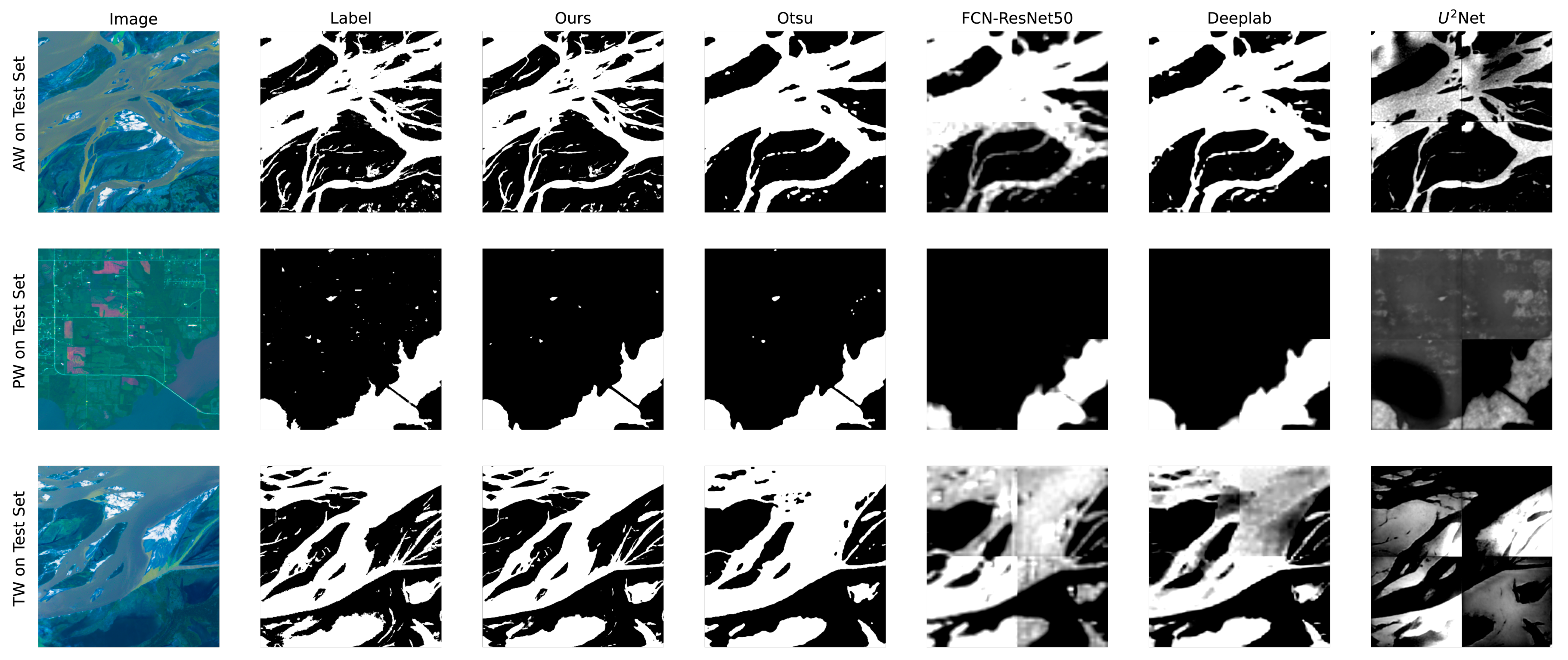
49] is designed to deal with the extreme imbalance between water/non-water, difficult/easy pixels during training. The ablation experimental results show the effectiveness of focal loss in dealing with a sample imbalance problem. Optical imagery contains information on the ground surface’s multispectral reflectivity, which is widely used in water indices and thresholding methods. Image fusion aims to use optical image data to assist SAR image prediction. Our experimental results demonstrate that optical imagery can provide useful supplementary information on water segmentation.
However, all water and temporary water have poor mIoU scores. There are two reasons to explain this phenomenon. One reason is the training process, as the image of all water and temporary water data have more water pixels and fewer non-water pixels. The difference in the sample size leads to differences in the learning effect. From OMISSION and COMMISSION, we can see that the all water and temporary water tasks perform better than permanent water on water pixels, and perform worse on non-water pixels. On the whole, non-water pixels dominate our data. The poorer prediction of non-water pixels leads to worse overall results. The other reason is the difference in image characteristics, and the images in all water and temporary water data contain more small tributaries and scattered areas from newly flooded areas. These areas are usually more challenging to identify.
With the help of hybrid loss, our model pays more attention to boundary pixels and increasing the confidence of the prediction. As a result, our method can not only produce richer details and sharper boundaries but also distinguish water and non-water pixels with a larger probability gap. The excellent feature extraction ability of deep learning model enables our model to deal with some challenging scenes.

6. Conclusions

In this paper, we developed an efficient model for detecting permanent water and temporary water in flood disasters by fusing Sentinel-1 and Sentinel-2 Imagery using a deep learning algorithm with the help of benchmark Sen1Floods11 datasets. The BASNet network adopted in this can capture both large-scale and detailed structural features. By combining with focal loss, our model achieved state-of-the-art accuracy for hard boundary pixels’ identification. The model’s performance was further improved by fusing the multi-source information, and the ablation study verified the effectiveness of each improvement measures. The comparison experiment results demonstrated that the implemented method could detect permanent water and temporary water flood more accurately than other methods. The proposed model performed well on the unknown Bolivia test set, which verifies its robustness. Due to the network architecture’s modularity, it can be easily adapted to data from other sensors. Finally, the method does not require prior knowledge, additional data pre-processing, and multi-temporal data, which significantly reduces the method’s complexity and increases the degree of automation.
Ongoing and future works focus on training water segmentation models on high spatial resolution remote sensing imagery. High spatial resolution remote sensing imagery has more complex background information, objects with larger-scale variation, and more unbalanced pixel classes [58]. More sophisticated modules are required to extract and fuse richer image information. In addition, the existing pre-trained neural networks are all based on RGB images, and, directly applied to remote sensing images, may reduce the efficiency of transfer learning due to differences in the data distribution. McKay et al. [61] dealt with this problem by discarding deep feature layers. Qin et al. [60] designed a network that allows for training from scratch, but this lighter network may degrade the performance. Although we dramatically improved the results of flood mapping, there is still much work to do.

Author Contributions

Conceptualization, Y.B.; methodology, Y.B. and H.Y.; software, W.W.; validation, W.W.; formal analysis, W.W.; investigation, Y.B. and H.Y.; resources, Y.B., H.Y., and Z.Y.; data curation, W.W.; writing—original draft preparation, Y.B. and W.W.; writing—review and editing, Y.B., W.W., J.Y., B.Z., X.L., E.M., and S.K.; visualization, W.W.; supervision, Y.B., J.Y., B.Z., X.L., E.M., and S.K.; project administration, Y.B.; funding acquisition, Y.B., H.Y., and Z.Y.; All authors have read and agreed to the published version of the manuscript.

Funding

This research was partly funded by the Fundamental Research Funds for the Central Universities, Research Funds of Renmin University of China (20XNF022), the fund for building world-class universities (disciplines) of Renmin University of China, the Japan Society for the Promotion of Science Kakenhi Program (17H06108), and Core Research Cluster of Disaster Science and Tough Cyberphysical AI Research Center at Tohoku University. The author gratefully acknowledges the support of K.C. Wong Education Foundation, Hong Kong.

Institutional Review Board Statement

Not applicable.

Informed Consent Statement

Not applicable.

Data Availability Statement

The Sen1Floods11 we utilized in this study can be reached at https://github.com/cloudtostreet/Sen1Floods11 (accessed on 10 November 2020).

Acknowledgments

This work was supported by the Public Computing Cloud, Renmin University of China. We also thank the Core Research Cluster of Disaster Science at Tohoku University (a Designated National University) for their support. We thank the reviewers for their helpful and constructive comments on our work. The author gratefully acknowledges the support of K.C. Wong Education Foundation, Hong Kong.

Conflicts of Interest

The authors declare no conflict of interest.

Abbreviations

The following abbreviations are used in this manuscript:
AWAll Water
BCEBinary Cross Entropy
CNNConvolutional Neural Network
COMMISSIONCommission Error Rates
DRDistributional Ranking
ESAEuropean Space Agency
FCNNFully Convolutional Neural Network
GEEGoogle Earth Engine
HANDHeight above Nearest Drainage
IoUIntersection over Union
JRCEuropean Commission Joint Research Centre
mIoUmean Intersection over Union
MNDWIModified Normalized Difference Water Index
NDFINormalized Difference Flood Index
NDFVINormalized Difference Flood in Vegetated Areas Index
NDVINormalized Difference Vegetation Index
OAOverall Accuracy
OMISSIONOmission Error Rates
PWPermanent Water
RAPIDRAdar-Produced Inundation Diary
ReLURectified Linear Unit
RRMResidual Refinement Module
SARSynthetic Aperture Radar
SODSalient Object Detection
SSIMStructural SIMilarity
TWTemporary Water
TOATop of Atmosphere

References

  1. IFRC. World Disaster Report 2020. Available online: https://media.ifrc.org/ifrc/world-disaster-report-2020/ (accessed on 18 January 2021).
  2. IDMC. Global Report on Internal Displacement. Available online: https://www.internal-displacement.org/sites/default/files/publications/documents/2019-IDMC-GRID.pdf (accessed on 17 January 2021).
  3. Aon. Weather, Climate & Catastrophe Insight 2019 Annual Report. Available online: http://thoughtleadership.aon.com/Documents/20200122-if-natcat2020.pdf?utm_source=ceros&utm_medium=storypage&utm_campaign=natcat20 (accessed on 18 January 2021).
  4. FAO. The State of Food Security and Nutrition in the World. Available online: http://www.fao.org/3/I9553EN/i9553en.pdf (accessed on 18 January 2021).
  5. Bonafilia, D.; Tellman, B.; Anderson, T.; Issenberg, E. Sen1Floods11: A Georeferenced Dataset to Train and Test Deep Learning Flood Algorithms for Sentinel-1. In Proceedings of the IEEE/CVF Conference on Computer Vision and Pattern Recognition Workshops, Seattle, WA, USA, 14–19 June 2020; pp. 210–211. [Google Scholar]
  6. Mason, D.C.; Speck, R.; Devereux, B.; Schumann, G.J.P.; Neal, J.C.; Bates, P.D. Flood Detection in Urban Areas Using TerraSAR-X. IEEE Trans. Geosci. Remote Sens. 2010, 48, 882–894. [Google Scholar] [CrossRef] [Green Version]
  7. Alfieri, L.; Cohen, S.; Galantowicz, J.; Schumann, G.J.; Trigg, M.A.; Zsoter, E.; Prudhomme, C.; Kruczkiewicz, A.; de Perez, E.C.; Flamig, Z.; et al. A global network for operational flood risk reduction. Environ. Sci. Policy 2018, 84, 149–158. [Google Scholar] [CrossRef]
  8. Zajic, B. How flood mapping from space protects the vulnerable and can save lives. Planet Labs 2019, 17. [Google Scholar]
  9. Oddo, P.C.; Bolten, J.D. The value of near real-time earth observations for improved flood disaster response. Front. Environ. Sci. 2019, 7, 127. [Google Scholar] [CrossRef] [Green Version]
  10. Enenkel, M.; Osgood, D.; Anderson, M.; Powell, B.; McCarty, J.; Neigh, C.; Carroll, M.; Wooten, M.; Husak, G.; Hain, C.; et al. Exploiting the convergence of evidence in satellite data for advanced weather index insurance design. Weather. Clim. Soc. 2019, 11, 65–93. [Google Scholar] [CrossRef]
  11. Okada, G.; Moya, L.; Mas, E.; Koshimura, S. The Potential Role of News Media to Construct a Machine Learning Based Damage Mapping Framework. Remote Sens. 2021, 13, 1401. [Google Scholar] [CrossRef]
  12. Martinis, S.; Twele, A.; Voigt, S. Towards operational near real-time flood detection using a split-based automatic thresholding procedure on high resolution TerraSAR-X data. Nat. Hazards Earth Syst. Sci. 2009, 9, 303–314. [Google Scholar] [CrossRef]
  13. Mahoney, C.; Merchant, M.; Boychuk, L.; Hopkinson, C.; Brisco, B. Automated SAR Image Thresholds for Water Mask Production in Alberta’s Boreal Region. Remote Sens. 2020, 12, 2223. [Google Scholar] [CrossRef]
  14. Tiwari, V.; Kumar, V.; Matin, M.A.; Thapa, A.; Ellenburg, W.L.; Gupta, N.; Thapa, S. Flood inundation mapping- Kerala 2018; Harnessing the power of SAR, automatic threshold detection method and Google Earth Engine. PLoS ONE 2020, 15, e0237324. [Google Scholar] [CrossRef]
  15. Otsu, N. Threshold selection method from gray-level histograms. IEEE Trans. Syst. Man Cybern. 1979, 9, 62–66. [Google Scholar] [CrossRef] [Green Version]
  16. Bioresita, F.; Puissant, A.; Stumpf, A.; Malet, J.P. Fusion of Sentinel-1 and Sentinel-2 image time series for permanent and temporary surface water mapping. Int. J. Remote Sens. 2019, 40, 9026–9049. [Google Scholar] [CrossRef]
  17. Conde, F.C.; Munoz, M.D. Flood Monitoring Based on the Study of Sentinel-1 SAR Images: The Ebro River Case Study. Water 2019, 11, 2454. [Google Scholar] [CrossRef] [Green Version]
  18. Huang, M.M.; Jin, S.G. Rapid Flood Mapping and Evaluation with a Supervised Classifier and Change Detection in Shouguang Using Sentinel-1 SAR and Sentinel-2 Optical Data. Remote Sens. 2020, 12, 2073. [Google Scholar] [CrossRef]
  19. Markert, K.N.; Chishtie, F.; Anderson, E.R.; Saah, D.; Griffin, R.E. On the merging of optical and SAR satellite imagery for surface water mapping applications. Results Phys. 2018, 9, 275–277. [Google Scholar] [CrossRef]
  20. Benoudjit, A.; Guida, R. A Novel Fully Automated Mapping of the Flood Extent on SAR Images Using a Supervised Classifier. Remote Sens. 2019, 11, 779. [Google Scholar] [CrossRef] [Green Version]
  21. DeVries, B.; Huang, C.Q.; Armston, J.; Huang, W.L.; Jones, J.W.; Lang, M.W. Rapid and robust monitoring of flood events using Sentinel-1 and Landsat data on the Google Earth Engine. Remote Sens. Environ. 2020, 240, 111664. [Google Scholar] [CrossRef]
  22. Rudner, T.G.; Rußwurm, M.; Fil, J.; Pelich, R.; Bischke, B.; Kopačková, V.; Biliński, P. Multi3Net: Segmenting flooded buildings via fusion of multiresolution, multisensor, and multitemporal satellite imagery. In Proceedings of the AAAI Conference on Artificial Intelligence, Honolulu, HI, USA, 27 January–1 February 2019; Volume 33, pp. 702–709. [Google Scholar]
  23. Schlaffer, S.; Matgen, P.; Hollaus, M.; Wagner, W. Flood detection from multi-temporal SAR data using harmonic analysis and change detection. Int. J. Appl. Earth Obs. Geoinf. 2015, 38, 15–24. [Google Scholar] [CrossRef]
  24. Twele, A.; Cao, W.X.; Plank, S.; Martinis, S. Sentinel-1-based flood mapping: A fully automated processing chain. Int. J. Remote Sens. 2016, 37, 2990–3004. [Google Scholar] [CrossRef]
  25. Schlaffer, S.; Chini, M.; Giustarini, L.; Matgen, P. Probabilistic mapping of flood-induced backscatter changes in SAR time series. Int. J. Appl. Earth Obs. Geoinf. 2017, 56, 77–87. [Google Scholar] [CrossRef]
  26. Amitrano, D.; Di Martino, G.; Iodice, A.; Riccio, D.; Ruello, G. Unsupervised Rapid Flood Mapping Using Sentinel-1 GRD SAR Images. IEEE Trans. Geosci. Remote Sens. 2018, 56, 3290–3299. [Google Scholar] [CrossRef]
  27. Moya, L.; Endo, Y.; Okada, G.; Koshimura, S.; Mas, E. Drawback in the change detection approach: False detection during the 2018 western Japan floods. Remote Sens. 2019, 11, 2320. [Google Scholar] [CrossRef] [Green Version]
  28. Moya, L.; Mas, E.; Koshimura, S. Learning from the 2018 Western Japan Heavy Rains to Detect Floods during the 2019 Hagibis Typhoon. Remote Sens. 2020, 12, 2244. [Google Scholar] [CrossRef]
  29. Bai, Y.; Gao, C.; Singh, S.; Koch, M.; Adriano, B.; Mas, E.; Koshimura, S. A framework of rapid regional tsunami damage recognition from post-event TerraSAR-X imagery using deep neural networks. IEEE Geosci. Remote Sens. Lett. 2017, 15, 43–47. [Google Scholar] [CrossRef] [Green Version]
  30. Bai, Y.; Mas, E.; Koshimura, S. Towards operational satellite-based damage-mapping using u-net convolutional network: A case study of 2011 tohoku earthquake-tsunami. Remote Sens. 2018, 10, 1626. [Google Scholar] [CrossRef] [Green Version]
  31. Kang, W.; Xiang, Y.; Wang, F.; Wan, L.; You, H. Flood detection in gaofen-3 SAR images via fully convolutional networks. Sensors 2018, 18, 2915. [Google Scholar] [CrossRef] [Green Version]
  32. Li, Y.; Martinis, S.; Wieland, M. Urban flood mapping with an active self-learning convolutional neural network based on TerraSAR-X intensity and interferometric coherence. ISPRS J. Photogramm. Remote Sens. 2019, 152, 178–191. [Google Scholar] [CrossRef]
  33. Chen, L.; Zhang, P.; Xing, J.; Li, Z.; Xing, X.; Yuan, Z. A Multi-Scale Deep Neural Network for Water Detection from SAR Images in the Mountainous Areas. Remote Sens. 2020, 12, 3205. [Google Scholar] [CrossRef]
  34. Wangchuk, S.; Bolch, T. Mapping of glacial lakes using Sentinel-1 and Sentinel-2 data and a random forest classifier: Strengths and challenges. Sci. Remote Sens. 2020, 2, 100008. [Google Scholar] [CrossRef]
  35. Zhang, Y.; Zhang, G.; Zhu, T. Seasonal cycles of lakes on the Tibetan Plateau detected by Sentinel-1 SAR data. Sci. Total Environ. 2020, 703, 135563. [Google Scholar] [CrossRef]
  36. Sunkara, V.; Purri, M.; Saux, B.L.; Adams, J. Street to Cloud: Improving Flood Maps With Crowdsourcing and Semantic Segmentation. arXiv 2020, arXiv:2011.08010. [Google Scholar]
  37. Muñoz, D.F.; Muñoz, P.; Moftakhari, H.; Moradkhani, H. From Local to Regional Compound Flood Mapping with Deep Learning and Data Fusion Techniques. Sci. Total Environ. 2021, 146927. [Google Scholar] [CrossRef]
  38. Bai, Y.; Hu, J.; Su, J.; Liu, X.; Liu, H.; He, X.; Meng, S.; Mas, E.; Koshimura, S. Pyramid Pooling Module-Based Semi-Siamese Network: A Benchmark Model for Assessing Building Damage from xBD Satellite Imagery Datasets. Remote Sens. 2020, 12, 4055. [Google Scholar] [CrossRef]
  39. Su, J.; Bai, Y.; Wang, X.; Lu, D.; Zhao, B.; Yang, H.; Mas, E.; Koshimura, S. Technical Solution Discussion for Key Challenges of Operational Convolutional Neural Network-Based Building-Damage Assessment from Satellite Imagery: Perspective from Benchmark xBD Dataset. Remote Sens. 2020, 12, 3808. [Google Scholar] [CrossRef]
  40. FloodNet: A High Resolution Aerial Imagery Dataset for Post Flood Scene Understanding. arXiv 2020, arXiv:2012.02951.
  41. Konapala, G.; Kumar, S. Exploring Sentinel-1 and Sentinel-2 Diversity for Flood Inundation Mapping Using Deep Learning. Technical Report. Copernicus Meetings. 2021. Available online: https://0-doi-org.brum.beds.ac.uk/10.5194/egusphere-egu21-10445 (accessed on 4 March 2021).
  42. Li, Y.; Martinis, S.; Plank, S.; Ludwig, R. An automatic change detection approach for rapid flood mapping in Sentinel-1 SAR data. Int. J. Appl. Earth Obs. Geoinf. 2018, 73, 123–135. [Google Scholar] [CrossRef]
  43. Qin, X.; Zhang, Z.; Huang, C.; Gao, C.; Dehghan, M.; Jagersand, M. Basnet: Boundary-aware salient object detection. In Proceedings of the IEEE Conference on Computer Vision and Pattern Recognition, Long Beach, CA, USA, 15–20 June 2019; pp. 7479–7489. [Google Scholar]
  44. Ioffe, S.; Szegedy, C. Batch normalization: Accelerating deep network training by reducing internal covariate shift. arXiv 2015, arXiv:1502.03167. [Google Scholar]
  45. Hahnloser, R.H.; Seung, H.S.; Slotine, J.J. Permitted and forbidden sets in symmetric threshold-linear networks. Neural Comput. 2003, 15, 621–638. [Google Scholar] [CrossRef] [PubMed]
  46. He, K.; Zhang, X.; Ren, S.; Sun, J. Deep residual learning for image recognition. In Proceedings of the IEEE Conference on Computer Vision and Pattern Recognition, Las Vegas, NV, USA, 26 June–1 July 2016; pp. 770–778. [Google Scholar]
  47. Chen, L.C.; Papandreou, G.; Kokkinos, I.; Murphy, K.; Yuille, A.L. Semantic image segmentation with deep convolutional nets and fully connected crfs. arXiv 2014, arXiv:1412.7062. [Google Scholar]
  48. Chen, L.C.; Papandreou, G.; Kokkinos, I.; Murphy, K.; Yuille, A.L. Deeplab: Semantic image segmentation with deep convolutional nets, atrous convolution, and fully connected crfs. IEEE Trans. Pattern Anal. Intell. Mach. 2017, 40, 834–848. [Google Scholar] [CrossRef]
  49. Goyal, P.; Kaiming, H. Focal loss for dense object detection. In Proceedings of the IEEE International Conference on Computer Vision, Venice, Italy, 22–29 October 2017; pp. 2980–2988. [Google Scholar]
  50. Wang, Z.; Simoncelli, E.P.; Bovik, A.C. Multiscale structural similarity for image quality assessment. In Proceedings of the The Thrity-Seventh Asilomar Conference on Signals, Systems & Computers, Pacific Grove, CA, USA, 9–12 November 2003; Volume 2, pp. 1398–1402. [Google Scholar]
  51. Máttyus, G.; Luo, W.; Urtasun, R. Deeproadmapper: Extracting road topology from aerial images. In Proceedings of the IEEE International Conference on Computer Vision, Venice, Italy, 22–29 October 2017; pp. 3438–3446. [Google Scholar]
  52. Deng, J.; Dong, W.; Socher, R.; Li, L.J.; Li, K.; Fei-Fei, L. Imagenet: A large-scale hierarchical image database. In Proceedings of the 2009 IEEE Conference on Computer Vision and Pattern Recognition, Miami, FL, USA, 20–25 June 2009; pp. 248–255. [Google Scholar]
  53. Glorot, X.; Bengio, Y. Understanding the difficulty of training deep feedforward neural networks. In Proceedings of the Thirteenth International Conference on Artificial Intelligence and Statistics, Sardinia, Italy, 13–15 May 2010; pp. 249–256. [Google Scholar]
  54. Kingma, D.P.; Ba, J. Adam: A method for stochastic optimization. arXiv 2014, arXiv:1412.6980. [Google Scholar]
  55. Banko, G. A Review of Assessing the Accuracy of Classifications of Remotely Sensed Data and of Methods Including Remote Sensing Data in Forest Inventory; International Institute for Applied Systems Analysis: Laxenburg, Austria, 1998. [Google Scholar]
  56. Chang, C.H.; Lee, H.; Kim, D.; Hwang, E.; Hossain, F.; Chishtie, F.; Jayasinghe, S.; Basnayake, S. Hindcast and forecast of daily inundation extents using satellite SAR and altimetry data with rotated empirical orthogonal function analysis: Case study in Tonle Sap Lake Floodplain. Remote Sens. Environ. 2020, 241, 111732. [Google Scholar] [CrossRef]
  57. Qian, Q.; Chen, L.; Li, H.; Jin, R. DR loss: Improving object detection by distributional ranking. In Proceedings of the IEEE/CVF Conference on Computer Vision and Pattern Recognition, Seattle, WA, USA, 14–19 June 2020; pp. 12164–12172. [Google Scholar]
  58. Zheng, Z.; Zhong, Y.; Wang, J.; Ma, A. Foreground-Aware Relation Network for Geospatial Object Segmentation in High Spatial Resolution Remote Sensing Imagery. In Proceedings of the IEEE/CVF Conference on Computer Vision and Pattern Recognition, Seattle, WA, USA, 14–19 June 2020; pp. 4096–4105. [Google Scholar]
  59. Chen, L.C.; Zhu, Y.; Papandreou, G.; Schroff, F.; Adam, H. Encoder-decoder with atrous separable convolution for semantic image segmentation. In Proceedings of the European conference on computer vision (ECCV), Munich, Germany, 8–14 September 2018; pp. 801–818. [Google Scholar]
  60. Qin, X.; Zhang, Z.; Huang, C.; Dehghan, M.; Zaiane, O.R.; Jagersand, M. U2-Net: Going deeper with nested U-structure for salient object detection. Pattern Recognit. 2020, 106, 107404. [Google Scholar] [CrossRef]
  61. McKay, J.; Gag, I.; Monga, V.; Raj, R.G.; Ieee. What’s Mine is Yours: Pretrained CNNs for Limited Training Sonar ATR. arXiv 2017, arXiv:1706.09858. [Google Scholar]
Figure 1. Sample locations of flood event data.
Remotesensing 13 02220 g001
Figure 2. Example of all the bands.
Remotesensing 13 02220 g002
Figure 3. Illustration of water label. (a) example of hand labeled data of all water; (b) example of hand labeled data of permanent water; (c) the illustration of temporary water, permanent water, and all water.
Remotesensing 13 02220 g003
Figure 4. Flowchart of water type detection proposed in this work.
Remotesensing 13 02220 g004
Figure 5. Architecture of the BASNet used in this study.
Remotesensing 13 02220 g005
Figure 6. Qualitative comparison of proposed method with other methods. Each row represents one image and corresponding flooding maps (binary maps for the Otsu method, probability maps for FCN-ResNet50, Deeplab, U 2 Net, and our model). Each column represents one method. Results shown on all water (AW), permanent water (PW), and temporary water (TW).
Remotesensing 13 02220 g006
Figure 7. Qualitative comparison of proposed method with other methods. Each row represents one image and corresponding flooding maps (binary maps for the Otsu method, probability maps for FCN-ResNet50, Deeplab, U 2 Net, and our model). Each column represents one method. Results shown on all water (AW), permanent water (PW), and temporary water (TW).
Remotesensing 13 02220 g007
Table 1. Water, Non-Water, and Ignored area proportion in pixel level
LabelWaterNon-WaterIgnored
All Water9.16%77.22%13.63%
Permanent Water3.06%96.94%0.00%
Table 2. Sen1Floods11 dataset composition
DatasetSample Size
Training SetHand-Labeled252
Weakly-Labeled4160
Validation Set89
Testing Set90
Bolivia Testing Set15
Table 3. Evaluation on the Sen1Floods11 test set for ablation studies. Results showed on all water (AW), permanent water (PW), and temporary water (TW).
TaskMethodAugmentsFocal LossImage FusemloU (%)IoU (%)OA (%)
All WaterBaseline 29.3935.0879.49
+Augments 30.3642.2784.04
+Focal Loss 42.7754.1090.58
+Image Fuse 47.6063.1392.85
+Augments+Focal Loss 42.9553.8690.80
+Augments+Focal Loss+Image Fuse58.7364.5293.38
Permanent WaterBaseline 40.0945.8191.50
+Augments 34.1038.1488.18
+Focal Loss 50.0635.4891.47
+Image Fuse 65.0450.8193.49
+Augments+Focal Loss 59.7450.8893.50
+Augments+Focal Loss+Image Fuse68.7952.0393.84
Temporary WaterBaseline 25.6931.6883.52
+Augments 27.8133.4485.60
+Focal Loss 34.6439.1989.13
+Image Fuse 50.5351.1992.97
+Augments+Focal Loss 34.7538.9988.19
+Augments+Focal Loss+Image Fuse52.9952.3092.81
Table 4. Evaluation on Sen1Floods11 Bolivia test set for ablation studies. Results shown on all water (AW), permanent water (PW), and temporary water (TW).
TaskMethodAugmentsFocal LossImage FusemloU (%)IoU (%)OA (%)
All WaterBaseline 45.3164.5491.40
+Augments 45.5164.9591.53
+Focal Loss 47.1270.6394.07
+Image Fuse 46.3967.3792.22
+Augments+Focal Loss 47.4271.2394.20
+Augments+Focal Loss+Image Fuse54.0778.9095.79
Permanent WaterBaseline 38.7836.1095.31
+Augments 43.3740.4394.32
+Focal Loss 67.2971.7999.06
+Image Fuse 72.3075.4299.23
+Augments+Focal Loss 70.2376.4599.22
+Augments+Focal Loss+Image Fuse75.2778.8099.39
Temporary WaterBaseline 40.6964.3291.76
+Augments 40.7064.6692.08
+Focal Loss 41.1266.4792.79
+Image Fuse 43.5370.6094.23
+Augments+Focal Loss 40.6564.1392.20
+Augments+Focal Loss+Image Fuse47.8876.7495.59
Table 5. Water, Non-Water, and Ignored area proportion at the pixel level of all water (AW), permanent water (PW), and temporary water (TW).
LabelWaterNon-WaterIgnored
All Water9.16%77.22%13.63%
Permanent Water4.26%74.49%21.25%
Temporary Water6.54%77.22%16.25%
Table 6. Comparison on different losses in terms of mIoU(%) on the Sen1Floods11 test set. Results shown on all water (AW), permanent water (PW), and temporary water (TW).
LossAWPWTW
Normalized Focal Loss42.2657.0035.23
DR Loss43.3258.0536.87
Focal Loss42.9559.7434.75
Table 7. Comparison on different losses in terms of mIoU(%) on the Sen1Floods11 Bolivia test set. Results shown on all water (AW), permanent water (PW), and temporary water (TW).
LossAWPWTW
Normalized Focal Loss47.3667.0840.33
DR Loss43.9959.4136.08
Focal Loss47.4270.2440.65
Table 8. Performance comparison with other methods on Sen1Floods11 test set. Results shown on all water (AW), permanent water (PW), and temporary water (TW). xx indicates the best performance.
TaskMethodmIoU(%)IoU(%)OMISSION(%)COMMISSION(%)OA(%)
All WaterOtsu35.7354.5826.684.9190.01
FCN-ResNet5030.949.3228.498.2688.56
Deeplab v332.0847.6734.896.7287.96
U 2 Net38.3952.0332.955.3089.96
BASNet58.7364.5231.191.1693.38
Permanent WaterOtsu47.7862.811.224.9092.83
FCN-ResNet5035.1955.1118.047.5590.70
Deeplab v337.5444.6043.554.1290.18
U 2 Net38.3627.8064.034.5688.34
BASNet68.7952.0347.430.1693.84
Temporary WaterOtsu27.9538.9840.424.9189.13
FCN-ResNet5022.5530.3024.4919.9379.50
Deeplab v334.4941.5846.093.9690.27
U 2 Net31.0544.0836.076.0189.77
BASNet52.9952.3043.151.1692.81
Table 9. Performance comparison with other methods on Bolivia datasets. Results shown on all water (AW), permanent water (PW), and temporary water (TW). xx indicates the best performance.
TaskMethodmIoU(%)IoU(%)OMISSION(%)COMMISSION(%)OA(%)
All WaterOtsu48.2270.5812.854.5893.64
FCN-ResNet5043.5257.3210.1910.6889.53
Deeplab v344.4668.1110.285.9892.89
U 2 Net40.1156.609.1011.4388.53
BASNet54.0778.907.663.2195.79
Permanent WaterOtsu36.2635.2055.365.2593.47
FCN-ResNet5032.9822.6416.608.3791.43
Deeplab v336.0934.5011.834.8693.08
U 2 Net40.1334.0620.124.2095.55
BASNet75.2778.8018.600.1099.39
Temporary WaterOtsu42.2369.2813.354.5893.64
FCN-ResNet5036.2138.7210.4823.1078.74
Deeplab v331.4054.7429.774.9890.80
U 2 Net35.2953.067.4713.1087.60
BASNet47.8876.749.853.0895.59
Publisher’s Note: MDPI stays neutral with regard to jurisdictional claims in published maps and institutional affiliations.

