
Squint Model InISAR Imaging Method Based on Reference Interferometric Phase Construction and Coordinate Transformation


1
Key Laboratory of Microwave Remote Sensing, Chinese Academy of Sciences, Beijing 100190, China
2
National Space Science Center, Chinese Academy of Sciences, Beijing 100190, China
3
School of Electronic, Electrical and Communication Engineering, University of Chinese Academy of Sciences, Beijing 100049, China
*
Author to whom correspondence should be addressed.
Remote Sens. 2021, 13(11), 2224; https://0-doi-org.brum.beds.ac.uk/10.3390/rs13112224
Submission received: 1 April 2021
/
Accepted: 4 June 2021
/
Published: 7 June 2021
Abstract
:The imaging quality of InISAR under squint geometry can be greatly degraded due to the serious interferometric phase ambiguity (InPhaA) and thus result in image distortion problems. Aiming to solve these problems, a three-dimensional InISAR (3D ISAR) imaging method based on reference InPhas construction and coordinate transformation is presented in this paper. First, the target’s 3D coarse location is obtained by the cross-correlation algorithm, and a relatively stronger scatterer is taken as the reference scatterer to construct the reference interferometric phases (InPhas) so as to remove the InPhaA and restore the real InPhas. The selected scatterer needs not to be exactly in the center of the coarsely located target. Then, the image distortion is corrected by coordinate transformation, and finally the 3D coordinates of the target can be accurately estimated. Both simulation and practical experiment results validate the effectiveness of the method.
1. Introduction
Inverse synthetic aperture radar (ISAR) can perform two-dimensional imaging of non-cooperative targets at all-time and in all-weather conditions [1,2,3,4]. However, some problems exist in ISAR preventing its further application. First, the ISAR image usually exhibits the Doppler frequency distribution of the target in the cross-range direction rather than the cross-range scale of target. Typically, it is very difficult to get prior motion information including rotation data about a non-cooperative target, and thus its cross-range scale cannot be easily obtained [5,6]. Second, ISAR imaging is a projective mapping of the target on the range-Doppler plane that is called the image plane. When the target has complex motions, the image plane is usually uncertain, and the real structure and size of the imaged target cannot be easily recognized and calculated [6]. These problems can be solved by interferometric inverse synthetic aperture radar (InISAR) because three-dimensional imaging of the target can be directly obtained without concerning the imaging plane as well as the cross-range scaling [6,7,8,9,10,11,12,13].
InISAR realizes 3D imaging by using several antennas arranged in a specific way to form two orthogonal baselines to obtain the interferometric phases (InPhas) which are used to retrieve the 3D structure of the imaged target [14,15,16,17,18,19]. Accurate estimation of InPha is the key issue for InISAR. However, the directly measured InPhas usually suffer from an ambiguity problem because any InPha larger than 2π will be wrapped into (0, 2π) or (−π, π). In InISAR, the interferometric phase ambiguity (InPhaA) can be divided into two categories according to the causes. One is caused by phase wrapping resulting from a large target size, long distance of target, and long baseline as well as short radar wavelength [20]. The another is caused by the squint effect induced when the target is largely deviated from the normal directions of the baselines [21], and this InPhaA is similar to that induced by the flat-earth effect in InSAR. The squint effect introduces an additional InPha, i.e., the squint phase, which results in InPhaA, and thus affects the subsequent phase unwrapping and 3D target reconstruction. Therefore, if the imaging system is under the squint model, the squint effect must be removed before phase unwrapping and 3D target reconstruction. In this paper, we focus on solving the InPhaA problem caused by the squint effect.
In a general InISAR system, it is assumed that the target is located near the antenna axis, i.e., the normal model can be adopted. But in practical applications, the target is usually far away from the antenna axis, i.e., the squint model should be adopted [21,22,23,24]. For convenience, we denote the perpendicular bisector of the baseline as the antenna axis [25]. Although any single antenna can be rotated mechanically, it is difficult to rotate the baselines to make the target lie in the antenna axis as defined above because it means that we should move the antennas simultaneously [22]. In [23], the path integration method was applied to unwrapping the ambiguous InPhas. However, the obtained ISAR image of target usually exhibits as discrete scattering centers, that is to say, the distribution of the InPhas is not continuous, so the path integration method is not completely applicable to InISAR. In [22], an isolated scatterer on the ISAR image is used as a reference scatterer to remove the InPhaA of other scatterers, but the phase error of this reference on different ISAR images will affect the interferometric phase compensation. At the same time, a lot of approximations are used in the 3D coordinates estimation of the target, which undoubtedly reduces the accuracy of the coordinates estimation. In [24], an imaging method was proposed based on the known target center or accurate 3D location of the target. The nonlinear equations used to estimate the scatterer coordinates with this method are very complicated and must be solved for every scatterer through an iterative approach; therefore, the computation load is very large. In [25], the method for the InPhaA removal is the same as that in [24], but the iterative method in coordinates estimation has been improved to promote the computational efficiency. In [26], in order to remove the InPhaA, the InPha of each scatterer from the ISAR image pair is extracted to estimate the fuzzy factor. However, this method may not work when multiple scatterers are contained in each range-Doppler cell.
This paper presents a 3D squint model InISAR imaging method based on a L-shape cost-effective three-antenna configuration. The method includes two key operations, i.e., the reference InPhas construction and the coordinate transformation. Compared with [25], there are two essential advantages: (1) the reference InPhas are constructed by roughly determining a reference scatterer to remove the InPhA instead of dechirping the echoes of different channels separately by taking the echoes of the target center as the reference echoes. Therefore, our method does not need to accurately know the coordinates of the ISAR images’ centers, but this is not true for the method in [25]; (2) 3D coordinates of scatterers are directly estimated without iteration, so the proposed method has less computation effort compared with that by iteration.
We should point out that the motion error compensation (MEC) is very important for better ISAR imaging. However, for the squint InISAR, we do not need to treat the MEC as a special problem different from that for ISAR because for each single antenna of an InISAR system, the target should be tracked and maintained around the boresight to guarantee enough signal to noise ratio (SNR). Therefore, the MEC is not especially concerned in this work.
The remainder of the paper is arranged as follows. The basic principle of 3D InISAR imaging under the normal model and the influence of the squint effect are briefly described in Section 2. The new InISAR imaging method is detailed in Section 3. Simulation and experiment results are respectively presented in Section 4 and Section 5, and finally Section 6 concludes the paper.
2. Principle of 3D InISAR Imaging
2.1. Normal Model
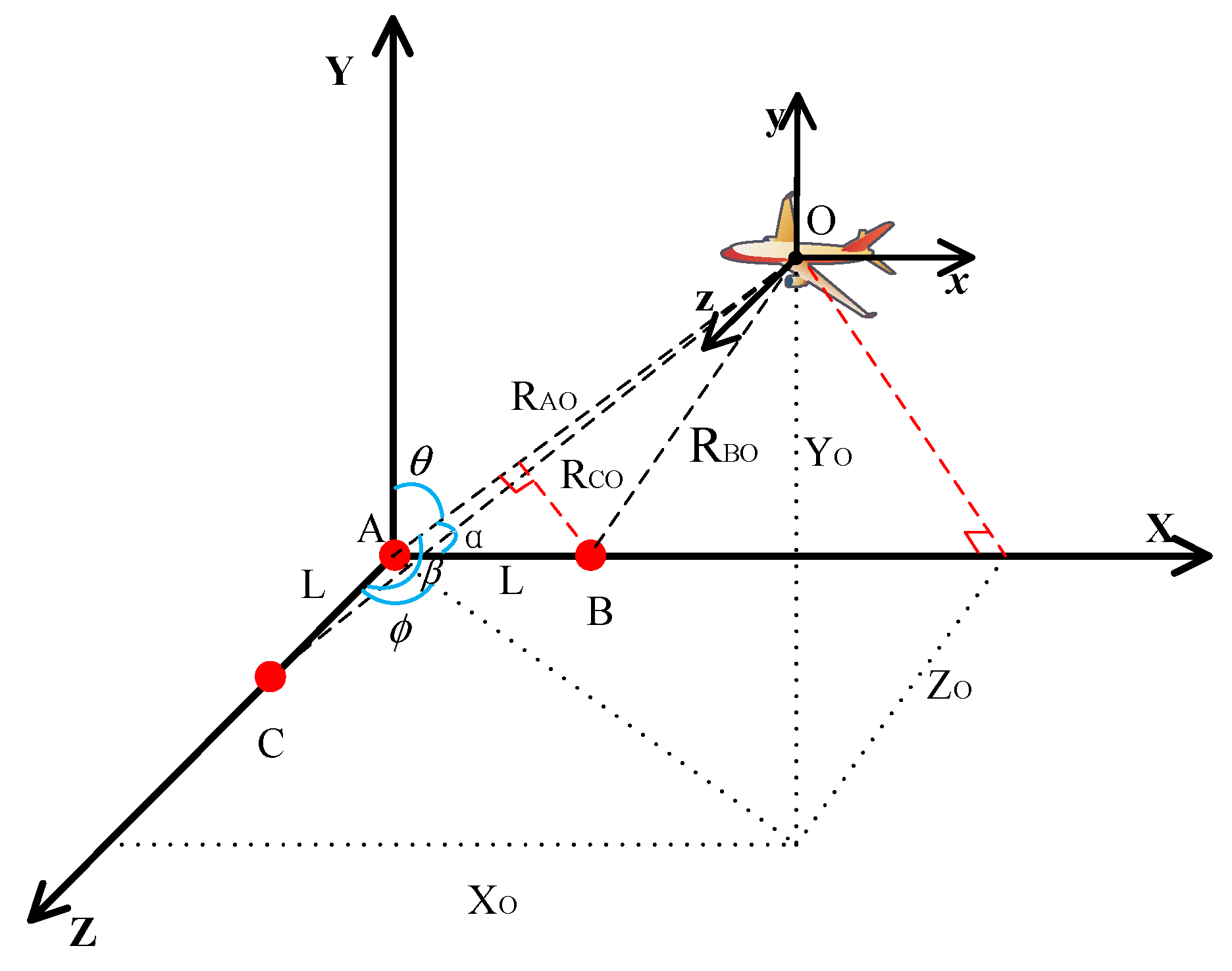
InISAR realizes 3D imaging of long-distance moving targets by exploring the InPhas generated from three or more ISAR images obtained by multiple antennas forming orthogonal baselines, which can achieve the cross-range scaling of the target without estimation of the rotation velocity. For convenience, we use the simplest and cost-effective 3D InISAR system, i.e., an L-shaped three-antenna InISAR configuration [14], to study the squint effect. Figure 1 shows the InISAR geometry composed of three antennas located at A, B, and C, respectively, where α, θ, and β denote the angles between the line-of-sight (LOS) and the three axes X, Y, and Z, respectively. We used antenna A for both transmitting and receiving, while B and C were only used for receiving. In this model, the InISAR coordinate system is denoted by (X, Y, Z) with A taken as the origin, while the target coordinate system is denoted by (x, y, z) with O taken as the origin. Let us assume O(X0, Y0, Z0) is the initial location of the target center, and P(xp, yp, zp) is one of the scattering centers of the target. The initial distances between antennas A, B, C, and P are denoted as RAP0, RBP0, RCP0, respectively.
The radar transmits LFM pulses, which can be expressed as,
where t and tm are the fast and slow times, f0 is the carrier frequency, γ is the frequency-modulation rate, and TP is the time width of the transmitted pulse. Then, the echo from a single scatterer P can be expressed as,
where K represents different antennas, K∈{A, B, C}, ρK represents the scattering intensity of scatterer P received by antenna K, and τK(tm) is the echo delay relative to antenna K which can be expressed as,
where RKP(tm) represents the instantaneous distance from P to the radar K. During the short imaging time, the RKP(tm) can be treated as linearly varied, that is, RKP(tm) = RKP0 + VKPtm. After the pulse compression, motion compensation, and ISAR imaging processing, the ISAR image of each antenna can be expressed as,
where Tm denotes the imaging time, fm denotes the Doppler frequency, and λ denotes the wavelength of the carrier frequency of the transmitted signal. We should stress that if the aspect angle range (AAR) of observation is small, i.e., less than 1–2 degrees, Equation (4) can be obtained easily by azimuthal FFT after range compression. If the AAR is larger than several degrees and in a high-range resolution situation, then the 2D interpolation is required, i.e., Equation (4) can be obtained after complex interpolation processing, which is out of the scope of this paper.
After image registration, the InPhas can be obtained as,
where ΔRAB and ΔRAC represent the wave path differences between antennas A and B and between A and C, respectively. According to the imaging geometry of Figure 1, ΔRAB and ΔRAC can be estimated by,
Hence, Equations (5) and (6) can be respectively expressed as,
It is apparent that the real InPha of a scatterer between two antennas is proportional to the scatterer coordinate (i.e., XP ZP) along the baselines. However, the real InPha may be wrapped due to the measured InPha being unable to exceed (−π, π) and thus it suffers from InPhA. In other words, only when XP, ZP are small enough to meet the following conditions, can InPhaA can be avoided.
where XP and ZP are all determined by two parts, i.e., XP = XO + xp and ZP = ZO + zp, where XO and ZO respectively represent the X and Y coordinates of the origin of the target coordinate system in the coordinate system of InISAR, as introduced above, and xp and zp depend on the target size. As previously mentioned, the InPhaA caused by XO is called the squint effect which is focused on in this research. For the convenience of derivation, we temporarily ignore the InPhaA caused by xp, that is, we assume there is no InPhaA when XO = 0.
Under the normal model, XO is so small that XP is within the constraints of Equation (10) so XP can be directly estimated by
Meanwhile, YP can be approximated by the LOS range RAP.
In the same fashion, the 3D coordinates of the all scatterers can be estimated one by one, and thus the 3D imaging of the target is realized.
2.2. Squint Model
The antenna pair of A and B are taken as an example to explain the influence of the squint effect. The InPha φAB in Equation (8) can be rewritten as,
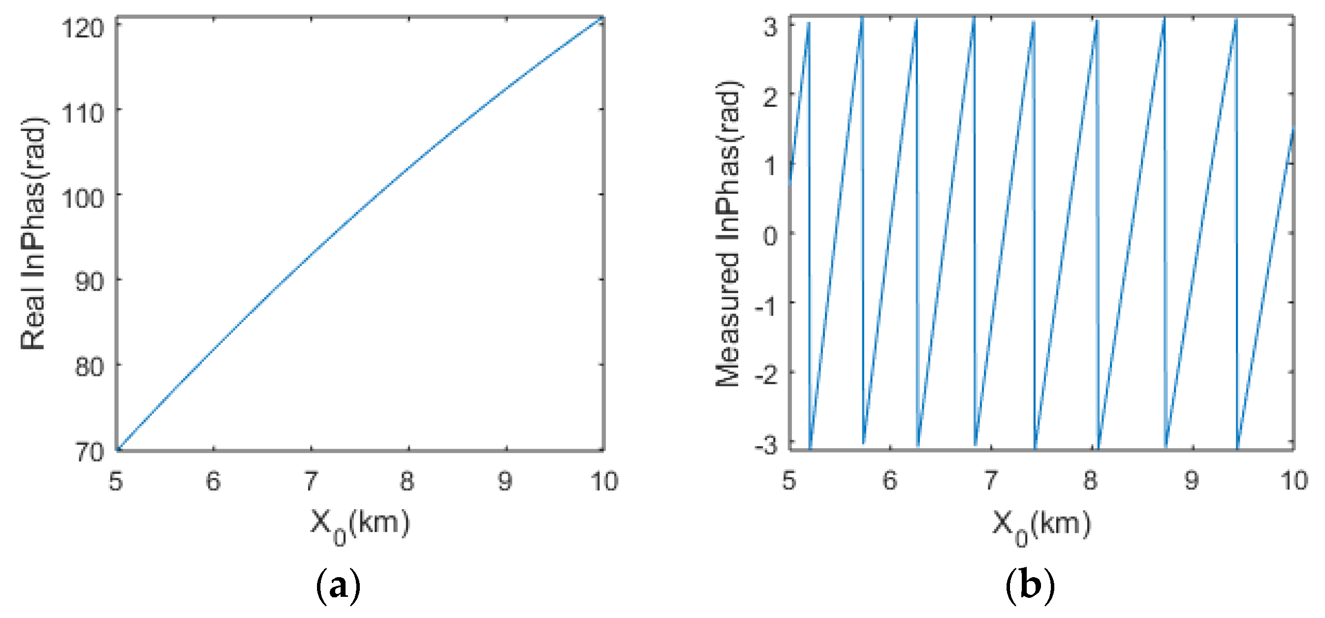
The InPha φAB is not only a function of xp, but also a function of XO as well, even if xp = 0, φAB will also change along with the variation of XO. Figure 2 demonstrates the influence of the squint effect on the InPha with YO = 10 km, ZO = 0, λ = 0.03 m, and L = 3 m assumed, where Figure 2a shows the real InPhas variation as XO changes from 5 km to 10 km, while Figure 2b shows the measured InPhas variation, which is wrapped. As a result, the measured InPhas will not satisfy Equation (10), which results in difficulties for subsequent InPha unwrapping and 3D target reconstruction.
In addition, as can be seen from Figure 1, the slant-range coordinate RAP of the ISAR image is not consistent with the Y-coordinate of the actual target under the squint model. If it is directly used for 3D reconstruction, distortion will be introduced, however, it can be corrected through coordinate transformation as addressed later in Section 3.2.
Therefore, in order to achieve high quality 3D InISAR imaging, we should eliminate the InPhaA and correct the image distortion caused by the squint effect.
3. InISAR Imaging Based on Reference InPhas Construction
As can be seen from Equation (13), the “①” term can be directly eliminated or at least greatly reduced to within the unambiguity range if the target center or a scatterer on the target is known. This is similar to the removal operation of the flat-earth effect in InSAR signal processing, where a horizontal plane of certain height is selected as the reference plane under the observation geometry. Then, the reference InPhas are constructed and used to remove the InPhaA. Compared with the removal of the flat-earth effect in InSAR, there are two key difficulties in the removal of the squint effect in InISAR. The first issue is how to select the reference scatterer due to the target being non-cooperative, and the second is how to correct the image distortion. The proposed method is motivated by solving these two difficulties and mainly includes the following three steps: reference InPhas construction; InPhas restoration; and 3D coordinate estimation, as shall be detailed in the following.
3.1. Reference InPhas Construction
According to Equation (7), the coordinates of an arbitrarily selected scattering point Q on the target can be coarsely estimated by Equation (14) with L << RAQ assumed,
where RAQ can be directly obtained by measuring the echo delay, ΔRAB and ΔRAC represent the wave path differences between antennas A and B and between A and C, respectively, which can be obtained by calculating the cross-correlation function (CCF) between two ISAR images of different channels as follows,
Then, the locations of the peak value of the CCFs can be obtained by,
Finally, the range bin shifts between different ISAR images can be calculated by,
where N is the sampling number, Δr is the range resolution. The results obtained by Equation (17) are also used for following image registration.
The coarse location of Q(XQ, YQ, ZQ) can be calculated by substituting RAQ, ΔRAB, and ΔRAC into Equation (14), and then Q (XQ, YQ, ZQ) is taken as the reference scatterer used to construct the reference InPhas by,
where RAQ, RBQ, and RCQ are the radial distances from the reference scatterer Q to the antennas A, B, and C, respectively.
It should be noted that although the proposed method does not require particularly high accuracy regarding the target location, it still has certain requirements on the location errors. We denote ΔX, ΔY, and ΔZ as the coordinate differences between the reference scatterer and the target center in the X, Y, Z directions, respectively. In order to ensure the InPhaA caused by the squint effect can be removed, the additional InPha introduced by ΔX, ΔY, and ΔZ cannot exceed (−π, π), so ΔX and ΔZ must meet the following limits,
3.2. InPhas Restoration
Based on the constructed reference InPhas, the InPhaA can be removed by,
where,
Since RAP − RBP − (RAQ − RBQ) and RAP − RCP − (RAQ − RCQ) can be very small, φAB_focus and φAC_focus will not exceed (−π, π), i.e., the InPhA is eliminated. Then, in order to make the InPha correctly reflect the echo difference between two antennas, we must restore the real InPhas by,
3.3. 3D Coordinates Estimation
Based on the recovered real InPhas, the x-coordinates and z-coordinates of scatterers in the target coordinate system with Q as the origin can be estimated by,
The above Equation (24) is derived from Equations (8) and (9), where XP = XO + xp and ZP = ZO + zp, here XO and ZO are replaced by XQ and ZQ.
It should be noted that the real InPhas (i.e., φAB_real and φAC_freal) can be very large in the far-field case, so RAP, RBP, and RCP in Equation (24) can no longer be approximated by RAO as the imaging method under the normal model does. Therefore, in order to guarantee the estimation accuracy, the LOS ranges of all scatterers are directly obtained by the echo delays of different receiving antennas.
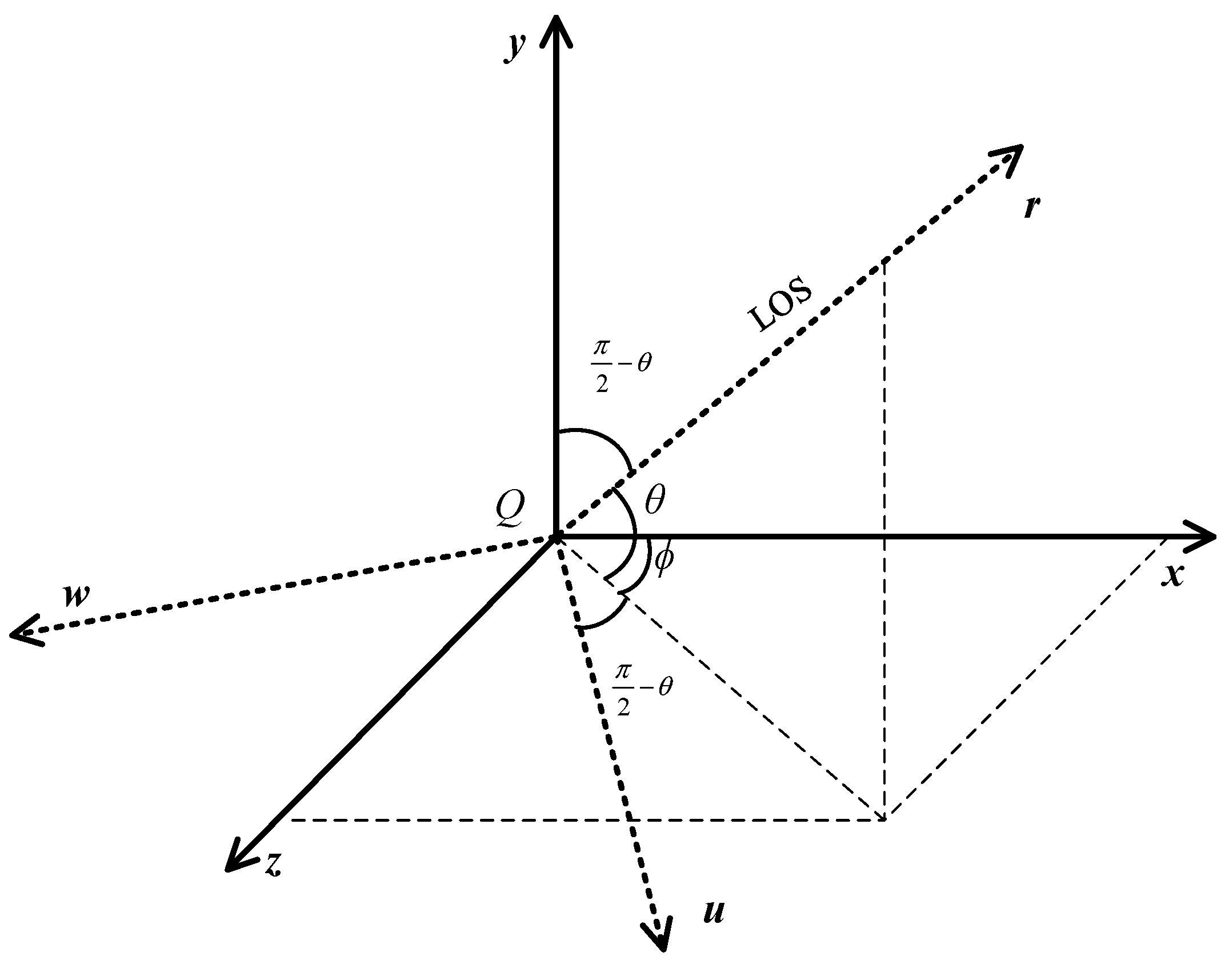
Another problem is that the y-coordinates of scatterers cannot be approximated by the LOS ranges any longer although the approximation is applicable in the normal model case, so the coordinate transformation is required for y-coordinate estimation. In Figure 3, the LOS coordinate system is denoted by (u, r, w), while the target coordinate system with the reference scatterer Q as the origin is denoted by (x, y, z). These two coordinates have the following rotational transformation relation:
where M is the rotation matrix as follows,
Therefore, yp can be obtained from (28)
where rP = RAP − RAQ. It should be noted that the Q does not need to be in the exact target center, because even if it is situated away from the target center by some distance (which depends on the accuracy of 3D locating of the target according to (14)), introducing some error on the y-coordinate estimation by coordinate transformation, the error is acceptable in consideration of the far-field condition.
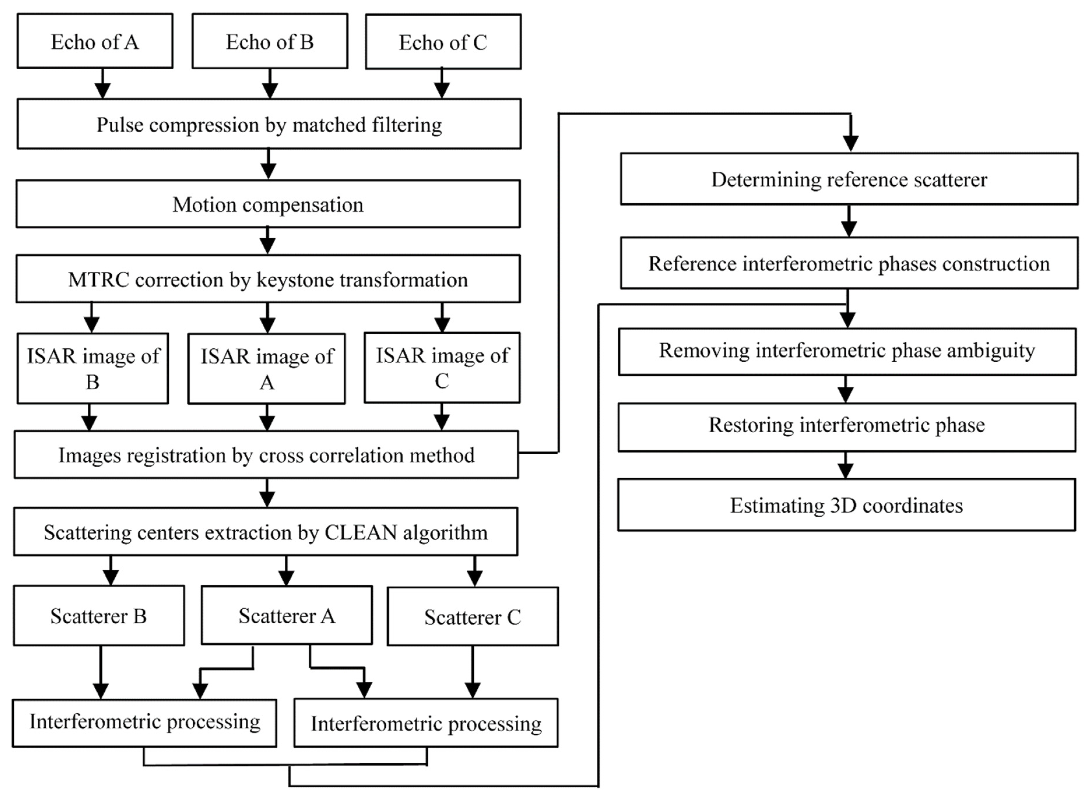
Figure 4 shows the complete flowchart of the proposed InISAR imaging method.
4. Simulation Results
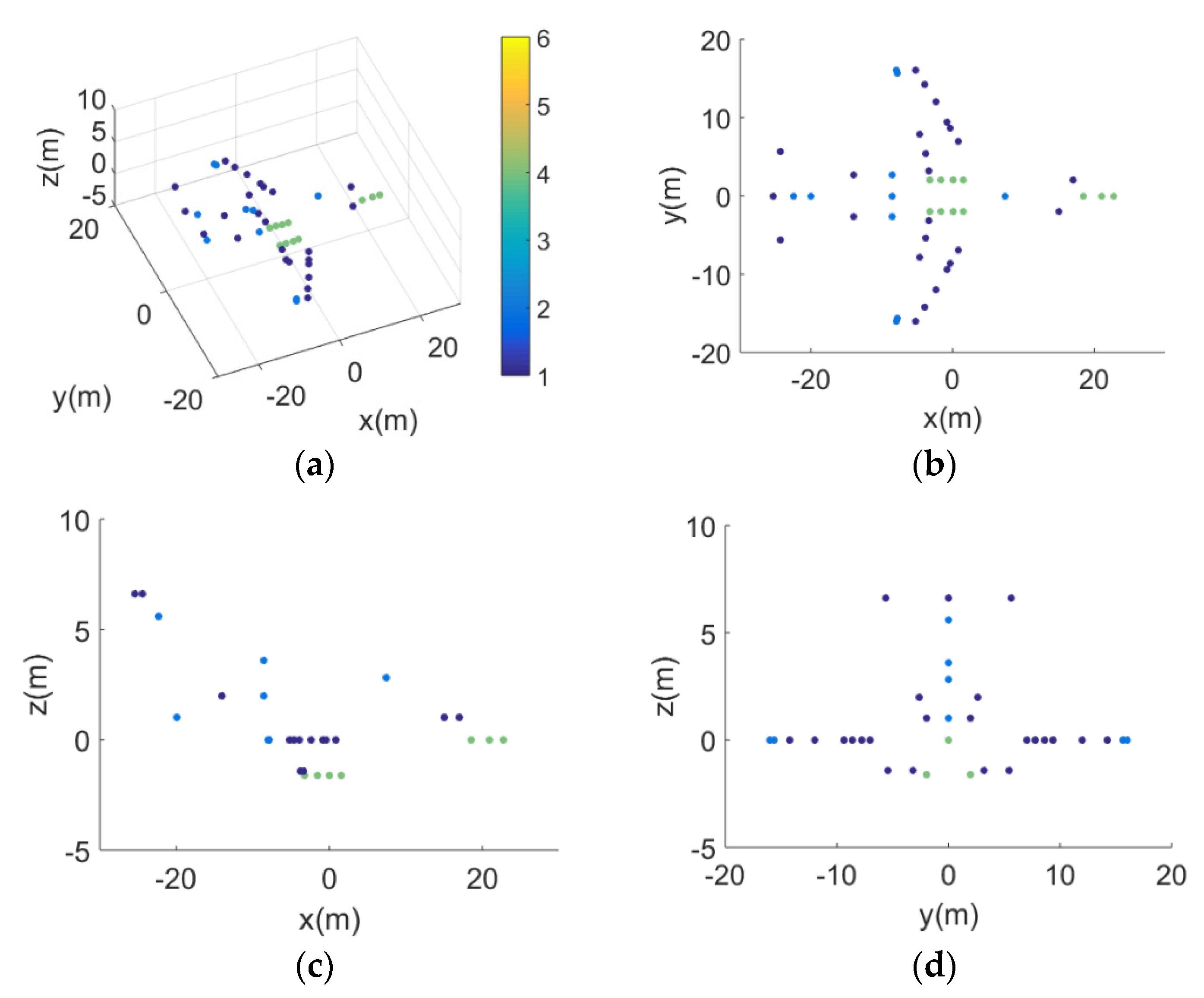
In order to verify the effectiveness of the proposed method, 3D InISAR imaging of a far-field target under squint geometry is simulated. The target is composed of point scatterers as shown in Figure 5 [3], where the color denotes the scattering intensity. Table 1 lists the major parameters for the simulated imaging system, obviously the target is far away from the antenna axis. The range resolution and cross-range resolution are calculated as 0.3 m and 0.5 m, respectively, according to the system parameters. And the real InPhas φAB and φAC calculated by substituting XP = YP = ZP = 10 km into Equations (8) and (9) are both about 120.91 radians, i.e., the InPhaA caused by the squint effect will appear inevitably. Moreover, the unambiguity ranges of xp and zp calculated by Equation (24) are ∈ (−260, 260) m, while the maximum dimension of the target is smaller than 50 m, so Equation (10) is satisfied, i.e., there is no InPhaA that can be caused by xp and zp. Therefore, we need to remove the influence of InPhaA caused by the squint effect.
4.1. Reference InPhas Construction
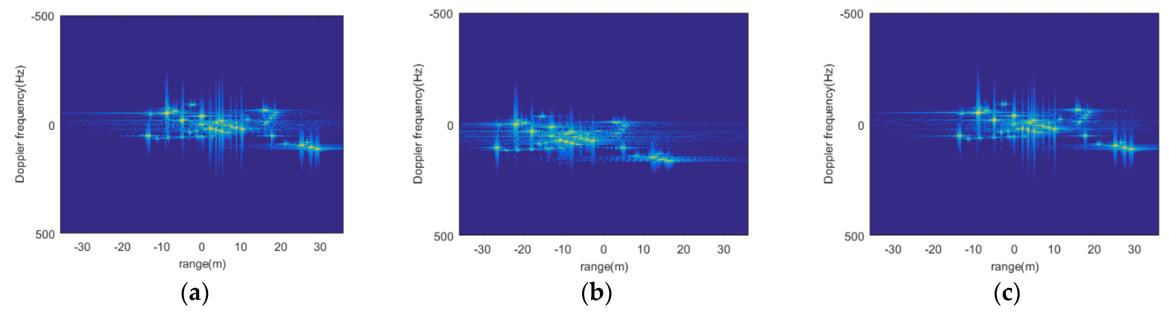
First, we need to obtain the target’s coarse 3D location. Based on the cross-correlation algorithm introduced in Section 3.1, the coarse location of the target is estimated by Equations (14)–(17) and the result is about (9.980, 9.939, 9.980) km, i.e., the relative location errors pertaining to the target center in X, Y, and Z coordinates are about 0.2%, 0.61%, and 0.2%, respectively. This coarse location is then taken as the reference scatterer Q to construct the reference InPhas by Equation (18). Although the location error looks large, it is actually within the constraints of Equation (19), i.e., the errors are within the acceptable range for the proposed imaging method. For better comparison, we display the ISAR image of antenna A obtained by the proposed method in Figure 6a, while presenting the ISAR images obtained by using the method of [25] in Figure 6b,c, respectively, by taking the Q and the target center as the reference scatterers. Compared with Figure 6a,b, it is not well focused visually, which is a result of the compensation error of the residual video phase induced by the dechirp processing when the distance between the reference scatterer and the target center exceeds a certain extent under the squint model. In order to quantify the focusing quality of images, we calculated the entropies and contrasts of Figure 6a–c and list them in Table 2. As can be seen, the image obtained by the proposed method has the smallest entropy while the largest contrast, i.e., it is best focused. However, the image obtained via the method in [25] by taking Q as the reference scatterer has the largest entropy while the smallest contrast, i.e., it is relatively not well focused, which will affect the subsequent extraction of scatterers, and definitely affect the estimation accuracy of the 3D coordinates of the scatterers.
4.2. InPhas Restoration
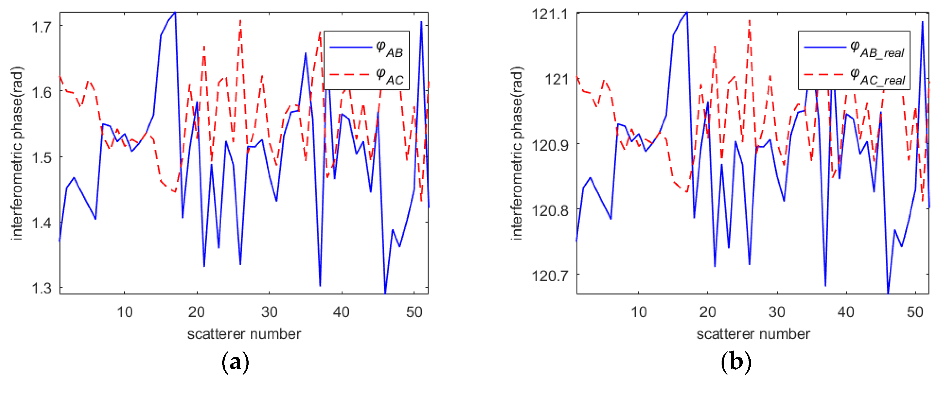
Before interferometric processing, image registrations are performed according to the results of Equation (17) and the scattering centers are extracted by the CLEAN algorithm [27]. Because the measured InPhas φAB_dir cannot exceed (−π, π), the real InPhas φAB_real should be the sum of φAB_dir and 2 kπ, where k is an integer to be decided. Figure 7a shows the measured InPhas directly obtained by the traditional InISAR imaging method, as it is shown, the φAB and φAB vary from 1.3 to 1.7 radians. They are ambiguous with 2 kπ radians absent according to the geometry. We used the constructed reference InPhas by Equations (20) and (21) to remove the InPhaA, and plot the real InPhas obtained by Equation (23) in Figure 7b. As can be clearly seen from Figure 7a,b, the InPhaA caused by the squint effect is eliminated, and the real InPhas of the all scatterers was successfully reconstructed.
4.3. 3D Coordinates Estimation
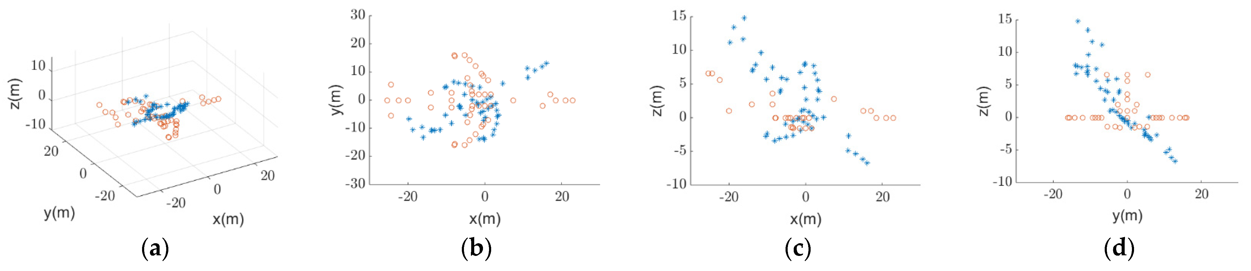
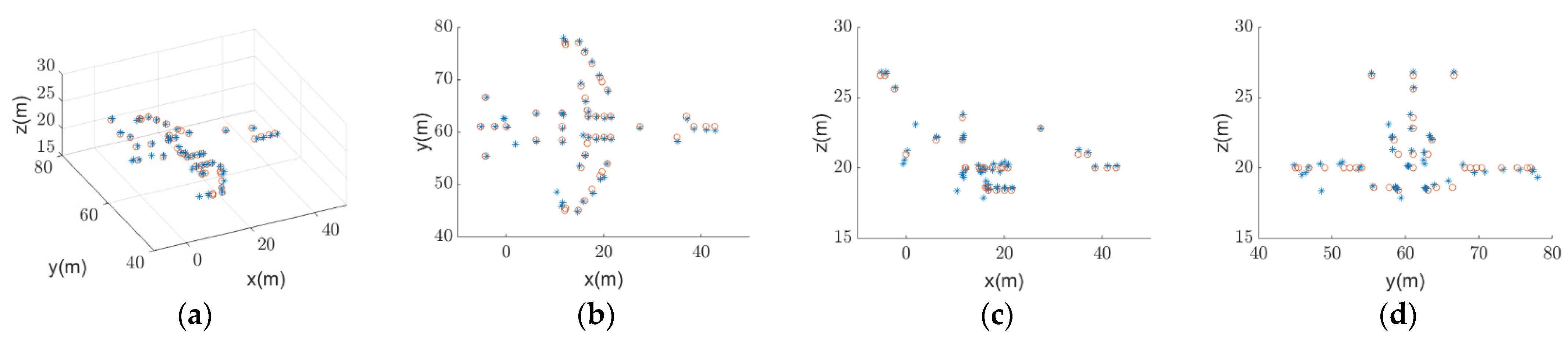
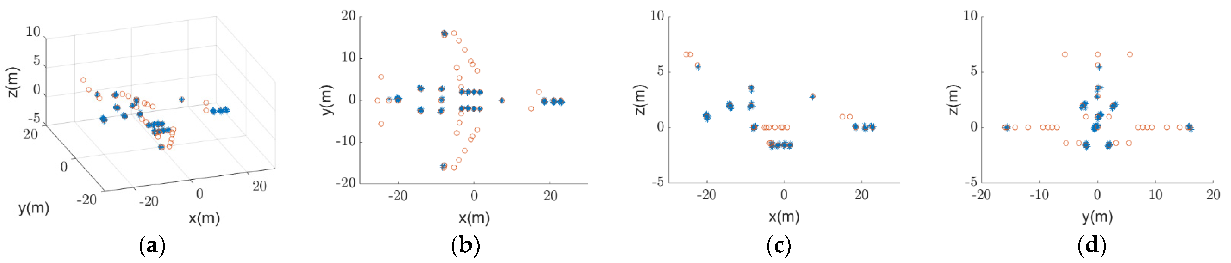
Finally, the restored real InPhas are used to estimate the coordinates along the baselines (i.e., x-coordinates and z-coordinates) for all scatterers by Equation (24), and then the y-coordinates are estimated by Equation (28). Figure 8 and Figure 9 present the 3D imaging results obtained by the traditional method and by the proposed method, respectively, where ‘*’ represents the reconstructed target and ‘o’ represents the model. As can be seen by comparing them, the reconstructed target by our method matches the target model very well, but that by the traditional method does not.
In the following, to better demonstrate the advantage of our method through quantitative comparison, two simulations are conducted by using the method in [25]: one is performed by taking the Q scatterer at position (9.980, 9.939, 9.980) km (obtained in Section 4.1) as the reference scatterer, and the another one is performed by taking the scatterer at position (9.995 9.995, 9.995) km as the reference scatterer, which is much closer to the target center with a relative error of 0.05% in X, Y, and Z coordinates. Figure 10 presents the first simulation results, which shows that the reconstructed 3D target is remarkably different from the target model; it cannot be used to effectively evaluate the reconstruction accuracy at all. The reason is due to the defocused ISAR images as shown in Figure 6b, which cannot be used to accurately extract the scatterers. Figure 11 presents the second simulation results. Although the reconstruction results are much better than that of Figure 10, they are still not as good as ours: the root mean square errors (RMSEs) of x, y, and z coordinates are all larger than ours as shown in Table 3. Nonetheless, the method in [25] is about 26 times slower than ours; both of them run in a computer with the Intel Core i5-8500 CPU of 3GB cache and 8GB memory. The high computational efficiency of our method is attributed to the direct estimation of 3D coordinates of scatterers without iteration.
4.4. Robustness of the Proposed Method
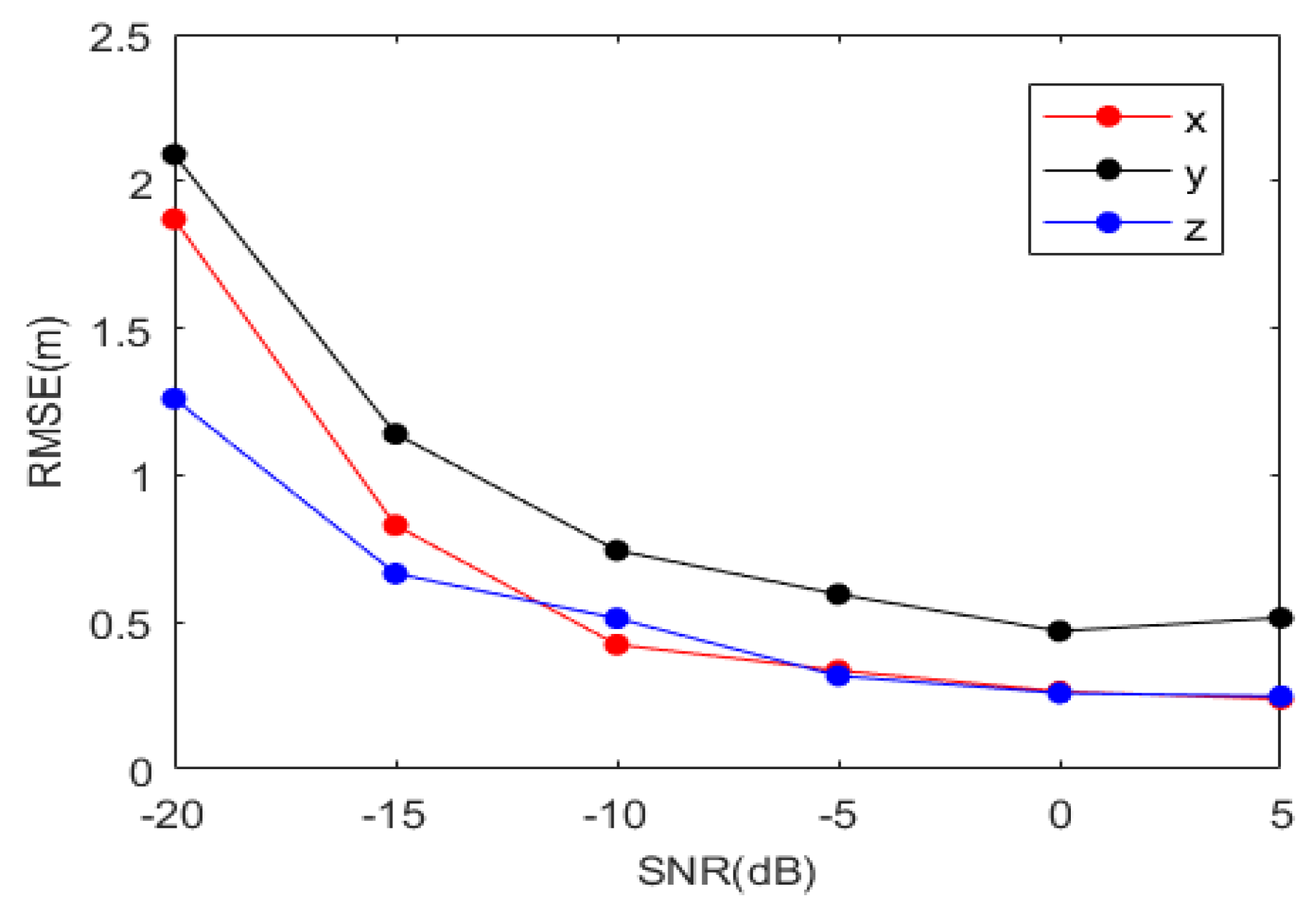
To evaluate the performance of the proposed method under noisy situations, simulations under different SNRs are conducted with the RMSEs of x, y, and z coordinates of all scatterers presented in Figure 12, from which one can see that the proposed method performs very well even if the SNR is as low as 0dB. As one can notice that the accuracy of the y coordinate reconstruction is always poorer than that of the x and z coordinates in all SNR cases, which can be attributed to the cascading of errors since the estimation of y coordinate depends on the estimation of x and z coordinates as shown by Equation (28)
5. Experiment Results
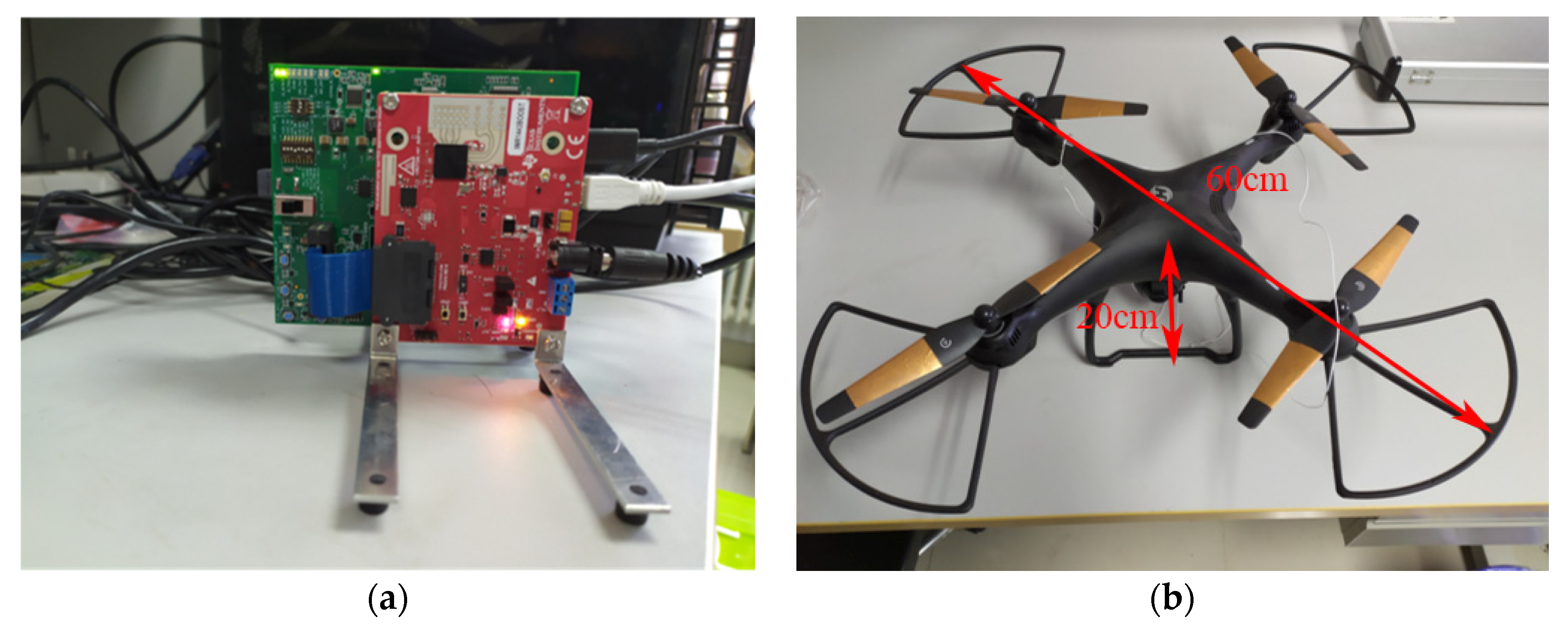
To validate the proposed method rigorously, we carried out a practical experiment using a radar demo system with an AWR1243 produced by Texas Instruments as shown in Figure 13a, to image a rotating unmanned aerial vehicle (UAV) shown in Figure 13b. The radar includes three transmitting antennas (TX1, TX2, TX3) and four receiving antennas (RX1, RX2, RX3, RX4). Figure 14a presents the simplified observation geometry for describing the experiment clearly. The antennas appear to not be positioned in the L-shape or cross-shape that the traditional 3D InISAR imaging methods usually rely on, however they can be configured to an L-type as follows. First, a 3D coordinate system is established by taking the transmitting antenna TX1 as the origin, so the coordinates of TX2, RX4, RX1, and RX2 can be obtained as (−λ, 0, λ/2), (d, 0, 0), (d + 3λ/2, 0, 0) and (d + λ, 0, 0), respectively. This configuration guarantees that a moderate bistatic acquisition geometry can be obtained, which can then be approximated by an equivalent monostatic acquisition geometry with virtual self-transmitting and self-receiving antennas positioned in the middle of the original transmitting antennas and receiving antennas [28]. Therefore, the echo from TX1 transmitting and RX4 receiving (1T4R) can be equivalent to the echo from a virtual self-transmitting and self-receiving antenna at A(d/2, 0, 0). Similarly, the echoes from 1T1R and 2T2R can be equivalent to the echoes from self-transmitting and self-receiving antennas at B(d/2 + 3λ/4, 0, 0) and C(d/2, 0, λ/4), respectively. Obviously, the three virtual antennas A, B, and C form an L-type InISAR system as shown in Figure 14b, which is then used to verify the proposed method. Table 4 lists some typical parameters of the experiment system. The length and height of the UAV are about 0.6 m and 0.2 m, respectively, and the target center is approximately positioned at (0.5, 1.1, 0.1) m as shown in Figure 13b. Suppose P is an arbitrarily selected scattering center from the UAV, then XP ∈ (0.2, 0.8) and ZP ∈ (0, 0.2). Then, the range of InPhas can be roughly estimated according to Equations (4) and (5), i.e., φAB_real ∈ (π/2, 2π), and φAC_real ∈ (0, π/2), and it is apparent that the InPhas of the all scattering centers from the Z-direction interferometry are within (−π, π), while the InPhas of some scattering centers from the X-direction interferometry exceed (−π, π), which is caused by the squint effect as mentioned in Section 2, that is to say, the InPhaA occurs, which must be removed before imaging processing. The above analysis is validated by the results shown in Figure 15.
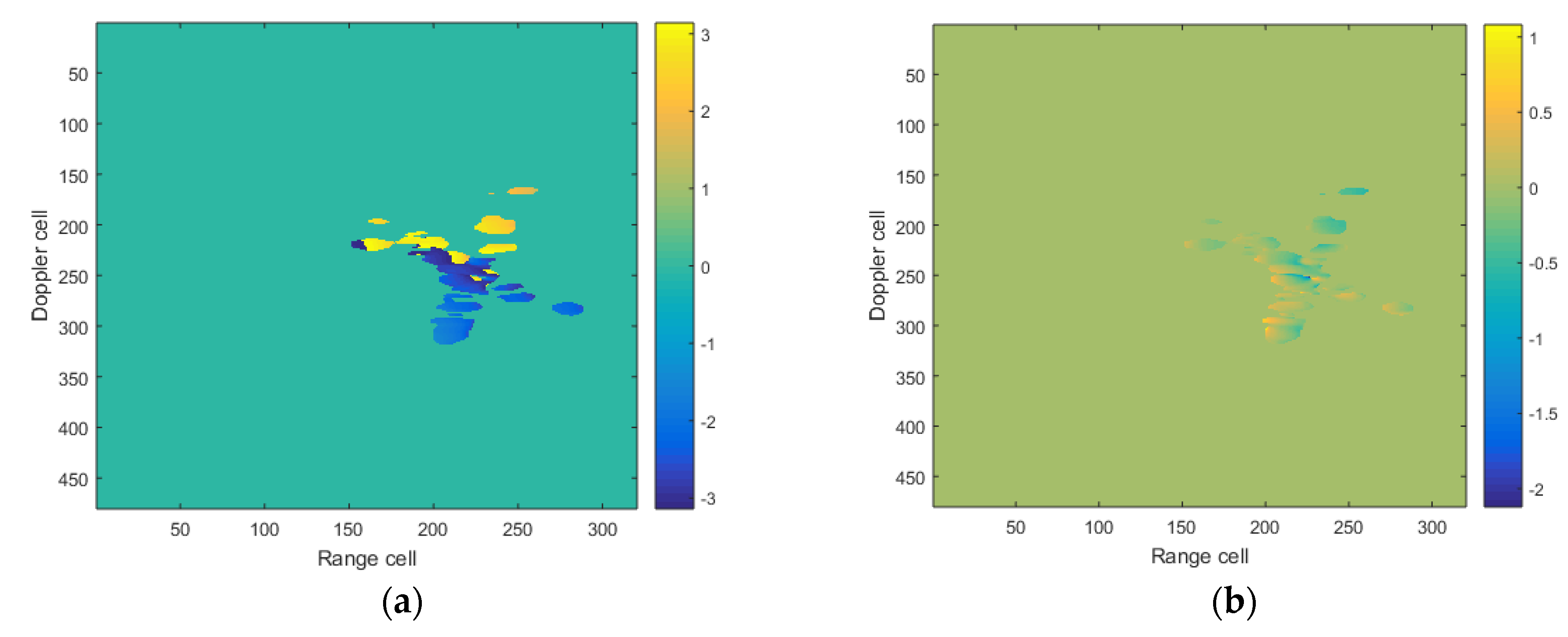
After imaging processing and image registration, the InPha images of measured InPhas from both the X-direction and the Z-direction interferometries are obtained and shown in Figure 15a,b, respectively. As shown in Figure 15a, there are obvious discontinuities in the InPha distribution, which is due to the InPhaA caused by the squint effect. Different from the InPha curves in Figure 7a, the InPhaA in the experiment appears as an abrupt change of colors between scatterers because the InPha is denoted by color.
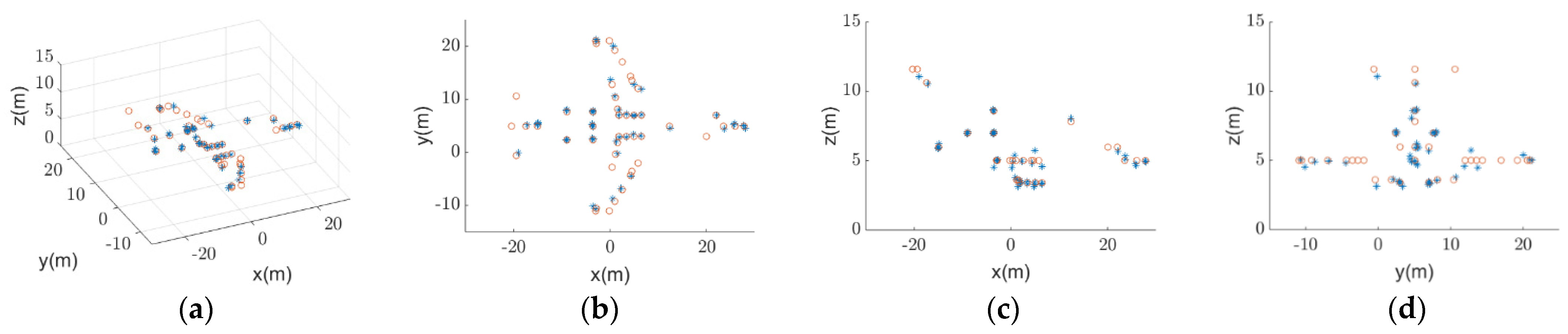
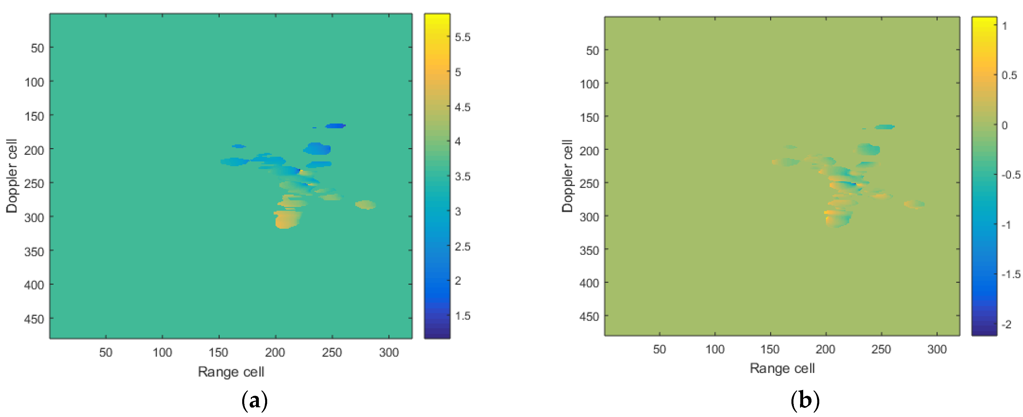
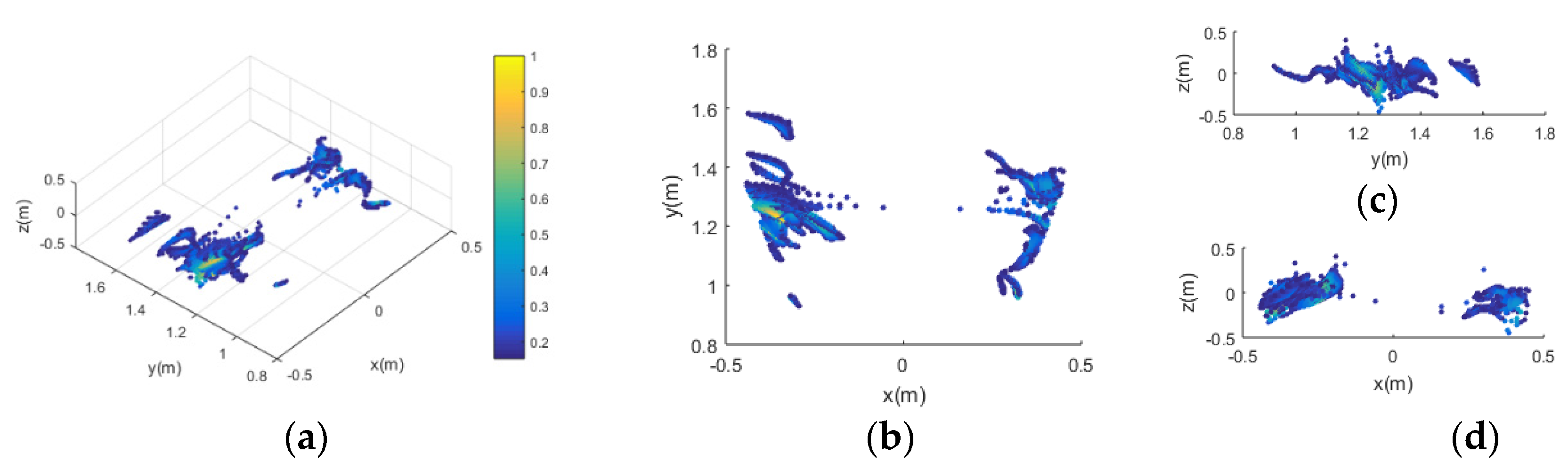
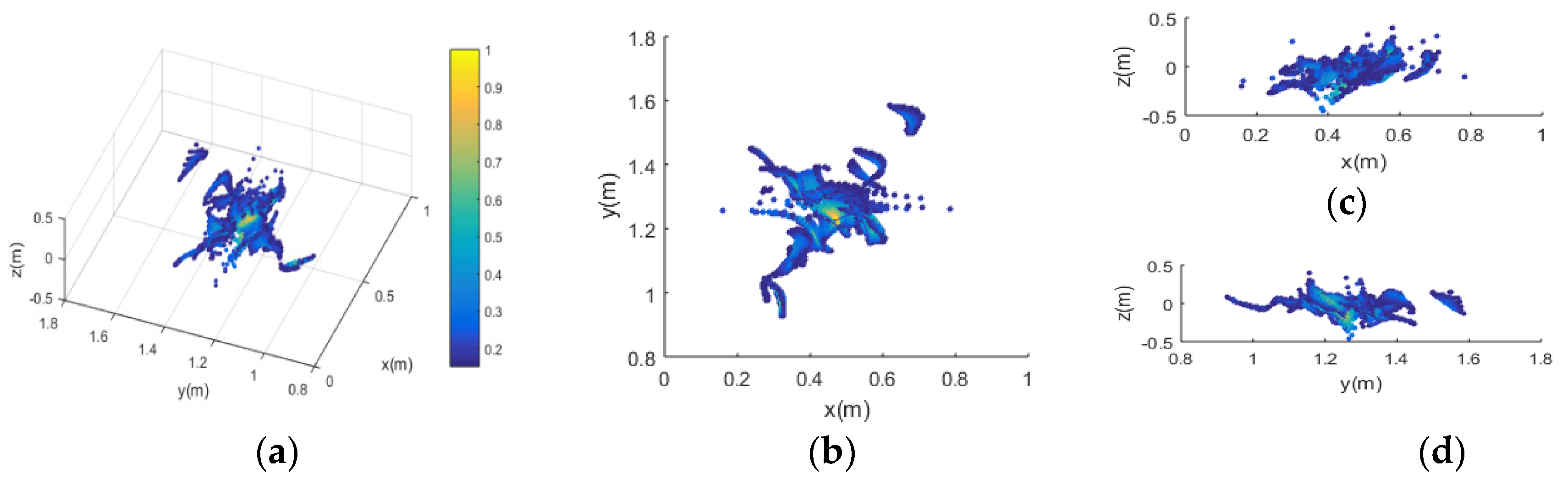
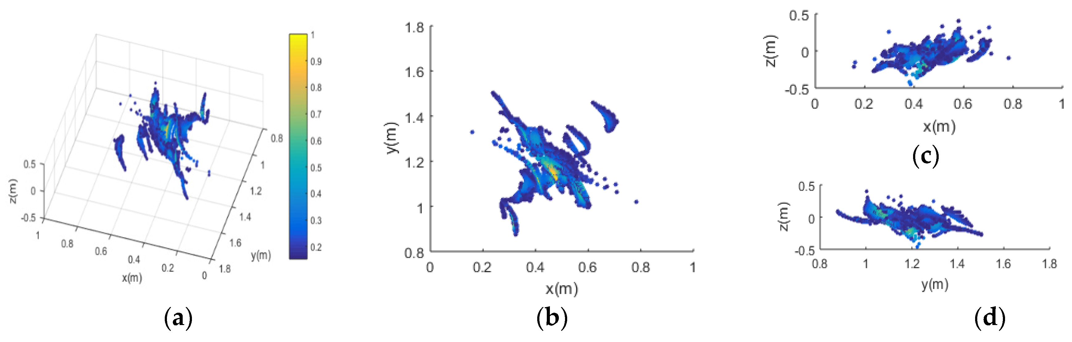
In order to eliminate the InPhaA and restore the real InPha, we need to know the target’s coarse 3D location. We estimated the wave path difference along the X direction by performing the cross-correlation processing on the ISAR images of 1T4R and 1T1R, while we estimated the wave path difference along the Z direction by performing the cross-correlation processing on the ISAR images of 2T2R and 1T1R. We interpolated the ISAR images by 32 times to guarantee the estimation accuracy. Then, the coarse location of the target is estimated according to Equation (14) and the result is (0.5692, 1.212, 0) km, which is then taken as the coordinates of the reference scatterer Q to construct the reference InPhas. Then, the real InPhas are calculated by Equations (16)–(19) and the obtained unambiguous InPha images are shown in Figure 16. As can be seen by comparing Figure 16a with Figure 15a, the discontinuities of InPhas disappear, meaning that the InPhaA is eliminated. By comparing Figure 16b with Figure 15b, it is apparent that the InPhas are the same before and after InPhaA removal. This is because there is no InPhaA in the Z-direction. Figure 17 and Figure 18 show the 3D imaging results before and after the InPhaA removal, respectively. Although the images of Figure 18 demonstrate the approximate outlines of the target, they are still slightly distorted particularly in the x-y plane. Figure 19 presents the final imaging results after the distortion was corrected through coordinate transformation, which shows that the x-y plane result is closer to the real shape.
6. Conclusions
In this paper, we propose a squint model InISAR imaging method based on reference InPhas construction and coordinate transformation. In this approach, a reference scatterer within a coarsely reconstructed 3D target by the cross-correlation method is first selected, which is used to construct the reference InPhas for removing the phase ambiguities. Then, the InPhaA caused by the squint effect is removed and the real InPhas are restored. Finally, the image distortion is successfully corrected by coordinate transformation. Both simulation and experiment results demonstrated the effectiveness of the proposed method very well. It is shown that the reconstruction accuracy of the 3D position of the target improves as the SNR increases and the simulations show a less than 0.3 m error for X and Z coordinates and a less than 0.6 m error for Y coordinate can be achieved under our simulation geometry with a SNR of 5 dB. The InPha-related accuracy issue of 3D target reconstruction under different observation geometries deserves to be investigated in the future.
Author Contributions
Conceptualization, Y.L. and Y.Z.; methodology, Y.L. and X.D.; software, Y.L and X.D.; validation, Y.L., X.D. and Y.Z.; formal analysis, Y.L.; investigation, Y.L.; resources, Y.Z.; data curation, X.D.; writing—original draft preparation, Y.L.; writing—review and editing, Y.Z.; visualization, Y.L.; supervision, Y.Z.; project administration, Y.Z.; funding acquisition, Y.Z. All authors have read and agreed to the published version of the manuscript.
Funding
This research was funded by the National Natural Science Foundation of China under Grant 61971402.
Conflicts of Interest
The authors declare no conflict of interest.
References
- Chen, C.C.; Andrews, H.C. Target-Motion-Induced Radar Imaging. IEEE Trans. Aerosp. Electron. Syst. 1980, 16, 2–14. [Google Scholar] [CrossRef]
- Walker, J.L. Range-Doppler Imaging of Rotating Objects. IEEE Trans. Aerosp. Electron. Syst. 1980, 16, 23–52. [Google Scholar] [CrossRef]
- Chen, V.C.; Martorella, M. Inverse Synthetic Aperture Radar Imaging: Principles, Algorithms and Applications; John Wiley & Sons. Inc: Hoboken, NJ, USA, 2014; pp. 121–168. [Google Scholar]
- Xu, X.; Narayanan, R.M. Enhanced resolution in SAR/ISAR imaging using iterative sidelobe apodization. IEEE Trans. Image Process. 2005, 14, 537–547. [Google Scholar] [PubMed]
- Zhang, J.; Liao, G.; Zhu, S.; Xu, J.; Huo, L.; Yang, J. An Efficient ISAR Imaging Method for Non-Uniformly Rotating Targets Based on Multiple Geometry-Aided Parameters Estimation. IEEE Sens. J. 2018, 19, 2191–2204. [Google Scholar] [CrossRef]
- Gao, Y.; Xing, M.; Zhang, Z.; Liang, G. ISAR Imaging and Cross-Range Scaling for Maneuvering Targets by Using the NCS-NLS Algorithm. IEEE Sens. J. 2019, 19, 4889–4897. [Google Scholar] [CrossRef]
- Xu, G.; Xing, M.; Xia, X.-G.; Zhang, L.; Chen, Q.; Bao, Z. 3D Geometry and Motion Estimations of Maneuvering Targets for Interferometric ISAR With Sparse Aperture. IEEE Trans. Image Process. 2016, 25, 2005–2020. [Google Scholar] [CrossRef]
- Zhao, L.; Gao, M.; Martorella, M.; Stagliano, D. Bistatic three-dimensional interferometric ISAR image reconstruction. IEEE Trans. Aerosp. Electron. Syst. 2015, 51, 951–961. [Google Scholar] [CrossRef]
- Yong, W.; Li, X. Three-Dimensional Interferometric ISAR Imaging for the Ship Target Under the Bi-Static Configuration. IEEE J. Sel. Top. Appl. Earth Obs. Remote Sens. 2016, 9, 1–16. [Google Scholar]
- Felguera-Martín, D.; González-Partida, J.-T.; Almorox-González, P.; Burgos-García, M. Interferometric inverse synthetic aperture radar experiment using an interferometric linear frequency modulated continuous wave millimetre-wave radar. Iet Radar Sonar Navig. 2011, 5, 39–47. [Google Scholar] [CrossRef] [Green Version]
- Liu, B.; Pan, Z.-H.; Li, D.-J.; Qiao, M. Moving target detection and location based on millimeter-wave InISAR imaging. J. Infrared Millim. Waves 2012, 31, 258–264. [Google Scholar] [CrossRef]
- Wang, Y.; Huang, X.; Cao, R. Novel Method of ISAR Cross-Range Scaling for Slowly Rotating Targets Based on the Iterative Adaptive Approach and Discrete Polynomial-Phase Transform. IEEE Sens. J. 2019, 19, 4898–4906. [Google Scholar] [CrossRef]
- Given, J.A.; Schmidt, W.R. Generalized ISAR—Part II: Interferometric techniques for three-dimensional location of scatterers. IEEE Trans. Image Process. 2005, 14, 1792–1797. [Google Scholar] [CrossRef] [PubMed]
- Wang, G.; Xia, X.G.; Chen, V.C. Three-dimensional ISAR imaging of maneuvering targets using three receivers. IEEE Trans. Image Process. 2002, 10, 436–447. [Google Scholar] [CrossRef]
- Xu, X.; Narayanan, R.M. Three-dimensional interferometric ISAR imaging for target scattering diagnosis and modeling. IEEE Trans. Image Process. 2001, 10, 1094–1102. [Google Scholar] [PubMed]
- Zhang, Q.; Yeo, T.S. Three-dimensional SAR imaging of a ground moving target using the InISAR technique. IEEE Trans. Geosci. Remote. Sens. 2004, 42, 1818–1828. [Google Scholar] [CrossRef]
- Zhang, Q.; Yeo, T.S.; Gan, D.; Zhang, S. Estimation of Three-Dimensional Motion Parameters in Interferometric ISAR Imaging. IEEE Trans. Geosci. Remote Sens. 2004, 42, 292–300. [Google Scholar] [CrossRef]
- Battisti, N.; Martorella, M. Intereferometric phase and target motion estimation for accurate 3D reflectivity reconstruction in ISAR systems. In Proceedings of the 2010 IEEE Radar Conference, Arlington, VA, USA, 10–14 May 2010. [Google Scholar]
- Martorella, M.; Stagliano, D.; Salvetti, F.; Battisti, N. 3D interferometric ISAR imaging of noncooperative targets. IEEE Trans. Aerosp. Electron. Syst. 2014, 50, 3102–3114. [Google Scholar] [CrossRef]
- Bao, Z.; Xing, M.; Wang, T. Radar Imaging Technology; Publishing House of Electronics Industry: Beijing, China, 2004; pp. 277–326. [Google Scholar]
- Tian, B.; Lu, Z.; Liu, Y.; Li, X. Review on Interferometric ISAR 3D Imaging: Concept, Technology and Experiment. Signal Process. 2018, 153, 164–187. [Google Scholar] [CrossRef]
- Ma, C.Z.; Yeo, T.S.; Tan, H.S.; Lu, G. Interferometric ISAR imaging on squint model. Prog. Electromagn. Res. Lett. 2008, 2, 125–133. [Google Scholar] [CrossRef] [Green Version]
- Li, L.; Liu, H.; Jiu, B. An interferometric inverse synthetic aperture radar imaging algorithms for squint model. Xi’an Jiaotong Univ. 2008, 42, 1290–1294. [Google Scholar]
- Liu, C.L.; Feng, H.E.; Gao, X.Z.; Xiang, L.I.; Shen, R.J. Squint-mode InISAR imaging based on nonlinear least square and coordinates transform. Sci. China Technol. Sci. 2011, 054, 3332–3340. [Google Scholar] [CrossRef]
- Tian, B.; Zou, J.; Xu, S.; Chen, Z. Squint model interferometric ISAR imaging based on respective reference range selection and squint iteration improvement. IET Radar Sonar Navig. Iet 2015, 9, 1366–1375. [Google Scholar] [CrossRef]
- Yuan, Z.; Wang, J.; Zhao, L.; Xiong, D.; Gao, M. Phase Unwrapping for Bistatic InISAR Imaging of Space Targets. IEEE Trans. Aerosp. Electron. Syst. 2019, 55, 1794–1805. [Google Scholar] [CrossRef]
- Bose, R.; Fr Ee Dman, A.; Steinberg, B.D. Sequence CLEAN: A modified deconvolution technique for microwave images of contiguous targets. IEEE Trans. Aerosp. Electron. Syst. 2002, 38, 89–97. [Google Scholar] [CrossRef]
- Johnson, J.; Gupta, I.; Burkholder, R. Comparison of Monostatic and Bistatic Radar Images. IEEE Antenna Propag. Mag. 2003, 45, 41–50. [Google Scholar]
Figure 1.
InISAR imaging under squint model.

Figure 2.
The influence of the squint effect on InPhas: (a) the real InPha; (b) the measured InPhas.
Figure 2.
The influence of the squint effect on InPhas: (a) the real InPha; (b) the measured InPhas.

Figure 3.
Rotation of coordinate systems.

Figure 4.
Flowchart of the proposed InISAR imaging method.

Figure 5.
Target model in (a) 3D; (b) projection on x-y plane; (c) projection on x-z plane; (d) projection on y-z plane.
Figure 5.
Target model in (a) 3D; (b) projection on x-y plane; (c) projection on x-z plane; (d) projection on y-z plane.

Figure 6.
ISAR images of antenna A obtained by (a) the proposed method; (b) the method in [25] by taking Q as the reference scatterer; (c) the method in [25] by taking the target center as the reference scatterer.

Figure 7.
Interferometric phases: (a) before InPha restoration; (b) after InPha restoration.

Figure 8.
3D imaging results by the traditional method without removing the squint effect, in (a) 3D; (b) projection on x-y plane; (c) projection on x-z plane; (d) projection on y-z plane.
Figure 8.
3D imaging results by the traditional method without removing the squint effect, in (a) 3D; (b) projection on x-y plane; (c) projection on x-z plane; (d) projection on y-z plane.

Figure 9.
3D imaging results obtained by the proposed method with the Q scatterer at position (9.980, 9.939, 9.980) km taken as the reference scatterer in (a) 3D; (b) projection on x-y plane; (c) projection on x-z plane; (d) projection on y-z plane.
Figure 9.
3D imaging results obtained by the proposed method with the Q scatterer at position (9.980, 9.939, 9.980) km taken as the reference scatterer in (a) 3D; (b) projection on x-y plane; (c) projection on x-z plane; (d) projection on y-z plane.

Figure 10.
3D imaging results obtained by the method in [25] with the Q scatterer at position (9.980, 9.939, 9.980) km taken as the reference scatterer in (a) 3D; (b) projection on x-y plane; (c) projection on x-z plane; (d) projection on y-z plane.
Figure 10.
3D imaging results obtained by the method in [25] with the Q scatterer at position (9.980, 9.939, 9.980) km taken as the reference scatterer in (a) 3D; (b) projection on x-y plane; (c) projection on x-z plane; (d) projection on y-z plane.

Figure 11.
3D imaging results obtained by the method in [25] with the scatterer at position (9.995, 9.995, 9.995) km taken as the reference scatterer in (a) 3D; (b) projection on x-y plane; (c) projection on x-z plane; (d) projection on y-z plane.
Figure 11.
3D imaging results obtained by the method in [25] with the scatterer at position (9.995, 9.995, 9.995) km taken as the reference scatterer in (a) 3D; (b) projection on x-y plane; (c) projection on x-z plane; (d) projection on y-z plane.

Figure 12.
RMSE under different SNR.

Figure 13.
Radar system and target: (a) the InISAR system; (b) the rotating target.

Figure 14.
Experiment observation geometry: (a) real observation geometry; (b) equivalent observation geometry.
Figure 14.
Experiment observation geometry: (a) real observation geometry; (b) equivalent observation geometry.

Figure 15.
InPha images of measured InPhas: (a) from X-direction interferometry, the InPha is discontinuous as indicated by the abrupt change of colors between yellow and dark blue; (b) from Z-direction interferometry, the InPha is continuous as indicated by the gradual change of colors between yellow and light blue.

Figure 16.
InPha images of real InPhas: (a) from X-direction interferometry, the InPha is continuous as indicated by the gradual change of colors between yellow and light blue; (b) from Z-direction interferometry, the InPha is continuous as indicated by the gradual change of colors between yellow and light blue.

Figure 17.
Three-dimensional imaging results without InPhaA removed: (a) 3D reconstruction; (b) projection on x-y plane; (c) projection on x-z plane; (d) projection on y-z plane.
Figure 17.
Three-dimensional imaging results without InPhaA removed: (a) 3D reconstruction; (b) projection on x-y plane; (c) projection on x-z plane; (d) projection on y-z plane.

Figure 18.
Three-dimensional imaging results with InPhaA removed (a) 3D reconstruction; (b) projection on x-y plane; (c) projection on x-z plane; (d) projection on y-z plane.
Figure 18.
Three-dimensional imaging results with InPhaA removed (a) 3D reconstruction; (b) projection on x-y plane; (c) projection on x-z plane; (d) projection on y-z plane.

Figure 19.
Three-dimensional imaging results with InPhaA removed and image distortion corrected: (a) 3D reconstruction; (b) projection on x-y plane; (c) projection on x-z plane; (d) projection on y-z plane.
Figure 19.
Three-dimensional imaging results with InPhaA removed and image distortion corrected: (a) 3D reconstruction; (b) projection on x-y plane; (c) projection on x-z plane; (d) projection on y-z plane.


Table 1.
Simulation parameters of the InISAR system.
| Parameters | Value |
|---|---|
| Carrier frequency | 10 GHz |
| Bandwidth | 500 MHz |
| PRF | 500 Hz |
| Location of antenna A | (0,0,0) |
| Location of antenna B | (1,0,0) m |
| Location of antenna C | (0,0,1) m |
| Target velocity | 50 m/s |
| Roll/pitch/yaw | 0/0/0.03 rad/s |
| SNR | 10 dB |
| Target location | (10,10,10) km |
| θ | 45 deg |
| φ | 45 deg |
Table 2.
Comparison of image entropy and contrast.
| Image Entropy | Image Contrast | |
|---|---|---|
| Figure 6a | 3.95 | 7.48 |
| Figure 6b | 4.08 | 6.01 |
| Figure 6c | 4.05 | 6.39 |
Table 3.
Comparison of RMSEs and runtimes of our method and the method in [25].
Table 3.
Comparison of RMSEs and runtimes of our method and the method in [25].
| Method | RMSE of x | RMSE of y | RMSE of z | Runtime |
|---|---|---|---|---|
| Our method | 0.2063 | 0.3389 | 0.1914 | 0.01 s |
| Ref. [25] | 0.2125 | 0.3734 | 0.2195 | 0.26 s |
Table 4.
Parameters of the experiment system.
| Parameters | Value |
|---|---|
| Carrier frequency | 77 GHz |
| Chirp rate | 39.976 MHz |
| Pulse width | 100 μs |
| PRF | 200 Hz |
| Rotational velocity | 0.2618 rad/s |
| Imaging time | 0.6 s |
Publisher’s Note: MDPI stays neutral with regard to jurisdictional claims in published maps and institutional affiliations. |
© 2021 by the authors. Licensee MDPI, Basel, Switzerland. This article is an open access article distributed under the terms and conditions of the Creative Commons Attribution (CC BY) license (https://creativecommons.org/licenses/by/4.0/).
Share and Cite
MDPI and ACS Style
Li, Y.; Zhang, Y.; Dong, X. Squint Model InISAR Imaging Method Based on Reference Interferometric Phase Construction and Coordinate Transformation. Remote Sens. 2021, 13, 2224. https://0-doi-org.brum.beds.ac.uk/10.3390/rs13112224
AMA Style
Li Y, Zhang Y, Dong X. Squint Model InISAR Imaging Method Based on Reference Interferometric Phase Construction and Coordinate Transformation. Remote Sensing. 2021; 13(11):2224. https://0-doi-org.brum.beds.ac.uk/10.3390/rs13112224
Chicago/Turabian StyleLi, Yu, Yunhua Zhang, and Xiao Dong. 2021. "Squint Model InISAR Imaging Method Based on Reference Interferometric Phase Construction and Coordinate Transformation" Remote Sensing 13, no. 11: 2224. https://0-doi-org.brum.beds.ac.uk/10.3390/rs13112224
Note that from the first issue of 2016, this journal uses article numbers instead of page numbers. See further details here.