Validation of Sentinel-3 SLSTR Land Surface Temperature Retrieved by the Operational Product and Comparison with Explicitly Emissivity-Dependent Algorithms

Abstract

Land surface temperature (LST) is an essential climate variable (ECV) for monitoring the Earth climate system. To ensure accurate retrieval from satellite data, it is important to validate satellite derived LSTs and ensure that they are within the required accuracy and precision thresholds. An emissivity-dependent split-window algorithm with viewing angle dependence and two dual-angle algorithms are proposed for the Sentinel-3 SLSTR sensor. Furthermore, these algorithms are validated together with the Sentinel-3 SLSTR operational LST product as well as several emissivity-dependent split-window algorithms with in-situ data from a rice paddy site. The LST retrieval algorithms were validated over three different land covers: flooded soil, bare soil, and full vegetation cover. Ground measurements were performed with a wide band thermal infrared radiometer at a permanent station. The coefficients of the proposed split-window algorithm were estimated using the Cloudless Land Atmosphere Radiosounding (CLAR) database: for the three surface types an overall systematic uncertainty (median) of −0.4 K and a precision (robust standard deviation) 1.1 K were obtained. For the Sentinel-3A SLSTR operational LST product, a systematic uncertainty of 1.3 K and a precision of 1.3 K were obtained. A first evaluation of the Sentinel-3B SLSTR operational LST product was also performed: systematic uncertainty was 1.5 K and precision 1.2 K. The results obtained over the three land covers found at the rice paddy site show that the emissivity-dependent split-window algorithms, i.e., the ones proposed here as well as previously proposed algorithms without angular dependence, provide more accurate and precise LSTs than the current version of the operational SLSTR product.

1. Introduction

Land surface temperature (LST)—like near-surface air temperature—is a key variable in a wide variety of studies, since it is linked to land–atmosphere energy transfer and flux balances [1,2]. Thus, it is required for monitoring evapotranspiration and climate change [3,4], as well as for providing estimates of fire size and temperature [5,6], volcanoes and lava flow [7,8], and vegetation health [9,10,11]. According to the Global Climate Observing System [12], the World Meteorological Organization (WMO) considers LST as one of the essential climate variables (ECVs). The Climate Change Initiative (CCI) was launched by the European Space Agency (ESA) for improving the prediction of climate change trends by means of satellite data [13]. The CCI considers LST an important variable for monitoring the Earth climate system; therefore, they included it in the list of ECVs required for understanding and predicting the evolution of climate (http://cci.esa.int/ (accessed on 1 March 2021)). Consequently, the validation of satellite derived LSTs against independent references is crucial for assessing their accuracy and precision. For LST retrieval from satellite data, the GCOS set the recommended thresholds on accuracy (bias, defined as the systematic uncertainty by the Joint Committee for Guides in Metrology [14], JCGM) and precision (standard deviation, SD, defined as the random uncertainty by the JCGM [14]) to 1 K [12].

The Sea and Land Surface Temperature Radiometer (SLSTR) on board the Sentinel-3A and 3B spacecrafts is a follow-on instrument of the Advanced Along-Track Scanning Radiometer (AATSR). The two sensors have similar characteristics, including their thermal channels at 11 and 12 µm, with double view capability, and allow us to apply split-window algorithms (SWAs) and dual-angle algorithms (DAAs). In this paper, the SWA proposed by Niclòs et al. in [15] and the DAA proposed by Coll et al. in [16] were adapted to SLSTR’s thermal bands. The SWA proposed by Niclòs et al. in [15] was developed for the Spinning Enhanced Visible and InfraRed Imager (SEVIRI) onboard Meteosat Second Generation (MSG) and depends explicitly on emissivity and view zenith angle. SLSTR has view zenith angles up to 60° [17] and, thus, angular anisotropy may have an important impact on LST retrieval, which was noticed when analyzing the angular dependence of the SWA’s regression coefficients. For the SEVIRI sensor, over the rice paddy site, the SWA proposed by Niclòs et al. in [15] provided an accuracy (bias) and precision (SD) of 0.5 and 0.8 K, respectively. The capability of the AATSR sensor to apply the DAA was previously analyzed in [16] over full vegetation cover. These authors proposed and validated a SWA and a DAA, obtaining a higher standard deviation for the DAA, with accuracy (precision) of 0.0 K (1.0 K). They concluded that the DAA performed worse than the SWA, mainly due to differences between the nadir and oblique footprints [16].

The operational LST level 2 (L2) product for the SLSTR sensor is generated with a SWA whose coefficients depend on surface biome, water vapor content (WVC) in the atmosphere, and vegetation fraction cover [18,19]. Previous studies validated the Sentinel-3A SLSTR operational LST product over a variety of surfaces, but not over a rice paddy. In the ESA validation report, 11 sites were used to validate the SLSTR LST product over different land covers [20]: seven were stations of the SURFace RADiance (SURFRAD) network, which uses pyrgeometers (3–50 µm), three were stations of the Karlsruhe Institute Technology (KIT) equipped with narrow band radiometers (9.6–11.5 µm), and one was the U.S. Department of Energy’s Atmospheric Radiation Measurement (ARM) station equipped with narrow band radiometers.

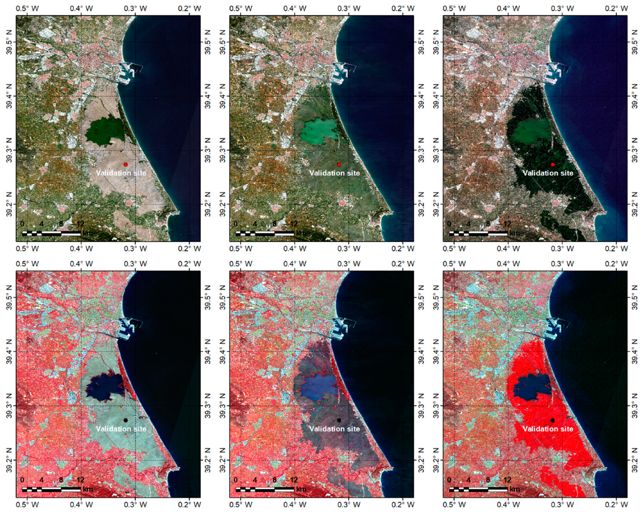
In this paper, phenological changes of a rice paddy during the growing period were used to validate the SLSTR LST product over three different surfaces: bare soil (wet and dry), water (flooded surfaces), and full vegetation cover. A permanent station with a wide band Thermal Infrared (TIR) radiometer continuously recorded ground measurements, which were then compared with concurrent satellite LST values.

The main objective of this paper is to validate the results of the proposed SWAs and the operational SLSTR LST product. Additionally, three explicitly emissivity-dependent SWAs proposed by Sobrino et al. [21], Zhang et al. [22], and Zheng et al. [23] (hereafter called Sobrino16, Zhang19, and Zheng 19 SWAs, respectively) were evaluated under the same conditions. The main goal of proposing an explicitly angular and emissivity-dependent SWA for SLSTR is to provide a better-performing alternative to the biome-dependent (i.e., implicitly emissivity-dependent) SWA used for generating the operational product, but also to Sobrino16, Zhang19 and Zheng 19. Building on these works, this paper presents the adaptation of an SWA with explicit angular dependence, which was previously successfully applied to SEVIRI data, to SLSTR; the validation of the adapted SWA and its comparison with other SWAs with an explicit emissivity dependence; the adaptation of a DAA to SLSTR and its validation. The validation results presented here are based on in-situ LST obtained from wide band radiometers (8–14 µm; more similar to satellite TIR observations and more accurate than pyrgeometers), which are installed at a permanent station located in a rice paddy (i.e., the Valencia LST Validation site). Despite being limited to a single site, the phenological changes over the year allowed us to validate the LST retrieved from Sentinel-3A and Sentinel-3B over three, previously unrepresented, homogeneous land cover types.

Section 2 describes the validation site and the in-situ LST and emissivity data. The SLSTR LST operational product algorithm and the different emissivity-dependent algorithms evaluated in this study are described in Section 3. Section 4 presents the validation results for each algorithm, and a discussion is provided in Section 5. Conclusions are drawn in Section 6.

2. Study Site and Ground Data

2.1. Site

The study site is a 100-km² rice paddy area located near Valencia, Spain (39.274°N, −0.317°E; WGS-84). This extensive area is bordered by the city of Valencia in the north, the Mediterranean Sea in the east, and tree crops and small urban areas in the south and west. Due to rice phenology, over the year, three different homogeneous land covers alternate (Figure 1). Full vegetation covers July to mid-September; flooded surface (i.e., water) in December, January, and June; and bare soil from February to May, which is wet during February, and dry from March to May. These seasonal changes allow us to validate over three different homogeneous land covers at a single site (i.e., as if we were observing three different sites). The SLSTR L2 fraction of vegetation cover data in Figure 2 show the typical seasonal changes. The composition of the bare soil found at the rice paddy site is: 14% sand, 50% silt, and 37% clay, with 4.5 % of organic matter (further soil details are provided in [24]). Based on SLSTR Level 1 (L1) auxiliary data (See Section 2.3), over the year the atmospheric WVC at the study site varies between 0.5 and 4 cm.

This site has been extensively used for LST validation purposes [15,25,26,27,28]. Previous studies demonstrated a high thermal homogeneity for this site at different spatial resolutions [27,29,30,31] and concluded that it is suitable for validating satellite LST with in-situ measurements. For full vegetation cover, these studies found a standard deviation (SD) lower than 0.5 K for 33 × 33 ASTER pixels (~9 km²) centered on the study area and for a Landsat TM5 scene (~16 km²). In [30], the authors analyzed the variability of 11 × 11 ASTER pixels (1 km²) centered on the study area, and obtained a SD < 0.3 K. In [27], the thermal variability of the area was studied for the three land covers present at the site with hand-held radiometer measurements along transects (~300 m long) through the station parcel on different dates: the SD values obtained were 0.5 K, 0.4 K, and 0.9 K for full vegetation, flooded soil, and bare soil, respectively.

2.2. Ground Data

2.2.1. SI-121 Radiometer

The Apogee SI-121 radiometer of the LST validation station took measurements during five periods: 5 days in 2016; July 2017 (full month); from April to August 2018; August 2019 (full month), and from November 2019 to April 2020. This instrument measures radiance in the TIR spectral region (8–14 µm) and has a field of view of 36° and an uncertainty of 0.2 K (manufacturer specification, www.apogeeinstruments.com (accessed on 1 March 2021)). The SI-121 was installed at three meter height and observed the ground at nadir view, which resulted in a footprint of ~3 m². A second SI-121 radiometer was set up at 53° from zenith to provide measurements representative of the downwelling hemispheric radiance [32]. Measurements were taken from both SI-121 radiometers every 4 s; the two radiometers were periodically cleaned and calibrated against a Landcal blackbody source P80P for temperatures ranging between 273 K and 313 K. The uncertainty obtained for both SI-121 radiometers was less than ±0.1 K. The manufacturer specification uncertainty (±0.2 K) was used instead the calibration uncertainty. During the Fiducial Reference Measurements for validation of surface temperature from satellites (FRM4STS) experiment in June 2016, the blackbody source was calibrated against the National Physics Laboratory (NPL) reference radiometer (AMBER), characterized with an uncertainty of 0.053 K [25]. The blackbody showed good agreement in the temperature range from 273 to 323 K with a root mean square difference (RMSD) of 0.05 K [33,34].

Only measurements of the SI-121 radiometers acquired 3 min before and after a satellite overpass were retained to have enough measurements (i.e., 90) for statistical analyses, but avoiding significant changes due to the daily trends in the LSTs within the temporal acquisition window [32]. The SD of the measurements within the 3 min was used in the estimation of the in-situ LST uncertainty. Then, the brightness temperatures (Ti) were corrected for emissivity and reflected sky radiance (atmospheric transmittance and path radiance were negligible). The sky radiance was measured with the radiometer pointing to sky, which approximates downwelling atmospheric irradiance divided by π. The emissivity values were known from previous characterizations of the site (see Section 2.2.3). The above corrections are described by Equation (1):

$${\mathrm{B}}_i\left(T\right)=\frac{L_i-\left(1-{\epsilon }_i\right)L_{i, a}^{\downarrow }}{{\epsilon }_i}$$

(1)

where T is land surface temperature, ${\mathrm{B}}_i$ is Planck function integrated with the channel $i$ filter function of the radiometer, $L_i$ is the radiance measured by the sensor and estimated from Ti as Li = Bi(Ti), ${\epsilon }_i$ is surface emissivity in channel $i$, and $L_{i, a}^{\downarrow }$ is the sky radiance in this channel. After retrieving T via inverting the Planck function, the in-situ LST used for validation was estimated as the average of the T values acquired concurrently to the SLSTR overpasses. The final dataset selected for validation was obtained by removing cloudy data with the cloud mask of the SLSTR LST product.

2.2.2. CIMEL Electronique CE-312 Radiometers

Two multiband CIMEL Electronique CE-312 radiometers [35] were used to acquire daytime LST concurrently to Sentinel-3A satellite overpasses and SI-121 radiometer measurements. The CE-312 radiometer has a field of view of 10° and six channels in the 8–13 µm TIR spectral range, i.e., one wide channel and five narrow bands (channel 1: 8–13.3 µm; channel 2: 10.9–11.7 µm; channel 3: 10.2–11.0 µm; channel 4: 9.0–9.3 µm; channel 5: 8.5–8.9 µm; channel 6: 8.3–8.6 µm). During the FRM4STS calibration campaign [33], both CE-312 radiometers were calibrated against the NPL ammonia heat-pipe reference blackbody. For a range of temperatures between 273 and 318 K, a RMSD between 0.06 and 0.1 K was obtained for channels 1 to 3 and between 0.13 and 0.23 K for channels 4 to 6 [34].

The two handheld instruments were carried along ~300 m transects (150 m in opposite directions starting from the SI-121 station radiometer position) over the site on twelve cloudless days: four days corresponded to flooded soil and eight to full vegetation. Sky radiance was measured just at the beginning and end of the transects. For flooded soil, the sky radiance was directly measured at zenith due to the specular reflectance feature of the water. Vegetated and bare soil covers were considered as near-Lambertian surfaces and sky radiance for these land covers was measured using an Infragold Reflectance Target (IRT-94-100) made by Labsphere [32], which is a highly diffuse gold panel with a reflectivity close to 0.92 in the 8–14 µm region [36].

Ground LSTs were estimated from the CE-312 radiometer measurements using Equation (1). Finally, average LSTs for the transect measurements, three minutes before and after the satellite overpasses, were calculated.

2.2.3. In-Situ Land Surface Emissivity

Surface emissivity is a key parameter for accurate LST retrievals [37,38,39]. For the studied land covers, in-situ emissivity values were obtained with different techniques (i.e., temperature-emissivity separation (TES) method, box method, and relative emissivity measurements) for the CE-312 radiometers.

The TES method [40] was used to obtain water and bare soil emissivity. The TES method requires at-surface radiances of the five CE-312 radiometer narrow bands (see [34] for details). These at-surface radiances were then used to obtain the relative spectral contrast. Minimum emissivity is retrieved via an empirical relationship between maximum-minimum difference (MMD) of relative emissivity and absolute minimum emissivity. Minimum absolute emissivity was used to obtain absolute emissivity of the other four channels using the temperature-independent index. LST can then be retrieved using any of the channel-specific emissivity values. The retrieved LST was used to obtain the emissivity of the CE-312′s broadband channel. Bare soil TES measurements from [41] were used to obtain wet and dry bare soil emissivity values. For obtaining the wet bare soil emissivity, the emissivities of a soil sample collected at the site, with different moisture contents, with an average value of 0.41 m³ m⁻³, were used. For dry bare soil, emissivity values of the soil sample with soil moisture of 0.03 m³ m⁻³ were used.

In the case of vegetation, emissivity was estimated with the box method [42,43]. The box consisted of four inner aluminum walls and three different lids: two aluminum cold lids (one of them with a little hole for the radiometer measurements to be used as a top lid and the other one to be used as bottom lid), and a third non-reflecting hot lid with a temperature of around 60 °C (also used as a top lid). Moreover, the outside of the box walls and the lids were covered by a thermally insulating material. Emissivity could then be obtained by combining four radiance measurements: (1) cold top lid—sample at bottom; (2) hot top lid—sample at bottom; (3) hot top lid—cold bottom lid; (4) cold top lid—cold bottom lid [43].

The emissivities used for each land cover at the site are provided in

Table 1. Emissivity values for the three CE-312 channels used.

Land Cover	8–13.3 µm	10.9–11.7 µm	10.2–11.0 µm
Flooded soil	0.986 ± 0.005	0.991 ± 0.004	0.990 ± 0.004
Wet bare soil	0.973 ± 0.012	0.977 ± 0.008	0.972 ± 0.011
Dry bare soil	0.967 ± 0.016	0.972 ± 0.004	0.970 ± 0.005
Full vegetation soil	0.983 ± 0.004	0.980 ± 0.005	0.985 ± 0.004

along with the associated uncertainty for each spectral channel of the CE-312 radiometers. The emissivities used for the SI-121 radiometer were the same as those for the broadband channel 1 (8–13.3 µm) of the CE-312.

Since SLSTR’s view zenith angle can reach up to 60°, the angular variation of emissivity was taken into account: for flooded soil, i.e., water, the emissivity relationship in [37] was used, which directly estimates the emissivity in MODIS spectral channels 31 and 32 (11 µm and 12 µm). Due to the similarity between MODIS and SLSTR spectral channels, the same relationship could be used here. For wet and dry bare soil, the emissivity values were measured with two CE-312 radiometers under view angles from 0° to 70° in steps of 10° in order to obtain relative to nadir measurements [41]. These values were interpolated to SLSTR sensor view zenith angles. The emissivity values for flooded soil and bare soil at different view angles are shown in Figure 3.

2.3. SLSTR Level 1 Data

The SLSTR onboard Sentinel-3A (launched in February 2016) and Sentinel-3B (launched in April 2018) have nine spectral channels between 0.5 and 12 µm (three visible and near infrared channels, VNIR; three short wave infrared channels, SWIR; three TIR channels). The SLSTR L1 product (baseline 003) was used in this study for the period from August 2016 to January 2020. LST was retrieved from SLSTR’s TIR channels located at 11 and 12 µm (SLSTR channels 8 and 9, respectively). Brightness temperatures for these channels were provided by the SLSTR L1 product in K; auxiliary data were also provided, e.g., cloud information or pixels filled with cosmetic values (i.e., copies of the closest adjacent valid pixels). All SLSTR level 1 pixels were analyzed with different cloud tests (i.e., VNIR and SWIR thresholds tests, and TIR histogram tests). Cloudy and cosmetic pixels were filtered out from the SLSTR dataset used in this study.

WVC is an input parameter of SWAs and is included in SLSTR L1 auxiliary data (obtained from the European Centre for Medium-Range Weather Forecasts (ECWMF) analysis data). Different authors compared the WVC from ECWMF analyses with WVC obtained from Global Positioning System (GPS) data, radiosonde data, and flight measurements [44,45,46]. The studies showed a good performance of ECWMF WVC, although it was reported to overestimate WVC over dry areas [45] and underestimate it over humid areas [44,46]. In this paper, the ECMWF WVC provided in the SLSTR L1 data was used as input for the SWAs. In order to check its consistency over our study site, the WVC obtained from 12 SLSTR scenes concurrent with the two radiometer transects (CE312) and permanent station acquisitions (Apogee SI-121) were compared with those obtained from National Center for Environmental Prediction (NCEP) atmospheric profiles. Since NCEP atmospheric profiles are provided every 6 h on a grid of 1° × 1°, the four closest profiles before and after a Sentinel-3 overpass were interpolated temporally and spatially to the time of the SLSTR data acquisition and site coordinates. The comparison showed that the bias between NCEP and ECWMF WVC was 0.26 cm and the SD was 0.22 cm. The corresponding RMSD was 0.34 cm, which was lower than the uncertainty associated with the WVC (±0.5 cm; [15,21]). The mean WVC of the ECWMF WVC for the twelve days coincident with the transects measurements was 2.4 cm and had an SD of 0.7 cm.

3. LST Retrieval Algorithms

3.1. Operational SLSTR LST Product

The operational SLSTR LST L2 product is retrieved with the SWA described by Equation (2) [11]:

$$T=a_{f,i,wvc}+b_{f,i}{\left(T_{11}-T_{12}\right)}^{\sec \left(\theta /m\right)}+\left(b_{f,i}+c_{f,i}\right)T_{12}$$

(2)

where $T$ is the LST, $T_{11}$ and $T_{12}$ are the brightness temperatures at 11 and 12 µm, respectively, θ is the satellite viewing angle, m is a parameter related to the view angle, and $a_{f,i,wvc}$, $b_{f,i}$, $c_{f,i}$ are algorithm coefficients, which depend on vegetation fraction ($f$), surface biome ($i$), WVC and day/night time. Algorithm coefficients are given for the 27 land cover classes of the Globcover classification scheme, which provides global classification maps with a resolution of 300 m [47]. Each coefficient is subdivided into a vegetation and a soil coefficient, which are weighted by vegetation cover fraction. However, for some biomes, these vegetation and bare soil coefficients have the same values, e.g., for irrigated cropland (biome 1), which is the biome assigned to the study area, but also for rainfed cropland (biome 2), needle leaved evergreen forest (biome 8), grassland (biome 14), sparse vegetation (biome 15), vegetation on regularly flooded or waterlogged soil (biome 18), urban areas (biome 19), bare areas (biomes from 20 to 25), water bodies (biome 26), and permanent snow and ice (biome 27). Moreover, day and night coefficients are equal for most of the biomes, except for those of water or flooded surfaces, as it is the case of forests regularly flooded (biomes 16 and 17) and biomes 1, 18, and 26. The study area consists exclusively of biome 1, which corresponds to a post-flooding or irrigated croplands land classification. While this (constant) classification of the station pixel is correct for the full vegetation period, it does not account for changes of surface type; therefore, the flooded and bare soil land covers encountered during other parts of the year are misclassified.

The SLSTR LST L2 product (baseline collection 003) was used for the period from August 2016 to 13 January 2020. From the latter date onwards, the SLSTR LST product baseline collection changed to version 004 (changes in product data format and re-gridding). Version 004 was to complete the Sentinel-3B database with bare soil covers.

The SLSTR operational product was validated in previous studies. The ESA validation report [20] showed that over most sites the accuracy threshold was achieved at daytime and nighttime. However, fewer sites met the precision threshold, especially in the case of the SURFRAD stations, likely mainly due to the heterogeneity of the surroundings [20]. In contrast to the SURFRAD stations, KIT’s stations are located in specifically selected, homogenous areas, and use narrow band Heitronics KT15.85 IIP (9.6–11.5 µm) radiometers. For KIT’s Evora site (Portugal, temperate evergreen vegetation) an SLSTR LST accuracy of −0.8 K and precision of 0.7 K was obtained for daytime, and an accuracy of −0.4 K and a precision of 0.3 K was found for nighttime. For KIT’s Kalahari site (Namibia, Kalahari bush), an accuracy of 0.7 K (1.1 K) and a precision of 0.7 K (0.3 K) for daytime (nighttime) were obtained. For KIT’s Gobabeb site (Namibia, gravel plains), an accuracy of 1.8 K (−0.9) and a precision of 0.8 K (1.1 K) for daytime (nighttime) were obtained. For the ARM station (cattle pasture), a high accuracy for both daytime (0.17 K) and nighttime (−0.02 K) was obtained. However, precision was low, with values of 1.9 K and 2.1 K for daytime and nighttime, respectively. In [48], a pyrgeometer and a thermal infrared (TIR) wide band radiometer for validating the SLSTR LST product over a forest site in the Amazon basin were used. An accuracy of −0.1 K and a precision of 0.6 K were estimated from the comparison with the wide band radiometer, while an accuracy and precision of 1.0 K were estimated from the comparison with the pyrgeometer, thereby reaching the GCOS thresholds. In [22], the SLSTR LST product over two desert sites (Dalad Banner and Wuhai, China) was validated using wide band radiometers. The accuracies obtained at these sites were 1.0 and 1.1 K, with precisions of 1.7 and 0.9 K for Dalad Banner and Wuhai, respectively. In [49], the SLSTR product was validated against in-situ LST from two KIT sites (Namib gravel plains near Gobabeb and Lake Constance): the product achieved an accuracy (RMSD) of 1.6 K (2.4 K) and 0.4 K (0.7 K) over the Namib gravel plains and Lake Constance, respectively.

3.2. Proposal of Two Algorithms Adapted to SLSTR

We propose two alternative SLSTR algorithms that are based on the split-window and the dual angle technique, respectively. The three main differences between the SWA proposed here and the Sobrino16, Zhang19, and Zheng19 SWAs are: (1) the use of the Cloudless Land Atmosphere Radiosounding (CLAR) database to calculate the coefficients of the proposed algorithms [50]; (2) the dependence of the LST retrieval algorithm on view angle; and (3) the independence of its coefficients from emissivity.

3.2.1. CLAR Database and Simulation Dataset

The CLAR database is composed of 382 clear-sky atmospheric profiles selected from radiosoundings compiled by the University of Wyoming [50]. These atmospheric profiles are relatively evenly distributed over the latitudes and, therefore, well suited to generate global algorithms: 40% of the radiosoundings belong to latitudes between 0°and 30°, 40% belong to latitudes between 30° and 60°, and 20% to latitudes higher than 60°. The WVC values of these profiles are distributed between nearly 0 and 7 cm. The temperatures of the lowest layer of the atmosphere range from 253 to 313 K.

Gaussian angles from 0° to 65° (0°, 11.6°, 26.1°, 40.3°, 53.7°, and 65°) were chosen to generate the dataset for training the SWA. Input T values were set to: T₀ − 6 K, T₀ − 2 K, T₀ + 1 K, T₀ + 3 K, T₀ + 5 K, T₀ + 8 K, and T₀ + 12 K following the global analysis performed in [50]. The dataset contained a total of 16,044 different cases and was used to obtain the algorithm coefficients.

For a SLSTR dual-angle algorithm (DAA), we used the same range of input temperatures T and two pairs of viewing angles: 0–53.7° and 11.6–53.7°. In this case, the total number of simulations in the dataset was 5348.

3.2.2. Split-Window Algorithm

The SWA presented in this work is based on the algorithm of Niclòs et al. in [15] for the Spinning Enhanced Visible and Infrared (SEVIRI) sensor on board METEOSAT Second Generation 2 (MSG-2), which is given by Equation (3):

$$T=T_{11}+a_0+a_1\left(\sec \left(\theta \right)-1\right)+\left(a_2+a_3\left(\sec \left(\theta \right)-1\right)\right)\left(T_{11}-T_{12}\right)+\left(a_4+a_5\left(\sec \left(\theta \right)-1\right)\right){\left(T_{11}-T_{12}\right)}^2+\alpha \left(1-\epsilon \right)-\beta \Delta \epsilon$$

(3)

where $T$ is LST and $T_{11}$ and $T_{12}$ are at-sensor brightness temperatures in K for the SLSTR channels at 11 µm and 12 µm, respectively; $\epsilon =0.5\left({\epsilon }_{11}+{\epsilon }_{12}\right)$ is the mean emissivity for the SLSTR channels at 11 µm and 12 µm and $\Delta \epsilon$ = ${\epsilon }_{11}$–${\epsilon }_{12}$ is the difference between them; θ is the sensor viewing angle; and $\alpha =\left(a_6+a_{7}W+a_8{W}^2\right)$ and $\beta =\left(a_9+a_{10}W\right)$ determine the emissivity correction term, with W defined as the WVC divided by the cosine of the viewing angle. The values of the algorithm coefficients a₀ to a₁₀ are given in

Table 2. Coefficients of the proposed split-window algorithm (Equation (3)) and the dual-angle algorithms (Equation (7)).

Coefficient	Split-Window	Coefficient	Dual-Angle 11 µm	Dual-Angle 12 µm
a0 (K)	0.052 ± 0.013	c0 (K)	−0.18 ± 0.02	−0.27 ± 0.04
a1 (K)	0.15 ± 0.02	c1	2.03 ± 0.02	2.28 ± 0.04
a2	0.95 ± 0.02	c2 (K−1)	0.114 ± 0.005	0.198 ± 0.007
a3	−0.30 ± 0.03	c3 (K)	57.56 ± 0.15	66.02 ± 0.19
a4 (K−1)	0.305 ± 0.004	c4 (K cm−1)	1.85 ± 0.11	−4.35 ± 0.14
a5 (K−1)	0.202 ± 0.007	c5 (K cm−2)	−1.278 ± 0.018	−0.81 ± 0.02
a6 (K)	52.51 ± 0.18	c6 (K)	132.2 ± 0.3	139.4 ± 0.4
a7 (K cm−1)	−0.11 ± 0.12	c7 (K cm−1)	−21.80 ± 0.07	−26.05 ± 0.11
a8 (K cm−2)	−1.004 ± 0.018	−	−	−
a9 (K)	75.7 ± 0.2	−	−	−
a10 (K cm−1)	−11.21 ± 0.06	−	−	−

. Emissivities obtained for each land cover (Table 1) and WVC from SLSTR L1 auxiliary data were used for the application of the algorithm.

The atmospheric coefficients (from a₀ to a₅) in Equation (3) were obtained from regression analyses between LST–T₁₁ and T₁₁–T₁₂ in Figure 4, using the blackbody approach (ε = 1 and Δε = 0 [51]) and, therefore, the obtained coefficients are independent from emissivity. The emissivity correction term is controlled by α and β [52], which depend on atmospheric parameters (i.e., atmospheric transmissivity, at-surface brightness temperature, and effective atmospheric temperature).

The uncertainties of the LST retrieved with the algorithm were obtained as the square root of the quadratic sum of model fitting uncertainty, $\delta {\left(T\right)}_M$, and propagated input parameter uncertainties, $\delta {\left(T\right)}_p$ [15]:

$$\delta \left(T\right)={\left[\delta {\left(T\right)}_M^2+\delta {\left(T\right)}_p^2\right]}^{1/2}$$

(4)

where both error sources are considered independent and were defined as follows:

$$\delta {\left(T\right)}_M={\left[{\sigma }_{AC}^2+{\left[\left(1-\epsilon \right){\sigma }_{\alpha }\right]}^2+{\left[\Delta \epsilon {\sigma }_{\beta }\right]}^2\right]}^{1/2}$$

(5)

$$\delta {\left(T\right)}_p={\left[{\displaystyle \sum }_i{\left[\frac{\partial T}{\partial x_i}\delta x_i\right]}^2\right]}^{1/2}$$

(6)

where σ_AC is the fitting error associated with the atmospheric coefficients (from a₀ to a₅) and σ_α and σ_β are the fitting errors associated with α and β, respectively. The fitting error was defined as the standard error obtained from the regression analyses for each set of coefficients. The regression standard error was estimated by minimizing the sum of squared deviations from the predictions over the simulation dataset. The propagation uncertainty of the input parameters is expressed by Equation (6), where the partial derivative of $T$ with respect to each input parameter $x_i$ (i.e., emissivity, WVC, brightness temperatures) is estimated and multiplied by uncertainty $\delta x_i$. The experimental emissivity uncertainties in Table 1 were assigned and WVC uncertainty was assumed to be ±0.5 cm, which is considered to be a representative value [15,21]. Brightness temperature uncertainty is the noise equivalent error of the instrument, which is about ±0.05 K for the SLSTR thermal bands at 11 and 12 µm for a temperature of 270 K [53]. As the latter is a random uncertainty element, it must be divided by the square root of the number of pixels used to average the LST [54]. The mean and SD of the LST uncertainty contributions from each parameter are given in

Table 3. Mean and SD of the uncertainty contributions obtained for the simulation dataset. The different uncertainty sources (modeling uncertainty and input parameters: emissivity, δ(T)_ε; WVC, δ(T)_W; brightness temperature, δ(T)_BT), and total SLSTR LST retrieval uncertainty are shown.

Surface	$\mathit{\delta }$	Split-Window		Dual-Angle 11 µm		Dual-Angle 12 µm
		Mean (K)	SD (K)	Mean (K)	SD (K)	Mean (K)	SD (K)
Dry/Wet Bare Soil	$\delta {\left(T\right)}_{\epsilon }$	0.50	0.14	0.74	0.10	0.76	0.12
	$\delta {\left(T\right)}_W$	0.09	0.04	0.03	0.02	0.04	0.02
	$\delta {\left(T\right)}_{BT}$	0.08	0.02	0.101	0.010	0.114	0.013
	$\delta {\left(T\right)}_p$	0.52	0.13	0.75	0.10	0.77	0.11
	$\delta {\left(T\right)}_M$	1.4441	0.0009	0.9203	0.0002	1.4996	0.0002
	$\mathit{\delta }\mathbf{\left(}\mathit{T}\mathbf{\right)}$	1.54	0.05	1.19	0.06	1.69	0.05
Water / Full vegetation	$\delta {\left(T\right)}_{\epsilon }$	0.32	0.09	0.53	0.10	0.48	0.12
	$\delta {\left(T\right)}_W$	0.04	0.03	0.05	0.02	0.10	0.02
	$\delta {\left(T\right)}_{BT}$	0.09	0.02	0.109	0.006	0.131	0.010
	$\delta {\left(T\right)}_p$	0.36	0.08	0.54	0.10	0.51	0.11
	$\delta {\left(T\right)}_M$	1.4362	0.0012	0.909	0.003	1.492	0.009
	$\mathit{\delta }\mathbf{\left(}\mathit{T}\mathbf{\right)}$	1.49	0.02	1.06	0.05	1.58	0.04

. Full vegetation and flooded soil were grouped together due to their similar emissivity values and were assigned the same emissivity uncertainties. For all cases, the main uncertainty sources were modeling and emissivity.

3.2.3. Dual-Angle Algorithm

SLSTR’s dual view also allows retrieving LSTs with DAAs. However, over land surfaces DAAs perform worse than SWAs, which is mainly due to differences in footprints and observation geometries between the two views [16]. Here, we analyzed the specific dual-view capability of the SLSTR TIR channels to retrieve LST. The DAA used here was adapted from [9] and is given by Equation (7):

$$T=T_n+c_1\left(T_n-T_b\right)+c_2{\left(T_n-T_b\right)}^2+c_0+\alpha \left(1-\epsilon \right)-\beta \Delta \epsilon$$

(7)

where $T$ is the LST, c₀ to c₂ are the atmospheric coefficients, $T_n$ and $T_b$ are the brightness temperatures corresponding to nadir view (n) and backward view (b). $\epsilon$ is the mean emissivity for SLSTR nadir and backward views ($\epsilon =0.5\left({\epsilon }_n+{\epsilon }_b\right))$ and ∆ε is the emissivity difference between nadir and backward views ($\Delta \epsilon ={\epsilon }_n-{\epsilon }_b)$; $\alpha =\left(c_3+c_{4}W+c_5{W}^2\right)$ ) and $\beta =\left(c_6+c_{7}W\right)$ are functions modifying the impact of emissivity on LST retrieval, where W is the water vapor content. The coefficients determined for the two DAAs (one for each channel) are given in Table 2.

LST uncertainty for the DAA was estimated in analogy to the SWA with Equations (4)–(6) for the simulation dataset. The same input parameters uncertainties were used to estimate the dual-angle LST uncertainty. The mean uncertainty contribution of each input parameter, the algorithm fitting errors, and the mean LST uncertainty for the two DAAs are shown in Table 3. For the DAA at 12 µm (DAA12), the main uncertainty sources are the fitting error and the emissivity, as for the SWA. However, for the dual-angle algorithm at 11 µm (DAA11), the fitting error is lower than for the SWA, as it was found for AATSR [38].

3.3. Alternative Split-Window Algorithms

Various SWAs with explicit emissivity dependence were proposed as alternatives to the operational AATSR/SLSTR LST product algorithm. These alternative SWAs used the same input parameters (i.e., emissivity, WVC, and brightness temperatures) as the adapted SWA (Section 3.2.2).

3.3.1. Sobrino16 Split-Window Algorithm

The Sobrino16 SWA [21] employed the algorithm given by Equation (8) for the retrieval of LST from AATSR:

$$T=T_{11}+d_1\left(T_{11}-T_{12}\right)+d_2{\left(T_{11}-T_{12}\right)}^2+d_0+\left(d_3+d_{4}W\right)\left(1-\epsilon \right)+\left(d_5+d_{6}W\right)\Delta \epsilon$$

(8)

where $T$ is LST and $T_{11}$ and $T_{12}$ are at-sensor brightness temperatures in K for the SLSTR channels at 11 and 12 µm, respectively; W is the WVC divided by the cosine of the viewing angle, $\epsilon =0.5\left({\epsilon }_{11}+{\epsilon }_{12}\right)$ is the mean emissivity for the SLSTR channels at 11 and 12 µm, and $\Delta \epsilon ={\epsilon }_{11}-{\epsilon }_{12}$ is the corresponding difference between them; $d_i$, for $i$ from 0 to 6, are the coefficients of the Sobrino16 SWA.

In order to obtain coefficients $d_i$, a broad range of $T_{11}$ and $T_{12}$ were simulated with the MODTRANv4 radiative transfer code [55] for 61 atmospheric profiles selected from the Thermodynamic Initial Guess Retrieval version 1 (TIGR-1) database and 108 emissivity spectra obtained from the ASTER Spectral Library [56]. For each atmospheric profile, five $T$ values were simulated: T₀ − 5 K, T₀, T₀ + 5 K, T₀ + 10 K, T₀ + 20 K, where T₀ is the air temperature of the lowest level of the atmospheric profile. Additionally, five viewing angles (0°, 10°, 20°, 30°, and 40°) were simulated. Based on the uncertainties of the input parameters (emissivity, WVC and brightness temperatures) and model regression uncertainty, a final algorithm uncertainty of ±1.6 K was estimated [21].

3.3.2. Zhang19 Split-Window Algorithm

The Zhang19 SWA [22] was developed to improve LST retrieval over barren surfaces. This algorithm is given by Equation (9):

$$T=d_1{T}_{11}+d_2\left(T_{11}-T_{12}\right)+d_3{\left(T_{11}-T_{12}\right)}^2+d_0+\left(d_4-d_{5}W\right)\left(1-\epsilon \right)+\left(d_6-d_{7}W\right)\Delta \epsilon$$

(9)

where the variables represent the same quantities as in Equation (8). For the simulation dataset, 60 clear-sky atmospheric profiles were selected from the TIGR2000 database. These atmospheric profiles were used as input to the MODTRANv5.2 code to obtain simulated values of $T_{11}$ and $T_{12}$. For each atmospheric profile, the input T varied with T₀ as T₀ − 5 K, T₀, T₀ + 5 K, T₀ + 10 K, T₀ + 20 K when T₀ > 280 K, and T₀ − 5 K, T₀, T₀ + 5 K when T₀ ≤ 280 K. Average emissivity (ε) was varied from 0.9 to 1.0 in steps of 0.02, and the difference in emissivity (∆ε) varied from 0.02 to −0.02 in steps of 0.005. Simulations were performed for two viewing angles and yielded a total dataset of 30,456 simulated cases. According to [22], the SWA uncertainty ranges between ±0.5 K and ±1 K, depending on WVC. These values represent the uncertainty of the algorithm and do not consider input parameters uncertainties.

3.3.3. Zheng19 Split-Window Algorithm

Based on the refined form of the generalized split-window algorithm [57] proposed in [58], Zheng et al. in [15] adjusted the algorithm to match the spectral channels of SLSTR. The Zheng19 algorithm is described by Equation (10):

$$T=d_0+\left(d_1+d_2\frac{1-\epsilon }{\epsilon }+d_3\frac{\mathsf{\Delta }\epsilon }{{\epsilon }^2}\right)\frac{T_{11}+T_{12}}{2}+\left(d_4+d_5\frac{1-\epsilon }{\epsilon }+d_6\frac{\mathsf{\Delta }\epsilon }{{\epsilon }^2}\right)\frac{T_{11}-T_{12}}{2}+d_7{\left(T_{11}-T_{12}\right)}^2$$

(10)

where the variables are the same as in Equation (8). MODTRANv5.2 [55] was used to obtain a simulated dataset of $T_{11}$ and $T_{12}$ from 946 clear-sky atmospheric profiles selected from the TIGR-3 database. The input T values varied from T₀, ranging from T₀ − 10 K to T₀ + 30 K in steps of 5 K. Sixty emissivity spectra from the ASTER spectral library and the University of California–Santa Barbara Emissivity Library were used to simulate a dataset under five viewing angles (0°, 15°, 25°, 35°, and 45°), which resulted in a total of 2,550,200 different cases.

The simulation dataset was divided into 160 groups to obtain coefficients stratified by WVC, brightness temperature T₁₁ and five viewing angles. However, only the coefficients for nadir view and four brightness temperature and WVC subranges were published in [23]. For these subranges, an algorithm uncertainty ranging from ±0.6 K to ±2.1 K was estimated by propagating model regression uncertainty and emissivity uncertainty.

4. Validation of Satellite LST Products

4.1. Analysis of In-Situ Measurements

The number of transect measurements (12) was too limited for a statistical analysis while we had a sufficient number of permanent station matchups for validating SLSTR LST retrieved with the proposed adapted algorithms (201), the operational LST product (194), and LST retrieved with the other emissivity-dependent algorithms (201) from SLSTR L1 data. Based on the above, it was decided to use the transect measurements to analyze the spatial representativeness of the station measurements. Figure 5 compares the simultaneous measurements obtained with the (mobile) CE-312 and the (fixed) SI-121 radiometers.

The comparison between fixed station measurements and transect measurements shown in Figure 5 yielded a RMSD less than 0.4 K. These results indicate that the permanent station LST values are representative of the site, since they are in good agreement with the LST along the transects. The homogeneity of the area allows us to use the permanent station measurements for validating satellite LST, which is in agreement with previous studies (e.g., [27,29]).

The uncertainties shown in Figure 5 were estimated from the average of the propagated uncertainty for each measured variable and its standard deviation (i.e., within 3 min before and after the satellite overpasses). Mean uncertainty values of ±0.7 K and ±0.3 K were obtained from the CE-312 measurements and the SI-121 measurements, respectively; the values for the CE-312 are larger due to the spatial variability along the transects.

4.2. Operational SLSTR LST Product

The operational SLSTR LST product was evaluated against in-situ LSTs. Average LST weighted by the inverse of the squared distance to the site coordinates was obtained for the 2 × 2 closest satellite pixels. The statistical parameters are the median of the differences (T_SLSTR−T_ground), robust standard deviation (RSD, given by Equation (11)), and robust root mean squared difference (R-RMSD), which is obtained as the square root of the quadratic sum of the median and the RSD.

$$\mathrm{RSD}=\mathrm{median}\left|{\left({\mathrm{T}}_{\mathrm{SLSTR}}-{\mathrm{T}}_{\mathrm{ground}}\right)}_i-\mathrm{median}{\left({\mathrm{T}}_{\mathrm{SLSTR}}-{\mathrm{T}}_{\mathrm{ground}}\right)}_i\right|·1.483$$

(11)

Figure 6 shows the comparison of the operational Sentinel-3A SLSTR LST product on cloudless days against the corresponding in-situ LST obtained from SI-121 measurements (daytime and nighttime data; land cover types in different colors). Robust statistics were used in this analysis to avoid outlier effects [59].

The validation statistics for the operational SLSTR LST product averaged over the three surfaces yield a median of 1.3 K, an RSD of 1.3 K, and an R-RMSD of 1.8 K.

Table 4. Validation statistics for the operational Sentinel-3A SLSTR LST product against in-situ LST for the three land covers at the Valencia rice paddy site. All values are in Kelvin (K) and N is the number of data points.

	All Data				Daytime				Nighttime
	MEDIAN	RSD	R-RMSD	N	MEDIAN	RSD	R-RMSD	N	MEDIAN	RSD	R-RMSD	N
All Surfaces	1.3	1.3	1.8	194	1.8	1.2	2.2	98	1.0	1.0	1.4	96
Flooded soil	1.8	1.1	2.2	44	2.2	0.7	2.3	19	1.8	1.3	2.2	25
Bare soil	1.1	0.7	1.3	37	1.3	0.9	1.6	16	0.8	0.6	1.0	21
Vegetation	1.3	1.4	1.9	113	1.7	1.5	2.2	63	1.0	0.9	1.3	50

details the statistics for all data together as well as separated by daytime, nighttime, and land cover.

A similar number of data were obtained at daytime and nighttime (98 points and 96 points, respectively). As the full vegetation data represent 65% (48%) of daytime (nighttime) data, the statistics for all surfaces combined were similar to those obtained for fully vegetated surfaces.

As the Sentinel-3B satellite was launched two years after the Sentinel-3A satellite, fewer data (107) were available. The operational Sentinel-3B SLSTR LST product was evaluated with ground data concurrently acquired with satellite overpasses during the following periods: July–August 2019 (full vegetation cover), November 2019–January 2020 (flooded soil), and February–April 2020 (bare soil). All data were selected and cloud filtered as for Sentinel-3A. The statistical analysis yielded a median of 1.5 K and an RSD of 1.2 K for all surfaces combined. The validation statistics are summarized in

Table 5. Validation statistics for the operational Sentinel-3B SLSTR LST product against in-situ LST for the three land covers at the Valencia rice paddy site. All the statistics are in Kelvin (K) and N is the number of data points.

	All Data				Daytime				Nighttime
	MEDIAN	RSD	R-RMSD	N	MEDIAN	RSD	R-RMSD	N	MEDIAN	RSD	R-RMSD	N
All Surfaces	1.5	1.2	1.9	107	1.6	1.3	2.0	41	1.3	1.0	1.7	66
Flooded soil	2.1	0.6	2.2	48	2.5	1.1	2.7	15	1.9	0.7	2.0	33
Bare soil	0.8	1.1	1.3	31	0.8	1.7	1.8	13	0.8	1.0	1.3	18
Vegetation	1.0	1.3	1.6	28	1.4	0.9	1.7	13	0.5	1.2	1.3	15

for all data as well as separately for daytime and nighttime.

4.3. LST Retrieved with Explicit Emissivity-Dependent Algorithms

The proposed SWA with angular dependence and explicit dependence on surface emissivity (adapted from [15]; see Section 3.2) was analyzed using the larger dataset of Sentinel-3A SLSTR measurements. Additionally, the alternative SWAs discussed in Section 3.3 were evaluated.

Figure 7 shows the LSTs obtained with the SWAs against the in-situ LSTs obtained from the SI-121 measurements at the permanent validation station.

In Figure 7, LSTs range from 277 to 315 K, covering a wide range of values. Data for bare soil and flooded soil cover larger LST ranges, while full vegetation covers a smaller range (i.e., between 290 and 306 K). A median (RSD) of −0.4 K (1.1 K) was obtained for the proposed SWA. Similar statistical results were obtained for the other emissivity-dependent SWA: median (RSD) of −0.8 K (0.9 K) for Sobrino16, −0.7 K (1.1 K) for Zhang19, and 0.4 K (1.1 K) for Zheng19. In total 198 points were used (32 flooded soil, 38 bare soil and 128 full vegetation). The statistics for all validation results are summarized in

Table 6. Validation statistics for the four emissivity-dependent split-window algorithms for the three land covers at the Valencia rice paddy site. All values are in Kelvin (K) and N is the number of data points.

		MEDIAN	RSD	R−RMSD	N
All Surfaces	Sobrino16	−0.8	0.9	1.2	198
	Zhang19	−0.7	1.1	1.3	198
	Zheng19	0.4	1.1	1.2	198
	Proposed SWA	−0.4	1.1	1.1	198
Flooded Soil	Sobrino16	−0.4	0.6	0.7	32
	Zhang19	−0.5	1.0	1.1	32
	Zheng19	1.0	0.7	1.2	32
	Proposed SWA	0.0	0.6	0.6	32
Bare Soil	Sobrino16	−0.4	0.9	0.9	38
	Zhang19	−0.5	0.6	0.8	38
	Zheng19	0.9	0.7	1.2	38
	Proposed SWA	−0.2	0.9	0.9	38
Full Vegetation	Sobrino16	−1.0	1.0	1.4	128
	Zhang19	−0.9	1.2	1.5	128
	Zheng19	−0.1	1.3	1.3	128
	Proposed SWA	−0.7	1.2	1.4	128

.

Medians are lower than the RSDs, except for a few cases. The results obtained over flooded and bare soils are slightly better than those over full vegetation, in terms of both bias and RSD, for all algorithms. Considering all surfaces, the SWA proposed here obtains the lowest R-RMSD.

The same statistical analysis was repeated for the full dataset for daytime and nighttime cases separately.

Table 7. Validation statistics for the different emissivity-dependent split-window algorithms. Results are shown for all data and separately for flooded soil, bare soil, and full vegetation cover. All values are in Kelvin (K).

		Daytime			Nighttime
		MEDIAN	RSD	R−RMSD	MEDIAN	RSD	R−RMSD
All Surfaces	Sobrino16	−0.8	1.2	1.5	−0.9	0.8	1.2
	Zhang19	−0.5	1.3	1.4	−0.9	0.8	1.2
	Zheng19	0.5	1.4	1.5	0.2	1.1	1.1
	Proposed SWA	−0.3	1.5	1.5	−0.5	0.8	0.9
Flooded Soil	Sobrino16	−0.3	0.7	0.7	−0.5	0.6	0.8
	Zhang19	−0.4	0.8	0.9	−0.9	0.9	1.2
	Zheng19	1.1	0.6	1.3	0.9	0.9	1.3
	Proposed SWA	0.2	0.7	0.8	−0.1	0.7	0.7
Bare Soil	Sobrino16	−0.4	1.5	1.5	−0.4	0.8	0.9
	Zhang19	0.6	1.5	1.6	−0.6	0.7	1.0
	Zheng19	0.8	1.4	1.6	1.0	0.5	1.1
	Proposed SWA	0.2	1.5	1.5	−0.2	0.6	0.6
Full Vegetation	Sobrino16	−1.3	1.5	1.9	−1.0	0.7	1.2
	Zhang19	−0.7	1.5	1.7	−0.9	0.8	1.2
	Zheng19	0.0	1.4	1.4	−0.1	0.9	0.9
	Proposed SWA	−0.8	1.6	1.8	−0.7	0.8	1.0

shows the corresponding median, RSD, and R-RMSD. The total data used for each surface at daytime (nighttime) are 99 (99) points for all surfaces, 16 (16) points for flooded soil, 14 (24) for bare soil, and 69 (59) points for full vegetation. Better results are obtained in general for nighttime cases than for daytime, especially over bare soil and full vegetation surfaces.

4.4. Proposed Dual-Angle Algorithms

Two DAAs with coefficients generated using the CLAR database were proposed for the SLSTR TIR channels at 11 µm and 12 µm. Figure 8 shows the LST retrieved by DAA11 and DAA12 (for the station pixel) against the in-situ LST obtained from the SI-121 measurements at the station.

Both DAAs overestimated in-situ LST: DAA11 yielded better statistics for all surfaces combined with median (RSD) of 1.7 K (1.6 K) than DAA12, for which a median (RSD) of 2.2 K (1.7 K) was obtained. The validation statistics for both DAAs are summarized in

Table 8. Validation statistics of the dual-angle algorithms for SLSTR 11 and 12 µm channels at the Valencia rice paddy site. All statistics are in Kelvin (K) and N is the number of data points.

	Dual-Angle 11 µm				Dual-Angle 12 µm
	MEDIAN	RSD	R-RMSD	N	MEDIAN	RSD	R-RMSD	N
All Surfaces	1.7	1.6	2.3	102	2.2	1.7	2.7	102
Flooded Soil	0.6	1.0	1.1	15	1.0	2.3	2.5	15
Bare soil	1.0	1.3	1.7	18	1.4	1.2	1.8	18
Vegetation	2.1	1.2	2.5	69	2.6	1.5	3.0	69

.

5. Discussion

An explicit emissivity and angle dependent SWA and two DAAs for Sentinel-3 SLSTR (using the channels centered at 11 µm and 12 µm) were proposed and validated. The SWA was adapted from the SWA proposed in [15] for SEVIRI sensor, while the DAAs were adapted from an algorithm developed for AATSR in [16]. Although [16] determined a better performance for the AATSR SWA, the double view capability of SLSTR (i.e., its nadir and backward views) for LST retrieval should be analyzed in order to identify possible differences to AATSR. Furthermore, the operational Sentinel-3A and Sentinel-3B SLSTR L2 LST products and three explicit emissivity-dependent SWAs (i.e., Sobrino16 [21], Zhang19 [22], and Zheng19 [23] SWAs) were validated.

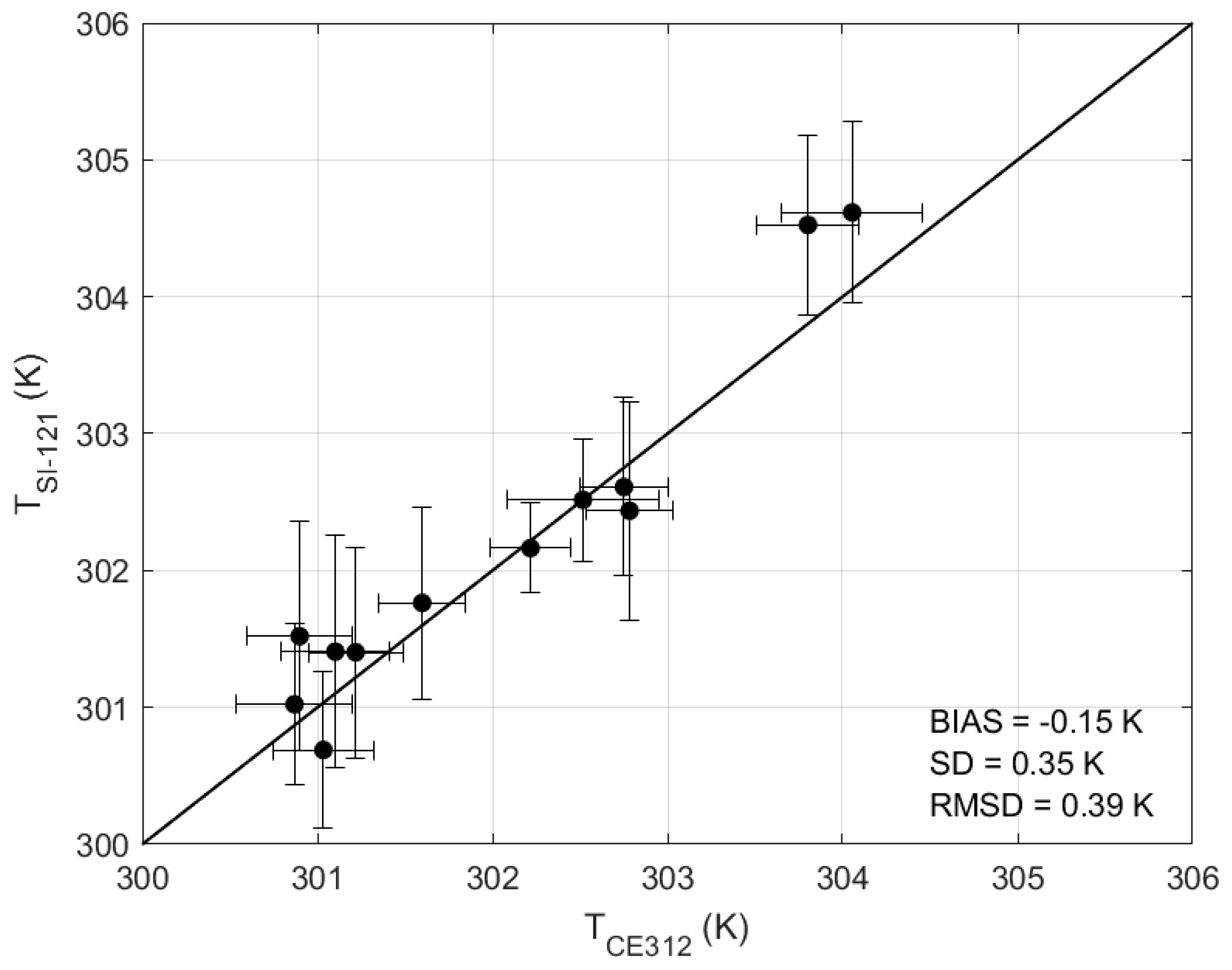
The validation used in-situ LSTs from a rice paddy site close to Valencia, Spain, which represents three seasonal homogeneous land cover types with different spectral features. These in-situ data were collected by two Apogee SI-121 wideband (8–14 µm) radiometers installed on a permanent station at the site. The narrower viewing geometry and spectral range makes TIR radiometers (e.g., Apogee SI-121, Heitronics KT15.85) more suitable for LST validation purposes than broadband hemispherical pyrgeometers (3–50 µm), which are commonly used [32]. Additionally, the uncertainty of typically used radiometers (e.g., ±0.2 K for Apogee SI-121) is lower than for pyrgeometers, which is around 1 K [60]. When considering the uncertainties in upwelling and downwelling radiance measurements and emissivity, the uncertainty of in-situ LST obtained with pyrgeometers results in a typical uncertainty of ±1 to ±2 K [61]. In [62], compared simultaneous measurements with wideband radiometers and a pyrgeometer over asphalt and four grassland sites. From this comparison, they observed a standard deviation of up to 2 K at the grassland sites and a general underestimation for the pyrgeometer data. This is in agreement with LST validations performed for various satellite sensors, e.g., MODIS [63], VIIRS [60], and Landsat-8 [64], which used pyrgeometer measurements as reference: especially at daytime, these studies obtained similar standard deviations of around 2 K at grassland sites.

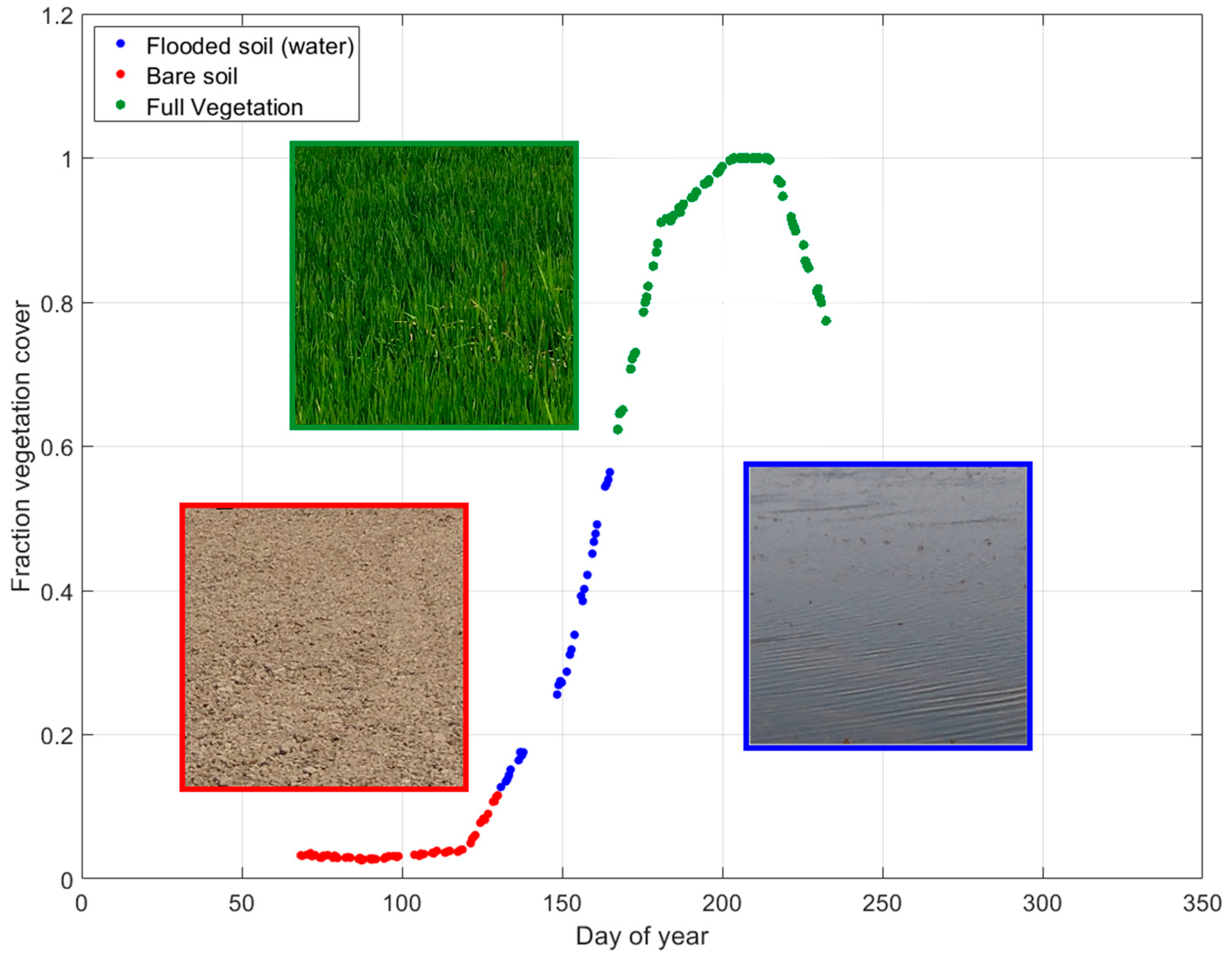
The GlobCover classification map, which is based on a static global classification, is used for generating the SLSTR LST product. In order to consider surface changes due to vegetation, seasonal changes or cropland harvest, each coefficient of the operational SLSTR LST algorithm is obtained as a combination of a vegetation coefficient and a bare soil coefficient, weighted by their cover fractions. However, for flooded soil at the study site, the vegetation fraction is higher than 0.3 (Figure 2): while this may be plausible for the last few days considered as flooded soil, when the rice starts growing, it is implausible at the beginning of the flooding, when there is only water. According to agricultural laborers, changes on the surface should be more marked, since the site is flooded in a few days and is then covered entirely by water. However, for 15 out of 27 land cover types, the vegetation and bare soil coefficients provided in the SLSTR auxiliary data are the same, as is the case for the biome assigned to the study site (i.e., weighting by cover fraction has no effect).

Different coefficients for daytime and nighttime are provided only for water and flooded surface biomes (i.e., post-flooding or irrigated cropland). However, for most land cover types, e.g., bare soils, non-flooded forests, scrubland or grassland areas, the coefficients are the same for daytime and nighttime.

In the SLSTR LST algorithm, coefficients for irrigated cropland areas were obtained as an average of the coefficients for water, winter wheat, and broadleaf-deciduous trees according to the land cover classification given in [65]. Since the land cover of the study site changes over the year, only the period of full vegetation matches with the assigned biome. However, the best validation results were obtained for the bare soil cover at daytime (R-RMSD = 1.6 K) and nighttime (R-RMSD = 1.0 K). Similar results were obtained for the SLSTR LST product over arid areas by other authors. In [20], a RMSD of 1.9 K at the Gobabeb (Namibia) station was obtained, with a bias of 1.8 K and a SD of 0.8 K. In [23], a bias of 1.1 K and a SD of 0.9 K were obtained, leading to a RMSD of 1.4 K. In these two cases, as well as in this study, SLSTR LST had a good precision, i.e., lower than or equal to 1.0 K, but an accuracy larger than the GCOS threshold (>1 K). Yang et al. in [49] obtained a systematic uncertainty of 1.6 K and a RMSD of 2.4 K for Sentinel-3 SLSTR LST at the Gobabeb (Namibia) site. It should be noted that the biomes assigned to each validation site differ, so discrepancies due to different coefficients are possible.

For the Valencia rice paddy site, the validation over full vegetation cover shows considerably better results at nighttime, with median and RSD around 1K. However, for the daytime data, the median and RSD increase to 1.7 and 1.5 K, respectively. Due to the higher thermal heterogeneity at daytime, a slight increase in RSD is expected, but not the large increase observed for the median difference, which causes the daytime accuracy to miss the GCOS threshold. It is suspected that the increased median difference is mainly caused by different day and night retrieval coefficients. These results cannot be directly compared with results obtained over other vegetated areas, e.g., the Amazon site [48] and Evora [20]. The Amazon site [48] was classified as closed to open broadleaved evergreen and/or semi-deciduous forest (biome 5) and yielded a SLSTR LST bias of −0.1 and a SD of 0.6 K for daytime and nighttime data. For Evora [20], the assigned biome was rainfed croplands (biome 2) and the SLSTR LST bias was −0.8 (−0.4) K and SD 0.7 (0.3) K for daytime (nighttime). The biases obtained for these validation sites were relatively small and showed a slight LST underestimation, while an overestimation was found at the Valencia site, which was misclassified as biome 1 (irrigated cropland) with very different characteristics to a rice paddy.

For the evaluation of the operational Sentinel-3B SLSTR product, a total of 107 scenes (43 over flooded soil, 31 over bare soil, and 28 over full vegetation) were used. Compared to the validation results for Sentinel-3A, the obtained accuracy for full vegetation and bare soil was slightly better, while the precision was similar for full vegetation and worse for bare soil. For flooded soil, the validation results for Sentinel-3B were less accurate and more precise than for Sentinel-3A. As for Sentinel-3A, better results were observed for Sentinel-3B nighttime data, mainly because of the higher thermal homogeneity. For both sensors, large systematic uncertainty was observed over flooded soil (around 2 K for both daytime and nighttime). In contrast, over the deep and large water body of Lake Constance (classified as water body, biome 26), Yang et al. in [49] reported a considerably smaller systematic uncertainty of 0.4 K and a RMSD of 0.7 K for the operational Sentinel-3 SLSTR LST product.

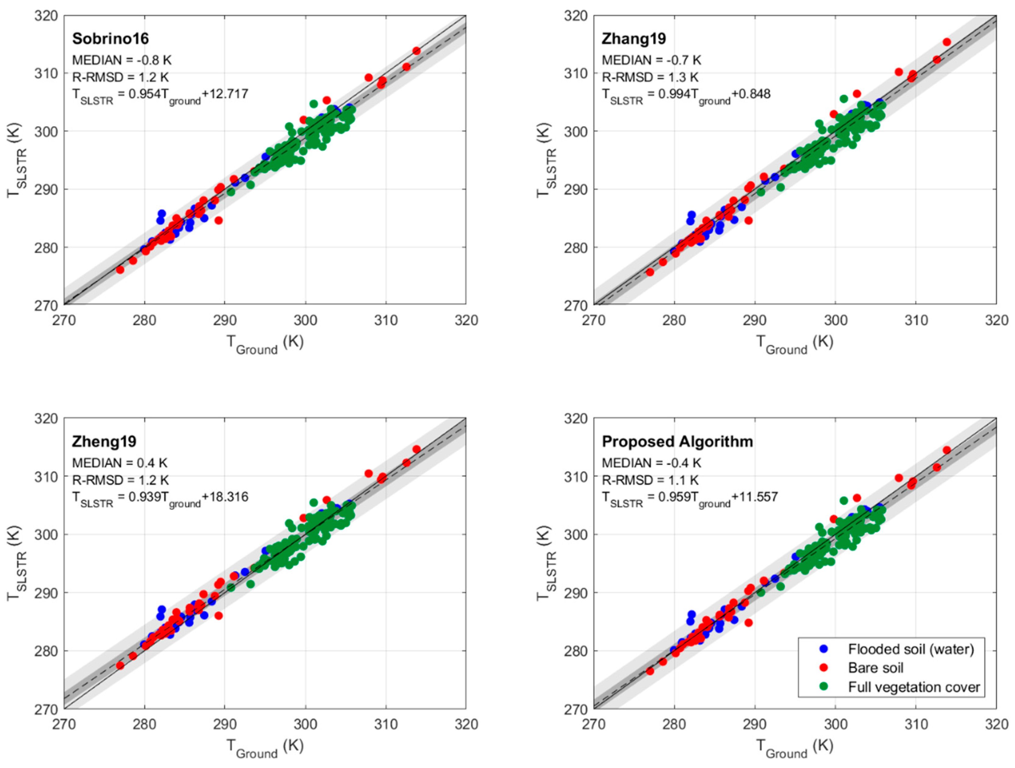
The proposed SWA with explicit emissivity and angular dependence and the three published emissivity-dependent SWAs were validated under identical conditions. Generally, all investigated algorithms performed well, with median and RSD lower than 1.5 K over all surfaces. For all surfaces combined, the proposed algorithm yielded median (RSD) values of −0.4 K (1.1 (K): together with the Zheng19 SWA, it showed the lowest median (best accuracy). However, all SWAs obtained similar RSD values between 0.9 and 1.1 K. The better accuracy of the Zheng19 algorithm is mainly linked to its exceptionally low median over full vegetation cover, which also represented most data; the other SWA proposed here showed more consistently low median values for all three land covers.

The coefficients of the proposed SWA were based on a simulated dataset produced for LST ranging between −6 K and +12 K around the lowest level of air temperature (T₀). These values were determined in [50] from statistical analysis of MODIS products MOD08 and MOD11 for air temperature and LST values, respectively. This statistical analysis showed that the range of temperatures used for the simulation dataset covers most of the cases found over natural surfaces [50]. A maximum increment of up to +20 K was used to produce Sobrino16 and Zhang19, although these increments were only for T₀ < 280 K on the latter. The Zheng19 SWA was produced with even larger increments of up to +30 K: this can be interesting for some applications (e.g., urban heat island, analyses of extreme temperatures), but can also cause an overfitting of retrieval coefficients, which in turn can increase retrieval uncertainty, particularly over the most common natural surfaces [64].

The similarity of the results could be linked to the moderate WVCs at the site (ranging from 0.5 to 4.4 cm, with a mean value of 2.4 ± 0.9 cm and only 3% of data >4 cm), which implies small atmospheric effects and a small dependence on viewing angle. The effect of the differential absorption in the atmosphere in the regression of the proposed SWA per viewing angle was shown in Figure 4. For low to moderate brightness temperature differences, there is a minor angular dependence of the regression coefficients. However, for high brightness temperature differences, there is considerable angular dependence of the coefficients, corresponding to high WVCs (up to 7 cm) in the CLAR atmospheric database used for the regressions (brightness temperature differences were up to 6.4 K). For comparison, the largest values in the database for the brightness temperature difference in SLSTR channels 8 and 9 were around 4.0 K (with a mean of 1.5 ± 0.8 K). Thus, further validation experiments in tropical atmospheres and over regions with WVCs exceeding 4 cm should be performed to evaluate the algorithms in such extreme cases. Although there is a slight WVC seasonality (i.e., higher in the summer, lower in the winter), no significant differences observed in the results were unrelated to WVC, since no extreme WVC values were found at the site. Moreover, the uncertainty introduced by WVC (~0.1 K) on the SWA is negligible compared to the uncertainty introduced by emissivity (~0.5 K) or the retrieval algorithm (~1.4 K), as shown in Table 3. The difference in the accuracy obtained with the proposed SWA for viewing angles lower and higher than 40° was 0.3 K, with an associated difference in precision of 0.6 K. Based on the simulations shown in Figure 4, a decrease of precision with viewing angle was expected, since the atmospheric absorption increases considerably with viewing angle and, thus, also, the regression error. However, the relatively small change in accuracy indicates a good performance of the algorithm also at larger viewing angles.

At nighttime, for the three land covers at the rice paddy site, the algorithms showed good performance with accuracies and precisions better than the GCOS threshold (<1 K). In contrast, at daytime, the larger thermal heterogeneity caused an increase of RSDs for bare soil and full vegetation covers, with values of about 1.5 K. However, generally, similar accuracies were obtained at daytime and nighttime over bare soil and full vegetation cover and most values met the GCOS accuracy threshold.

For all algorithms the results were in agreement with previous validations performed by other authors at different sites: in [21] obtained a bias of −1.4 K and a SD of 1.2 K for a cropland area in Oklahoma, which is comparable to our site with full vegetation cover. Although they had few data points, their results showed a similar precision to that obtained for the rice paddy site. Similar results were also obtained for SLSTR LST at an Amazon site in [48], who obtained a bias of −1.3 K and a SD of 0.9 K. Zhang et al. in [22] obtained a bias of −0.4 K and a SD of 0.9 K for a desert area in Wuhai, which are similar results to those obtained here with the same algorithm for bare soil. Yang et al. in [49] trained nine SWAs to retrieved SLSTR LST. These SWAs were evaluated over the gravel plains at Gobabeb (Namibia) and Lake Constance (Germany, Switzerland and Austria); a bias from −0.2 K to −0.3 K (from −0.2 K to 0.3 K) and an RMSD of 1.6 K (0.5 K) were obtained at Gobabeb (Lake Constance). Finally, Zheng et al. in [23] validated their proposed SWA using pyrgeometers and radiometers over cropland and grassland sites. Their overall results showed a bias of 0.6 K and SD of 2.2 K, which is higher than the corresponding values obtained at our study site for all surfaces combined and for full vegetation cover. The underestimation reported for a station at Henan Hebi, China, with daytime data from a radiometer over cropland, was similar to that for vegetation cover at our site, under similar conditions. 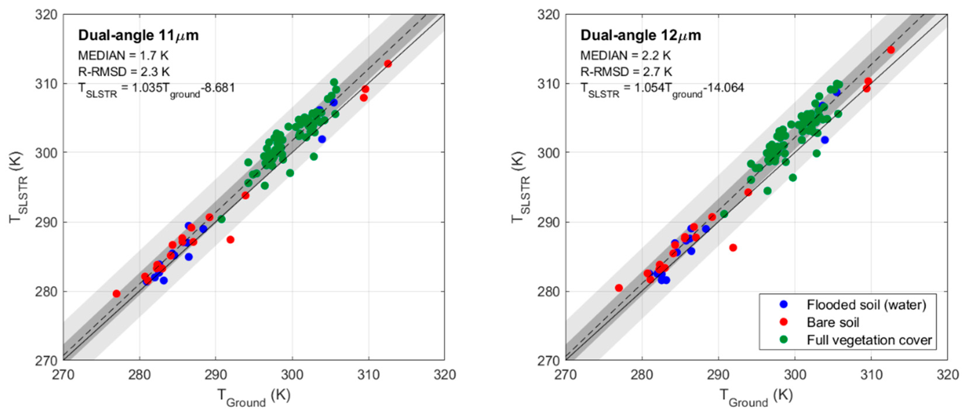The bias obtained in [23] was the same as the median obtained here, while SD deviation was 2.4 K at the Henan Hebi site. The RSD found here was 1.3 K and, therefore, the Zheng19 algorithm performed much better at our study site. The proposed DAAs, which use SLSTR’s nadir and backward views, showed better results for the version applied to the 11 µm channel (DAA11), which over flooded soil yielded an accuracy and precision better than the GCOS threshold. For bare soil, the accuracy and precision were also close to the GCOS threshold. However, the accuracy was worse for full vegetation cover. DAA12 yielded R-RMSD values between 1.8 and 3 K for all land covers. These findings are in agreement with results for previous sensors (i.e., AATSR, [16,50]), where, regardless of land cover, DAAs also performed worse than SWAs, probably due to differences in sensor footprint between the views and directional effects on radiometric temperatures [16].

6. Conclusions

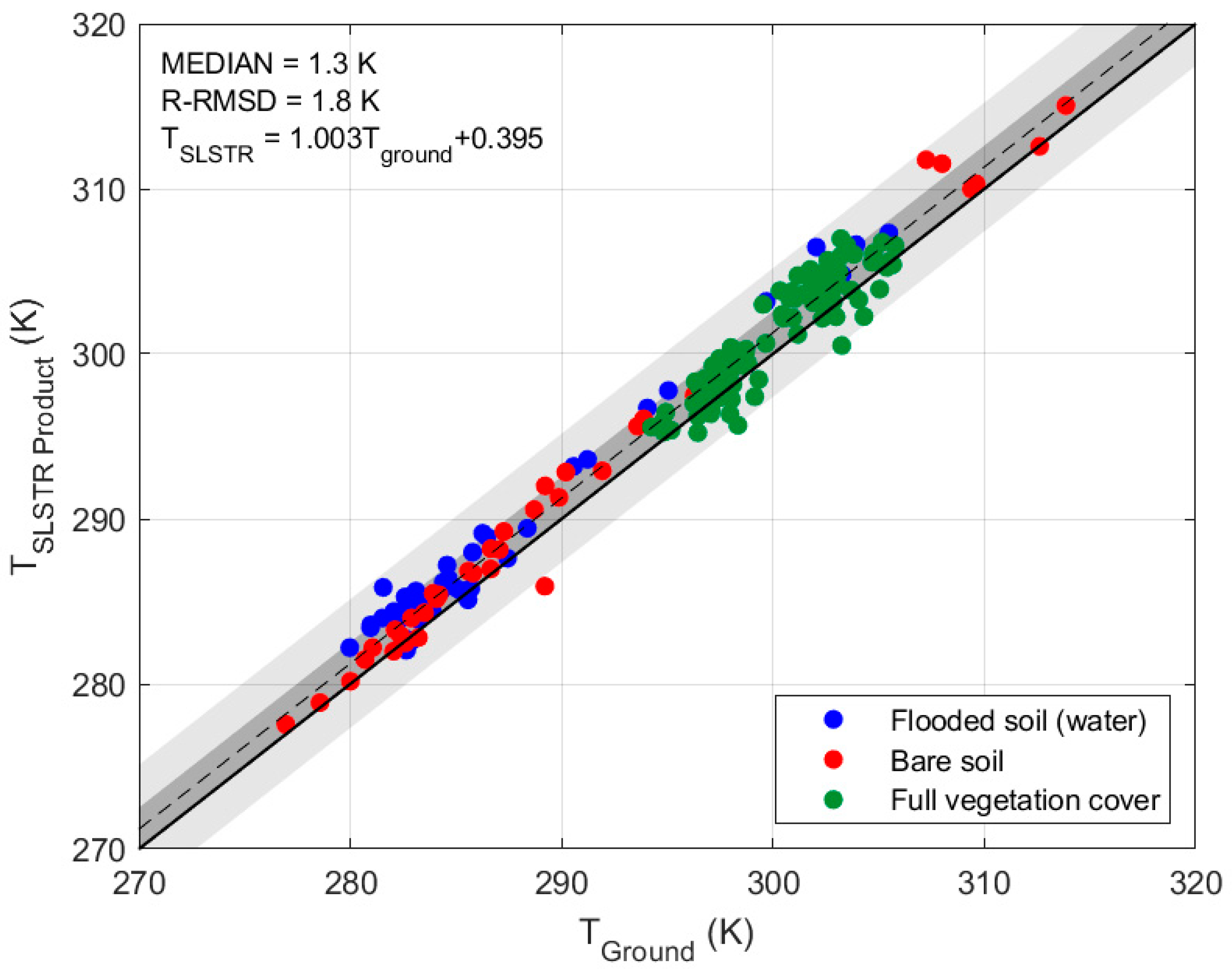
The operational SLSTR LST algorithm depends on biome, day/nighttime, vegetation fraction, and viewing zenith angle. From the validation results it is concluded that the operational Sentinel-3A SLSTR LST product is accurate for nighttime data, with an accuracy (systematic uncertainty, i.e., median) of 1.0 K and a precision (random uncertainty, i.e., RSD) of 1.0 K for the three investigated surfaces combined. In contrast, for daytime data an accuracy of 1.8 K and precision 1.2 K was determined. The increase in daytime RSD is attributed to the typically larger thermal heterogeneity of the land surface. In contrast, the increase in bias is thought to be caused by wrongly assigned biomes, i.e., the same coefficients were used for the three investigated land cover types. Additionally, the validation for the Sentinel-3B SLSTR LST product is of relevance since no robust validations were published for this platform. An accuracy of 1.5 K and a precision of 1.2 K were obtained, yielding to similar results to those obtained for the Sentinel-3A SLSTR LST product for all data combined.

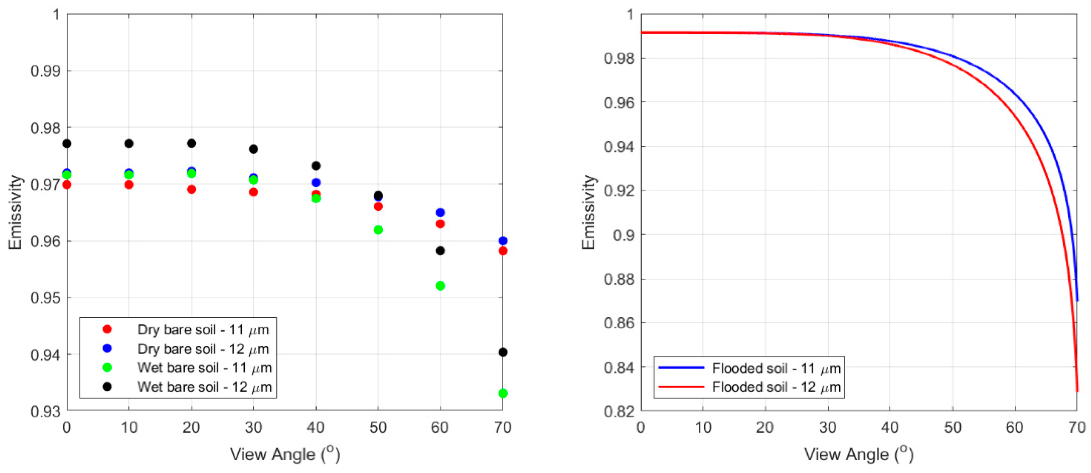
The angular and emissivity-dependent algorithm proposed by Niclòs et al. in [15] for MSG SEVIRI was adapted to Sentinel-3 SLSTR. The adapted SLSTR SWA was evaluated together with three emissivity-dependent algorithms proposed by Sobrino et al. in [21], Zhang et al. in [22] and Zheng et al. in [23] using Sentinel-3A SLSTR L1 data. For all data combined (i.e., the three land cover types), the differences between LST obtained with the proposed algorithm and in-situ LST had a median (RSD) of −0.4 K (1.1 K); the respective values were −0.8 K (0.9 K) for Sobrino16, −0.7 K (1.1 K) for Zhang19, and 0.4 K (1.1 K) for Zheng19. While Zheng19 and the SWA proposed here achieved the overall best accuracies, the latter showed a more consistent performance for the three investigated land covers. These cover a wide range of natural surface emissivities, i.e., from low values for dry bare soil, to medium values for wet bare soil, and high emissivity values for vegetation and water surfaces. Additionally, the explicit angular dependence of the proposed SWA will have higher benefits over areas with higher WVC, which is also illustrated by simulation data).

The overall accuracy improvements of the proposed SWA compared to the operational product is of 0.9 K, while it is 0.4 and 0.3 K compared to Sobrino16 and Zhang19 SWAs, respectively. The achieved improvements are highly significant, e.g., for climatological studies: when performing LST trend analyses, a global LST increase of 0.27 K/decade was observed from satellite data [66], i.e., the observed trends per decade are still smaller than the accuracy improvement achieved by the proposed algorithm.

Furthermore, a DAA was proposed to investigate the usefulness of SLSTR’s dual-view capability for LST retrieval and separate sets of coefficients were determined for the 11 and 12 µm channels. While DAA11 performed better than DAA12, the dual-view algorithms still performed worse than the SWAs. However, an acceptable accuracy and precision of DAA11 was found over flooded soil and bare soil at the Valencia rice paddy site.

Over the rice paddy site, the explicitly emissivity-dependent SWAs were found to perform better than the operational Sentinel-3 SLSTR algorithm with biome-dependent coefficients. Among the emissivity-dependent SWAs, the proposed algorithm with explicit angular dependence showed a slightly better performance at the three land covers. The results of this algorithm are expected to improve for more humid atmospheres (i.e., WCV > 4 cm), where the impact of the angular effect is higher due to the increased atmospheric absorption.

References

1. Sánchez, J.M.; López-Urrea, R.; Dona, C.; Caselles, V.; González-Piqueras, J.; Niclos, R. Modeling evapotranspiration in a spring wheat from thermal radiometry: Crop coefficients and E/T partitioning. Irrig. Sci. 2015, 33, 399–410. [Google Scholar] [CrossRef]
2. Mokhtari, A.; Noory, H.; Pourshakouri, F.; Haghighatmehr, P.; Afrasiabian, Y.; Razavi, M.; Fereydooni, F.; Naeni, A.S. Calculating potential evapotranspiration and single crop coefficient based on energy balance equation using Landsat 8 and Sentinel. ISPRS J. Photogramm. Remote Sens. 2019, 154, 231–245. [Google Scholar] [CrossRef]
3. Bian, Z.; Roujean, J.-L.; Lagouarde, J.-P.; Cao, B.; Li, H.; Du, Y.; Liu, Q.; Xiao, Q.; Liu, Q. A semi-empirical approach for modeling the vegetation thermal infrared directional anisotropy of canopies based on using vegetation indices. ISPRS J. Photogramm. Remote Sens. 2020, 160, 136–148. [Google Scholar] [CrossRef]
4. Li, Z.-L.; Tang, B.-H.; Wu, H.; Ren, H.; Yan, G.; Wan, Z.; Trigo, I.; Sobrino, J.A. Satellite-derived land surface temperature: Current status and perspectives. Remote Sens. Environ. 2013, 131, 14–37. [Google Scholar] [CrossRef] [Green Version]
5. Csiszar, I.; Schroeder, W.; Giglio, L.; Ellicott, E.; Vadrevu, K.P.; Justice, C.O.; Wind, B. Active fires from the Suomi NPP Visible Infrared Imaging Radiometer Suite: Product status and first evaluation results. J. Geophys. Res. Atmos. 2014, 119, 803–816. [Google Scholar] [CrossRef]
6. Wang, J.; Roudini, S.; Hyer, E.J.; Xu, X.; Zhou, M.; Garcia, L.C.; Reid, J.S.; Peterson, D.A.; da Silva, A.M. Detecting nighttime fire combustion phase by hybrid application of visible and infrared radiation from Suomi NPP VIIRS. Remote Sens. Environ. 2020, 237, 111466. [Google Scholar] [CrossRef]
7. Cigna, F.; Tapete, D.; Lu, Z. Remote Sensing of Volcanic Processes and Risk. Remote Sens. 2020, 12, 2567. [Google Scholar] [CrossRef]
8. Nádudvari, Á.; Abramowicz, A.; Maniscalco, R.; Viccaro, M. The Estimation of Lava Flow Temperatures Using Landsat Night-Time Images: Case Studies from Eruptions of Mt. Etna and Stromboli (Sicily, Italy), Kīlauea (Hawaii Island), and Eyjafjallajökull and Holuhraun (Iceland). Remote Sens. 2020, 12, 2537. [Google Scholar] [CrossRef]
9. Gerhards, M.; Schlerf, M.; Mallick, K.; Udelhoven, T. Challenges and Future Perspectives of Multi-/Hyperspectral Thermal Infrared Remote Sensing for Crop Water-Stress Detection: A Review. Remote Sens. 2019, 11, 1240. [Google Scholar] [CrossRef] [Green Version]
10. Hatton, N.; Sharda, A.; Schapaugh, W.; van der Merwe, D. Remote thermal infrared imaging for rapid screening of sudden death syndrome in soybean. Comput. Electron. Agric. 2020, 178, 105738. [Google Scholar] [CrossRef]
11. Chang, S.; Chen, H.; Wu, B.; Nasanbat, E.; Yan, N.; Davdai, B. A Practical Satellite-Derived Vegetation Drought Index for Arid and Semi-Arid Grassland Drought Monitoring. Remote Sens. 2021, 13, 414. [Google Scholar] [CrossRef]
12. GCOS. The Global Observing System for Climate: Implementation Needs. World Meteorol. Organ. 2016, 200, 341. Available online: https://library.wmo.int/opac/doc_num.php?explnum_id=3417 (accessed on 1 May 2021).
13. Hollmann, R.; Merchant, C.J.; Saunders, R.; Downy, C.; Buchwitz, M.; Cazenave, A.; Chuvieco, E.; Defourny, P.; De Leeuw, G.; Forsberg, R.; et al. The ESA Climate Change Initiative: Satellite Data Records for Essential Climate Variables. Bull. Am. Meteorol. Soc. 2013, 94, 1541–1552. [Google Scholar] [CrossRef] [Green Version]
14. Lequin, R.M. Guide to the Expression of Uncertainty of Measurement: Point/Counterpoint. Clin. Chem. 2004, 50, 977–978. [Google Scholar] [CrossRef] [PubMed]
15. Niclòs, R.; Galve, J.M.; Valiente, J.A.; Estrela, M.J.; Coll, C. Accuracy assessment of land surface temperature retrievals from MSG2-SEVIRI data. Remote Sens. Environ. 2011, 115, 2126–2140. [Google Scholar] [CrossRef]
16. Coll, C.; Caselles, V.; Galve, J.M.; Valor, E.; Niclòs, R.; Sánchez, J.M. Evaluation of split-window and dual-angle correction methods for land surface temperature retrieval from Envisat/Advanced Along Track Scanning Radiometer (AATSR) data. J. Geophys. Res. Space Phys. 2006, 111, 1–12. [Google Scholar] [CrossRef] [Green Version]
17. Fisher, D.; Wooster, M.J. Multi-decade global gas flaring change inventoried using the ATSR-1, ATSR-2, AATSR and SLSTR data records. Remote Sens. Environ. 2019, 232, 111298. [Google Scholar] [CrossRef]
18. Ghent, D.J.; Corlett, G.K.; Göttsche, F.-M.; Remedios, J.J. Global Land Surface Temperature from the Along-Track Scanning Radiometers. J. Geophys. Res. Atmos. 2017, 122, 12–167. [Google Scholar] [CrossRef] [Green Version]
19. Sentinel-3 Optical Products and Algorithm Definition: SLSTR Land Surface Temperarure Algorithm Theoretical Basis Document (ATBD). 2012. Available online: https://sentinel.esa.int/documents/247904/349589/SLSTR_Level-2_LST_ATBD.pdf (accessed on 1 May 2021).
20. Ghent, D. S3 Validation Report—SLSTR. Internal Publication, S3MPC.UOL.VR.029 Issue 1.0, 65p. Available online: https://sentinels.copernicus.eu/documents/247904/3320896/Sentinel-3-SLSTR-Level-2-Land-Validation-Report (accessed on 1 May 2021).
21. Sobrino, J.; Jiménez-Muñoz, J.; Sòria, G.; Ruescas, A.; Danne, O.; Brockmann, C.; Ghent, D.; Remedios, J.; North, P.; Merchant, C.; et al. Synergistic use of MERIS and AATSR as a proxy for estimating Land Surface Temperature from Sentinel-3 data. Remote Sens. Environ. 2016, 179, 149–161. [Google Scholar] [CrossRef]
22. Zhang, S.; Duan, S.-B.; Li, Z.-L.; Huang, C.; Wu, H.; Han, X.-J.; Leng, P.; Gao, M. Improvement of Split-Window Algorithm for Land Surface Temperature Retrieval from Sentinel-3A SLSTR Data Over Barren Surfaces Using ASTER GED Product. Remote Sens. 2019, 11, 3025. [Google Scholar] [CrossRef] [Green Version]
23. Zheng, Y.; Ren, H.; Guo, J.; Ghent, D.; Tansey, K.; Hu, X.; Nie, J.; Chen, S. Land Surface Temperature Retrieval from Sentinel-3A Sea and Land Surface Temperature Radiometer, Using a Split-Window Algorithm. Remote Sens. 2019, 11, 650. [Google Scholar] [CrossRef] [Green Version]
24. Miralles, V.C.; Valor, E.; Boluda, R.; Caselles, V.; Coll, C. Influence of soil water content on the thermal infrared emissivity of bare soils: Implication for land surface temperature determination. J. Geophys. Res. Space Phys. 2007, 112, 1–11. [Google Scholar] [CrossRef] [Green Version]
25. Coll, C.; Galve, J.M.; Sanchez, J.M.; Caselles, V. Validation of Landsat-7/ETM+ Thermal-Band Calibration and Atmospheric Correction With Ground-Based Measurements. IEEE Trans. Geosci. Remote Sens. 2010, 48, 547–555. [Google Scholar] [CrossRef]
26. Coll, C.; Garcia-Santos, V.; Niclos, R.; Caselles, V. Test of the MODIS Land Surface Temperature and Emissivity Separation Algorithm With Ground Measurements Over a Rice Paddy. IEEE Trans. Geosci. Remote Sens. 2016, 54, 3061–3069. [Google Scholar] [CrossRef]
27. Niclòs, R.; Pérez-Planells, L.; Coll, C.; Valiente, J.A.; Valor, E. Evaluation of the S-NPP VIIRS land surface temperature product using ground data acquired by an autonomous system at a rice paddy. ISPRS J. Photogramm. Remote Sens. 2018, 135, 1–12. [Google Scholar] [CrossRef]
28. Niclòs, R.; Puchades, J.; Coll, C.; Barberà, M.J.; Pérez-Planells, L.; Valiente, J.A.; Sánchez, J.M. Evaluation of Landsat-8 TIRS data recalibrations and land surface temperature split-window algorithms over a homogeneous crop area with different phenological land covers. ISPRS J. Photogramm. Remote Sens. 2021, 174, 237–253. [Google Scholar] [CrossRef]
29. Coll, C.; Caselles, V.; Galve, J.; Valor, E.; Niclos, R.; Sanchez, J.; Rivas, R. Ground measurements for the validation of land surface temperatures derived from AATSR and MODIS data. Remote Sens. Environ. 2005, 97, 288–300. [Google Scholar] [CrossRef]
30. Coll, C.; Caselles, V.; Valor, E.; Niclos, R.; Sánchez, J.M.; Galve, J.M.; Mira, M. Temperature and emissivity separation from ASTER data for low spectral contrast surfaces. Remote Sens. Environ. 2007, 110, 162–175. [Google Scholar] [CrossRef]
31. Niclòs, R.; Valiente, J.A.; Barberà, M.J.; Coll, C. An Autonomous System to Take Angular Thermal-Infrared Measurements for Validating Satellite Products. Remote Sens. 2015, 7, 15269–15294. [Google Scholar] [CrossRef] [Green Version]
32. Guillevic, P.; Göttsche, F.; Nickeson, J.; Hulley, G.; Ghent, D.; Yu, Y.; Trigo, I.; Hook, S.; Sobrino, J.A.; Remedios, J.; et al. Land Surface Temperature Product Validation Best Practice Protocol, Version 1.1.; National Aeronautics and Space Administration: Washington, DC, USA, 2018; p. 58. [CrossRef]
33. Theocharous, E.; IBarker Snook, I.; Fox, N.P. 2016 Comparison of IR Brightness Temperature Measurements in Support of Satellite Validation Part 1; Blackbody Laboratory Comparison: Teddington, UK, 2017. [Google Scholar]
34. Coll, C.; Niclòs, R.; Puchades, J.; García-Santos, V.; Galve, J.M.; Pérez-Planells, L.; Valor, E.; Theocharous, E. Laboratory calibration and field measurement of land surface temperature and emissivity using thermal infrared multiband radiometers. Int. J. Appl. Earth Obs. Geoinf. 2019, 78, 227–239. [Google Scholar] [CrossRef]
35. Legrand, M.; Pietras, C.; Brogniez, G.; Haeffelin, M.; Abuhassan, N.K.; Sicard, M. A High-Accuracy Multiwavelength Radiometer for In Situ Measurements in the Thermal Infrared. Part I: Characterization of the Instrument. J. Atmos. Ocean. Technol. 2000, 17, 1203–1214. [Google Scholar] [CrossRef]
36. Garcia-Santos, V.; Valor, E.; Caselles, V.; Mira, M.; Galve, J.M.; Coll, C. Evaluation of Different Methods to Retrieve the Hemispherical Downwelling Irradiance in the Thermal Infrared Region for Field Measurements. IEEE Trans. Geosci. Remote Sens. 2012, 51, 2155–2165. [Google Scholar] [CrossRef]
37. Vanhellemont, Q. Combined land surface emissivity and temperature estimation from Landsat 8 OLI and TIRS. ISPRS J. Photogramm. Remote Sens. 2020, 166, 390–402. [Google Scholar] [CrossRef]
38. Cao, B.; Guo, M.; Fan, W.; Xu, X.; Peng, J.; Ren, H.; Du, Y.; Li, H.; Bian, Z.; Hu, T.; et al. A New Directional Canopy Emissivity Model Based on Spectral Invariants. IEEE Trans. Geosci. Remote Sens. 2018, 56, 6911–6926. [Google Scholar] [CrossRef] [Green Version]
39. Ren, H.; Yan, G.; Chen, L.; Li, Z. Angular effect of MODIS emissivity products and its application to the split-window algorithm. ISPRS J. Photogramm. Remote Sens. 2011, 66, 498–507. [Google Scholar] [CrossRef]
40. Gillespie, A.; Rokugawa, S.; Matsunaga, T.; Cothern, J.; Hook, S.; Kahle, A. A temperature and emissivity separation algorithm for Advanced Spaceborne Thermal Emission and Reflection Radiometer (ASTER) images. IEEE Trans. Geosci. Remote Sens. 1998, 36, 1113–1126. [Google Scholar] [CrossRef]
41. Garcia-Santos, V.; Valor, E.; Caselles, V.; Coll, C.; Burgos, M.A. Effect of Soil Moisture on the Angular Variation of Thermal Infrared Emissivity of Inorganic Soils. IEEE Geosci. Remote Sens. Lett. 2014, 11, 1091–1095. [Google Scholar] [CrossRef] [Green Version]
42. Rubio, E. Emissivity measurements of several soils and vegetation types in the 8–14, μm Wave band: Analysis of two field methods. Remote Sens. Environ. 1997, 59, 490–521. [Google Scholar] [CrossRef]
43. Rubio, E.; Caselles, V.; Coll, C.; Valour, E.; Sospedra, F. Thermal–infrared emissivities of natural surfaces: Improvements on the experimental set-up and new measurements. Int. J. Remote Sens. 2003, 24, 5379–5390. [Google Scholar] [CrossRef]
44. Bock, O.; Keil, C.; Richard, E.; Flamant, C.; Bouin, M.-N. Validation of precipitable water from ECMWF model analyses with GPS and radiosonde data during the MAP SOP. Q. J. R. Meteorol. Soc. 2005, 131, 3013–3036. [Google Scholar] [CrossRef]
45. Dyroff, C.; Zahn, A.; Christner, E.; Forbes, R.; Tompkins, A.M.; Van Velthoven, P.F.J. Comparison of ECMWF analysis and forecast humidity data with CARIBIC upper troposphere and lower stratosphere observations. Q. J. R. Meteorol. Soc. 2015, 141, 833–844. [Google Scholar] [CrossRef]
46. Ovarlez, J.; Van Velthoven, P.; Sachse, G.; Vay, S.; Schlager, H.; Ovarlez, H. Comparison of water vapor measurements from POLINAT 2 with ECMWF analyses in high-humidity conditions. J. Geophys. Res. Space Phys. 2000, 105, 3737–3744. [Google Scholar] [CrossRef]
47. Bicheron, P.; Defourny, P.; Brockmann, C.; Schouten, L.; Vancutsem, C.; Huc, M.; Bontemps, S.; Leroy, M.; Achard, F.; Herold, M.; et al. GLOBCOVER 2009 Products Description and Validation Report; MEDIAS-France: Touluse, France, 2011. [Google Scholar] [CrossRef]
48. Jimenez, J.C.; Gomis-Cebolla, J.; Sabrino, J.A.; Soria, G.; Skokovic, D.; Julien, Y.; Garcia-Monteiro, S.; Mattar, C.; Santamaria-Artigas, A.; Pasapera-Gonzales, J.J. Sentinel 2 and 3 for Temperature Monitoring Over the Amazon. IEEE Int. Geosci. Remote Sens. Sympos. 2018, 2–3, 5925–5928. [Google Scholar] [CrossRef]
49. Yang, J.; Zhou, J.; Göttsche, F.-M.; Long, Z.; Ma, J.; Luo, R. Investigation and validation of algorithms for estimating land surface temperature from Sentinel-3 SLSTR data. Int. J. Appl. Earth Obs. Geoinf. 2020, 91, 102136. [Google Scholar] [CrossRef]
50. Galve, J.M.; Coll, C.; Caselles, V.; Valor, E. An Atmospheric Radiosounding Database for Generating Land Surface Temperature Algorithms. IEEE Trans. Geosci. Remote Sens. 2008, 46, 1547–1557. [Google Scholar] [CrossRef]
51. Coll, C.; Caselles, V.; Sobrino, J.A.; Valor, E. On the atmospheric dependence of the split-window equation for land surface temperature. Int. J. Remote Sens. 1994, 15, 105–122. [Google Scholar] [CrossRef]
52. Coll, C.; Caselles, V. A split-window algorithm for land surface temperature from advanced very high resolution radiometer data: Validation and algorithm comparison. J. Geophys. Res. Space Phys. 1997, 102, 16697–16713. [Google Scholar] [CrossRef]
53. Donlon, C.; Berruti, B.; Buongiorno, A.; Ferreira, M.-H.; Féménias, P.; Frerick, J.; Goryl, P.; Klein, U.; Laur, H.; Mavrocordatos, C.; et al. The Global Monitoring for Environment and Security (GMES) Sentinel-3 mission. Remote Sens. Environ. 2012, 120, 37–57. [Google Scholar] [CrossRef]
54. Ghent, D.; Veal, K.; Trent, T.; Dodd, E.; Sembhi, H.; Remedios, J. A New Approach to Defining Uncertainties for MODIS Land Surface Temperature. Remote Sens. 2019, 11, 1021. [Google Scholar] [CrossRef] [Green Version]
55. Berk, A.; Anderson, G.P.; Acharya, P.K.; Shettle, E.P. MODTRAN5. 2.0.0 User’s Manual; Spectral Science Inc.: Burlingt, MA, USA; Air Force Res. Lab.: Hanscom, MA, USA, 2008. [Google Scholar]
56. Baldridge, A.M.; Hook, S.J.; Grove, C.I.; Rivera, G. The ASTER spectral library version 2. Remote Sens. Environ. 2009, 113, 711–715. [Google Scholar] [CrossRef]
57. Wan, Z.; Dozier, J. A generalized split-window algorithm for retrieving land-surface temperature from space. IEEE Trans. Geosci. Remote Sens. 1996, 34, 892–905. [Google Scholar] [CrossRef] [Green Version]
58. Wan, Z. New refinements and validation of the collection-6 MODIS land-surface temperature/emissivity product. Remote Sens. Environ. 2014, 140, 36–45. [Google Scholar] [CrossRef]
59. Wilrich, P.-T. Robust estimates of the theoretical standard deviation to be used in interlaboratory precision experiments. Accredi. Qual. Assur. 2007, 12, 231–240. [Google Scholar] [CrossRef]
60. Guillevic, P.C.; Biard, J.C.; Hulley, G.C.; Privette, J.L.; Hook, S.J.; Olioso, A.; Göttsche, F.M.; Radocinski, R.; Román, M.O.; Yu, Y.; et al. Validation of Land Surface Temperature products derived from the Visible Infrared Imaging Radiometer Suite (VIIRS) using ground-based and heritage satellite measurements. Remote Sens. Environ. 2014, 154, 19–37. [Google Scholar] [CrossRef]
61. Martin, M.A.; Ghent, D.; Pires, A.C.; Göttsche, F.-M.; Cermak, J.; Remedios, J.J. Comprehensive In Situ Validation of Five Satellite Land Surface Temperature Data Sets over Multiple Stations and Years. Remote Sens. 2019, 11, 479. [Google Scholar] [CrossRef] [Green Version]
62. Krishnan, P.; Meyers, T.P.; Hook, S.J.; Heuer, M.; Senn, D.; Dumas, E.J. Intercomparison of In Situ Sensors for Ground-Based Land Surface Temperature Measurements. Sensors 2020, 20, 5268. [Google Scholar] [CrossRef] [PubMed]
63. Duan, S.-B.; Li, Z.-L.; Li, H.; Göttsche, F.-M.; Wu, H.; Zhao, W.; Leng, P.; Zhang, X.; Coll, C. Validation of Collection 6 MODIS land surface temperature product using in situ measurements. Remote Sens. Environ. 2019, 225, 16–29. [Google Scholar] [CrossRef] [Green Version]
64. Gerace, A.; Kleynhans, T.; Eon, R.; Montanaro, M. Towards an Operational, Split Window-Derived Surface Temperature Product for the Thermal Infrared Sensors Onboard Landsat 8 and 9. Remote Sens. 2020, 12, 224. [Google Scholar] [CrossRef] [Green Version]
65. Dorman, J.L.; Sellers, P.J. A Global Climatology of Albedo, Roughness Length and Stomatal Resistance for Atmospheric General Circulation Models as Represented by the Simple Biosphere Model (SiB). J. Appl. Meteorol. 1989, 28, 833–855. [Google Scholar] [CrossRef] [Green Version]
66. Sobrino, J.; García-Monteiro, S.; Julien, Y. Surface Temperature of the Planet Earth from Satellite Data over the Period 2003–2019. Remote Sens. 2020, 12, 2036. [Google Scholar] [CrossRef]
Figure 1. RGB true color compositions (R-G-B 4-3-2; top) and false color compositions (R-G-B 8-4-3; bottom) for three Sentinel-2 Multispectral Instrument (MSI) scenes. The three land covers at the site are: bare soil (April, left), flooded soil, i.e., water (May, center), full vegetation (August, right). The location of the validation site is shown in the composition.
Remotesensing 13 02228 g001
Figure 2. Fraction of vegetation cover given by the SLSTR L2 product as a function of day of year. A representative photo for each land cover is also shown.
Remotesensing 13 02228 g002
Figure 3. Angular emissivity variation of the bare soil (left) and flooded soil (right) for the CE-312 channels centered on 11 and 12 µm.
Remotesensing 13 02228 g003
Figure 4. LST–T11 against T11T12 simulated from the CLAR database at the different view angles for the SLSTR SWA atmospheric coefficients retrieval. The regression functions corresponding to each angular dataset are plotted as lines in the same color as their corresponding data.
Remotesensing 13 02228 g004
Figure 5. LST obtained with the fixed SI-121 radiometer compared to LST obtained along the transects with mobile CE-312 radiometers.
Remotesensing 13 02228 g005
Figure 6. Operational Sentinel-3A SLSTR LST product against ground LST obtained from the SI-121 radiometer over the three seasonal land cover types at the Valencia rice paddy site. The dark grey and light grey shadows show 1-RSD and 3-RSD around the regression (dashed line).
Remotesensing 13 02228 g006
Figure 7. LST retrieved from Sentinel-3A with emissivity-dependent algorithms against in-situ LST obtained from the SI-121 radiometer. Top left: Sobrino16. Top right: Zhang19. Bottom left: Zheng19. Bottom right: the proposed algorithm.
Remotesensing 13 02228 g007
Figure 8. SLSTR LST retrieved with the dual-angle algorithms for the 11 µm channel (left; DAA11) and 12 µm channel (right; DAA12) against in-situ LST for the three seasonal land covers at the Valencia rice paddy site.
Remotesensing 13 02228 g008