
Making Use of 3D Models for Plant Physiognomic Analysis: A Review


Department of Mechanical Engineering, School of Food and Advanced Technology, Massey University, Palmerston North 4442, New Zealand
*
Author to whom correspondence should be addressed.
Remote Sens. 2021, 13(11), 2232; https://0-doi-org.brum.beds.ac.uk/10.3390/rs13112232
Submission received: 14 April 2021
/
Revised: 29 May 2021
/
Accepted: 31 May 2021
/
Published: 7 June 2021
(This article belongs to the Special Issue 3D Point Clouds for Agriculture Applications)
Abstract
:Use of 3D sensors in plant phenotyping has increased in the last few years. Various image acquisition, 3D representations, 3D model processing and analysis techniques exist to help the researchers. However, a review of approaches, algorithms, and techniques used for 3D plant physiognomic analysis is lacking. In this paper, we investigate the techniques and algorithms used at various stages of processing and analysing 3D models of plants, and identify their current limiting factors. This review will serve potential users as well as new researchers in this field. The focus is on exploring studies monitoring the plant growth of single plants or small scale canopies as opposed to large scale monitoring in the field.
1. Introduction
In recent years, a plethora of studies have been conducted on plant trait measurement in 3D [1,2,3]. Plant phenotyping is an important area of research for plant growth monitoring. It is implemented by a fusion of techniques, such as spectroscopy, non-destructive imaging, and high performance computing. Plant phenotyping provides vital information about plants for monitoring growth which is helpful to farmers for their decision making process. Plant phenotyping is a set of protocols and techniques used to precisely calculate plant architecture, composition, and growth at different growth stages. Popular plant traits for growth monitoring include stem height, stem diameter, leaf area, leaf length, leaf width, number of leaves or fruit on the plant, and biomass. However, the measurement of plant structure and growth parameters is difficult, tedious and mostly depends on destructive approaches. 3D modelling helps to access the complex plant architecture [4] which allows plant related information to be extracted, such as characterization of plants and their growth development. Conventionally all these elements have been evaluated by experts in this field using a subjective visual score, which can result in dissimilarity between expert judgements. Primarily, the aim of plant phenotyping is to calculate plant features precisely without subjective biases [5]. Therefore, 3D measurement techniques are potentially suitable as these allow measurement of plant traits and can accurately model plant geometry.
The range of 3D measurement methods include LiDAR, laser scanning, structured light, structure-from-motion, and time of flight sensors. Each of these methods has its own merits and demerits. All these methods produce a point cloud, in which every 3D point represents a point detected on the surface of the plant. Based on the measuring technique, the coordinates can be augmented by color information or the intensity of the reflected light. Current 2.5D techniques calculate distances from a single point of view (range images). In contrast, 3D models describe point clouds captured from different angles and views displaying various spatial levels of points and therefore demonstrate less occlusion, higher accuracy, spatial resolution, and sample density.
A detailed technical classification of 3D acquisition methods is shown in Figure 1. Active techniques use their own source of illumination for measurements and passive techniques use ambient light in the scene. Active sensing techniques are then classified into two types: triangulation-based methods and time-of-flight-based methods. Structured light (early Kinect sensor) and laser triangulation approaches are triangulation-based methods. LiDAR and time-of-flight cameras are time-of-flight-based methods. Field cameras and structure-from-motion (SfM) methods are type of passive techniques. A comparison between these techniques is given in Table 1.
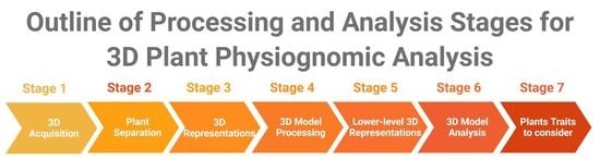
Several papers reviewed 3D image acquisition for plant phenotyping [2,6,7,8,9]. However, a review of approaches used for 3D model processing and analysis in the context of plant physiognomic analysis is lacking, which will be the focus of this review. For 3D plant model analysis, a wide set of tools is needed, because of the variety of plant architectures across species. Our aim is to identify standard processing and analysis stages, and to review techniques which have been used in each of these stages. An overview of the stages covered in this paper is shown in Figure 2.
This review addresses the questions related to 3D plant physiognomic analysis. What sensing methods can be used for such analysis? Are there any potential cost-effective and non-destructive methods? What are the various scene representations? What type of plant traits should be extracted? What are the current challenges and research directions?
2. 3D Imaging Techniques
2.1. Active Techniques
2.1.1. Laser Triangulation
Laser triangulation (LT) describes distance calculation techniques based on differing laser and sensor positions. A laser ray is transmitted to illuminate the target surface. The position of the laser spot is detected using an image sensor (see Figure 3). Since the laser and sensor are in different positions, the 3D location of the laser spot can be found through triangulation. A 3D point cloud can be generated by scanning the laser spot.
Laser triangulation has a trade-off between the target volume and point resolution. It can either measure a small target with highest possible resolution or large target with low resolution. This approach needs a prior estimation of the required resolution and the target volume. Laser triangulation is mainly used in laboratory settings because of its high accuracy, high resolution readings and easy set-up [10,11].
2.1.2. Structured Light
Structured light (SL) projects patterns, a grid, in a temporal order on the target. For every pattern an image is captured by the camera. The 2D points on the grid pattern are linked to their 3D data by calculating the distortion of the pattern (see Figure 4) [12,13]. Structured light has a bulky set-up and requires more time than other sensing techniques.
To achieve a 3D model, either the set-up or the target object has to be moved. Structured light is mostly used for industry applications to check the quality of an object, providing high accuracy and resolution [14]. The early Kinect sensor is an example of a structured light sensor.
2.1.3. Time-of-Flight
Time-of-flight (Tof) uses high frequency modulated illumination, and calculates the range from the phase shift (see Figure 5) [15]. This process can be repeated for thousands of points at the same time [5]. The set-up for Tof cameras is smaller than other methods and captures images with lower resolution. These cameras are suitable for indoor applications [16] or in the gaming industry [17]. Tof cameras are required to move in order to build a complete 3D point cloud. The cameras are slow and have low resolution, compared to laser triangulation and structure-from-motion (SfM).
2.1.4. LiDAR
LiDAR is basically an extension of the principles employed in radar technology. It calculates the distance between the scanner and the target object by illuminating the object using a laser and measuring the time taken for the reflected light to return [5]. Terrestrial LiDAR has a bulky set-up and to deal with occlusion issues, the plant has to be scanned from multiple positions. This approach has already proved its worth in surveying applications, such as landslide detection and measurement [18]. For plant growth monitoring, LiDAR has the advantage that it can measure any target volume with high accuracy. However, this approach is costly, time consuming, and bulky which makes it less suitable for plant growth monitoring.
Airborne LiDAR has also been used in some studies [19,20] to determine plant height and crown diameter measurement. Airborne LiDAR offers accurate and detailed measurements, data can be collected quickly and from a variety of locations. However, there are some limitations such as underestimation of vegetation height compared to field measurements [21,22] and it struggles with dense vegetation canopy where the dense undergrowth may be confused with bare ground. The underestimation of vegetation height is also dependent on plant species and growth stage [23].
2.2. Passive Techniques
2.2.1. Stereo Vision
Stereo vision has three main processing stages: camera calibration, feature extraction, and correspondence matching. A stereo camera captures a pair of images (right and left). Using this stereo pair, the disparity can be calculated between the camera coordinates of matching points in the scene, thus the depth can then be calculated through triangulation (see Figure 6).
2.2.2. Structure-from-Motion
Structure-from-motion (SfM) uses a set of 2D images acquired by an RGB camera at different positions to generate a 3D model of the target [24] (see Figure 7). Corresponding points in the images are extracted [25] and matched to stitch the images together and generate the 3D model. The 3D point cloud includes color and intensity information depending on the type of camera used [26].
The point resolution achieved from SfM is comparable to laser triangulation. However, it depends on the camera resolution and number of images used for 3D modelling [26].
Structure-from-motion can be used by mounting a camera on an unmanned aerial vehicle (UAV). This set-up is cheaper than airborne LiDAR. It is easy to gather data on a small study area, and overcast or partly cloudy conditions have less effect on the acquisition process. However, it is computationally demanding and it cannot penetrate the plant’s canopy.
In contrast with laser triangulation, which requires more time for acquisition and the direct result is the point cloud, SfM requires less time for acquiring the images, but needs more time for reconstruction. SfM can be used in outdoor environments as it does not require special illumination or complex set-up. This method requires only an off-the-shelf camera to capture the images, the set-up is cost-effective and easy.
2.2.3. Field Cameras
Field cameras [27] gives depth information with color image by calculating the direction of the light coming in using camera arrays. This allows the reconstruction of the target. However, similar to time-of-flight sensors, field cameras also need to move with a bulky set-up which makes them difficult in outdoor applications.
2.3. A Constructive Comparison of 3D Imaging Techniques
Active techniques provide a high-resolution point cloud for further plant analysis such as plant trait segmentation and measurement. However, the influence of the laser on plant tissue has to be considered when active illumination techniques are used, especially laser triangulation. Even though laser-based techniques are described as non-penetrating, recent studies have found that plant tissue below cuticle (protecting covering) has significant impact on the trait measurement and accuracy due to laser intensity [9]. In addition, because of the edge effect [28,29], plant trait measurements of partial leaves can generate outliers or errors in the measurement. Other active techniques such as structured light, time-of-flight, and LiDAR have proven their worth for plant phenotyping demands. However, the resolution and accuracy have to be improved for high throughput plant physiognomic analysis. Table 2 summarises the advantages and disadvantages of the various 3D imaging techniques.
In contrast, structure-from-motion gives an easy and cost-effective solution. This makes them best suited for outdoor applications. However, the resolution of the point cloud depends on the number of images captured. Additionally, SfM requires more computation time than the other methods. Summing up, SfM is a reliable technique for 3D modelling of plants while resolving occlusion, self occlusion, correspondence problems, and providing high resolution information.
In all these studies, researchers have used different sensors and techniques to derive a 3D model. In conclusion, every sensor and technique has its merits and demerits [5] and their accuracy may vary. One should choose the sensors and techniques depending on the budget and requirements [30]. However, if budget is a limiting factor, based on the comparison provided in Table 1, one must choose structure-from-motion as it is not only a cost-effective and non-destructive solution, but also it provides better point cloud resolution at the lowest price.
3. Plant Separation in Clusters and Row Structure
In some scenarios, the plants are planted in a row or in a cluster. To detect individual plants, various active and passive methods have been developed in the literature [31,32]. In particular, LiDAR has been widely used over the past decade. Due to the high spatial resolution of airborne laser scanner (ALS), its data provide important information used for individual tree detection [33,34]. In the last 20 years, many fully and semi-automatic algorithms have been developed for detection of individual plants. However, even if one algorithm is best for a specific application, it may not be ideal for other situations. For instance, some algorithms may work well on canopies with large variations in plant growth stage, plant spacing, or plant crowns with high degree of occlusion [35,36]. It is challenging to decide an ideal algorithm to detect individual plants as there is no standard method to assess the accuracy of the algorithm [37]. This section will cover the work related to LiDAR information using a canopy height model (CHM), digital surface model (DSM), and using passive methods to generate point cloud to detect the individual plants. Individual plant detection algorithms are grouped into four categories by Koch et al. [38]: (1) raster-based algorithms; (2) point cloud-based algorithms; (3) fused method combining raster, point, and a priori data; and (4) plant shape reconstruction algorithms.
The individual plant detection algorithms are outlined below, but for detailed description, the reader must refer to the primary publications.
3.1. Raster-Based Algorithms
3.1.1. Plant-Top Detection
To use local maxima detection on CHM, the canopy height has to be derived from the laser point cloud data, interpolated and smoothed. The smoothing process results in the loss of detail about the plants. However, the smoothing process is needed to achieve an accurate number of local maxima as a starting point for plant segmentation. CHM underestimates the actual canopy height. To overcome this limitation, Solberg et al. [34] demonstrated a residual height adjustment method, in which the initial echoes from ALS were interpolated into a DSM with 25 cm spatial resolution by a minimum curvature algorithm. A 3×3 Gaussian filter was used to smooth the DSM. The local maxima in 3×3 neighborhood were considered to be plant candidates. The height deviation of the initial echoes from the DSM was estimated providing a residual height distribution, and the local maxima and DSM were adjusted by adding specified residual height percentile. The filter window size and residual height percentile adjustment can be set according to the row structure or cluster.
However, all the algorithms based on CHM smoothing need a specific smoothing factor. A large smoothing factor may lead to an under-representation of local height maxima corresponding to plant-tops. In contrast, a low smoothing factor may lead to an over-representation of the maxima. In addition, all the algorithms based on analysing local maxima struggle to detect plants which are not shown in the CHM. For instance, plants in undergrowth are covered by a neighboring plant’s crown.
In a study conducted by Popescu et al. [19] which used LiDAR to extract individual plants from a cluster used the local maxima on the assumption that the maximum heights in a given spatial neighbourhood represent the tips of the plant. The heights help to locate the individual plants in the cluster.
3.1.2. Segmentation and Post-processing of the Result
Two widely used raster-based algorithms for segmentation are the pouring and watershed algorithms [38]. The pouring algorithm starts "flowing water" from a given maximum height towards the lower heights and the region is divided into areas according to the water flow. The watershed algorithm uses identical but inverse concept: the areas are extended, as long as the neighboring pixels with same or lower height exist. The segmentation of plant crowns with the pouring algorithm works well for uniform heights. However, the result may have segmented areas not resembling plant crowns, e.g.areas too small to be plants, non-plant-like structures and so on. Solberg et al. [34] restricted region growing by applying polygon convexity rules when considering the directions where the regions can grow.
Geometrical models can be used to identify geometrical shapes combined with specific dimensions. Holmgren et al. [39] used geometric models for tree crown segmentation. A correlation surface was formed as the maximum pixel-wise correlation between the geometric plant crown model and CHM, defined as generalised ellipsoids of revolutions [40]. Both the correlation surface and CHM were used for segmentation, and a merging and splitting criteria was used according to the geometric models.
3.2. Point Cloud Based Methods
3.2.1. K-Means Clustering
K-means is one of the most popular clustering algorithms, with many attempts to partition ALS information into various clusters [41] and in single plant crowns [42]. The k-means algorithm needs seed points, derived as smoothed CHM-based local maxima [42]. The unnecessary local maxima were removed by 3D Euclidean distance criteria, which were specified according to the tests using training data. A k-means algorithm is used to cluster the point cloud according to the seed points. However, it is important to note that the k-means algorithm works well when the point cloud has isolated or compact clusters [43]. Therefore, adaptive alternatives have been developed for different cluster structures [44].
3.2.2. Voxel Based Single Tree Segmentation
Point data were projected on a voxel space, where density images were estimated from sequential height layers [45]. The images are scanned from top to bottom by a hierarchical morphological algorithm, assuming that the plant crown has a higher number of points. The method was then further developed with an algorithm for splitting and merging the plant crowns, based on the horizontal projection.
3.2.3. Other Point Cloud Based Methods
In another study based on structure-from-motion, Jay et al. [46] analysed the plants planted in a row structure using overall excess green (ExG) distribution in the image. Generally, the ExG value changes for the plant and the background which helps to extract the individual plants when planted continuously.
To extract individual potato plants, planted in a row structure, Zhang et al. [13] defined ROIs and then the regions are classified as different colors for plants and the background. Supervised maximum likelihood classification (MLC) clusters pixels into pre-defined classes. MLC presumes that the statistics for each class in every band is normally distributed and estimates the probability that a specific pixel belongs to a particular class. In this way, individual plants were extracted from a row structure.
3.3. Fused Method Combining Raster, Point, and a Priori Data
3.3.1. Adaptive Plant Detection
Ene et al. [47] introduced an adaptive method for single tree delineation and CHM generation. They adjusted the CHM resolution and filter size based on the prior information achieved in the form of area-based stem number estimates. Considering that plants are distributed according the Poisson process, one can estimate a rough plant-to-plant distance for optimizing the filter size and CHM resolution. A set of CHMs in varying resolution is formed for each training data. Two runs of the pit-filling algorithm by Ben-Arie et al. [48] were applied to every CHM, followed with low-pass filtering using binomial kernel with size relative to the expected nearest-neighbor distance between plants.
3.3.2. Combined Image and Point Cloud Analyses
Some methods combine point cloud data and raster to enhance the segmentation of single plants [49,50]. Reitberger et al. [49] applied normalized cut graph by Malik et al. [51] for segmentation using full waveform LiDAR point data. The method is based on graph partitioning and a measure to calculate within or between group dissimilarity. Reitberger et al. [49] used a watershed algorithm for crude segmentation. This segmentation was run to a smoothed CHM to generate an under-segmented result. The reflections extracted from a full-waveform data were arranged in voxels, this was cut to areas based on graph partitioning to within-segment similarity. This similarity between voxels was calculated by echo, point distribution, and intensity. This algorithm generated a higher detection rate compared to using the watershed algorithm alone, yet still had some false detections.
3.4. Plant Shape Reconstruction Algorithms
3.4.1. Convex Hull
Point cloud clusters shaped like plant crowns can be geometrically reconstructed using the convex hull [42,52], which represents the outer boundary of point cloud. Gupta et al. [44] compared k-means clustering, modified k-means, and hierarchical clustering using a weighted average distance algorithm to detect plants, followed by an adapted convex hull algorithm, called Quick hull (QHull), for 3D plant shape reconstruction. Outdoor conditions, point density, plant crown, terrain type, and plant density are the important factors that affect the shape and the number of extracted plants.
3.4.2. Alpha Shapes
As an alternative to the convex hull, the number of facets corresponding to the minimum convex polygon may be controlled to achieve a detailed shape. A specifically useful method to perform this restriction is the idea of 3D alpha shapes [53], in which a pre-specified factor alpha is used as a size-criterion to estimate the level of detail in the achieved triangulation. Vauhkonen et al. [54] used the alpha shape method to select plant objects for predicting a range of factors including species, plant crown volume, and crown base height, and noticed that this method is sensitive to the applied point density.
3.5. Key Takeaways
Individual plant detection algorithms are widely based on raster-image analysis methods such as watershed segmentation and local maxima detection. However, extracting the local maxima from raster-based CHMs misses plants below the dominant canopy, and methods developed to adjust the level of CHM smoothing cannot resolve this limitation. The detection of small plants or plants in early growth stages may be improved by a local refinement approach [49], or by performing detailed analysis of 3D point clouds [55,56]. These techniques are computationally expensive and time consuming. Despite these limitations, the segmented plants posses useful information for applications such as plant growth monitoring, plant phenotyping, and plant physiognomic analysis.
4. Initial Scene Rendering
3D objects or scenes can be described as a point cloud, voxel grid, or depth map.
4.1. Point Cloud
Generally, active techniques directly provide point cloud information following the data acquisition. The point clouds are uniformly sampled points on the described object’s surface. In contrast, the density of the point cloud obtained using passive techniques will mainly depend on the features present on the object’s surface. The reason is that passive techniques often depend on searching corresponding points on numerous overlapped images. Feature-less areas of the object or plant are poorly represented in the point cloud. Additionally, these feature-less areas can provide false points because of feature mismatching if the scene has similar structures. In outdoor conditions, it is often noticed that if there is excess sunlight present in the scene during image acquisition, the plant’s leaves saturate, with a resultant loss of information which can lead to an inaccurate or incomplete 3D model. In addition [30], any movement during the image acquisition process, for example from wind, results in poor scene representation.
Point clouds usually provide accurate surface topology information. This makes it easier to precisely estimate the curve or underlying surface information and to calculate surface traits. For passive techniques, the quality of the point cloud largely depends on the number of images used as well as the plant architecture. A detailed analytical study is provided by Paturkar et al. [57] on selecting an appropriate number of images for 3D modeling. This can help to generate a precise point cloud using fewer images. Point clouds are appropriate for segmentation and further analysis of segmented point clouds is possible.
4.2. Voxel Grids
A 3D plant can also be described by a 3D array of cells, in which each cell (voxel) has one of two values, showing if a voxel is occupied by the plant or not. The most common techniques which result in a voxel grid representation are voxel coloring [58], space carving [59], generalised voxel coloring [60,61], and shape-from-silhouette [62].
If the plant architecture is simple then these techniques are fast, easy to implement, and generate accurate estimations. For instance, Kumar et al. [63] used shape-from-silhouette to reconstruct young corn and barley plants. Similarly, Golbach et al. [64] used the same technique to reconstruct tomato seedlings. In another study, Phattaralerphong et al. [65] also used shape-from-silhouette to achieve voxel grid representations of tree canopies. The goal of this study was to calculate features such as canopy volume, tree crown diameter, and tree height which usually do not need precise 3D representation. Kumar et al. [63] examined maize root volume using shape-from-silhouette. These studies were conducted on the plants in early stages.
However, if the plant architecture is complex, e.g., heavy overlapping between plant organs, or plant organs are very complex, then one has to use principle volumetric techniques. For instance, Klodt et al. [66] proposed a fast approach which searches a segmentation of the volume surrounded by the visual hull, by reducing the surface area of an object, based on the factor that the volume of the segmented object should be 90% of the volume surrounded by visual hull. The authors applied their approach for 3D reconstruction of fully grown barley plants and obtained precise fine-scale features of the plant.
X-ray computed tomography (CT) and magnetic resonance imaging (MRI), generally used in medical imaging, can also be applied to the plant phenotyping domain. Studies show that these techniques have been used to visualise plant root systems [67,68,69,70]. These techniques generate voxels which have intensity data, either describing the density for CT, or the ability of the material to ingest and emit radio frequency energy in the existence of a magnetic field for MRI.
4.3. Depth Map
A depth map is nothing but a 2D image in which the value of every pixel shows the distance from the camera. It is also referred to as 2.5D imaging. In such descriptions, parts of a plant occluded by a projected surface are not calculated. 3D imaging techniques which provide a depth map as an output are mainly stereo vision or other active techniques. Stereo vision calculates depth of the scene from a single viewing location by analysing the disparity between two images captured from slightly different positions.
Depth maps can be obtained of single plants, of which the leaves are flattened, have orientation perpendicular to the camera. Xia et al. [71] proposed the implementation of depth maps only to give a robust segmentation of individual leaves of bell pepper plants. In this scenario, 2D imaging has struggled to separate overlapping of leaves. Dornbusch et al. [72] used depth maps to inspect and analyse the daytime patterns of leaf hyponasty (which is an upward bending of leaves) in Arabidopsis. Chéné et al. [73] examined the implementation of depth maps for calculation of plant traits such as leaf angle, leaf curvature and also for leaf segmentation.
In a few studies, depth maps are used on canopies, where deriving complete 3D structure is not important. Muller-Linow et al. [74] and Ivanov et al. [75] used depth maps to estimate structural features of canopies from top-view stereo vision set-ups, in sugar beat and maize respectively. Plant height and stem width were estimated by Baharav et al. [76] using a side-view stereo set-up.
Depth maps can also be used for segmentation but keep in mind that segmentation of depth maps may struggle with occlusions. Depth maps can be augmented to a real 3D point cloud by capturing the 3D scene from various angles and directions with overlapping images. An iterative closest point algorithm [77] can be used to match point clouds from overlapping depth maps.
5. 3D Model Processing
5.1. Preprocessing
When working on a point cloud, background removal, outlier removal, denoising, and down-sampling are important steps in the processing. The generated point cloud often has parts of the surrounding scene and some erroneous points, which need to be carefully removed. Additionally, the primary size of the point cloud is often too large for processing in a feasible time and hence down-sampling may be required.
5.1.1. Background Removal
If the point cloud is generated using an active imaging technique, it usually does not include color information. Additional efforts need to be taken to acquire as little of the surrounding area as possible. If the point cloud still holds some surrounding information then the background can be removed via the detection of geometric structures such as cylinders, planes, and cones which might correlate with the plant surface, the plant’s stem or pot. Points can then be removed by considering their relative position to these features. The detection of these geometric structures is generally done using the RANSAC algorithm [78]. For instance, Garrido et al. [79] modelled maize plant using LiDARs firmly fixed on an autonomous vehicle and later used RANSAC to segment point clouds into plants and ground.
If the point cloud is generated using passive techniques, it often includes color information as an RGB camera is used for image acquisition. This color information can then be used for background removal. Efforts taken in controlling the lighting conditions during image acquisition will determine the reliability of simple color-based thresholding, classification or clustering approaches to differentiate between background and plant. Jay et al. [46] proposed a clustering method based on both color and height above the ground to differentiate between background points in the point cloud generated from structure-from-motion and a plant.
3D model processing is an important step when working on point clouds. Background removal from a point cloud generated using active imaging techniques is tedious and prone to error because of the lack of information about the background.
5.1.2. Outlier Removal
Two approaches are mainly used for outlier removal for point clouds: statistical and radius outlier removal. Statistical outlier removal uses the mean distance to the k-nearest neighbors. Points are discarded if the mean distance exceeds a particular threshold which depends on the global mean distance to the k-nearest neighbors and standard deviation of mean distances.
Radius outlier removal calculates the number of neighboring points within a given radius and discards points which have fewer than a specified minimum number of neighbors. Both outlier removal approaches perform well on the point clouds. The only limitation is that the user has to give input value of the radius and k-nearest neighbors.
5.1.3. Denoising
Before advancing to further analysis, it might be important to correct some irregularities such as noise and misaligned points in the data. Moving least squares (MLS) repetitively projects points on weighted least squares surface of their neighborhoods, hence requiring the newly sampled points to lie near an underlying surface [80].
Denoising using MLS is effective at eliminating the noise present in the point cloud. Even after applying outlier removal approaches there can still be some irregularity present in the point cloud which can be removed using MLS.
5.1.4. Down-Sampling
Primary point clouds may need to be down-sampled to process them in a shorter time. If the number of points is reduced by too much then important information about the plant may be lost. The most reliable down-sampling approach is the voxel-grid filter [81]. In this approach, the point cloud is arranged into a 3D voxel grid and points within every voxel are replaced by the centroid of all the points within that voxel.
Another approach which uses random sampling that is designed to retain important structures in the point cloud is the dart throwing filter [82]. In this, points from the primary point cloud are successively added to the down-sampled point cloud if they do not possess neighbors in the resultant point cloud with a fixed radius.
However, down-sampling the point cloud may lose important information about the plant such as parts of the leaf or stem. Therefore, depending on the plant species, architecture, and quality of 3D model, one should select the down-sampling rate. If it is not essential to down-sample the point cloud then one can simply skip this step.
5.2. Lower-Level 3D Model Representation
For further analysis it may be beneficial to convert the 3D depictions into the following lower level representations-
5.2.1. Octree
An octree [83] is a tree-like representation of the data which repeatedly sub-divides a 3D space into eight octants, only if the parent octant has at most one point. This way, the expanding tree depths show the point cloud in increasing resolution. This representation can help overcome memory limitations when points must be scanned within a large point cloud. A key advantage is that little memory is used for empty areas. Additionally, the octree representation does not struggle with complex plant architecture. One disadvantage of an octree representation is that an object or scene can only be approximated, and not fully represented. This is because the octree breaks everything down into smaller and smaller blocks.
In the literature, there are multiple algorithms for skeletonization and clustering which use the octree data format which are also appropriate for plant phenotyping. SkelTre [84] and Campino [85] are examples of the skeletonization and clustering algorithms. Scharr et al. [86] proposed a method for voxel carving of maize and banana seedlings which provides an octree depiction as an output. Duan et al. [87] exploited octrees to separate wheat seedling’s point clouds into initial groups of points; later these initial groups were combined manually to correlate them with distinctive plant organs.
5.2.2. Polygon Mesh
This is a 3D depiction comprised of faces, edges, and vertices which describes the shape of an object. Polygon meshes are formed from a point cloud using α-shape triangulation [53] or from voxels using marching cubes algorithm [88]. Nonetheless, to produce an accurate polygon mesh, a precise voxel depiction or point cloud is essential. The complex plant architecture makes the generation of polygon mesh of the whole plant difficult. However, the polygon mesh is conceptually simple. Generally, surface fitting is applied to various plant organs.
McCormick et al. [89] generated polygonal meshes acquired through laser scanning to measure leaf widths, lengths, angles, area, and shoot height in sorghum. Paproki et al. [90] also generated polygon meshes of cotton plants from multi-view stereo and applied phenotypic analysis based on this depiction. In this study, they measured individual leaves. Chaudhary et al. [91] constructed a polygon mesh of α-shape triangulation to find volume and surface area of the plant.
5.2.3. Undirected Graph
This representation is a structure comprised of vertices linked by the edges. These edges are allocated weights corresponding with the distance between the connected points. The shortest path can be calculated using Dijkstra’s algorithm [92], graph-based clustering e.g., spectral clustering [51], and minimum spanning tree [93] which use undirected graphs as an input.
This undirected graph can be generated from a point cloud by linking neighboring points to the query point. These neighbors can be chosen using a particular radius (r) around the query point, or the (k)-nearest neighbors are selected. If (r) or (k) are selected very high, many redundant edges will be created, whereas, if (r) or (k) are very low, important edges will be missed. Therefore, it is important to select correct values of (r) and (k). Hetroy-Wheeler et al. [94] generated an undirected graph of various seedlings acquired using laser scanning. These undirected graphs are then used as a base for spectral clustering into plant organs. To prevent redundant edges and also to speed up the computation process, while simultaneously not missing any important edges, they reduced the edges which contain neighbors within a particular radius (r), depending on the angles between the edges. However, undirected graphs struggle with redundant edges.
6. 3D Model Analysis
The following processing stages convert the original 3D model as preparation for further analysis. During these stages, supplementary information is obtained from the 3D model.
6.1. Segmentation
A critical and complex stage in extracting the plant trait measurements is the segmentation of the 3D model into distinctive plant traits. There is no standard method which can be applied because segmentation depends strongly on the quality of 3D model and the particular plant architecture.
6.1.1. Point Cloud Surface Feature-based Segmentation
Surface feature-based approaches exploit surface normals and extracted features as measures for classification or clustering. This can allow for classification between traits with various geometrical shapes, such as straight stems, flat leaves or other geometries.
The point cloud consists of a set of points on a surface. The surface normals can be derived by executing an eigendecomposition or principal component analysis (PCA) on the co-variance matrix of nearest-neighbors around the query point. The nearest-neighbors can be selected either by defining a particular radius (r), or defining the number of neighbors (k). These two parameters must be selected carefully because if (r) or (k) are selected very small, the normal calculation will be noisy; in contrast, if these parameters are selected very large, too many points are included and edges between planar surfaces will be blurred.
- 1.
- Saliency Features: In a study conducted by Dey et al. [95] on yield estimation, saliency features, along with color information, were used to segment the point clouds of grapevines generated using structure-from-motion (SfM) [96], into fruit, leaves, and branches. They estimated saliency features at 3 spatial scales and integrated color in RGB to achieve a 12-dimensional feature vector for segmentation.In another study, Moriondo et al. [97] also used structure-from-motion to obtain point clouds of the canopy of olive trees. They exploited saliency at one spatial scale and color information as features to segment the point cloud into leaves and stems using a random forest classifier. Li et al. [98] used surface curvatures to classify linear stems and flat leaves. They used Markov random fields to achieve a spatially understandable unsupervised binary classification.
- 2.
- Point Feature Histograms: Point feature histograms (PFHs) [99] and its more efficient version, fast point feature histograms (FPFHs) [100], provide distinctive features of a point’s neighborhood that can be used for matching. This approach relies on the angular relationships between pairs of points and their respective normals within a given radius (r) around each query point. This information, generally 4 angular features, are binned into a histogram and then these histogram bins can be used as features in a classification or clustering method. The study by Paulus et al. [101] illustrates the difference in the PFHs between point clouds with various surface properties.PFHs rely on approximate representation of the plant trait shapes and surfaces which is mostly achieved using active 3D imaging techniques such as LiDAR or laser scanning. PFHs have been exploited as features of point clouds of wheat, barley, and grapevine generated by laser scanning [101,102,103]. In a study on sorghum plants, Sodhi et al. [104] used less accurate point clouds derived from multi-view stereo and robustly segmented stems and leaves because the sorghum plant’s traits are easily classified.
- 3.
- Segmentation Post-processing: Point cloud segmentation methods which depend on local features, e.g., surface feature-based techniques, generally result in inaccurate classifications. A standard post-processing stage to enhance the accuracy is to implement a fully connected pairwise conditional random field (CRF) [105], which considers the spatial context to greatly enhance the results. Sodhi et al. [104] and Dey et al. [95] used a CRF as post-processing stage of segmentation using saliency features and PFHs respectively. The outcome of this post-processing is shown in [106].
6.1.2. Graph-Based Segmentation
Spectral clustering is group of clustering methods which considers connectivity between points in an undirected graph [107]. The points are projected onto a lower-dimensional graph which maintains the distances between the connected points. After that, a common clustering method is applied on this graph.
While implementing the spectral dimension reduction on a graph of a plant, this plant should be identifiable in the lower-dimensional graph, whereas other morphological traits of the plant will be suppressed. Bolrcheva et al. [108] and Hetroy-Wheeler et al. [94] used similar approach to segment the point cloud of poplar plants into stems and leaves. They were able to identify the branching structure of the lower-dimensional graph which corresponds to the plant traits in the original point cloud.
6.1.3. Voxel-Based Segmentation
Golbach et al. [64] used shape-from-silhouette to generate a 3D voxel structure of tomato seedlings. A breath-first-flood-fill algorithm with a 26 connected neighborhood is used which repeatedly fills the structure. The algorithm starts with a lowest point in the voxel structure, which is the bottom of the stem. As the algorithm passes through the stem, all neighboring points are close together. However, when the first leaves and branches appear, the distance of newly added point increases. If the distance threshold exceeds a specified threshold, the iteration is terminated and new iteration started. The threshold depends on the voxel resolution and plant architecture. Once the flood-fill is carried out, a leaf tip is detected as the last added point, and consequently backtracks the flood-fill until the last point of the stem is reached.
In another study, Klodt and Cremers et al. [66] segmented the 3D voxel structures of barley into parts using the eigenvalues of the second-moment tensor of the surfaces. These give information of the gradient directions of the structure, and permits classification between flat, long, or structures without any direction. This method resulted in classification between the plant traits.
The following examples of voxel-based segmentation methods can be modified depending on the plant architectures [64,66]. The first method which uses shape-from-silhouette to generate the voxel model and relies on the plants with rosette-like structure of narrow leaves. The second method exploits the opposite arrangement of the cotyledons of dicot seedlings. The main advantage of these highly modified methods is that they can be easily customized according to plant architecture.
6.1.4. Mesh-Based Segmentation
Based on polygonal meshes, there are two standard methods for segmentation. The first method is region growing from seed points on the mesh surface, constrained by curvature changes which correspond with edges [109,110]. The second method is the fitting of shape primitives e.g., spheres, cylinders, and planes [111].
Paproki et al. [90] used a hybrid segmentation approach which makes use of both methods on cotton plants. At first, they achieved a coarse mesh segmentation into individual leaves and stem using region growing. Then, a detailed segmentation of the stem into petioles and internodes was achieved using cylinder fitting.
Nguyen et al. [112] looked at segmentation and measurements of dicotyl plant traits. For this, they used region growing constrained by curvature. Using this method, they measured leaf width, length, surface area, and perimeter.
6.1.5. Deep Learning-Based Segmentation
3D point cloud segmentation using deep-learning is a new field. Some general techniques exist, which can be divided into two classes. One class of techniques is point-based which directly works with unordered 3D point clouds. Networks such as SGPN [113], PointNet [114], PointNet++ [115], and 3DmFV [116] take the 3D point cloud as input and provide class labels for each point as output. However, these architectures are limited in the number of points in each model. If the size of the point cloud is large, there is no reliable solution for the network training and interface.
The other class of technique is based on multiple views, which generates many 2D projections from the 3D point cloud. It then uses deep-learning based segmentation techniques on the produced 2D images, later connecting the various projections into a 3D point cloud segmentation. For example, SnapNet [117] was applied for semantic segmentation of a 3D model by producing a number of virtual geometry-encoded 2D RGB images of the 3D object. The predicted labels from the 2D images were then back-propagated to the 3D model to provide each point a label.
Shi et al. [118] proposed a plant trait segmentation approach using a multi-view camera system in combination with deep-learning. This approach segments the 2D images and integrates the data from multiple viewpoints into a 3D point cloud of the plant. They used Mask R-CNN architecture [119] for instance-segmentation and FCN architecture [120] for semantic-segmentation. A new 3D voting system was then proposed for segmenting the plant’s 3D point cloud. However, the performance of this approach was unsatisfactory. The reason is that deep-learning methods require a lot of ground-truth training data which is time-consuming and cumbersome. This field needs further exploration in the context of plant phenotyping.
6.2. Skeletonization
Skeletonization thins a shape to simplify and highlight its topological and geometrical properties, such as branching of the stem or leaf, which are important for calculation of phenotypic features. Plenty of methods have been introduced to produce curve skeletons. Methods exploit various theoretical frameworks e.g., medial axes or topological thinning. The outcome of skeletonization is generally a set of points or voxels which are connected to form an undirected graph, on which further analysis can be conducted.
A plethora of studies have proposed methods to structure the 3D model of plants by skeletonization for phenotyping purpose or computer graphics. In Mei et al. [121] and Livny et al. [122], LiDAR was used to generate point clouds of trees and skeletonization was performed on these point clouds, not to generate a precise 3D representation of the trees, but to produce models of trees with convincing visual appearance for computer graphics.
Cote et al. [123] generated 3D models of pine trees using skeletonization to achieve realistic models to study transmitted and reflected light signatures of trees, incorporating the results into a 3D radiative transfer model. In this study, the aim was not to achieve the phenotypic measurements of the trees, but to study the radiative properties which relate to the tree canopy structure. They produced credible tree canopy structures from a skeleton frame describing the branches and trunk only. The skeletonization approach applied to build this structural frame is comparatively easy and it uses the Dijkstra’s algorithm employed on an undirected graph [124]. Delagrange et al. [125] proposed a software tool (PypeTree) for the extraction of the skeleton of trees using the same skeletonization approach but with more editing functionality.
In another study, Bucksch et al. [84] proposed a skeletonization method using the direction in which the point cloud traverses through octree cell sides. They assessed their method by comparing the dispersions of skeleton branch lengths and manually calculated branch lengths with good results [126]. This method is fast but does not work well on varying point densities and is less applicable to plants different from the leafless trees which they examined.
The 3D analysis of the branching architecture of root systems is an additional application which has been addressed by skeletonization. Clark et al. [127] proposed a software tool for the 3D modeling and analysis of the roots. In this study, the thinning method is executed on the voxel representation generated using shape-from-silhouette.
Regardless of its efficiency for the calculation of certain plant features, skeletonization has barely been used for phenotyping of leafy vegetables. The reason is that skeletonization struggles with diverse topographies, complex plant architectures, and with heavy occlusions. Chaivivatrakul et al. [128] developed an axis-based skeletonization method for simple plant architectures, such as young corn plants, to extract leaf angle measurements. However, they assessed that their skeletonization algorithm did not perform well when compared to plane fitting.
6.3. Surface Fitting
When working with point clouds, surface fitting can be helpful for segmentation and also can serve as a prior stage before plant trait measurements. The fit can be based on geometric structure such as planes, cylinders, and flexible structures such as non-uniform rational Bsplines (NURBS) [129].
6.3.1. Non-uniform Rational Basis Splines
NURBS are mathematical models commonly used for producing and representing smooth surfaces and curves in computer graphics. A NURBS surface is defined by a list of 3D co-ordinates of surface points and related weights. Various fitting methods of NURBS are explained in Wang et al. [130]. NURBS surfaces and curves can be triangulated and the surface area is estimated by adding up the areas of each triangle.
NURBS have been used for calculation of leaf surface area in several works: Gerald et al. [131,132] used structure-from-motion to generate point clouds of sunflowers and fitted NURBS to segmented leaves after the stem was extracted and discarded using cylinder fitting. Santos et al. [133,134] also used structure-from-motion to produce point clouds of soya beans and then segmented the 3D point cloud using spectral clustering. After that, they fitted NURBS surfaces to the segments related to leaves. In another study, Chaivivatrakul et al. [128] fitted NURBS surfaces to a set of points corresponding to corn leaves.
6.3.2. Cylinder Fitting
Usually plant stems can be locally described as a cylinder. A cylinder fitting method using least-squares fitting is explained in Pfeifer et al. [135]. Paulus et al. [102] used laser scanning to generate point clouds of barley. Point feature histograms were used to segment the 3D point clouds and then cylinders were fitted to the stems to measure stem height.
However, it is not necessary that the stem will always be straight; it can be curved as well. Gerald et al. [132] addressed this issue by developing an alternative method in which they propagated a radius along the stem of the plant with normal constraints to structure the stem as a curled tube. Nonetheless, the results were not accurate.
6.4. Key Takeaways
3D model analysis is a complex stage because it mainly depends on the plant architecture. Different analysis methods can be used for different architectures, and not all methods are applicable for a given plant architecture. Skeletonization is good for overall structure, but is not appliable for 2D structures such as leaves. Skeletonization and surface fitting work well on less complex architectures but struggle with heavy occlusion. Segmentation methods performed well on complex as well as less complex plant architectures and have been widely used. Deep learning-based segmentation methods have shown potential but requires huge ground-truth data to train the model.
7. Plant Traits to Consider for Growth Monitoring and Extraction of the Traits
After the difficult stages of segmentation, surface fitting, and skeletonization, plant trait measurement of either single plant organs or whole plant is comparatively easy, and various approaches may provide accurate estimates.
7.1. Individual Plant Trait Measurements
- 1.
- Leaf Measurements: The most natural description for estimating leaf dimensions is a mesh. Leaf area can be easily calculated as the sum of the area of triangular polygon mesh faces [105,131,132]. Leaf length can be estimated by calculating the shortest path on the mesh represented as a graph. Sodhi et al. [105,106] calculated leaf width by determining a minimum area enclosing rectangle around a leaf point cloud and then measuring the shortest dimension of the enclosing rectangle.Golbach et al. [64] extracted the leaf measurements of tomato seedlings from a voxel description to reduce computing time. For leaf length, they considered the distance between the two points on the leaf surface which are farthest away from each other. For leaf width, they scanned for the highest leaf width perpendicular to the leaf midrib. For leaf area, they considered an approximation based on the number of surface voxels. The authors chose to use simple calculations and have traded precision for fast computation. When leaves are curled, it can be difficult to measure the leaf precisely.
- 2.
- Fruit or Ear Volumes: Plant yield is calculated by the estimated volume of plant fruit or ears. For instance, Paulus et al. [101] determined that kernel weight, number of kernels, and ear weight in wheat plants was correlated with ear volume which they measured by calculating α-shape volumes on the point clouds representing the ears.
- 3.
- Stem Measurements: Inter-node length and stem height can estimated by cylinder fitting or curve skeletons. Paulus et al. [101] extracted stem height by fitting a cylinder to the stems. Golbach et al. [64] exploited the voxel skeleton corresponding to the stem of tomato plant seedlings.By considering the skeleton graph, the inter-node length can be calculated by estimating the shortest distance between the branch points. This was developed by Balfer et al. [136] on grape clusters which was first skeletonized using technique introduced by Livny et al. [122]. Stem width can be calculated by cylinder fitting. Sodhi et al. [105,106] fitted a cylinder shape to a segmented point cloud of corn plants to derive the stem diameters.However, similar to leaf measurements, stem measurements are difficult when the stem is not straight. Cylinder fitting is not applicable in this case. Therefore, a robust stem measurement method is required which can work on curved stems as well.
7.2. Whole Plant Measurements
- 1.
- Height: Point cloud height can be defined as the maximum distance between points corresponding to a plant projected on the vertical axis. This method was used by Nguyen et al. [137] for cucumber seedlings and cabbage and Paulus et al. [10] for sugar beet. Height can also be estimated from a top-view depth map which is the difference between the closest pixel in the image and the ground plane [73].
- 2.
- Volume and Area: 3D meshes are mostly used to estimate plant volume and area in the case of point cloud representations. Using Heron’s formula, the surface area of a mesh can be calculated by summing up the area of its triangular mesh faces. The mesh volume can also be estimated using the technique proposed in [138] which first calculates the features for each elementary shape and then add up all the values for the mesh.If the plant model is represented as an octree or voxel grid, the plant volume can be calculated by summing up the volumes of all voxels which are covering the plant, as proposed by Scharr et al. [86]. However, this method has shown some inaccuracies in the measurements because of the discrete nature of voxels. If the representation is desired from space carving, then occlusion and concavities will also cause inaccuracies.
- 3.
- Convex Hull: This is defined as the shape of a plant which is formed by connecting its outermost points. The volume of the convex hull is an excellent indicator of plant size. In the root systems it is very helpful for indication of the soil exploration [139]. Estimation of convex hull of plant’s point clouds needs minimum pre-processing to remove outliers but gives very crude estimation. Rose et al. [26] estimated the convex hull of a tomato plant’s point cloud, and the convex hull was calculated on root systems by Topp et al. [139], Mairhover et al. [67], and Clark et al. [127].
- 4.
- Number of Leaves: Once the voxel representations or point clouds are segmented to classify between stem and leaves, the number of connected components can be used to derive number of leaves, only after conversion of leaf points into a graph if point cloud is used.In some cases, such as in monocot plants, leaves are elongated and not always differentiable from the stem. However, a precise segmentation of stem and leaves is not required if leaf counting is the only goal. For instance, Klodt and Cremers [66] classified between only the outer part of leaves and the stem by analysing gradient direction of a 3D model. This was enough to count the number of leaves.Another way to count number of leaves for elongated leaves is to count the number of leaf tips, which are usually described by the endpoints of the skeleton of the plant. However, care must be taken for plants with jagged leaves to avoid many false tips.
7.3. Canopy-Based Measurements
3D imaging techniques may not give sufficient information to allow for calculation of individual plant traits when used on a larger field. The important information can still be estimated on the level of tree or plant canopies. These traits consist, leaf area index, leaf angle distribution, or canopy height.
- 1.
- Leaf Angle Distribution: 3D imaging techniques give an opportunity to examine patterns of leaf orientation, which is very dynamic feature that varies with change in the environment. Biskup et al. [140] proposed a method using a top-view stereo imaging set-up. The depth maps were segmented using graph-based segmentation [141] to achieve a crude segmentation of leaves. After that, planes were fitted to each and every segment based on RANSAC, to obtain leaf inclination angles. Muller-Linow et al. [74] proposed a software tool to study leaf angles in plant canopies based on similar methods.
- 2.
- Canopy Profiling: LiDAR has an ability to penetrate tree or plant canopies, therefore in LiDAR the laser interception frequency by a canopy can be considered to be an index of foliage area. In ecological research on forest stands [2,142], this canopy profiling by airborne LiDAR has been mostly employed. In a study by Hosoi and Omasa et al. [143] they used a set-up of LiDAR and mirror to estimate vertical plant area density of a rice canopy at various growth stages. Their approach used a voxel representation of canopy to calculate leaf area density, [2]. The leaf area index also can be extracted from vertical integration of leaf area density.Cabrera et al. [144] used a voxel model of corn plants to examine light interception of corn plant species by building virtual canopies of corn. In these virtual canopies the average leaf angles and cumulative leaf area were estimated using the 3D models of the individual plants.
8. Plant Growth
Several studies have reported techniques to determine plant growth. In a study by Zhang et al. [13] on potato plants, the plant’s number of leaves, leaf area, and plant height was measured for five months. The ground truth for plant height and leaf were collected using 2D image analysis and number of leaves was counted manually. The correlation between measured values and ground truth shows a good estimation for plant height, number of leaves, and leaf area with R2=0.97.
In another study, Li et al. [145] estimated the biomass for individual plant organs and aboveground biomass of rice using terrestrial laser scanning (TLS) for an entire growing season. The field experiments were conducted in 2017 and 2018 providing two different datasets. Three different regression models, random forest (RF), linear mixed-effects (LME), and stepwise multiple linear regression (SMLR), were calculated to estimate biomass with data gathered at multiple growth stages of rice. The models are calibrated with 2017 dataset and validated on 2018 dataset. The results show that SMLR was suitable for biomass estimation at pre-heading stages and the LME model performed well across all growth stages, especially at the post-heading stage. In addition, the combination of TLS and LME is a promising method to monitor rice biomass at post-heading stages. Friedli et al. [146] measured canopy height growth of maize, soybean, and wheat by terrestrial laser scanning (TLS) over a period of 4 months with ground measurements taken 1 to 3 times a day. High correlation (R2) between ground truth and TLS-measured canopy was achieved for wheat.
Reji et al. [147] demonstrated the potential of 3D TLS for the estimation of crown area, biomass of vegetable crops, and plant height at various growth stages. Three vegetable crops were considered in this study: eggplant, cabbage, and tomato. LiDAR point clouds were collected using a TLS at different growth stages for 5 months. Validation with ground truth illustrate high correlation for plant height R2=0.96, crown area R2=0.82, and combined use of crown area and plant height helped to estimate biomass with correlation R2=0.92 for all the three crops throughout the growth stages. In a study by Guo et al. [148], plant height was measured as a function of the scanning position, number of scanning site, and scan step angle were evaluated in field the growth stages of wheat. The results demonstrated that TLS with H95 can be an alternative to assess crops such as wheat during an entire growth stage, and the height at which wheat can be precisely detected by TLS was 0.18 m.
Han et al. [149] determined growth of maize for three months. Plant height, canopy cover, normalized difference vegetation index (NDVI), average growth rate of plant height (AGRPH), and contribution rate of plant height (CRPH) traits were extracted and evaluated. A time series data clustering method called typical curve was proposed to evaluate these traits. The system performed well with the accuracy of the traits ranging from 59% to 82.3%.
Itakura et al. [150] observed changes in chlorophyll content of eggplants for five days under water stress conditions with images captured once a day. The chlorophyll was measured using a spectrometer (Jasco V570). A regression method is used to estimate correlation between the points in the 3D model and ground truth and high correlation was achieved with R2=0.81. Paturkar et al. [151] determined the plant growth over a period of one month. Eight manual readings and images were captured twice a week over this period. The ground truth of plant height is measured using a ruler, leaf area was measured using ImageJ, and number of leaves was counted manually by moving around the plant. The correlation between the ground truth values and measured values demonstrates strong estimation of leaf area, plant height, and number of leaves with R2=0.98.
Key Takeaways
The plant growth is determined over a specific period of time based on the plant type. Various ground truth reading as well as measured values from 3D model/surface model are collected over this time period. This time series data are then correlated using a regression model. R2 is the most common metric used in the literature to assess the performance. However, other metrics can also be used along with R2, such as mean average percentage error (MAPE) and root mean squared error (RMSE).
9. Discussion
From the literature, it is evident that passive techniques, especially structure-from-motion, appear to be the most promising method for 3D acquisition because of its high point cloud resolution at a lower cost. SfM can be used for plant growth monitoring applications because of its economical and non-destructive nature. However, there are a few challenges which need to be addressed such as:
- 1.
- Illumination Effects: Passive techniques, to be specific, SfM gives a highly accurate point cloud [151]. However, changes in the illumination while capturing the plant images can result in missing information such as blank patches in the 3D model of the plant surface and leaves. Active illumination techniques are more immune to changes in ambient lighting, although sensors can be swamped by strong sunlight.
- 2.
- Movement due to Wind: Because of plant displacement in two consecutive images due to wind, there can be many feature matching errors resulting in a poor 3D model. The resulting 3D model will have missing important details in the stem area of the plant with some half reconstructed leaves. Techniques which use only single images, or capture multiple images simultaneously (e.g., stereo) are less sensitive to wind, although longer exposure times can result in motion blur.
- 3.
- Computational Time: Active techniques rapidly give a point cloud but do not contain color information. However, when using passive techniques, such as Sfm, it needs a certain number of images to reconstruct the plant in 3D. The computation cost of a reconstructed 3D model largely depends on the number of input images and selection of the views. It is not necessary that every image will contribute equally to overall quality of a 3D model. It is difficult to select the number of images because with a limited number of images it is difficult generate an accurate plant model. Although the computation time is less, fewer images can generate false points in the 3D point cloud because of the larger change between images. In contrast, a large number of images will result in processing redundant information which will inevitably increase computation time [57]. To obtain an appropriate number of images for precise 3D reconstruction, prior information or manual measurements of plants are required to compare to the corresponding measurements from the 3D model. Therefore, there is a need to find a way to obtain an appropriate number of images for precise 3D reconstruction and thus to reduce the computation time.
- 4.
- Robust Segmentation: There is no standard method which can be applied for segmentation because of the wide variations in plant architecture. There is a need for a robust segmentation method which can work on the majority of plant architectures.
- 5.
- Robust Plant Trait Measurements: As discussed earlier, naturally, plant leaves and stem can curl and because of this not all approaches will provide accurate results. Cylinder fitting will be an optimal choice if the stem is straight to calculate stem height. To measure leaf length and width, calculating internode distance will not be sufficient if the leaf is curled. Therefore, there is a need for a robust measurement approach which could be applied on curly as well as straight leaves and stems.
One domain in which more progress can be expected for 3D plant monitoring, especially for plant trait segmentation is neural networks. The fundamental obstacle to using neural networks in plant monitoring applications is the requirement of large ground-truth training data. Manual segmentation of plant images is time consuming, prone to error, and tedious. To date, a limited number of benchmark databases for plant phenotyping with labels have been published publicly [152,153,154]. With more benchmark databases for 3D plant phenotyping being made publicly available, the use of neural network will pursue its success accomplished in other domains.
10. Conclusions
In this paper, we conducted a comprehensive survey of the acquisition techniques, possible representations, and analysis techniques as applied to 3D plant physiognomic analysis, the open issues and future directions. We also investigated and discussed in this paper the current studies where researchers have proposed promising techniques and applications for segmentation and clustering the plants. Furthermore, we have also discussed the various plant traits to consider for plant physiognomic analysis. These plant traits can be at plant organ level or canopy level. Some exciting technological advancements, such as use of deep learning algorithms are also discussed in this paper with its current disadvantages. We foresee that our review of the field will help the researchers in this field.
Author Contributions
Conceptualization, A.P., G.S.G., D.B.; methodology, A.P.; software, A.P.; validation, D.B. and G.S.G.; formal analysis, A.P.; investigation, A.P.; resources, A.P., G.S.G., and D.B; data curation, A.P.; writing—original draft preparation, A.P.; writing—review and editing, A.P., G.S.G., and D.B.; visualization, A.P.; supervision, D.B. and G.S.G.; project administration, A.P. All authors have read and agreed to the published version of the manuscript.
Funding
This research was supported by Massey University doctoral scholarship.
Data Availability Statement
The data presented in this study are available on request from the corresponding author.
Conflicts of Interest
There is no any conflicts of interest.
References
- Walklate, P. A laser scanning instrument for measuring crop geometry. Agric. For. Meteorol. 1989, 46, 275–284. [Google Scholar] [CrossRef]
- Omasa, K.; Hosoi, F.; Konishi, A. 3D LIDAR imaging for detecting and understanding plant responses and canopy structure. J. Exp. Bot. 2007, 58, 881–898. [Google Scholar] [CrossRef] [PubMed] [Green Version]
- Paulus, S.; Schumann, H.; Kuhlmann, H.; Léon, J. High-precision laser scanning system for capturing 3D plant architecture and analysing growth of cereal plants. Biosyst. Eng. 2014, 121, 1–11. [Google Scholar] [CrossRef]
- Godin, C. Representing and encoding plant architecture: A review. Ann. For. Sci. 2000, 57, 413–438. [Google Scholar] [CrossRef]
- Paturkar, A.; Gupta, G.S.; Bailey, D. Overview of image-based 3D vision systems for agricultural applications. In Proceedings of the International Conference on Image and Vision Computing New Zealand (IVCNZ), Christchurch, New Zealand, 4–6 December 2017; pp. 1–6. [Google Scholar]
- Vázquez-Arellano, M.; Griepentrog, H.W.; Reiser, D.; Paraforos, D.S. 3D Imaging Systems for Agricultural Applications A Review. Sensors 2016, 16, 1039. [Google Scholar] [CrossRef] [Green Version]
- McCarthy, C.L.; Hancock, N.H.; Raine, S.R. Applied machine vision of plants: A review with implications for field deployment in automated farming operations. Intell. Serv. Robot. 2010, 3, 209–217. [Google Scholar] [CrossRef] [Green Version]
- Grift, T.; Zhang, Q.; Kondo, N.; Ting, K. A review of automation and robotics for the bio-industry. J. Biomechatron. Eng. 2008, 1, 37–54. [Google Scholar]
- Paulus, S. Measuring crops in 3D: Using geometry for plant phenotyping. Plant Methods 2019, 15. [Google Scholar] [CrossRef]
- Paulus, S.; Behmann, J.; Mahlein, A.K.; Plümer, L.; Kuhlmann, H. Low-cost 3D systems: Suitable tools for plant phenotyping. Sensors 2014, 14, 3001–3018. [Google Scholar] [CrossRef] [Green Version]
- Dupuis, J.; Paulus, S.; Behmann, J.; Plümer, L.; Kuhlmann, H. A Multi-Resolution Approach for an Automated Fusion of Different Low-Cost 3D Sensors. Sensors 2014, 14, 7563–7579. [Google Scholar] [CrossRef] [Green Version]
- Geng, J. Structured-light 3D surface imaging: A tutorial. Adv. Opt. Photonics 2011, 3, 128–160. [Google Scholar] [CrossRef]
- Zhang, S. High-speed 3D shape measurement with structured light methods: A review. Opt. Lasers Eng. 2018, 106, 119–131. [Google Scholar] [CrossRef]
- Li, L.; Schemenauer, N.; Peng, X.; Zeng, Y.; Gu, P. A reverse engineering system for rapid manufacturing of complex objects. Robot. Comput.-Integr. Manuf. 2002, 18, 53–67. [Google Scholar] [CrossRef]
- Polder, G.; Hofstee, J. Phenotyping large tomato plants in the greenhouse usig a 3D light-field camera. In Proceedings of the American Society of Agricultural and Biological Engineers Annual International Meeting, ASABE 2014, Montreal, QC, Canada, 13–16 July 2014; pp. 153–159. [Google Scholar]
- Remondino, F.; Stoppa, D. TOF Range-Imaging Cameras; Springer: Berlin, Germany, 2013; pp. 1–240. [Google Scholar]
- Corti, A.; Giancola, S.; Mainetti, G.; Sala, R. A metrological characterization of the Kinect V2 time-of-flight camera. Robot. Auton. Syst. 2015, 75, 584–594. [Google Scholar] [CrossRef]
- Rok, V.; Ambrožič, T.; Oskar, S.; Gregor, B.; Pfeifer, N.; Stopar, B. Use of Terrestrial Laser Scanning Technology for Long Term High Precision Deformation Monitoring. Sensors 2009, 9, 9873–9895. [Google Scholar]
- Popescu, S.C.; Wynne, R.H.; Nelson, R.F. Measuring individual tree crown diameter with lidar and assessing its influence on estimating forest volume and biomass. Can. J. Remote Sens. 2003, 29, 564–577. [Google Scholar] [CrossRef]
- Luo, S.; Liu, W.; Zhang, Y.; Wang, C.; Xi, X.; Nie, S.; Ma, D.; Lin, Y.; Zhou, G. Maize and soybean heights estimation from unmanned aerial vehicle (UAV) LiDAR data. Comput. Electron. Agric. 2021, 182, 106005. [Google Scholar] [CrossRef]
- Streutker, D.R.; Glenn, N.F. LiDAR measurement of sagebrush steppe vegetation heights. Remote Sens. Environ. 2006, 102, 135–145. [Google Scholar] [CrossRef]
- Estornell, J.; Hadas, E.; Martí , J.; López-Cortés, I. Tree extraction and estimation of walnut structure parameters using airborne LiDAR data. Int. J. Appl. Earth Obs. And Geoinformation 2021, 96, 102273. [Google Scholar] [CrossRef]
- Yu, X.; Hyyppä, J.; Kaartinen, H.; Maltamo, M. Automatic detection of harvested trees and determination of forest growth using airborne laser scanning. Remote Sens. Environ. 2004, 90, 451–462. [Google Scholar] [CrossRef]
- Hartley, R.; Zisserman, A. Multiple View Geometry in Computer Vision, 2nd ed.; Cambridge University Press: Cambridge, UK, 2004. [Google Scholar]
- Tsai, R.Y.; Lenz, R.K. Real time versatile robotics hand/eye calibration using 3D machine vision. In Proceedings of the IEEE International Conference on Robotics and Automation, Philadelphia, PA, USA, 24–29 April 1988; Volume 1, pp. 554–561. [Google Scholar]
- Rose, J.C.; Paulus, S.; Kuhlmann, H. Accuracy Analysis of a Multi-View Stereo Approach for Phenotyping of Tomato Plants at the Organ Level. Sensors 2015, 15, 9651–9665. [Google Scholar] [CrossRef] [Green Version]
- Thapa, S.; Zhu, F.; Walia, H.; Yu, H.; Ge, Y. A Novel LiDAR-Based Instrument for High-Throughput, 3D Measurement of Morphological Traits in Maize and Sorghum. Sensors 2018, 18, 1187. [Google Scholar] [CrossRef] [Green Version]
- Paulus, S.; Eichert, T.; Goldbach, H.; Kuhlmann, H. Limits of Active Laser Triangulation as an Instrument for High Precision Plant Imaging. Sensors 2014, 14, 2489–2509. [Google Scholar] [CrossRef] [Green Version]
- Dupuis, J.; Paulus, S.; Mahlein, A.K.; Kuhlmann, H.; Eichert, T. The Impact of different Leaf Surface Tissues on active 3D Laser Triangulation Measurements. Photogramm. Fernerkund. Geoinf. 2015, 2015, 437–447. [Google Scholar] [CrossRef]
- Paturkar, A.; Gupta, G.S.; Bailey, D. 3D Reconstruction of Plants under Outdoor Conditions using Image-based Computer Vision. In Proceedings of the International Conference on Recent Trends in Image Processing & Pattern Recognition, Solapur, India, 21–22 December 2018. [Google Scholar]
- Kaartinen, H.; Hyyppä, J.; Yu, X.; Vastaranta, M.; Hyyppä, H.; Kukko, A.; Holopainen, M.; Heipke, C.; Hirschmugl, M.; Morsdorf, F.; et al. An International Comparison of Individual Tree Detection and Extraction Using Airborne Laser Scanning. Remote Sens. 2012, 4, 950–974. [Google Scholar] [CrossRef] [Green Version]
- Vauhkonen, J.; Ene, L.; Gupta, S.; Heinzel, J.; Holmgren, J.; Pitkänen, J.; Solberg, S.; Wang, Y.; Weinacker, H.; Hauglin, K.M.; et al. Comparative testing of single-tree detection algorithms under different types of forest. For. Int. J. For. Res. 2011, 85, 27–40. [Google Scholar] [CrossRef] [Green Version]
- Koch, B.; Heyder, U.; Weinacker, H. Detection of Individual Tree Crowns in Airborne Lidar Data. Photogramm. Eng. Remote Sens. 2006, 72, 357–363. [Google Scholar] [CrossRef] [Green Version]
- Solberg, S.; Nasset, E.; Bollandsas, O. Single Tree Segmentation Using Airborne Laser Scanner Data in a Structurally Heterogeneous Spruce Forest. Photogramm. Eng. Remote Sens. 2006, 72, 1369–1378. [Google Scholar] [CrossRef]
- Larsen, M.; Eriksson, M.; Descombes, X.; Perrin, G.; Brandtberg, T.; Gougeon, F.A. Comparison of six individual tree crown detection algorithms evaluated under varying forest conditions. Int. J. Remote Sens. 2011, 32, 5827–5852. [Google Scholar] [CrossRef]
- Zhen, Z.; Quackenbush, L.J.; Stehman, S.V.; Zhang, L. Agent-based region growing for individual tree crown delineation from airborne laser scanning (ALS) data. Int. J. Remote Sens. 2015, 36, 1965–1993. [Google Scholar] [CrossRef]
- Ke, Y.; Quackenbush, L.J. A review of methods for automatic individual tree-crown detection and delineation from passive remote sensing. Int. J. Remote Sens. 2011, 32, 4725–4747. [Google Scholar] [CrossRef]
- Maltamo, M.; Næsset, E.; Vauhkonen, J. Forestry Applications of Airborne Laser Scanning: Concepts and Case Studies; Springer: Berlin, Germany, 2014. [Google Scholar]
- Holmgren, J.; Barth, A.; Larsson, H.; Holmgren, H. Prediction of Stem Attributes by Combining Airborne Laser Scanning and Measurements from Harvesters. Silva Fennica 2012, 46. [Google Scholar] [CrossRef] [Green Version]
- Pollock, R.J. The Automatic Recognition of Individual Trees in Aerial Images of Forests Based on a Synthetic Tree Crown Image Model. Ph.D. Thesis, University of British Columbia, Vancouver, BC, Canada, 1996. [Google Scholar]
- Jain, A.K.; Murty, M.N.; Flynn, P.J. Data Clustering: A Review. ACM 1999, 31. [Google Scholar] [CrossRef]
- Morsdorf, F.; Meier, E.; Kötz, B.; Itten, K.I.; Dobbertin, M.; Allgöwer, B. LIDAR-based geometric reconstruction of boreal type forest stands at single tree level for forest and wildland fire management. Remote Sens. Environ. 2004, 92, 353–362. [Google Scholar] [CrossRef]
- Mao, J.; Jain, A. A self-organizing network for hyperellipsoidal clustering (HEC). In Proceedings of the 1994 IEEE International Conference on Neural Networks (ICNN’94), Orlando, FL, USA, 28 June–2 July 1994; Volume 5, pp. 2967–2972. [Google Scholar]
- Gupta, S.; Weinacker, H.; Koch, B. Comparative Analysis of Clustering-Based Approaches for 3-D Single Tree Detection Using Airborne Fullwave Lidar Data. Remote Sens. 2010, 2, 968–989. [Google Scholar] [CrossRef] [Green Version]
- Wang, Y.; Weinacker, H.; Koch, B. A Lidar Point Cloud Based Procedure for Vertical Canopy Structure Analysis And 3D Single Tree Modelling in Forest. Sensors 2008, 8, 3938–3951. [Google Scholar] [CrossRef] [Green Version]
- Jay, S.; Rabatel, G.; Hadoux, X.; Moura, D.; Gorretta, N. In-field crop row phenotyping from 3D modeling performed using Structure from Motion. Comput. Electron. Agric. 2015, 110, 70–77. [Google Scholar] [CrossRef] [Green Version]
- Ene, L.; Næsset, E.; Gobakken, T. Single tree detection in heterogeneous boreal forests using airborne laser scanning and area-based stem number estimates. Int. J. Remote Sens. 2012, 33, 5171–5193. [Google Scholar] [CrossRef]
- Ben-Arie, J.R.; Hay, G.J.; Powers, R.P.; Castilla, G.; St-Onge, B. Development of a pit filling algorithm for LiDAR canopy height models. Comput. Geosci. 2009, 35, 1940–1949. [Google Scholar] [CrossRef]
- Reitberger, J.; Schnörr, C.; Krzystek, P.; Stilla, U. 3D segmentation of single trees exploiting full waveform LIDAR data. ISPRS J. Photogramm. Remote Sens. 2009, 64, 561–574. [Google Scholar] [CrossRef]
- Hofle, B.; Hollaus, M. Urban vegetation detection using high density full-waveform airborne LIDAR data - Combination of object-based image and point cloud analysis. In Proceedings of the ISPRS TC VII Symposium – 100 Years ISPRS, Vienna, Austria, 5–7 July 2010; Volume 38. [Google Scholar]
- Shi, J.; Malik, J. Normalized cuts and image segmentation. IEEE Trans. Pattern Anal. Mach. Intell. 2000, 22, 888–905. [Google Scholar]
- Koch, B.; Straub, C.; Dees, M.; Wang, Y.; Weinacker, H. Airborne laser data for stand delineation and information extraction. Int. J. Remote Sens. 2009, 30, 935–963. [Google Scholar] [CrossRef]
- Edelsbrunner, H.; Mücke, E.P. Three-Dimensional Alpha Shapes. ACM Trans. Graph. 1994, 13, 43–72. [Google Scholar] [CrossRef]
- Vauhkonen, J. Estimating crown base height for Scots pine by means of the 3D geometry of airborne laser scanning data. Int. J. Remote Sens. 2010, 31, 1213–1226. [Google Scholar] [CrossRef]
- Lahivaara, T.; Seppanen, A.; Kaipio, J.P.; Vauhkonen, J.; Korhonen, L.; Tokola, T.; Maltamo, M. Bayesian Approach to Tree Detection Based on Airborne Laser Scanning Data. IEEE Trans. Geosci. Remote Sens. 2014, 52, 2690–2699. [Google Scholar] [CrossRef]
- Tang, S.; Dong, P.; Buckles, B.P. Three-dimensional surface reconstruction of tree canopy from lidar point clouds using a region-based level set method. Int. J. Remote Sens. 2013, 34, 1373–1385. [Google Scholar] [CrossRef]
- Paturkar, A.; Gupta, G.S.; Bailey, D. Effect on Quality of 3D Model of Plant with Change in Number and Resolution of Images used: An Investigation. In Proceedings of the International Conference on Signal and Data Processing, Pune, India, 15–16 November 2019. [Google Scholar]
- Seitz, S.M.; Dyer, C.R. Photorealistic Scene Reconstruction by Voxel Coloring. Int. J. Comput. Vis. 1999, 35, 151–173. [Google Scholar] [CrossRef]
- Kutulakos, K.N.; Seitz, S.M. A Theory of Shape by Space Carving. Int. J. Comput. Vis. 2000, 38, 199–218. [Google Scholar] [CrossRef]
- Culbertson, W.B.; Malzbender, T.; Slabaugh, G. Generalized Voxel Coloring. In Vision Algorithms: Theory and Practice; Triggs, B., Zisserman, A., Szeliski, R., Eds.; Springer: Berlin/Heidelberg, Germany, 2000; pp. 100–115. [Google Scholar]
- Dyer, C. Volumetric Scene Reconstruction From Multiple Views. In Foundations of Image Understanding; Springer: Boston, MA, USA, 2001; pp. 469–489. [Google Scholar]
- Baumgart, B.G. Geometric modeling for computer vision. In Proceedings of the Proceedings Volume 1610, Curves and Surfaces in Computer Vision and Graphics II, Boston, MA, USA, 1 February 1992. [Google Scholar]
- Kumar, P.; Connor, J.; Mikiavcic, S. High-throughput 3D reconstruction of plant shoots for phenotyping. In Proceedings of the 2014 13th International Conference on Control Automation Robotics Vision (ICARCV), Singapore, 10–12 December 2014. [Google Scholar]
- Golbach, F.; Kootstra, G.; Damjanovic, S.; Otten, G.; van de Zedde, R. Validation of plant part measurements using a 3D reconstruction method suitable for high-throughput seedling phenotyping. Mach. Vis. Appl. 2016, 27, 663–680. [Google Scholar] [CrossRef] [Green Version]
- Phattaralerphong, J.; Sinoquet, H. A method for 3D reconstruction of tree crown volume from photographs: Assessment with 3D-digitized plants. Tree Physiol. 2005, 25, 1229–1242. [Google Scholar] [CrossRef] [PubMed] [Green Version]
- Klodt, M.; Cremers, D. High-Resolution Plant Shape Measurements from Multi-view Stereo Reconstruction. In Computer Vision—ECCV 2014 Workshops; Agapito, L., Bronstein, M.M., Rother, C., Eds.; Springer International Publishing: Cham, Switzerland, 2015; pp. 174–184. [Google Scholar]
- Mairhofer, S.; Zappala, S.; Tracy, S.R.; Sturrock, C.; Bennett, M.; Mooney, S.J.; Pridmore, T. RooTrak: Automated Recovery of Three-Dimensional Plant Root Architecture in Soil from X-Ray Microcomputed Tomography Images Using Visual Tracking. Plant Physiol. 2012, 158, 561–569. [Google Scholar] [CrossRef] [PubMed] [Green Version]
- Metzner, R.; Eggert, A.; van Dusschoten, D.; Pflugfelder, D.; Gerth, S.; Schurr, U.; Uhlmann, N.; Jahnke, S. Direct comparison of MRI and X-ray CT technologies for 3D imaging of root systems in soil: Potential and challenges for root trait quantification. Plant Methods 2015, 11, 17. [Google Scholar] [CrossRef] [PubMed]
- Schulz, H.; Postma, J.; Dusschoten, D.; Scharr, H.; Behnke, S. Plant Root System Analysis from MRI Images. In Computer Vision, Imaging and Computer Graphics Theory and Application; Springer: Berlin, Switzerland, 2013; Volume 359, pp. 411–425. [Google Scholar]
- Flavel, R.J.; Guppy, C.N.; Rabbi, S.M.R.; Young, I.M. An image processing and analysis tool for identifying and analysing complex plant root systems in 3D soil using non-destructive analysis: Root1. PLoS ONE 2017, 12, e0176433. [Google Scholar] [CrossRef] [Green Version]
- Xia, C.; Wang, L.; Chung, B.K.; Lee, J.M. In Situ 3D Segmentation of Individual Plant Leaves Using a RGB-D Camera for Agricultural Automation. Sensors 2015, 15, 20463–20479. [Google Scholar] [CrossRef]
- Dornbusch, T.; Lorrain, S.; Kuznetsov, D.; Fortier, A.; Liechti, R.; Xenarios, I.; Fankhauser, C. Measuring the diurnal pattern of leaf hyponasty and growth in Arabidopsis - a novel phenotyping approach using laser scanning. Funct. Plant Biol. 2012, 39, 860–869. [Google Scholar] [CrossRef] [Green Version]
- Chéné, Y.; Rousseau, D.; Lucidarme, P.; Bertheloot, J.; Caffier, V.; Morel, P.; Étienne, B.; Chapeau-Blondeau, F. On the use of depth camera for 3D phenotyping of entire plants. Comput. Electron. Agric. 2012, 82, 122–127. [Google Scholar] [CrossRef]
- Müller-Linow, M.; Pinto-Espinosa, F.; Scharr, H.; Rascher, U. The leaf angle distribution of natural plant populations: Assessing the canopy with a novel software tool. Plant Methods 2015, 11, 11. [Google Scholar] [CrossRef] [Green Version]
- Ivanov, N.; Boissard, P.; Chapron, M.; Andrieu, B. Computer stereo plotting for 3D reconstruction of a maize canopy. Agric. For. Meteorol. 1995, 75, 85–102. [Google Scholar] [CrossRef]
- Baharav, T.; Bariya, M.; Zakhor, A. In Situ Height and Width Estimation of Sorghum Plants from 2.5d Infrared Images. Electron. Imaging 2017, 2017, 122–135. [Google Scholar] [CrossRef] [Green Version]
- Besl, P.J.; McKay, N.D. Method for registration of 3D shapes. In Sensor Fusion IV: Control Paradigms and Data Structures; Schenker, P.S., Ed.; SPIE: Bellingham, WA, USA, 1992; Volume 1611, pp. 586–606. [Google Scholar]
- Fischler, M.A.; Bolles, R.C. Random sample consensus: A paradigm for model fitting with applications to image analysis and automated cartography. In Readings in Computer Vision; Fischler, M.A., Firschein, O., Eds.; Morgan Kaufmann: San Francisco, CA, USA, 1987; pp. 726–740. [Google Scholar]
- Izard, M.; Paraforos, D.S.; Reiser, D.; Vázquez-Arellano, M.; Griepentrog, H.W.; Valero, C. 3D Maize Plant Reconstruction Based on Georeferenced Overlapping LiDAR Point Clouds. Remote Sens. 2015, 7, 17077–17096. [Google Scholar]
- Lancaster, P.; Salkauskas, K. Surfaces generated by moving least squares methods. Math. Comput. 1981, 37, 141–158. [Google Scholar] [CrossRef]
- Hu, F.; Zhao, Y.; Wang, W.; Huang, X. Discrete Point Cloud Filtering And Searching Based On VGSO Algorithm. In Proceedings of the 27th European Conference on Modelling and Simulation, ECMS 2013, Ålesund, Norway, 27–30 May 2013; pp. 850–856. [Google Scholar]
- Cook, R.L. Stochastic Sampling in Computer Graphics. ACM Trans. Graph. 1986, 5, 51–72. [Google Scholar] [CrossRef]
- Meagher, D. Octree Encoding: A New Technique for the Representation, Manipulation and Display of Arbitrary 3D Objects by Computer. In Technical Report IPL-TR-80-111; Rensselaer Polytechnic Institute: Troy, NY, USA, 1980. [Google Scholar]
- Bucksch, A.; Lindenbergh, R.; Menenti, M. SkelTre—Fast Skeletonisation for Imperfect Point Cloud Data of Botanic Trees. In Proceedings of the Eurographics Workshop on 3D Object Retrieval, EG 3DOR, Munich, Germany, 29 March 2009; pp. 13–20. [Google Scholar]
- Bucksch, A.; Lindenbergh, R. CAMPINO: A skeletonization method for point cloud processing. ISPRS J. Photogramm. Remote Sens. 2008, 63, 115–127. [Google Scholar] [CrossRef]
- Scharr, H.; Briese, C.; Embgenbroich, P.; Fischbach, A.; Fiorani, F.; Müller-Linow, M. Fast High Resolution Volume Carving for 3D Plant Shoot Reconstruction. Front. Plant Sci. 2017, 8, 1680. [Google Scholar] [CrossRef] [Green Version]
- Duan, T.; Chapman, S.; Holland, E.; Rebetzke, G.; Guo, Y.; Zheng, B. Dynamic quantification of canopy structure to characterize early plant vigour in wheat genotypes. J. Exp. Bot. 2016, 67, 4523–4534. [Google Scholar] [CrossRef]
- Lorensen, W.E.; Cline, H.E. Marching Cubes: A High Resolution 3D Surface Construction Algorithm. SIGGRAPH Comput. Graph. 1987, 21, 163–169. [Google Scholar] [CrossRef]
- McCormick, R.F.; Truong, S.K.; Mullet, J.E. 3D Sorghum Reconstructions from Depth Images Identify QTL Regulating Shoot Architecture. Plant Physiol. 2016, 172, 823–834. [Google Scholar] [CrossRef] [PubMed] [Green Version]
- Paproki, A.; Sirault, X.; Berry, S.; Furbank, R.; Fripp, J. A novel mesh processing based technique for 3D plant analysis. BMC Plant Biol. 2012, 12, 63. [Google Scholar] [CrossRef] [Green Version]
- Chaudhury, A.; Ward, C.; Talasaz, A.; Ivanov, A.G.; Brophy, M.; Grodzinski, B.; Hüner, N.P.A.; Patel, R.V.; Barron, J.L. Machine Vision System for 3D Plant Phenotyping. CoRR 2017, 16, 2009–2022. [Google Scholar] [CrossRef] [Green Version]
- Dijkstra, E.W. A note on two problems in connexion with graphs. Numer. Math. 1959, 1, 269–271. [Google Scholar] [CrossRef] [Green Version]
- Prim, R.C. Shortest connection networks and some generalizations. Bell Syst. Tech. J. 1957, 36, 1389–1401. [Google Scholar] [CrossRef]
- Hétroy-Wheeler, F.; Casella, E.; Boltcheva, D. Segmentation of tree seedling point clouds into elementary units. Int. J. Remote Sens. 2016, 37, 2881–2907. [Google Scholar] [CrossRef] [Green Version]
- Dey, D.; Mummert, L.; Sukthankar, R. Classification of plant structures from uncalibrated image sequences. In Proceedings of the 2012 IEEE Workshop on the Applications of Computer Vision (WACV), Breckenridge, CO, USA, 9–11 January 2012; pp. 329–336. [Google Scholar]
- Snavely, N.; Seitz, S.; Szeliski, R. Photo tourism: Exploring photo collections in 3D. ACM Trans. Graph. 2006, 25, 835–846. [Google Scholar] [CrossRef]
- Moriondo, M.; Leolini, L.; Staglianò, N.; Argenti, G.; Trombi, G.; Brilli, L.; Dibari, C.; Leolini, C.; Bindi, M. Use of digital images to disclose canopy architecture in olive tree. Sci. Hortic. 2016, 209, 1–13. [Google Scholar] [CrossRef]
- Li, Y.; Fan, X.; Mitra, N.J.; Chamovitz, D.; Cohen-Or, D.; Chen, B. Analyzing Growing Plants from 4D Point Cloud Data. ACM Trans. Graph. 2013, 32. [Google Scholar] [CrossRef]
- Rusu, R.B.; Blodow, N.; Marton, Z.C.; Beetz, M. Aligning point cloud views using persistent feature histograms. In Proceedings of the 2008 IEEE/RSJ International Conference on Intelligent Robots and Systems, Nice, France, 22–26 September 2008; pp. 3384–3391. [Google Scholar]
- Rusu, R.B.; Blodow, N.; Beetz, M. Fast Point Feature Histograms FPFH for 3D registration. In Proceedings of the 2009 IEEE International Conference on Robotics and Automation, Kobe, Japan, 12–17 May 2009; pp. 3212–3217. [Google Scholar]
- Paulus, S.; Dupuis, J.; Mahlein, A.K.; Kuhlmann, H. Surface feature based classification of plant organs from 3D laserscanned point clouds for plant phenotyping. BMC Bioinform. 2013, 14, 238. [Google Scholar] [CrossRef] [PubMed] [Green Version]
- Paulus, S.; Dupuis, J.; Riedel, S.; Kuhlmann, H. Automated Analysis of Barley Organs Using 3D Laser Scanning: An Approach for High Throughput Phenotyping. Sensors 2014, 14, 12670–12686. [Google Scholar] [CrossRef] [PubMed]
- Wahabzada, M.; Paulus, S.; Kersting, K.; Mahlein, A.K. Automated interpretation of 3D laserscanned point clouds for plant organ segmentation. BMC Bioinform. 2015, 16, 248. [Google Scholar] [CrossRef] [PubMed] [Green Version]
- Sodhi, P.; Vijayarangan, S.; Wettergreen, D. In-field segmentation and identification of plant structures using 3D imaging. In Proceedings of the 2017 IEEE/RSJ International Conference on Intelligent Robots and Systems (IROS), Vancouver, BC, Canada, 24–28 September 2017; pp. 5180–5187. [Google Scholar]
- Krähenbühl, P.; Koltun, V. Efficient Inference in Fully Connected CRFs with Gaussian Edge Potentials. CoRR 2012, 24, 109–117. [Google Scholar]
- Sodhi, P. In-field Plant Phenotyping using Model-free and Model-based methods. In Proceedings of the IEEE/RSJ International Conference on Intelligent Robots and Systems IROS, Vancouver, BC, Canada, 24–28 September 2017. [Google Scholar]
- Von Luxburg, U. A tutorial on spectral clustering. Stat. Comput. 2007, 17, 395–416. [Google Scholar] [CrossRef]
- Boltcheva, D.; Casella, E.; Cumont, R.; Hétroy-Wheeler, F. A spectral clustering approach of vegetation components for describing plant topology and geometry from terrestrial waveform LiDAR data. In Proceedings of the FSPM2013—7th International Conference on Functional-Structural Plant Models, Saariselkä, Finland, 9–14 June 2013. [Google Scholar]
- Shamir, A. A survey on Mesh Segmentation Techniques. Comput. Graph. Forum 2008, 27, 1539–1556. [Google Scholar] [CrossRef]
- Vieira, M.; Shimada, K. Surface mesh segmentation and smooth surface extraction through region growing. Comput. Aided Geom. Des. 2005, 22, 771–792. [Google Scholar] [CrossRef]
- Attene, M.; Falcidieno, B.; Spagnuolo, M. Hierarchical mesh segmentation based on fitting primitives. Vis. Comput. 2006, 22, 181–193. [Google Scholar] [CrossRef] [Green Version]
- Nguyen, C.V.; Fripp, J.; Lovell, D.R.; Furbank, R.; Kuffner, P.; Daily, H.; Sirault, X. 3D Scanning System for Automatic High-Resolution Plant Phenotyping. In Proceedings of the 2016 International Conference on Digital Image Computing: Techniques and Applications (DICTA), Gold Coast, Australia, 30 November–2 December 2016; pp. 1–8. [Google Scholar]
- Wang, W.; Yu, R.; Huang, Q.; Neumann, U. SGPN: Similarity Group Proposal Network for 3D Point Cloud Instance Segmentation. In Proceedings of the IEEE Conference on Computer Vision and Pattern Recognition (CVPR), Salt Lake City, UT, USA, 18–23 June 2018. [Google Scholar]
- Qi, C.R.; Su, H.; Mo, K.; Guibas, L.J. PointNet: Deep Learning on Point Sets for 3D Classification and Segmentation. In Proceedings of the IEEE Conference on Computer Vision and Pattern Recognition (CVPR), Honolulu, HI, USA, 21–26 July 2017. [Google Scholar]
- Qi, C.R.; Yi, L.; Su, H.; Guibas, L.J. PointNet++: Deep Hierarchical Feature Learning on Point Sets in a Metric Space. In Advances in Neural Information Processing Systems 30; Guyon, I., Luxburg, U.V., Bengio, S., Wallach, H., Fergus, R., Vishwanathan, S., Garnett, R., Eds.; Curran Associates Inc.: Red Hook, NY, USA, 2017; pp. 5099–5108. [Google Scholar]
- Ben-Shabat, Y.; Lindenbaum, M.; Fischer, A. 3D Point Cloud Classification and Segmentation using 3D Modified Fisher Vector Representation for Convolutional Neural Networks. CoRR 2017, arXiv:1711.08241. [Google Scholar]
- Boulch, A.; Guerry, J.; Le Saux, B.; Audebert, N. SnapNet: 3D point cloud semantic labeling with 2D deep segmentation networks. Comput. Graph. 2018, 71, 189–198. [Google Scholar] [CrossRef]
- Shi, W.; van de Zedde, R.; Jiang, H.; Kootstra, G. Plant-part segmentation using deep learning and multi-view vision. Biosyst. Eng. 2019, 187, 81–95. [Google Scholar] [CrossRef]
- He, K.; Gkioxari, G.; Dollár, P.; Girshick, R.B. Mask R-CNN. CoRR 2017, 2961–2969. [Google Scholar] [CrossRef]
- Long, J.; Shelhamer, E.; Darrell, T. Fully convolutional networks for semantic segmentation. In Proceedings of the 2015 IEEE Conference on Computer Vision and Pattern Recognition (CVPR), Boston, MA, USA, 7–12 June 2015; pp. 3431–3440. [Google Scholar]
- Mei, J.; Zhang, L.; Wu, S.; Wang, Z.; Zhang, L. 3D tree modeling from incomplete point clouds via optimization and L1-MST. Int. J. Geogr. Inf. Sci. 2017, 31, 999–1021. [Google Scholar] [CrossRef]
- Livny, Y.; Yan, F.; Olson, M.; Chen, B.; Zhang, H.; El-Sana, J. Automatic Reconstruction of Tree Skeletal Structures from Point Clouds. ACM SIGGRAPH Asia 2010 Pap. 2010, 1–8. [Google Scholar] [CrossRef] [Green Version]
- Côté, J.F.; Widlowski, J.L.; Fournier, R.A.; Verstraete, M.M. The structural and radiative consistency of three-dimensional tree reconstructions from terrestrial lidar. Remote Sens. Environ. 2009, 113, 1067–1081. [Google Scholar] [CrossRef]
- Verroust, A.; Lazarus, F. Extracting skeletal curves from 3D scattered data. In Proceedings of the Shape Modeling International ’99, International Conference on Shape Modeling and Applications, Aizu-Wakamatsu, Japan, 1–4 March 1999; pp. 194–201. [Google Scholar]
- Delagrange, S.; Jauvin, C.; Rochon, P. PypeTree: A Tool for Reconstructing Tree Perennial Tissues from Point Clouds. Sensors 2014, 14, 4271–4289. [Google Scholar] [CrossRef] [PubMed] [Green Version]
- Bucksch, A.; Fleck, S. Automated Detection of Branch Dimensions in Woody Skeletons of Fruit Tree Canopies. In Proceedings of the SilviLaser 2009 Proceedings, Austin, TX, USA, 14–16 October 2009; 77; Volume 77, pp. 229–240. [Google Scholar]
- Clark, R.T.; MacCurdy, R.B.; Jung, J.K.; Shaff, J.E.; McCouch, S.R.; Aneshansley, D.J.; Kochian, L.V. Three-Dimensional Root Phenotyping with a Novel Imaging and Software Platform. Plant Physiol. 2011, 156, 455–465. [Google Scholar] [CrossRef] [Green Version]
- Chaivivatrakul, S.; Tang, L.; Dailey, M.N.; Nakarmi, A.D. Automatic morphological trait characterization for corn plants via 3D holographic reconstruction. Comput. Electron. Agric. 2014, 109, 109–123. [Google Scholar] [CrossRef] [Green Version]
- Tiller, W. Rational B-Splines for Curve and Surface Representation. IEEE Comput. Graph. Appl. 1983, 3, 61–69. [Google Scholar] [CrossRef]
- Wang, W.; Pottmann, H.; Liu, Y. Fitting B-Spline Curves to Point Clouds by Curvature-Based Squared Distance Minimization. ACM Trans. 2006, 25, 214–238. [Google Scholar] [CrossRef]
- Gélard, W.; Burger, P.; Casadebaig, P.; Langlade, N.; Debaeke, P.; Devy, M.; Herbulot, A. 3D plant phenotyping in sunflower using architecture-based organ segmentation from 3D point clouds. In Proceedings of the 5th International Workshop on Image Analysis Methods for the Plant Sciences, Angers, France, 5–6 May 2016. [Google Scholar]
- Gelard, W.; Devy, M.; Herbulot, A.; Burger, P. Model-based Segmentation of 3D Point Clouds for Phenotyping Sunflower Plants. In Proceedings of the 12th International Joint Conference on Computer Vision, Imaging and Computer Graphics Theory and Applications-Volume 4, VISAPP, (VISIGRAPP 2017). Porto, Portugal, 27 February–1 March 2017; SciTePress: Setubal, Portugal, 2017; pp. 459–467. [Google Scholar]
- Santos, T.; Ueda, J. Automatic 3D plant reconstruction from photographies, segmentation and classification of leaves and internodes using clustering. In Proceedings of the FSPM2013—7th International Conference on Functional-Structural Plant Models, Saariselkä, Finland, 9–14 June 2013. [Google Scholar]
- Santos, T.T.; Koenigkan, L.V.; Barbedo, J.G.A.; Rodrigues, G.C. 3D Plant Modeling: Localization, Mapping and Segmentation for Plant Phenotyping Using a Single Hand-held Camera. In Computer Vision—ECCV 2014 Workshops; Agapito, L., Bronstein, M.M., Rother, C., Eds.; Springer International Publishing: Cham, Switzerland, 2015; pp. 247–263. [Google Scholar]
- Pfeifer, N.; Gorte, B.; Winterhalder, D. Automatic Reconstruction of Single Trees from Terrestrial Laser Scanner Data. Int. Arch. Photogramm. Remote Sens. Spat. Inf. Sci. 2004, 35, 114–119. [Google Scholar]
- Balfer, J.; Schöler, F.; Steinhage, V. Semantic Skeletonization for Structural Plant Analysis. In Proceedings of the FSPM2013—7th International Conference on Functional-Structural Plant Models, Saariselkä, Finland, 9–14 June 2013. [Google Scholar]
- Nguyen, T.; Slaughter, D.; Max, N.; Maloof, J.; Sinha, N. Structured Light-Based 3D Reconstruction System for Plants. Sensors 2015, 15, 18587–18612. [Google Scholar] [CrossRef] [Green Version]
- Zhang, C.; Chen, T. Efficient feature extraction for 2D/3D objects in mesh representation. In Proceedings of the 2001 International Conference on Image Processing, Thessaloniki, Greece, 7–10 October 2001; Volume 3, pp. 935–938. [Google Scholar]
- Topp, C.N.; Iyer-Pascuzzi, A.S.; Anderson, J.T.; Lee, C.R.; Zurek, P.R.; Symonova, O.; Zheng, Y.; Bucksch, A.; Mileyko, Y.; Galkovskyi, T.; et al. 3D phenotyping and quantitative trait locus mapping identify core regions of the rice genome controlling root architecture. Proc. Natl. Acad. Sci. USA 2013, 110, E1695–E1704. [Google Scholar] [CrossRef] [Green Version]
- Biskup, B.; Scharr, H.; Schurr, U. A stereo imaging system for measuring structural parameters of plant canopies. Plant Cell Environ. 2007, 30, 1299–1308. [Google Scholar] [CrossRef]
- Felzenszwalb, P.F.; Huttenlocher, D.P. Efficient Graph-Based Image Segmentation. Int. J. Comput. Vis. 2004, 59, 167–181. [Google Scholar] [CrossRef]
- Lefsky, M.A.; Cohen, W.B.; Parker, G.G.; Harding, D.J. Lidar Remote Sensing for Ecosystem Studies. BioScience 2002, 52, 19–30. [Google Scholar] [CrossRef]
- Hosoi, F.; Omasa, K. Estimation of vertical plant area density profiles in a rice canopy at different growth stages by high-resolution portable scanning lidar with a lightweight mirror. ISPRS J. Photogramm. Remote Sens. 2012, 74, 11–19. [Google Scholar] [CrossRef]
- Cabrera-Bosquet, L.; Fournier, C.; Brichet, N.; Welcker, C.; Suard, B.; Tardieu, F. High-throughput estimation of incident light, light interception and radiation-use efficiency of thousands of plants in a phenotyping platform. New Phytol. 2016, 212, 269–281. [Google Scholar] [CrossRef] [Green Version]
- Li, P.; Zhang, X.; Wang, W.; Zheng, H.; Yao, X.; Tian, Y.; Zhu, Y.; Cao, W.; Chen, Q.; Cheng, T. Estimating aboveground and organ biomass of plant canopies across the entire season of rice growth with terrestrial laser scanning. Int. J. Appl. Earth Obs. And Geoinformation 2020, 91, 102–132. [Google Scholar] [CrossRef]
- Friedli, M.; Kirchgessner, N.; Grieder, C.; Liebisch, F.; Mannale, M.; Walter, A. Terrestrial 3D laser scanning to track the increase in canopy height of both monocot and dicot crop species under field conditions. Plant Methods 2016, 12. [Google Scholar] [CrossRef] [Green Version]
- Reji, J.; Nidamanuri, R.R.; Ramiya, A.M.; Astor, T.; Wachendorf, M.; Buerkert, A. Multi-temporal estimation of vegetable crop biophysical parameters with varied nitrogen fertilization using terrestrial laser scanning. Comput. Electron. Agric. 2021, 184, 106051. [Google Scholar] [CrossRef]
- Guo, T.; Fang, Y.; Cheng, T.; Tian, Y.; Zhu, Y.; Chen, Q.; Qiu, X.; Yao, X. Detection of wheat height using optimized multi-scan mode of LiDAR during the entire growth stages. Comput. Electron. Agric. 2019, 165, 104959. [Google Scholar] [CrossRef]
- Han, L.; Yang, G.; Yang, H.; Xu, B.; Li, Z.; Yang, X. Clustering Field-Based Maize Phenotyping of Plant-Height Growth and Canopy Spectral Dynamics Using a UAV Remote-Sensing Approach. Front. Plant Sci. 2018, 9, 1638. [Google Scholar] [CrossRef] [Green Version]
- Itakura, K.; Kamakura, I.; Hosoi, F. Three-Dimensional Monitoring of Plant Structural Parameters and Chlorophyll Distribution. Sensors 2019, 19, 413. [Google Scholar] [CrossRef] [Green Version]
- Paturkar, A.; Gupta, G.S.; Bailey, D. Non-destructive and cost-effective 3D plant growth monitoring system in outdoor conditions. Multimed. Tools Appl. 2020, 79, 34955–34971. [Google Scholar] [CrossRef]
- Cruz, J.A.; Yin, X.; Liu, X.; Imran, S.M.; Morris, D.D.; Kramer, D.M.; Chen, J. Multi-modality imagery database for plant phenotyping. Mach. Vis. Appl. 2016, 27, 735–749. [Google Scholar] [CrossRef]
- Minervini, M.; Fischbach, A.; Scharr, H.; Tsaftaris, S.A. Finely-grained annotated datasets for image-based plant phenotyping. Pattern Recognit. Lett. 2016, 81, 80–89. [Google Scholar] [CrossRef] [Green Version]
- Uchiyama, H.; Sakurai, S.; Mishima, M.; Arita, D.; Okayasu, T.; Shimada, A.; Taniguchi, R. An Easy-to-Setup 3D Phenotyping Platform for KOMATSUNA Dataset. In Proceedings of the 2017 IEEE International Conference on Computer Vision Workshops (ICCVW), Venice, Italy, 22–29 October 2017; pp. 2038–2045. [Google Scholar]
- Guerrero, P.; Kleiman, Y.; Ovsjanikov, M.; Mitra, N.J. PCPNET: Learning Local Shape Properties from Raw Point Clouds. CoRR 2017, 37, 75–85. [Google Scholar]
- Zhou, Y.; Tuzel, O. VoxelNet: End-to-End Learning for Point Cloud Based 3D Object Detection. CoRR 2017. [Google Scholar] [CrossRef] [Green Version]
- Qi, C.R.; Liu, W.; Wu, C.; Su, H.; Guibas, L.J. Frustum PointNets for 3D Object Detection from RGB-D Data. CoRR 2017. [Google Scholar] [CrossRef] [Green Version]
Figure 1.
Classification of 3D acquisition methods.

Figure 2.
Outline of processing and analysis stages for 3D plant growth monitoring.

Figure 3.
General configuration of laser triangulation.

Figure 4.
Structured-light technique diagram.

Figure 5.
ToF measurement principle.

Figure 6.
Stereo vision technique.

Figure 7.
Illustration of structure-from-motion technique.


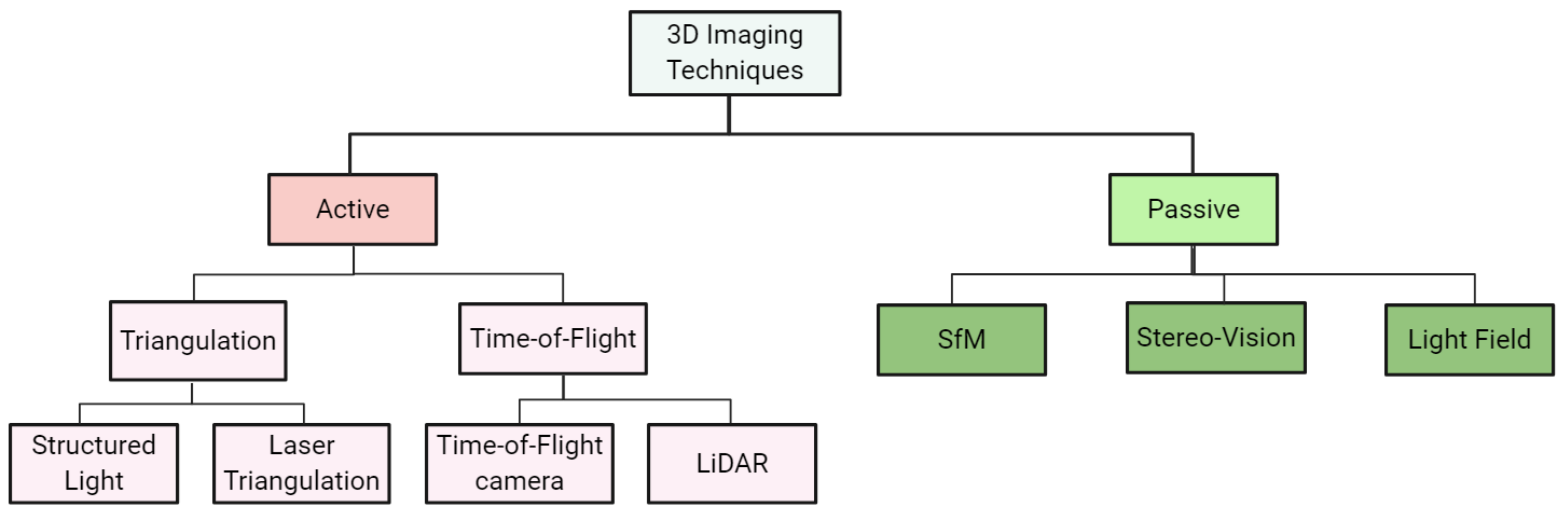
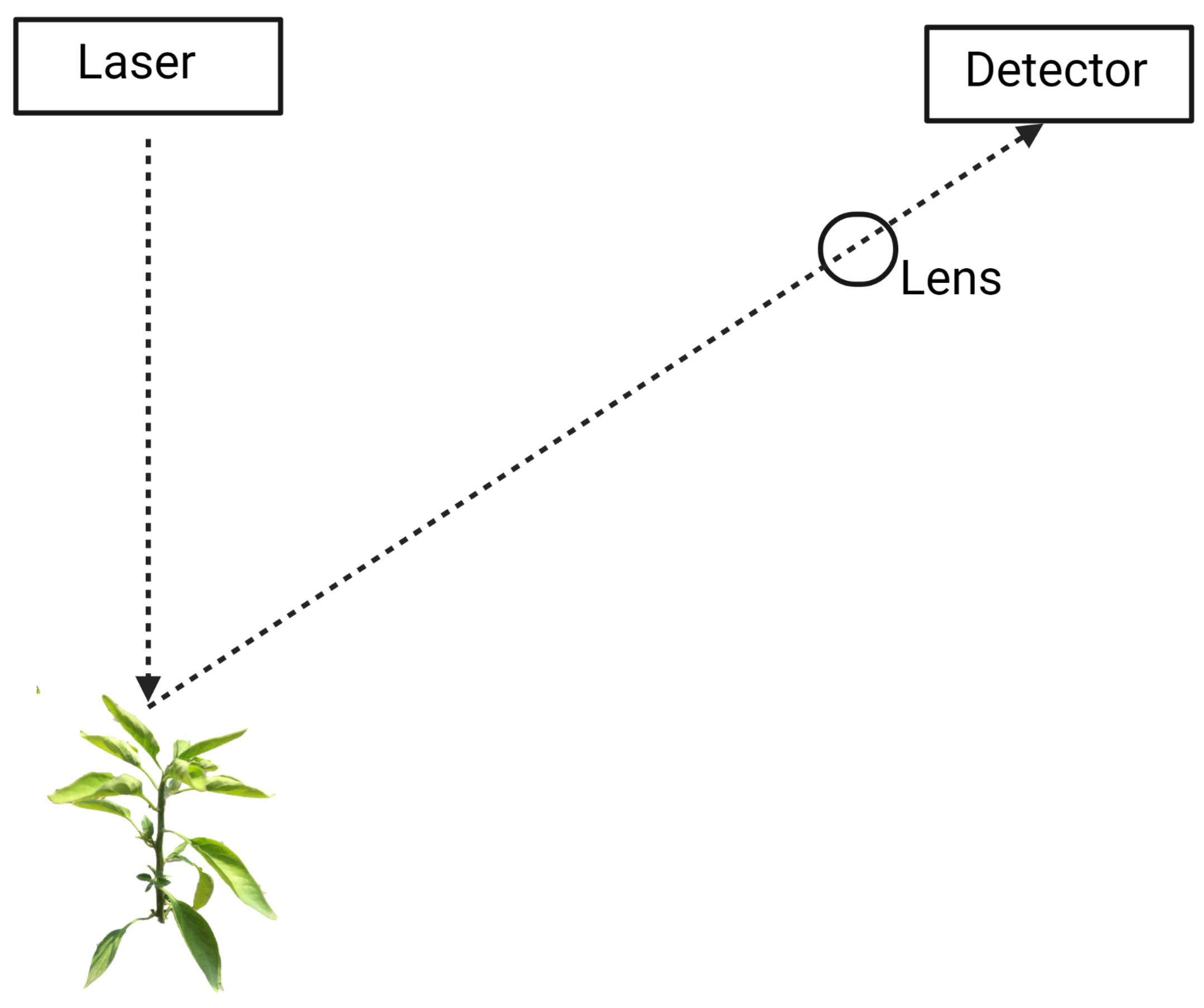
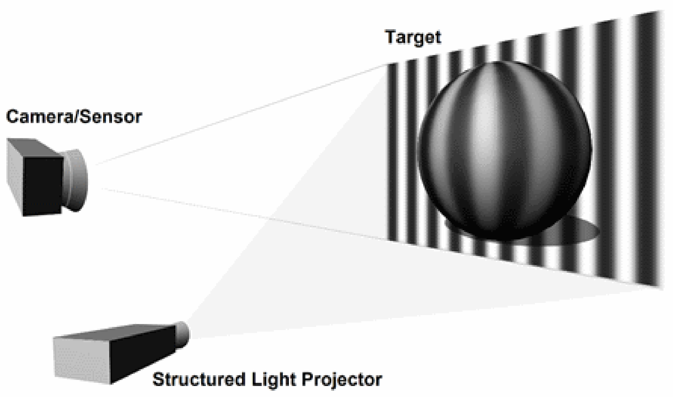
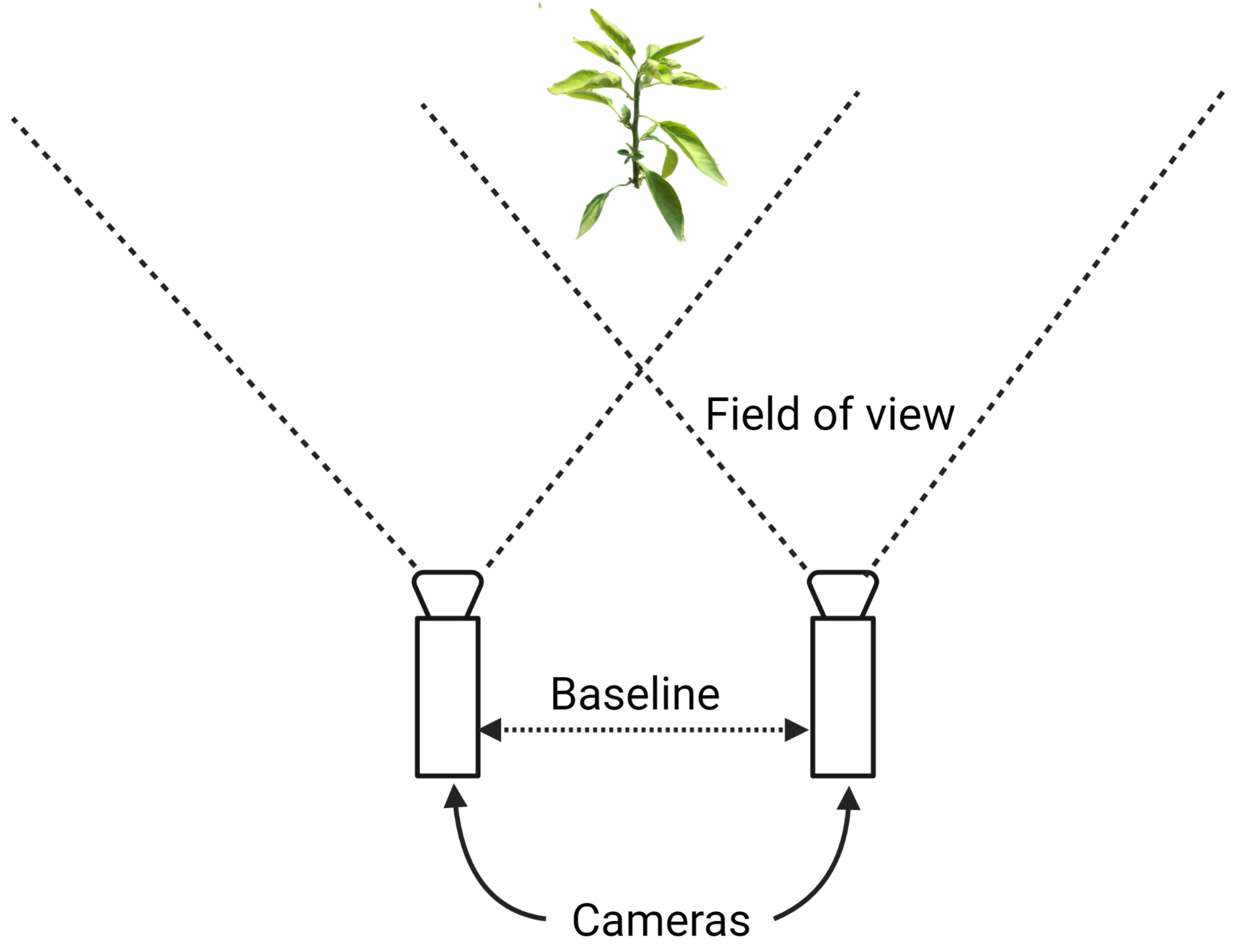
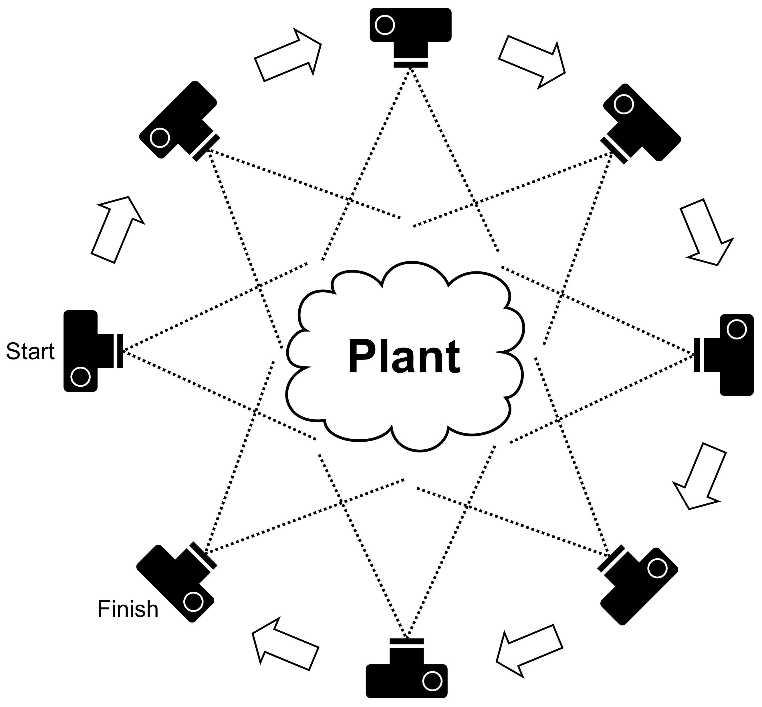
Table 1.
Comparative analysis of state-of-the-art 3D acquisition systems.
| Method | Price | Type | Output | Resolution |
|---|---|---|---|---|
| Structured Light | $$ | Active | XYZIRBG | <mm |
| Laser triangulation | $$$ | Active | XYZI | <mm |
| Structure-from-motion | $ | Passive | XYZRGB | mm |
| LiDAR | $$$ | Active | XYZ(I/RGB) | cm |
| Field cameras | $$$ | Passive | XYZRGB | mm |
| Time-of-flight | $$ | Active | XYZI | mm |
Table 2.
Comparative analysis of 3D imaging techniques.
| Technique | Type | Advantages | Disadvantages |
|---|---|---|---|
| Laser Triangulation | Active | -High precision -High speed data acquisition & 3D model generation -Do not rely on external light source | -High cost -Sensitive to sunlight |
| Structured Light | Active | -Low cost -High speed -High spatial resolution | -Small field-of-view -Poor with shiny surfaces -Limited sensing range -Sensitive to sunlight |
| Time-of-Flight | Active | -Performs well in dim/dark light conditions -High pixel resolution -Accurate depth sensors | -High cost -sensitive to sunlight |
| LiDAR | Active | -Robust against sunlight -Performs well in dim/dark light conditions -Robust against interference | -High cost -Bulky set-up -Poor in edge detection |
| Stereo Vision | Passive | -off-the-shelf cameras used -Cost-effective -Easy implementation -Provides efficient RGB stream | -Correspondence problem -Depth range depends on baseline -Sensitive to sunlight -Computationally costly |
| Structure-from-Motion | Passive | -Low cost -Excellent portability -Easy to use -Works with economical cameras | -High computation time -Poor in dim light |
Publisher’s Note: MDPI stays neutral with regard to jurisdictional claims in published maps and institutional affiliations. |
© 2021 by the authors. Licensee MDPI, Basel, Switzerland. This article is an open access article distributed under the terms and conditions of the Creative Commons Attribution (CC BY) license (https://creativecommons.org/licenses/by/4.0/).
Share and Cite
MDPI and ACS Style
Paturkar, A.; Sen Gupta, G.; Bailey, D. Making Use of 3D Models for Plant Physiognomic Analysis: A Review. Remote Sens. 2021, 13, 2232. https://0-doi-org.brum.beds.ac.uk/10.3390/rs13112232
AMA Style
Paturkar A, Sen Gupta G, Bailey D. Making Use of 3D Models for Plant Physiognomic Analysis: A Review. Remote Sensing. 2021; 13(11):2232. https://0-doi-org.brum.beds.ac.uk/10.3390/rs13112232
Chicago/Turabian StylePaturkar, Abhipray, Gourab Sen Gupta, and Donald Bailey. 2021. "Making Use of 3D Models for Plant Physiognomic Analysis: A Review" Remote Sensing 13, no. 11: 2232. https://0-doi-org.brum.beds.ac.uk/10.3390/rs13112232
Note that from the first issue of 2016, this journal uses article numbers instead of page numbers. See further details here.