
Regional Ground Movement Detection by Analysis and Modeling PSI Observations
by
 , and
, and
Bahareh Mohammadivojdan
1,* ,
,
Marco Brockmeyer
2,
Cord-Hinrich Jahn
2,
Ingo Neumann
1 and
Hamza Alkhatib
1 1
Geodetic Institute, Leibniz Universität Hannover, Nienburger Str. 1, 30167 Hannover, Germany
2
Landesamt für Geoinformation und Landesvermessung Niedersachsen (LGLN), Podbielskistraße 331, 30659 Hannover, Germany
*
Author to whom correspondence should be addressed.
Remote Sens. 2021, 13(12), 2246; https://0-doi-org.brum.beds.ac.uk/10.3390/rs13122246
Submission received: 30 April 2021
/
Revised: 28 May 2021
/
Accepted: 5 June 2021
/
Published: 8 June 2021
(This article belongs to the Special Issue 3D Modelling from Point Cloud: Algorithms and Methods)
Abstract
:Any changes to the Earth’s surface should be monitored in order to maintain and update the spatial reference system. To establish a global model of ground movements for a large area, it is important to have consistent and reliable measurements. However, in dealing with mass data, outliers may occur and robust analysis of data is indispensable. In particular, this paper will analyse Synthetic Aperture Radar (SAR) data for detecting the regional ground movements (RGM) in the area of Hanover, Germany. The relevant data sets have been provided by the Federal Institute for Geo-sciences and Natural Resources (BGR) for the period of 2014 to 2018. In this paper, we propose a data adoptive outlier detection algorithm to preprocess the observations. The algorithm is tested with different reference data sets and as a binary classifier performs with 0.99 accuracy and obtains a 0.95 -score in detecting the outliers. The RGMs that are observed as height velocities are mathematically modeled as a surface based on a hierarchical B-splines (HB-splines) method. For the approximated surface, a 95% confidence interval is estimated based on a bootstrapping approach. In the end, the user is enabled to predict RGM at any point and is provided with a measure of quality for the prediction.
1. Introduction
Monitoring the RGMs and detecting any changes to the Earth’s surface is important in updating the spatial reference system [1]. This is especially of high interest in areas that are affected by activities such as salt mining, gas, and oil extraction, as well as fossil fuel storage. In this research, we focus on the modeling RGMs. The area under study is located in the region of Lower Saxony in Germany.
Ground movement detection on a large scale depends on the measurement approach, as well as the modeling technique. One necessary step is to mathematically model the measurements as a surface, therefore allowing the user to predict the changes to the Earth’s surface at any position where measurements could be unavailable. The modeling and spatial representation of such data come with different challenges. These types of data are usually contaminated with noise and outliers and the main challenges include the irregular distribution of data and the high variability of the precision of the measurements.
From the aspect of the measurement approach, there are different methods that can be applied to track the changes through repeated point-wise measurements. Conventional surveying approaches, such as levelling, the Global Navigation Satellite System (GNSS), or total station will result in a limited number of observations. Although the resulted observations are considered precise, they have low spatial density and are usually restricted to known geodetic stations. Additionally, these approaches are typically expensive, time-consuming, and usually labor-intensive [2,3,4]. The disadvantage of sparse measurements can be mitigated by using satellite-based remote-sensing methods that can provide observations on a larger scale. The advanced methods of Interferometric Synthetic Aperture Radar (InSAR), particularly the Persistent Scatterer Interferometry (PSI), are able to detect and quantify the ground deformation in the range of millimeters per year [mm/year] in many application fields [5,6,7,8]. In the current study, PSI observations are used to model RGM specifically in the area of Hanover in Lower Saxony, Germany.
The PSI observations are prone to outliers. There are observations that might deviate from the global or local distribution of the whole data set. Hawkins [9] defines an outlier as “an observation that deviates so much from other observations as to arouse suspicions that it was generated by a different mechanism”. The PSI observations show high spatial variability due to different movement behavior of neighboring scatterers. These variations might represent only an anomaly related to individual object movements, that does not necessarily follow the global ground movement in the region. To accurately model the true RGM, detecting and removing these outliers is an important step. There are a variety of methods, which have been developed to detect outliers specifically in the field of statistics [9,10]. According to Papadimitriou et al. [11], they are mainly categorized into distance-based, density-based, clustering-based, depth-based and distribution-based methods. Distance-based methods were first introduced by Knorr et al. [12], and applied by, for example, Shen et al. [13], which defines an outlier as a point from which a certain portion of the neighbouring data has a distance more than a specific threshold. However, such a method can lead to problems when it comes to non-homogeneous distributed data [14]. Breunig et al. [14] proposed a density-based approach, which is based on the Local Outlier Factor (LOF). This factor could be derived by analyzing the data distribution density. In clustering-based approaches, those data which are not assigned to any cluster are labeled as outliers [15]. Clustering for detecting outliers have been used in different applications, which deal with point clouds, such as laser scanning data and sonar data [16,17]. Distribution-based approaches focus on a standard distribution model (e.g., Gaussian) and identify outliers as those points that deviate from this distribution [9,10]. Finally, the depth-based approaches concentrate on computational geometry, and the data are divided into different layers, wherein shallow layers are more probable to contain outliers [18,19].
In detecting anomalies for spatial data, one should consider an important characteristic of these data types, which is spatial correlation. Tobler [20] expresses this as: “Everything is related to everything else, but near things are more related than distant things”. Algorithms designed to deal with spatial data can be categorized into graphic approaches [21,22] and quantitative tests [23,24]. The methods of Scatterplot [23] and Moran Scatterplot [24] can be mentioned, which work with quantitative tests in detecting anomalies. In the direction of quantitative testing, Liu et al. [25] used a local adoptive statistical analysis to detect outliers, which was tested on SAR data. Lu et al. [26] proposed several statistical outlier detection algorithms, and similarly, Chen et al. [27] introduced a robust median algorithm to detect spatial outliers.
In this paper, a data adaptive algorithm is proposed to process the data and identify the outliers. The anomalies are detected based on the deviation of the observations to a fitted model in a hierarchical approach. The algorithm considers local behavior of the data while globally testing the deviations of the observations to the model.
The other aspect in detecting RGMs is the modeling technique, which is mainly the problem of finding the underlying function in the data set as a continuous surface that best describes the behavior of the data. This makes it possible to propagate information from the positions where information is available to new positions where no data exists. Despite a flurry of activity in this area, scattered data interpolation remains a difficult and computationally expensive problem. Mostly, the developed approaches do not allow different data distributions or remain computationally inefficient [28,29]. In modeling such data, one needs to consider the fact that it contains both deterministic and stochastic parts [30]. Deterministic approaches mainly focus on the trend in the data, for example, traditional polynomial surfaces and free-form surfaces, such as Bézier, B-splines, and non-uniform rational B-splines [31] (see Bureick et al. [32]). The stochastic methods model the stochastic part of the data based on the spatial correlation among the data sets. The Least Squares Collocation [33], Gaussian Processes [18] and Kriging [34] are examples of such stochastic approaches.
In practice, for large data sets with high variability and large spatial gaps, it is challenging to choose a suitable approach. Mohammadivojdan et al. [35] modeled such a dataset by using both ordinary Kriging and Multilevel B-splines Approximation (MBA) methods. Ordinary Kriging is a powerful stochastic method that uses variograms to model the correlation among data points; however, this approach has several drawbacks. Firstly, as a stochastic method, this method best models the stochastic part of the data; therefore, in order to have a reliable estimation, the trend in the data should be modeled separately. Additionally, this method is computationally expensive, especially for large data sets. In this study, an approach based on HB-splines was adopted to model the PSI observations. Forsey and Bartels were the first to introduce a method for HB-splines refinement to interpolate a grid of data [36,37,38]. Lee et al. [29] proposed a similar approach that is also able to approximate scattered data. The suggested MBA method generates a series of bicubic B-splines functions based on a coarse to fine control lattice hierarchy. The approximation at each level is improved by a correction term from the next level, and the sum of all the levels forms the final approximation. Compared to Ordinary Kriging, the deterministic method of MBA does not require a separate model for estimating the trend, takes less computational time, and shows robust behavior against data gaps. At the same time, the disadvantage of the MBA approach lies in model selection and choosing an optimal control lattice hierarchy [35].
It is of high importance to also model the uncertainty of the approximated RGM. Therefore, based on the modeled movement, a user should be able to predict deformation at any position and have a measure of quality for the prediction. The uncertainty in the model can be due to different reasons, namely noise and data gaps. The approximated model based on MBA in each level is derived based on least squares minimization. Therefore, based on the precision of the observations, an uncertainty measure could be derived mathematically for the approximated model. However, the final model in MBA consists of more than one level. Because each level is derived from the previous one, a highly mathematical correlation exists between different levels. This makes the error propagation and the consideration in an appropriate stochastic model a challenging process. Consequently, mathematically modeling the uncertainty for the Multilevel method is not optimal, and for large data sets the process is not computationally practical.
In order to solve this issue, a non-parametric approach based on the bootstrapping method is adopted to approximate the sampling distribution of the estimated RGM. Bootstrapping is a computer-intensive method, which can be used to obtain the sampling distribution of an estimate. It was first introduced by Efron et al. [39,40]. The method is based on intensive resampling from a limited existing sample and generating new samples. Using the information from all samples, one can derive the bootstrap sampling distribution. The standard error or confidence interval of an estimate can be derived based on the bootstrap sampling distribution. However, in terms of PSI observations and approximation surfaces, this non-parametric approach provides the uncertainty of the approximated surface. The uncertainty will mainly represent the quality of the model, reflecting the general noise and data gaps.
The rest of the paper is organized as follows: Section 2 gives an overview of the data set that is used in this paper. Section 3 provides a detailed explanation of the implemented methodologies, including the basics of the surface-based modeling method and an overview of the implemented bootstrapping approach. In Section 4, the computational results of applying the above-mentioned methodologies on the data set of interest are analysed and evaluated. The main outputs of the research, along with the strengths and limitations of the methods, are discussed in Section 5. Section 6 concludes and provides a discussion on the characteristics of the developed method, and possible opportunities are presented.
2. Data
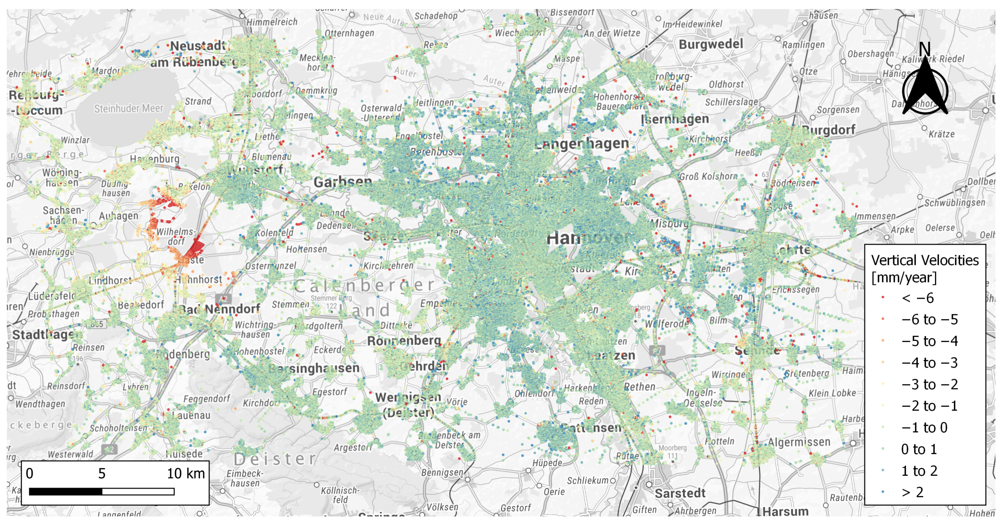
Deformation of the Earth’s surface can be caused by various geological processes or anthropogenic measures. Due to its high temporal and spatial resolution, radar interferometry provides valuable data for detecting areas influenced by ground movements. The analyzed motions in the area of Hanover are based on SAR data from the Sentinel-1 mission, which is part of the European Space Agency (ESA) Copernicus Earth observation program [41]. The identical radar satellites Sentinel-1A and Sentinel-1B were respectively launched in April 2014 and April 2016, and offer a revisiting time of 6 days on a shared orbit plane. The radar satellites operating in C-band have a spatial resolution of in Interferometric Swath mode and scan the Earth’s surface over a width of approximately 250 km. The data set for this paper provided by the BGR was generated by using PSI-WAP (Wide-Area-Product) processing [42], and contains 319226 PSI velocities. To mitigate possible large-scale errors, such as residual orbital or atmospheric errors, the PSI-WAP analysis includes independent velocities from GNSS reference stations for calibration. In the color-coded points in Figure 1, the area with ground movement caused by salt mining in the west of Hanover near Wunstorf is clearly visible. Besides this, the clustering characteristic of PSI information in urban areas and the data gaps in rural regions become apparent. The presented data material originates from an ascending satellite orbit, which covers an acquisition period from 13.10.2014 to 01.04.2018. Overall, the PSI processing contains 138 SAR images, from which the acquisition of 20.09.2016 was selected as a master scene. The derived velocities were determined in the line of sight (LOS) of the satellite and projected vertically by assuming no horizontal displacement. Horizontal displacements, especially in local ground motion areas, may lead to systematic errors of derived height changes if neglected. To separate the LOS-movement into vertical and horizontal components, a combined solution of data from ascending and descending radar satellites is necessary [43], which is out of the scope of the current paper.
The provided PSI information is corrupted by a high level of measurement errors. The measurement errors can be divided into two parts: noise and outliers. The noise in the data expresses the precision of the measured samples. By considering prior knowledge about the performance of the measurement system, this can be considered in the surface modeling process.
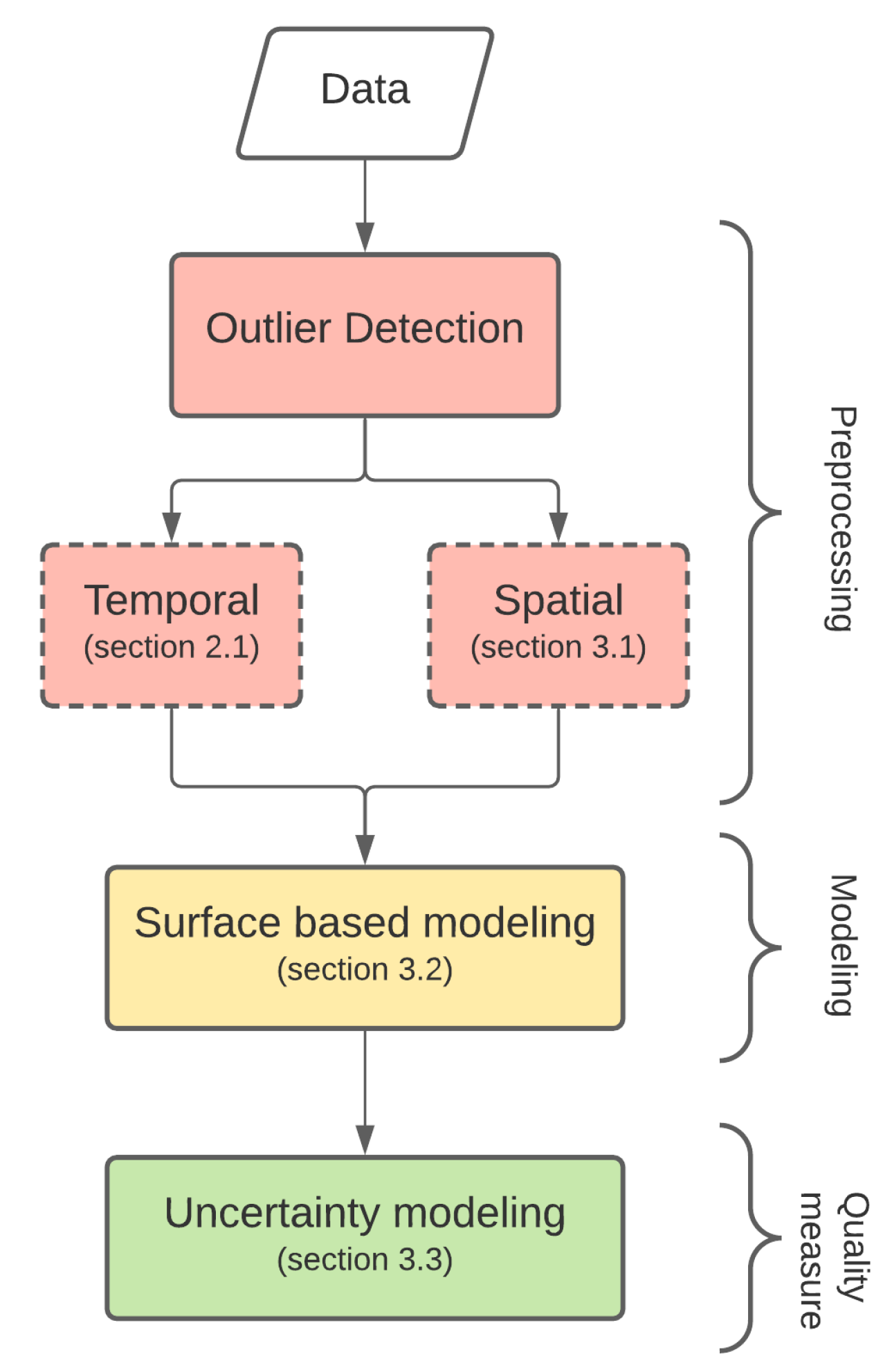
The second type of errors, outliers, are those observations that do not follow the general behavior of the neighboring points. The existing outliers can be caused by various influencing factors, such as insufficient state modeling of the unknowns in PSI processing. In addition, very local displacements (e.g., subsidence of new buildings) can also lead to anomalies, which in practice do not represent the ground motions in wider areas. Before any further processing and interpretation of the PSI velocities, the outliers have to be eliminated from the data. Those outliers which are due to very local displacements in a short period of time can usually be detected via a temporal outlier detection process [1] (Section 2.1). The rest of the spatial anomalies are to be detected in spatial outlier detection, which is the main focus in this research (Section 3.1).
2.1. Temporal Outlier Detection
The existing outliers in the time series of the scatters can be caused by local displacements in a short period of time. Hence, the time series of the height changes of the persistent scatterer were analyzed first, since they show varying quality levels. In order to identify time series with high measurement noise, a temporal outlier detection approach with subsequent elimination is adopted [1]. For this purpose, the time series of the PSI points are de-trended (by using a linear regression model) and the remaining residuals serve as a measure for the variability. If the standard deviation of the de-trended time series exceeds the defined experimental threshold of 6 mm, the scatterer is considered as an outlier and excluded from further processing.
Even after temporal filtering, the PSI velocities still show high spatial variability due to different movement behaviors of neighboring scatterers. Therefore, to remove such high-frequency outliers from the data set, a spatial outlier filtering has to be performed. Details about the adapted method is explained in Section 3.1.
3. Methodology
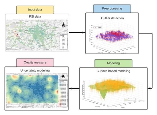
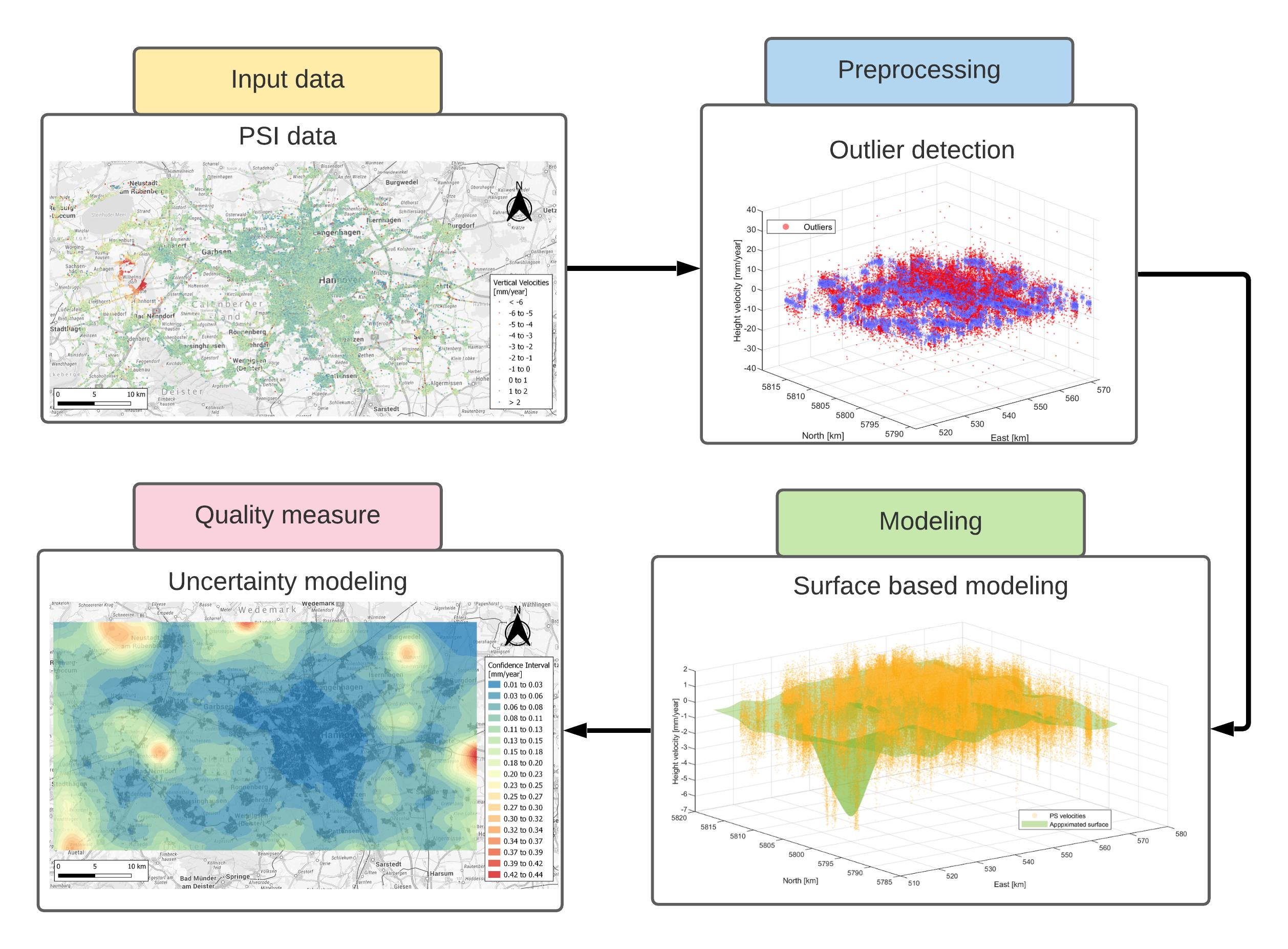
Detailed explanation of the methodologies adopted to model the PSI data are presented in the following section. Figure 2 presents a flowchart of the main steps and framework of the whole process.
3.1. Spatial Outlier Detection: Data Adaptive Outlier Detection
Some observations that might deviate from the global or local distribution of the whole data set: As described in Section 2, the PSI velocities show high spatial variability due to different movement behaviors of the neighboring scatterers. This behavior might represent individual object movements, which does not necessarily represent the global ground movement in the region of interest. These anomalies should be detected and eliminated before modeling the RGM. A data-adoptive algorithm is proposed to process the data and identify the outliers. The outliers will be identified based on their deviation or distance to a fitted model. The model is based on least squares minimization, which estimates a HB-splines surface to approximate the data. The chosen method is based on MBA that is described with details in Section 3.2.
The aim is to assess the distance of the observations to the approximated model. The observations with the highest deviation are more suspected to be outliers. However, two issues should be considered: firstly, if the model is not able to detect the local behavior of the data, or in other words, the model has some smoothing effect, some correct data may be misclassified as outliers. More precisely, some large deviations may be detected as a result due to the low complexity of the model. The second issue is the masking effect of the outliers, meaning that if there are extremely large outliers in a neighborhood, it may affect the model estimation. Consequently, the estimated model will be shifted toward the outliers and some correct observations might be misclassified as outliers, or some genuine outliers may not even be detected.
In order to mitigate these challenges, the process of detecting outliers is broken down into a few iterations. At every iteration, we model the data. Then, the deviations of the data to the model are calculated. The estimation of the model is based on least squares. Therefore, the assumption is that the residuals, or the deviations to the fitted model, are normally distributed. Considering the distribution of the residuals, those data points with residuals larger than a threshold are identified as outliers. The threshold for distinguishing between outliers and clean data is defined as a multiplication of the residuals standard deviation () by a factor (T). In this paper, based on a sensitivity analysis, T is chosen to be 3, and the process of choosing this parameter will be explained in more detail in the following. Then, the detected outliers are eliminated, and the remaining data will be processed in the next iterations. The iterations will be terminated when the distribution of the residuals is close to the expected noise of the data set (Algorithm 1). The reason for this criterion is that the goal is detecting outliers, avoiding over-fitting the data, and modeling the noise. An overview of the adopted symbols in the Algorithm is presented in Table A1 (Appendix A).
| Algorithm 1: Outlier detection algorithm. |
 |
In the first iteration, a coarse global model is used to approximate the observations . It will result in a rough approximation of the data. However, for choosing the initial model, a minimum complexity should be considered. A very simple model would result in assigning normal observations to outliers , which could be avoided by taking into consideration prior knowledge about data behavior. In each iteration, the complexity of the model increases. Increasing the complexity of the models from one iteration to the next will help to gradually take the smoothing effect of the approximation into account.
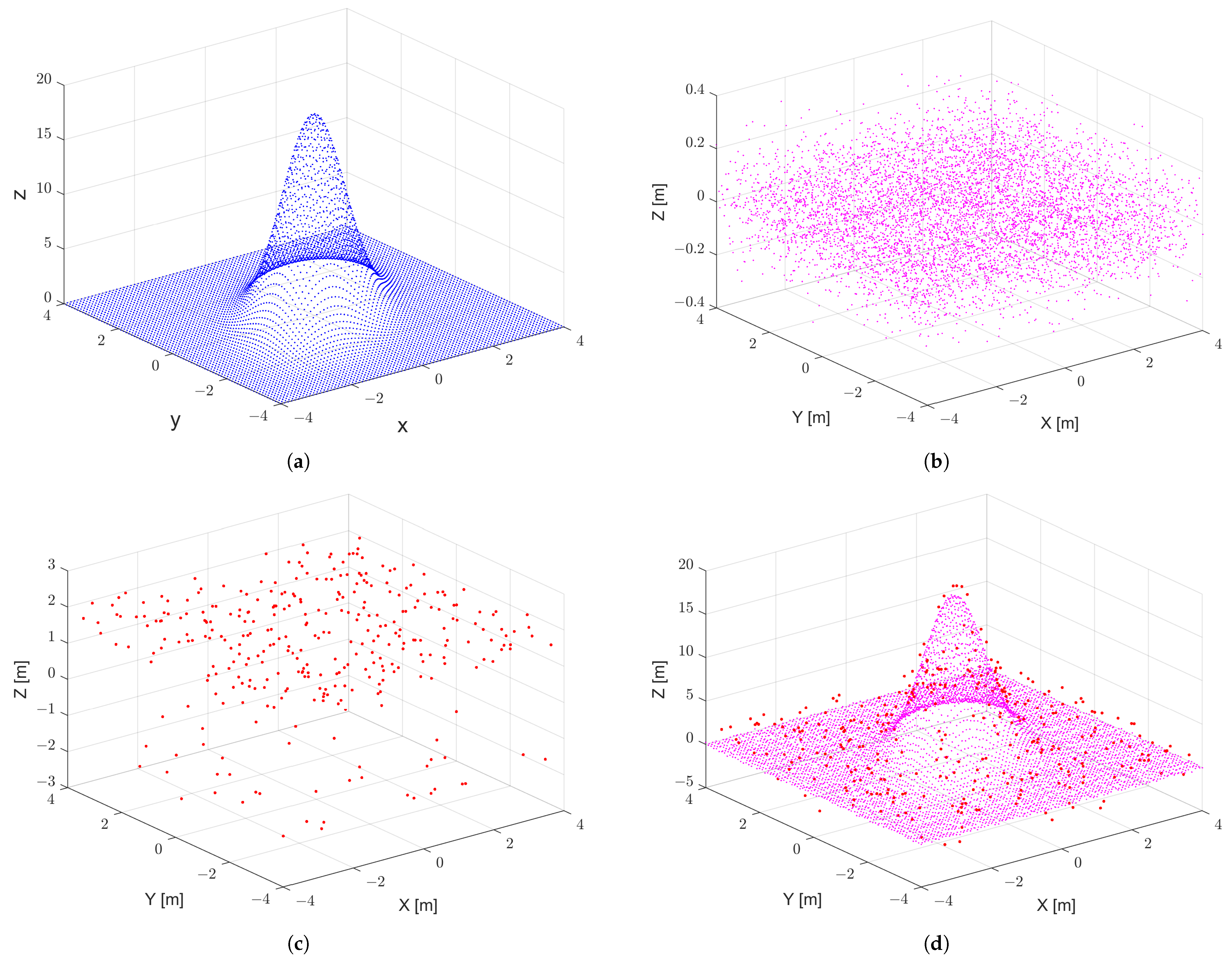
In order to assess the accuracy of the proposed method, the outputs are compared with reference data in which the genuine outliers are already known. For this purpose, a reference data set is simulated. The simulated data are a point cloud with three components. Only the z-component is stochastic, while the x- and y-components are assumed to be deterministic. The simulated data set consists of three parts: trend, noise and outliers. The noise is generated from a Gaussian distribution with zero mean and a standard deviation of m. In addition, the outliers are randomly generated from a Chi-square distribution. The range of the Chi-square distribution lies in the tails of a Gaussian distribution with zero mean and standard deviation of m. The simulated data represent a scenario in which the measured data contain noise, as well as large outliers. A realization of the simulated reference data is illustrated with different parts in Figure 3. To ensure the functionality and performance of the algorithm, it is tested in a Monte-Carlo (MC) simulation. In each MC run, a new set of noise and outliers are generated.
The algorithm can be seen as a binary classifier that categorizes the points into inliers and outliers. The two outcomes of the classifier can be positive (outlier) and negative (inlier). The results can be expressed in a two-by-two confusion matrix (Table 1). True Negative (TN) and True Positive (TP) present the outcomes in which an actual inlier and an actual outlier are correctly predicted, respectively. False Negative (FN) and False Positive (FP) represent the cases where an instance is assigned to the wrong class. To assess the performance of the algorithm, four measures of precision, recall, the -score, and accuracy are used, which are calculated based on the following formulas (Equations (1)–(4)).
The results of the algorithm for different percentages of outliers and noise levels are presented in Table 2. Each measure is the median of all calculated values for 1000 MC runs. The whole simulated data set consists of 6561 points, and in the three scenarios, the generated outliers are 5%, 10% and 15% of the data. The level of noise also varies for three cases, and it shows the standard deviation of the Gaussian distribution from which the noise is generated. For noise with m, by considering 5% outliers, precision is more than 90%. This means that the ratio of the correctly classified outliers is high. Recall or sensitivity shows the ratio of detected outliers to the actual outliers. A recall of 1 means that all the outliers are detected. However, some inliers are also classified as outliers (here the median is 34). Such wrong classifications are best expressed by a -score, which is the harmonic mean of precision and recall. For 10% of outliers, the algorithm still performs well; however, this is no longer the case for 15% of outliers. Although with high percentages of outliers the precision is still good, the sensitivity of the algorithm is decreased. Such an effect can be improved by optimizing the selected criteria for eliminating the outliers in each step, which is not the focus of the current paper. Furthermore, by increasing the noise level, the sensitivity is affected. This is more critical when the noise level is close to the outliers’ distribution; meaning with a high level of noise, it is difficult to distinguish between the noise and outliers.
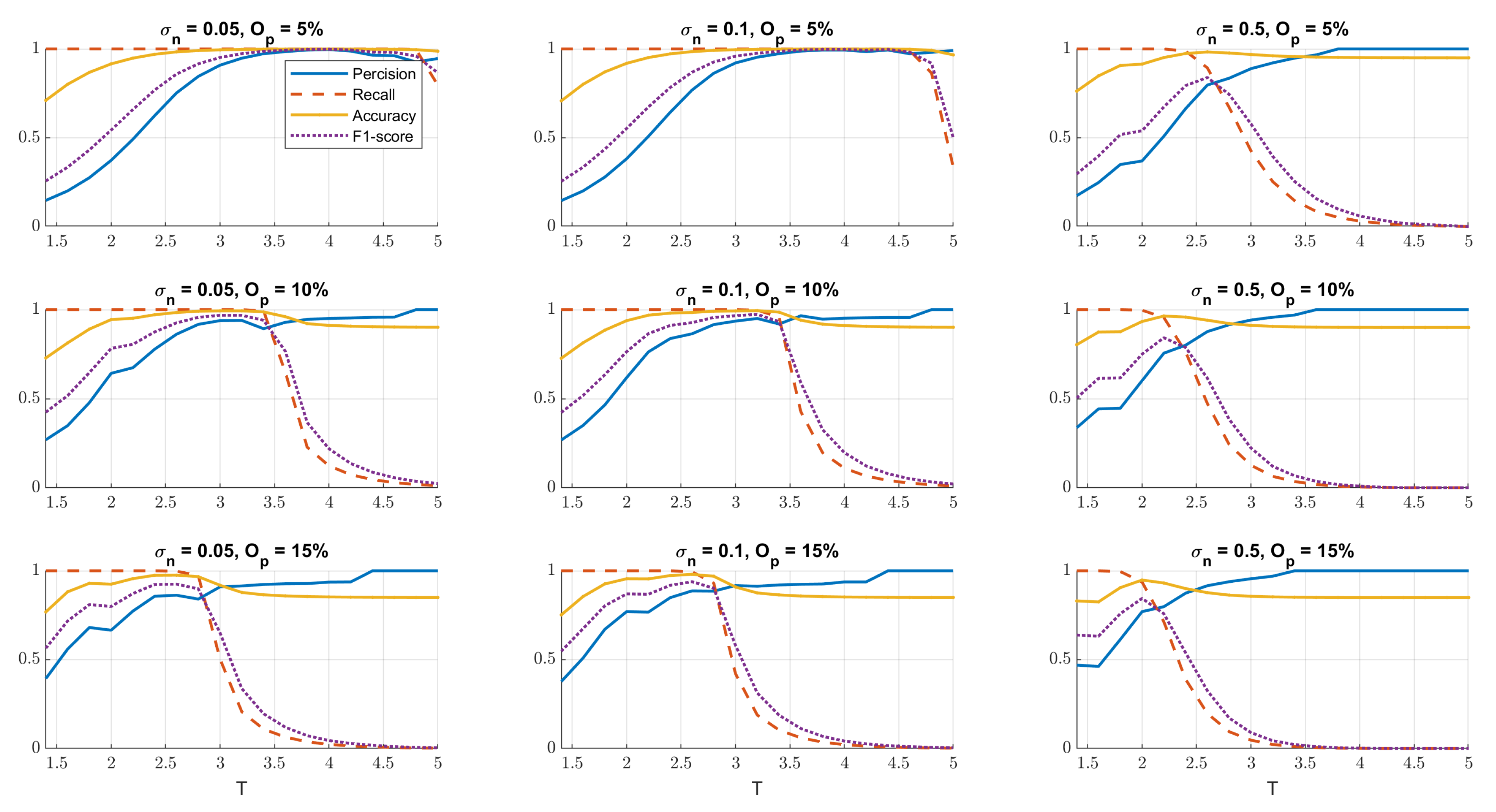
To choose a suitable threshold for detecting outliers in each iteration of the outlier detection algorithm, we performed a sensitivity analysis. The value of the threshold is increased incrementally by changing the multiplayer T between 1.5 and 5. The performance of the algorithm with respect to different threshold values in the range of is illustrated in Figure 4, by means of the four mentioned parameters: precision, recall, accuracy and -score. In Figure 4, the results related to the three mentioned scenarios and the different outlier percentages are presented. The best performance of the algorithm occurs when factor T is in the range of , for the first two scenarios where is 0.05 and 0.1. The optimal value of the factor T is also sensitive to the outlier percentage. For lower percentages, higher T values would suffice, and where more outliers are included in the data, smaller values perform better. As explained previously, the last scenario () does not perform well even with different T values. The reason is the high range of noise, which makes it difficult for the algorithm to distinguish between noise and outliers. In this paper, for the factor T, the value of 3 is chosen and used.
3.2. Multilevel B-Spline Approximation (MBA)
According to Section 2, the PSI observations of interest here represent a large area. The 3D point cloud of PSI observations can be described as scattered data, since only vertical velocities are considered. The data set contains a high level of noise, and due to the clustering characteristics of PSI observations, especially in urban areas, the data set is irregularly distributed. This varying density of the point cloud causes large areas with very low density or no observation (data gap). The scattered data set does not provide information on the connectivity between the points, and considering the mentioned characteristics of the data, the global behavior is not visible. Therefore, it is important to understand the underlying pattern in the data. By finding a suitable mathematical model that describes the underlying function, the noise in the data can be eliminated and a prediction surface for the data gaps derived, and as a result, the global behavior of the data set will be uncovered.
In conversion from discrete points to a continuous surface, a deterministic technique based on free-from surfaces is used [44]. The MBA method is an approximation method based on hierarchical tensor product B-spline surfaces. This method was first developed in the 1990s for specific image-processing applications, such as image morphing [45,46]. Lee et al. [29] introduced a modified version of this approach that can handle scattered data. The B-spline surface is defined by a control lattice that contains control points. If we assume is overlaid on the domain , any control point on the lattice overlaps with the integer values of . The B-splines surface f is defined as a linear combination of uniform bicubic basis functions , and control points of a control lattice , wherein .
The uniform cubic basis functions for are defined as follows,
Similarly, the basis functions are calculated. Let be the proximity data points of each control point. The proximity data are those points that lie in the neighborhood of a control point . For each point in the proximity data set of a control point, one solution can be derived . The unique solution for a control point is derived from minimizing the error term for all points, wherein , , , , . The minimization is solved by means of a Least Squares method, and the final solution is as follows:
wherein . It should be noted that when the proximity data set is empty, it implies that does not influence the B-splines surface function (Equation (5)) and therefore, any value can be assigned to the aforementioned control point. In this case, here a value of zero is assigned to .
In their proposed algorithm for MBA approximation, Lee et al. [29] used a hierarchy of control lattices to generate a sequence of . The sum of all B-splines surfaces in the hierarchy approximates the final desired surface. The approximation starts with a rough estimation, and the resolution of the control lattices increases in each step. For approximation, at the first step, a hierarchy of control lattices , , …, are defined, where the first control lattice is , and the lowest number of control points is the coarsest one. On the other hand, the last control lattice, is the finest control-point lattice, which contains the highest resolution of control points. The approximation process starts with the coarsest control-point lattice . Afterwards, by using the deviation of the estimated function to the original observations based on , the control lattice of the next level is estimated. Such a process should continue until the last control lattice is estimated. In general, at each level k, for estimating the control lattices, the function is calculated based on .
The final approximation function is defined as the sum of functions in the hierarchy as follows,
As mentioned, the PSI data is a large data set that also contains large data gaps. These gaps in the data not only introduce uncertainty to the modeled surface, but also create numerical instability. The characteristics of MBA make it suitable to model the PSI data. The proposed MBA algorithm by Lee et al. [29] is computationally efficient and the method can easily handle large data sets. The model is numerically stable because in the estimation of the unknowns, no inversion is required, and in combination with the regularization option in the function, the method is powerful in dealing with data gaps.
3.3. Bootstrapping
The final approximated model is influenced by different elements, such as measurement error, data gaps and the complexity of the chosen model. Therefore, it is important for a user to have a measure of quality for the approximated surface. Based on the explained method in Section 3.2, the approximated model based on MBA in each level is derived with least squares minimization. Therefore, mathematically, a measure of uncertainty for the model can be derived based on the precision of the observations. However, the final model in MBA consists of more than one level. The levels are approximated sequentially based on the previous ones. This creates a highly mathematical correlation between all layers. This makes error propagation a challenging process. Doing so makes the process computationally expensive and impractical in cases where there are large data sets. To overcome this problem, we have adopted a non-parametric method called “bootstrapping”.
Bootstrap is a computationally intensive method, which was first formulated by Efron et al. (e.g., [47,48]) to simulate a statistic distribution. This method provides the possibility of inference from an existing sample with a limited size and no information about the data distribution. The idea is to intensively resample from the existing samples to generate new ones. The new samples are called “bootstrap samples”. Afterwards, information from the empirical distribution of each bootstrap sample could be extracted. Combining the information from all bootstrap samples will provide the possibility to infer the distribution of the desired statistics related to the main population. Here, the goal is to get information on the distribution of a predicted point through bootstrapping. The variations of the predicted point, or in other words, of the model at a given location, need to be investigated by applying different bootstrap samples. The variations will result in a histogram showing the distribution of the predicted point. From this distribution, we can describe the standard deviation and confidence interval of the predicted surface at a specific position.
In the first step of calculating the standard deviation of the approximated surface based on this method, the bootstrap samples () should be formed. A bootstrap sample is generated from the original observations (). Any point in the bootstrap sample is drawn randomly and with equal probability from the original sample. In practice, the size of the original sample may be large, and it might not be possible to enumerate all possible bootstrap samples. Instead, a large number (B) of bootstrap samples are independently drawn from the original sample.
In the scope of this paper, the goal is to get the standard deviation of the approximated surface based on the original PSI observations at a desired position. Based on each bootstrap sample, a surface is approximated, which leads to available predictions at the desired position from all bootstrap samples at the end (). This will represent the possible variations of the prediction and its distribution. Based on the distribution, the related bootstrap standard deviation () can be calculated as follows,
wherein represents the mean of the bootstrap predictions at the desired position.
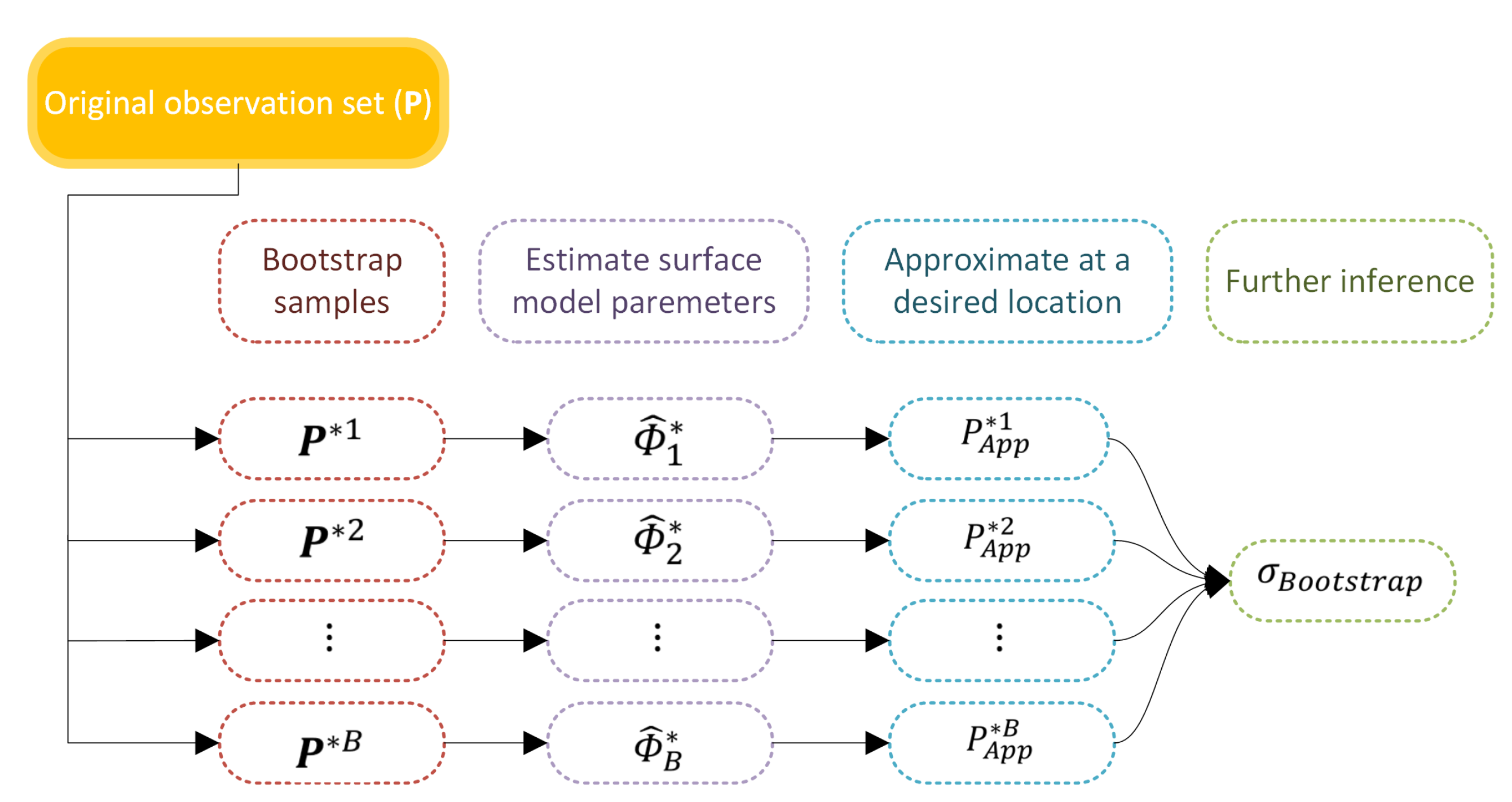
A confidence interval (CI) of the predicted surface can also be obtained non-parametrically. For a specific significance level of , a CI can be computed based on the sorted predicted values from the smallest to the largest [49,50]. The lower and upper bound of the CI are the th and th values, respectively. In the case of non-integer numbers, the nearest integer value is selected. Figure 5 illustrates the explained bootstrapping algorithm which is implemented (see Algorithm 2). An overview of the adopted symbols in the Algorithm is presented in Table A1.
| Algorithm 2: Bootstrap Algorithm. |
 |
As a result, point-wise standard errors can be derived. We can get information on possible variability of the prediction. The bootstrapping algorithm does not require theoretical calculations and provides information even for complicated problems. It should be noted that the dispersion of the distribution related to a predicted point is dependent on the observations, as well as the complexity of the modeled surface. Additionally, in areas with less observations, the distribution will be stretched. Moreover, if the chosen model is over-fitting the data, it leads to an increase in the uncertainty range.
4. Results
This section entails the results of applying the explained methods from Section 3 on the data set of interest (Section 2). In the first step, the data are pre-processed (Section 4.1) by using the proposed outlier detection algorithm (Section 3.1). After eliminating the outliers, in Section 4.2, the observations are modeled as a continuous surface according to the explained surface approximation technique in Section 3.2. At the end in Section 4.3, 95% CIs are derived for the approximated surface based on the bootstrapping method (Section 3.3).
4.1. Pre-Processing of Data
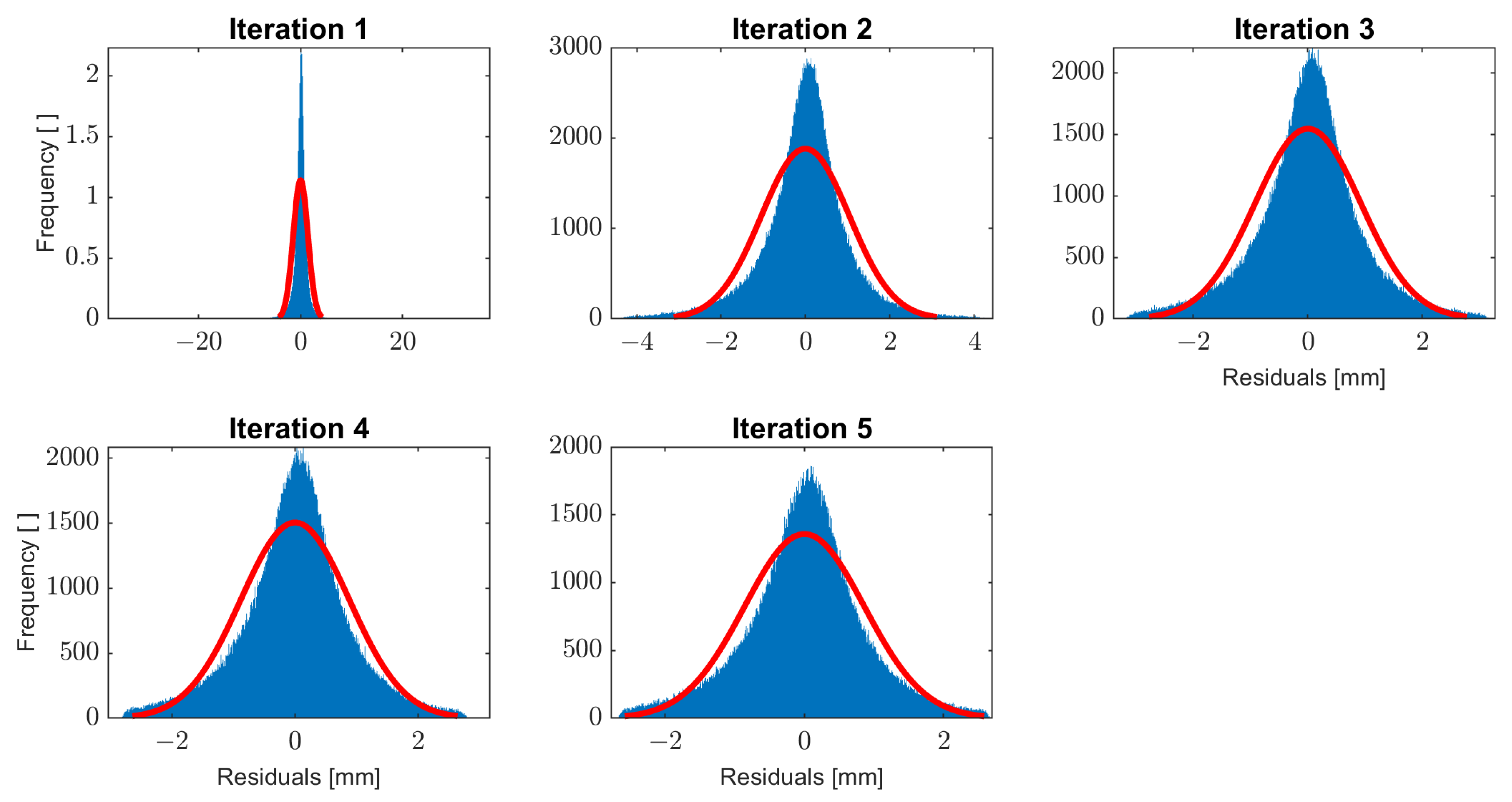
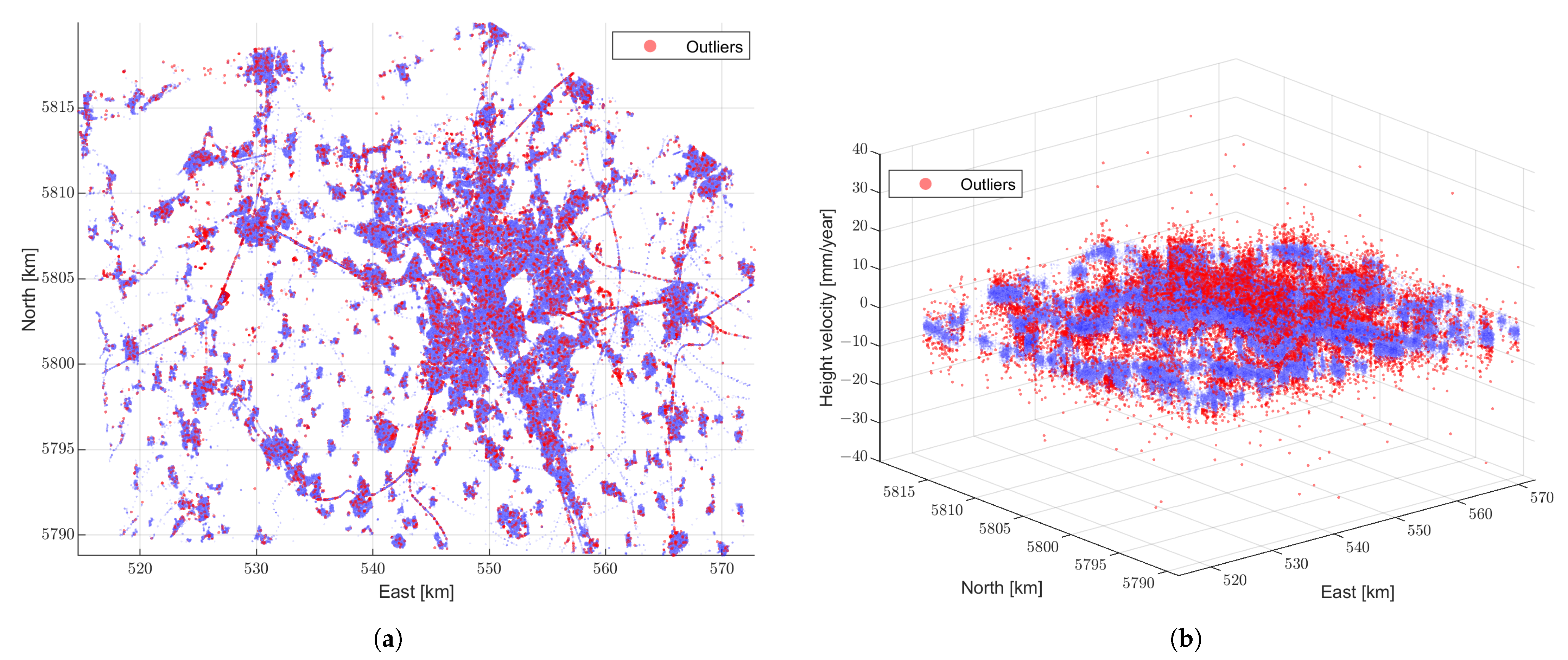
The real data, introduced in Section 2, are first processed for spatial outliers based on Algorithm 1. The data set contains 301,386 observations. After running the algorithm, 15,201 outliers from 301,386 data points are detected. The process takes five iterations. The initial model starts with two levels and in each iteration, one layer is added to the control lattice hierarchy in such a way that the next layer has five more control points in each direction. The noise level in the data are not known, and therefore based on the dispersion of the data around zero, a suitable noise level is chosen as a stop criterion for the algorithm. Since the data are not normally distributed and also contain outliers, two-thirds of the standard deviation is used. In Figure 6, the histogram of residuals from different iterations is illustrated. The improvement in the shape of the histogram of the residuals from one iteration to the other could be seen. The final histogram is still not exactly normally distributed, but it is symmetric and is centered around zero. Figure 7 illustrates the detected outliers and shows reduction of noise in the observations.
The genuine outliers are not known in this case, and therefore, to evaluate the accuracy of the proposed algorithm, we try a comparison to a similar study. This data set has been processed by Brockmeyer et al. [1]. They used a local neighborhood analysis to identify the outliers. By comparing the individual PSI velocities with the associated neighborhood functions, spatial variations are detected as outliers with a given probability of error [1]. As a result of the conducted outlier detection, 15,609 PSI velocities were detected as outliers. This method has two disadvantages: firstly, it only compares the points locally, and secondly, it requires a high computation time. Because each point is tested individually, it therefore becomes even more challenging in large data sets. The output of our algorithm is compared with results of [1], which are shown in Table 3. The results show high compatibility of the estimations from both algorithms. The precision and accuracy is high in comparison to recall, which means that the algorithm has classified some of the outliers from [1] as inliers.
4.2. Approximation of RGM
The next step after pre-processing the data and eliminating the outliers is to mathematically model the height velocities followed by approximating a continuous surface, which represents the RGM in the area of Hanover. The RGM is approximated based on the MBA method (Section 3.2). Based on the nature of the data set and prior information of the general ground behavior of the region, a control lattice hierarchy of three levels is used. Figure 8a illustrates the approximated surface along with the observed height velocities. In more detail, the approximated RGM is presented in Figure 8b as a color-coded map. Aside from local movements (in the range of [mm/year]) to the Earth’s surface, a large movement up to –6 [mm/year] is observed in the left side (area of Wunstorf).
4.3. Confidence Interval
Even after pre-processing and eliminating the outliers, the remaining PSI velocities contain high levels of noise. Additionally, spatial distribution of the velocities is non-homogeneous, and there are large areas with sparse observations (Figure 7a). This introduces a high level of uncertainty to the approximated RGM model (Section 4.2). To derive an uncertainty measure that best describes these effects on the approximated model, the bootstrapping method is implemented in accordance with Section 3.3.
As described in Section 3.3, at first, the bootstrap samples are generated. The observation sample after eliminating the outliers still consists of 286,185 points; therefore, practically all the 286,185 possible samples cannot be formed. Instead, a large number of bootstrap samples (B = 1000) with equal probability is drawn from the observations. Afterwards, for each bootstrap sample, the RGM is modeled.
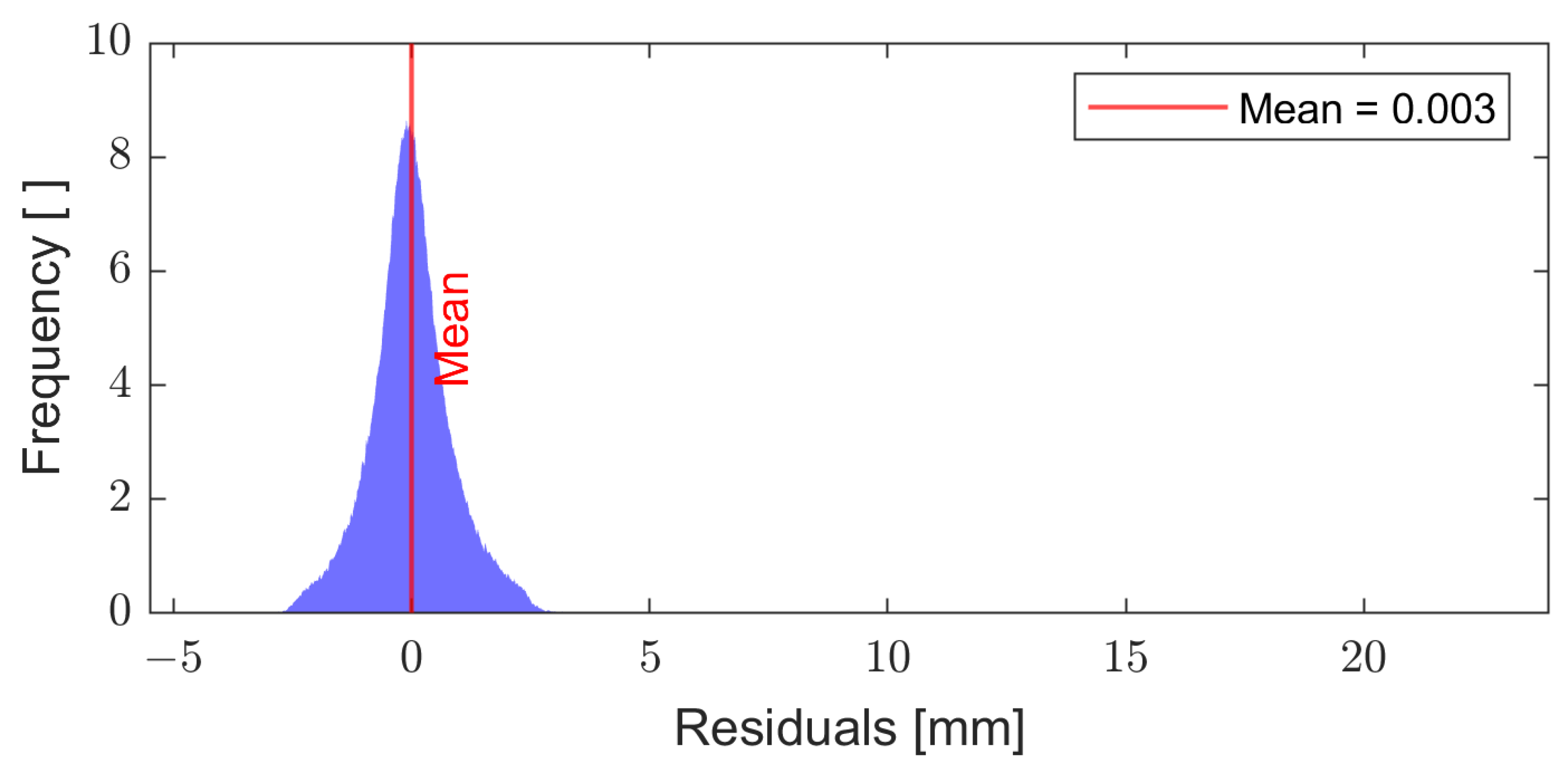
To assess the quality of the approximated model, the difference between the PSI velocity and the predicted value can be used as an error measure. These differences or residuals are calculated for all the points in the observation set, over all approximated models related to the bootstrap samples (). The results for all residuals (1000 × 286,185) are illustrated in Figure 9. The histogram shows that the residuals are symmetrically distributed. However, there is a number of large deviations (around 20 [mm/year]) related to a specific area in the observations where sharp local deformations have been observed, which was not detected by the adopted model.
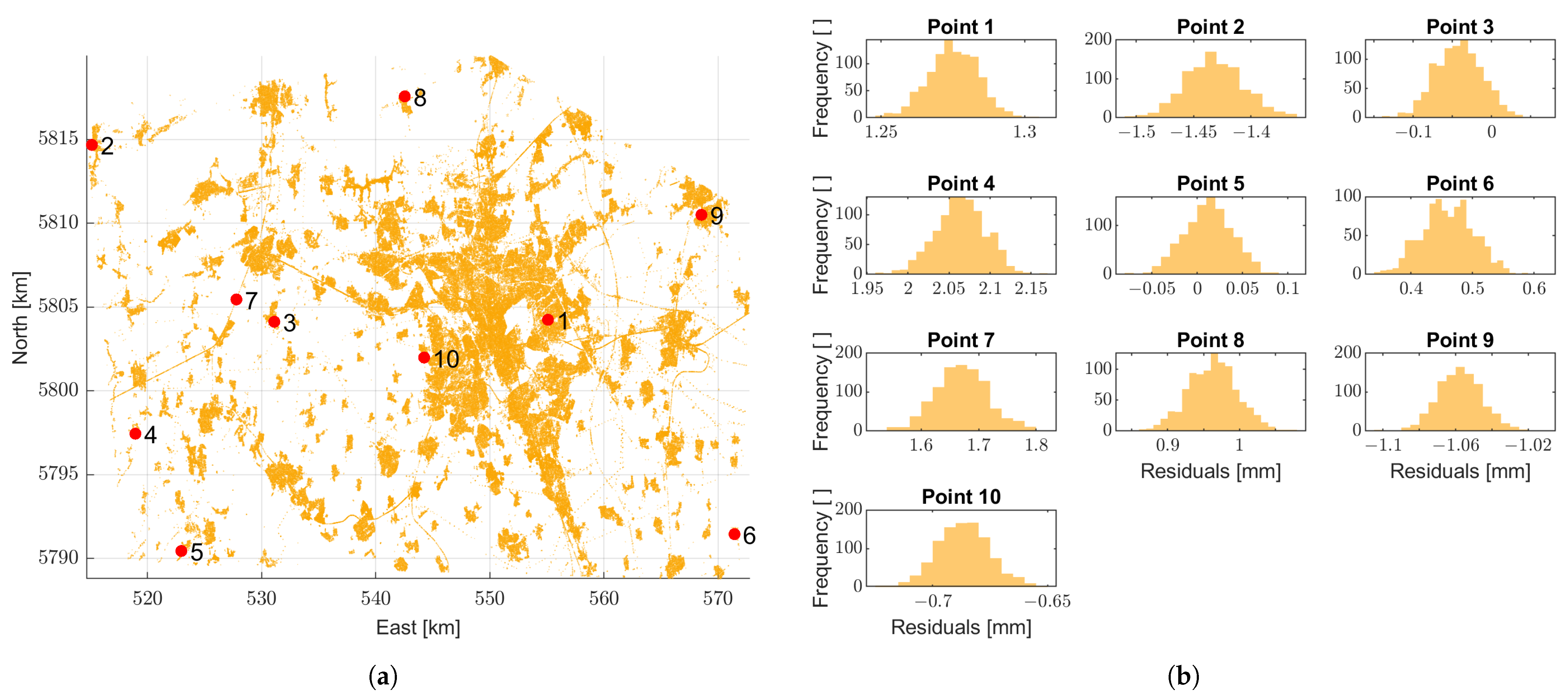
In more detail, the variations of predictions () through all bootstrapping iterations for 10 arbitrary points are assessed. The 2D view of the location of these 10 chosen points along with the histograms are shown in Figure 10. Histograms show less variations in areas with more observations. The spread of the histograms is also affected by the spatial distribution of neighboring points. This effect can be seen, for example, in the difference in histogram for point 1 and point 6. Point 1 is located in an area with many observations in the neighborhood. On the contrary, point 6 is in a sparse area. Such a neighbourhood effect is directly reflected in the spread of the derived histograms and the corresponding bootstrap standard deviations ( for point 1 and 6 is 0.008 and 0.04 [mm/year], respectively). The histogram of observations for the points individually is not symmetrically distributed in all cases; however, the histogram of all the points for the whole region represents a symmetric distribution (see Figure 9).
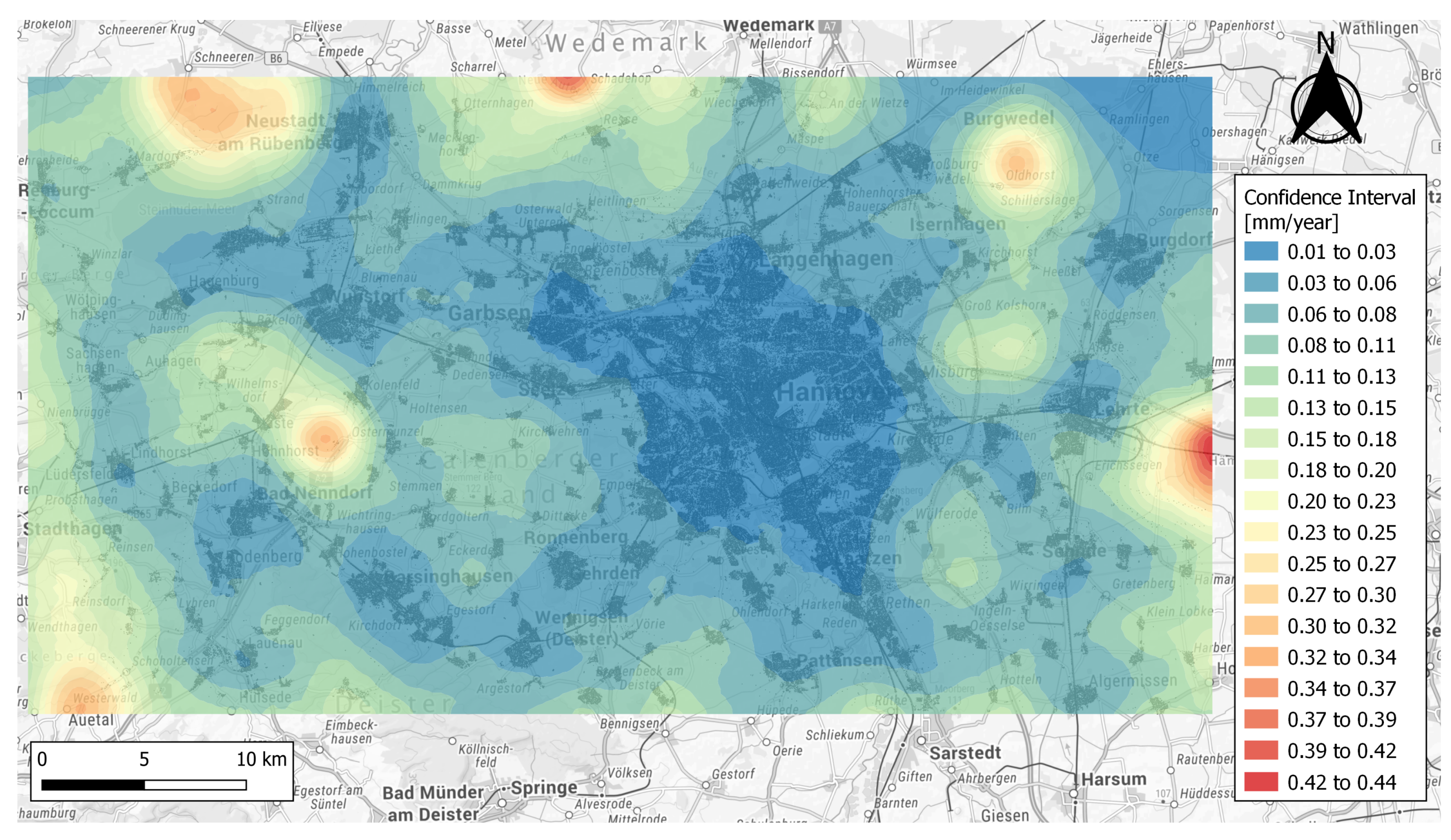
Based on the performed bootstrapping process, a 95% confidence region can be obtained for the whole area. The CI is calculated from the quantiles of the bootstrap predictions. In Figure 11, the range of the CIs is represented as a color-coded surface. The range is derived based on the difference between the lower and upper bounds of the percentile interval. For the whole area, the lengths of the CIs are between 0.01–0.4 [mm/year]. The minimum and maximum bootstrap standard deviations () for the whole region is 0.003 [mm/year] and 0.13 [mm/year], respectively.
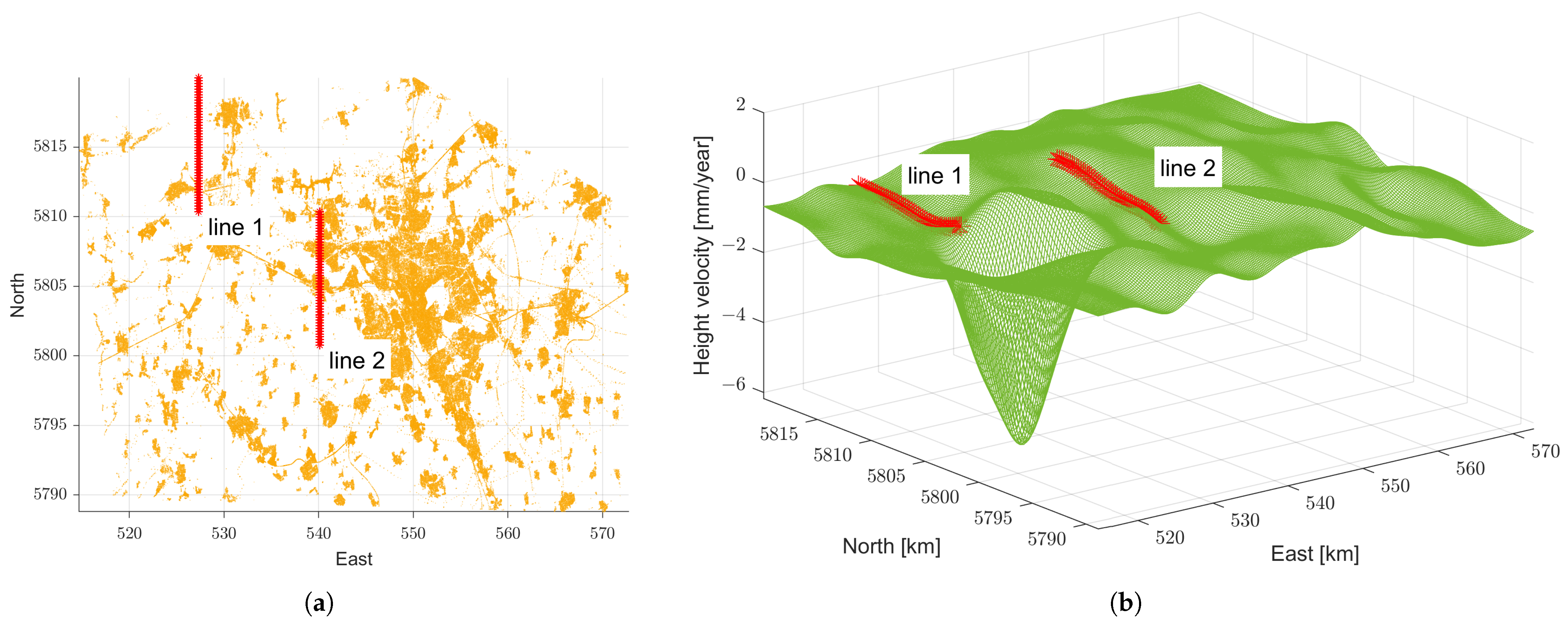
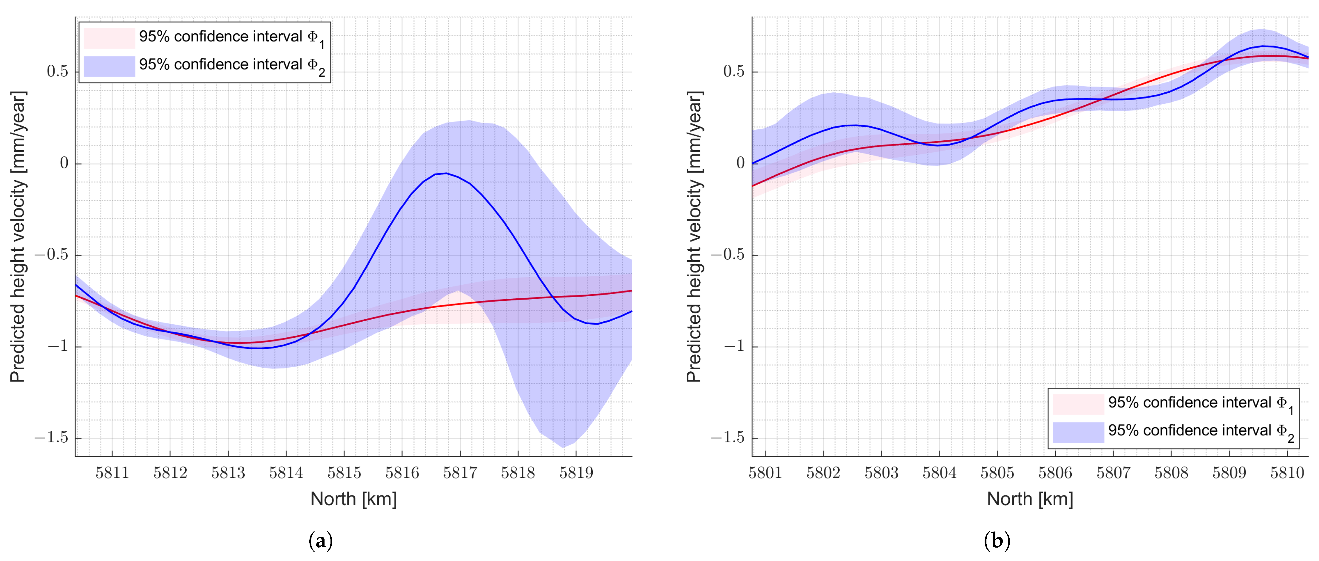
The range of the CI of the approximation highly depends on spatial distribution of the points. In the areas where less observations are available, there will respectively be less observations in the bootstrapping sample, which directly affects the model. As a result, the range of the CI in such regions increases automatically. In a closer look, such an effect can be seen for example in two selected lines that are specified in Figure 12. In Figure 12a, the position of the observations and the lines of interest are presented. Line 1 is situated in the edge, and less observations are available in its neighbouring area. On the other hand, line 2, which is closer to the middle region, is in an area with more observations. It is expected that in areas with less observations, the approximated model is more uncertain and shows higher variability in the distribution of prediction from bootstrap samples. This can be observed in Figure 13. The CI of line 1 (see Figure 13a) shows that the approximated model towards the edge of the area is highly uncertain, as expected. In contrast, the interval is relatively small for line 2. The confidence bands describe the uncertainty of the approximated model in Section 4.2, where all observations are used to model RGM. In Figure 13, the continuous line represents the mentioned approximated model, and the dashed line is the median of the approximations based on the bootstrap samples. The median lies mostly over the approximated model.
As explained, the CIs (see Figure 11 and Figure 13) describe the uncertainty of the approximated model by considering all the observations for the chosen control lattice hierarchy in Section 4.2. However, the range of the interval depends also on the complexity of the chosen model. This effect can be seen in Figure 14. The estimated CI for the two lines are calculated for two different models with the following control lattice hierarchy for the two models: and .
5. Discussion
The proposed spatial outlier detection algorithm shows compatible results to the study by Brockmeyer et al. [1]. Since the ground truth behind the distribution of the outliers in the real data is not known, it is not possible to evaluate these results more comprehensively. The algorithm not only considers both local and global behavior of the data, but the iterative process of the algorithm also helps to detect the anomalies more precisely. By fitting a surface to the data in each iteration, the nature of the data which represents a surface is taken into account. This makes the approach especially suitable for these kinds of applications. The performance of the algorithm will be improved by having some prior knowledge of the data set. For example, information regarding the minimum noise level and rough expected RGM would help to decide on the complexity of the models for the first and last iterations.
The MBA approach showed computational efficiency and numerical stability in dealing with the real data set. Therefore, it is possible to choose a very complex model with a high number of control points and many levels; however, the approximation of the data based on the MBA approach is very sensitive to complexity of the chosen model. To avoid over- or under-fitting the data, an appropriate control lattice hierarchy could be selected based on the type of dataset and the prior information about the general ground behavior of the region.
The calculated confidence bounds describe the quality of the model very well. The effect of data gaps and noise is directly reflected on the range of the CIs. In this research, the CIs are determined based on the quantiles; however, an improved interval or the ’bias-corrected-’ could also be calculated [47].
The range of the CIs is also influenced by the complexity of the model. Increasing the complexity increases the uncertainty range of the approximation. This is particularly important when there is a risk of over- or under-fitting the data or, in other words, the model selection problem. The information from the CIs and standard deviations of the bootstraps can be helpful in finding the most appropriate model for a given data set. This could lead to a solution to solve the model selection problem in similar situations. In the present work, the initial model selected is based on the prior information of the global movement in the region. The model selection concept is not the focus of the current paper.
In practice, the output of this process will help to detect areas affected by movement. By considering the additional information on the uncertainty of the model (CIs), the user can optimally pinpoint areas where new measurements by a more accurate geodetic technique are necessary to update the spatial reference system. Having a reliable mathematical model not only helps to better understand the general behavior of the data, but also provides the opportunity to keep track of any changes of the surface more efficiently, for example by statistical testing. Additionally, the outputs of the outlier detection algorithm can be used to detect the movements of individual objects. These anomalies might represent very local changes that do not affect modeling RGM. However, this information can be of high interest in monitoring infrastructure or other monitoring applications.
6. Conclusions
In this paper, processing and modeling PSI observations related to the area of Hanover, Germany were discussed. The goal is to precisely model RGM as a continuous surface that enables the user to predict movements at positions where no measurements are available. The contribution of the current paper consists of three main parts: pre-processing of data, modeling and CIs for the model.
For pre-processing the data, a data-adaptive outlier detection algorithm is proposed. The process considers both global and local behavior of the data. The algorithm is an iterative process in which a model is fitted to the data and in each iteration, the largest deviation to the model is globally detected. The proposed algorithm is tested in a MC simulation for different reference data sets. Results show promising performance in detecting outliers with an accuracy of 0.95 and -score of at least 0.95 for data sets containing up to 10% of outliers. Moreover, the algorithm detects around 5% of outliers in the PSI observations. The proposed methodology is not adopted for outliers of more than 10%, which is due to the criteria for recognizing outliers within the algorithm. This aspect could be improved by optimizing criterion selection, which was not within the scope of the current paper. However, in the next steps, we plan to develop an approach to find the optimal criteria based on individual data sets. For the real data set, 5% of outliers is detected.
The modeled RGM, based on MBA, shows mostly small movements in the area. A large movement area is also detected with up to –6 [mm/year]. The method helps to overcome the challenges in modeling PSI observations, which are mainly the large number of observations and irregular distribution of points. The method is computationally efficient and can numerically handle data gaps. However, it is difficult to model the correlation between different levels, and especially due to the large amount of data, parametrical modeling of uncertainty is not practical. Therefore, the uncertainty of the model is derived from the non-parametric method of bootstrapping. As a result, a CI is estimated for the approximated surface. The CI for the whole area has a range between 0.01–0.4 [mm/year].
The derived CIs reflect the sources of uncertainty in the model. An important source is caused by data gaps in the PSI observation. Additionally, high local variations or noise of the data affect the confidence bands. If the chosen model is not suitable for the data set, the range of the CIs will also increase, which in turn leads to a higher level of uncertainty in the model. Therefore, model selection is an essential step, which directly affects the confidence bands. In the future, we will investigate ways of using the information about the CIs to solve the model selection problem.
Overall, we provided a pipeline for modeling RGMs based on PSI observations including a series of steps. The steps have been designed to consider the nature of the data and the general movement they represent. Although the PSI data provide a large amount of information, the data are contaminated by high levels of noise and outliers besides the irregular distribution of the data, which is challenging to model. The main steps of preprocessing, modeling and quality assurance are done by temporal outlier detection, spatial outlier detection, MBA and bootstrapping methods, respectively.
The combination of a mathematical model of the RGM and the quality measure of the model (CIs) helps the user in identifying the critical locations for updating the spatial reference system. The output of this research could be of high interest for monitoring purposes. Having a mathematical model of the RGM and tracking any changes to the model in time will give the possibility of statistically testing any significant changes to the region in a systematic way. The detected outliers in the spatial outlier detection step may carry important information of very local changes to important infrastructures or buildings.
Author Contributions
Conceptualization, B.M., M.B., I.N., C.-H.J. and H.A.; methodology, B.M., M.B. and H.A.; software, B.M.; formal analysis, B.M.; investigation, B.M., M.B., I.N., C.-H.J. and H.A.; writing–original draft preparation, B.M., M.B., I.N., C.-H.J. and H.A.; writing–review and editing, B.M., M.B., I.N., C.-H.J. and H.A.; visualization, B.M., M.B.; supervision, H.A., C.-H.J. and I.N. All authors have read and agreed to the published version of the manuscript.
Funding
The publication of this article was funded by the Open Access Fund of the Leibniz Universität Hannover.
Institutional Review Board Statement
Not applicable.
Informed Consent Statement
Not applicable.
Acknowledgments
We are extremely grateful to the Federal Institute for Geo-sciences and Natural Resources (BGR) for providing the PSI-dataset, which has enabled the presented research. We also appreciate the reviewers insightful comments that improved this manuscript.
Conflicts of Interest
The authors declare no conflict of interest.
Abbreviations
The following abbreviations are used in this manuscript:
| BGR | Federal Institute for Geo-sciences and Natural Resources |
| CI | confidence interval |
| ESA | European Space Agency |
| GNSS | Global Navigation Satellite System |
| HB-Splines | Hierarical B-splines |
| InSAR | Interferometric Synthetic Aperture Radar |
| LOF | Local Outlier Factor |
| LOS | Line of Sight |
| MBA | Multilevel B-spline Approximation |
| MC | Monte-Carlo |
| PS | Persistent Scatterer |
| PSI | Persistent Scatterer Interferometery |
| PSI-WAP | PSI Wide-Area-Product |
| RGM | Regional Ground Movement |
| SAR | Synthetic Aperture Radar |
Appendix A

Table A1.
Overview of the used symbols in Algorithms 1 and 2.
| Symbol | Description | Algorithm |
|---|---|---|
| observations | Algorithms 1 and 2 | |
| cleaned observations | Algorithm 1 | |
| outliers | Algorithm 1 | |
| residuals | Algorithm 1 | |
| bootstrap sample | Algorithm 2 | |
| predicted value based on | Algorithm 2 | |
| control lattice hierarchy | Algorithm 1 | |
| control lattice hierarchy based on | Algorithm 1 | |
| T | multiplier | Algorithm 1 |
| residuals standard deviation | Algorithm 1 | |
| expected noise in the data | Algorithm 1 | |
| bootstrap standard deviation | Algorithm 2 | |
| 95% CI | 95% confidence interval | Algorithm 2 |
| D | distribution of predictions | Algorithm 2 |
| i | counter | Algorithms 1 and 2 |
References
- Brockmeyer, M.; Schnack, C.; Jahn, C.H. Datenanalyse und flächenhafte Modellierung der PSI-Informationen des BodenBewegungsdienst Deutschlands für die Landesfläche Niedersachsens. Zfv-Z. GeodÄSie Geoinf. Landmanag. 2020, 3, 154–167. [Google Scholar]
- Li, Z.W.; Yang, Z.F.; Zhu, J.J.; Hu, J.; Wang, Y.J.; Li, P.X.; Chen, G.L. Retrieving three-dimensional displacement fields of mining areas from a single InSAR pair. J. Geod. 2015, 89, 17–32. [Google Scholar] [CrossRef]
- Shamshiri, R.; Motagh, M.; Baes, M.; Sharifi, M.A. Deformation analysis of the Lake Urmia causeway (LUC) embankments in northwest Iran: Insights from multi-sensor interferometry synthetic aperture radar (InSAR) data and finite element modeling (FEM). J. Geod. 2014, 88, 1171–1185. [Google Scholar] [CrossRef]
- Harmening, C.; Neuner, H. A spatio-temporal deformation model for laser scanning point clouds. J. Geod. 2020, 94, 26. [Google Scholar] [CrossRef] [Green Version]
- Ferretti, A.; Prati, C.; Rocca, F. Permanent scatterers in SAR interferometry. IEEE Trans. Geosci. Remote Sens. 2001, 39, 8–20. [Google Scholar] [CrossRef]
- Lubitz, C.; Motagh, M.; Wetzel, H.U.; Anderssohn, J. TerraSAR-X Time series uplift monitoring in Staufen, South-West Germany. In Proceedings of the 2012 IEEE International Geoscience and Remote Sensing Symposium, Munich, Germany, 22–27 July 2012; pp. 1306–1309. [Google Scholar]
- Hooper, A. A multi-temporal InSAR method incorporating both persistent scatterer and small baseline approaches. Geophys. Res. Lett. 2008, 35. [Google Scholar] [CrossRef] [Green Version]
- Anderssohn, J.; Motagh, M.; Walter, T.R.; Rosenau, M.; Kaufmann, H.; Oncken, O. Surface deformation time series and source modeling for a volcanic complex system based on satellite wide swath and image mode interferometry: The Lazufre system, central Andes. Remote Sens. Environ. 2009, 113, 2062–2075. [Google Scholar] [CrossRef]
- Hawkins, D.M. Identification of Outliers; Springer: Berlin/Heidelberg, Germany, 1980; Volume 11. [Google Scholar]
- Barnett, V.; Lewis, T. Outliers in Statistical Data; Wiley: Washington, DC, USA, 1984. [Google Scholar]
- Papadimitriou, S.; Kitagawa, H.; Gibbons, P.B.; Faloutsos, C. Loci: Fast outlier detection using the local correlation integral. In Proceedings of the 19th International Conference on data Engineering (Cat. No. 03CH37405), Bangalore, India, 5–8 March 2003; pp. 315–326. [Google Scholar]
- Knorr, E.M.; Ng, R.T.; Tucakov, V. Distance-based outliers: Algorithms and applications. VLDB J. 2000, 8, 237–253. [Google Scholar] [CrossRef]
- Shen, J.; Liu, J.; Zhao, R.; Lin, X. A kd-tree-based outlier detection method for airborne LiDAR point clouds. In Proceedings of the 2011 International Symposium on Image and Data Fusion, Tengchong, China, 9–11 August 2011; pp. 1–4. [Google Scholar]
- Breunig, M.M.; Kriegel, H.P.; Ng, R.T.; Sander, J. LOF: Identifying density-based local outliers. In Proceedings of the 2000 ACM SIGMOD International Conference on Management of Data, Dallas, TX, USA, 16–18 May 2000; pp. 93–104. [Google Scholar]
- Jain, A.K.; Murty, M.N.; Flynn, P.J. Data clustering: A review. ACM Comput. Surv. (CSUR) 1999, 31, 264–323. [Google Scholar] [CrossRef]
- Sotoodeh, S. Hierarchical clustered outlier detection in laser scanner point clouds. Int. Arch. Photogramm. Remote Sens. Spat. Inf. Sci. 2007, 36, 383–388. [Google Scholar]
- Arge, L.; Larsen, K.G.; Mølhave, T.; van Walderveen, F. Cleaning massive sonar point clouds. In Proceedings of the 18th SIGSPATIAL International Conference on Advances in Geographic Information Systems, San Jose, CA, USA, 2–5 November 2010; pp. 152–161. [Google Scholar]
- Rasmussen, C.; Williams, C. Gaussian Processes for Machine Learning; MIT Press: Cambridge, MA, USA, 2006; Volume 1. [Google Scholar]
- Johnson, T.; Kwok, I.; Ng, R.T. Fast Computation of 2-Dimensional Depth Contours. In Proceedings of the KDD, New York, NY, USA, 27–31 August 1998; pp. 224–228. [Google Scholar]
- Tobler, W.R. A computer movie simulating urban growth in the Detroit region. Econ. Geogr. 1970, 46, 234–240. [Google Scholar] [CrossRef]
- Haslett, J.; Bradley, R.; Craig, P.; Unwin, A.; Wills, G. Dynamic graphics for exploring spatial data with application to locating global and local anomalies. Am. Stat. 1991, 45, 234–242. [Google Scholar]
- Pannatier, Y. VARIOWIN: Software for Spatial Data Analysis in 2D; Springer Science & Business Media: Berlin/Heidelberg, Germany, 2012. [Google Scholar]
- Haining, R. Spatial Data Analysis in the Social and Environmental Sciences; Cambridge University Press: Cambridge, UK, 1993. [Google Scholar]
- Anselin, L. Local indicators of spatial association—LISA. Geogr. Anal. 1995, 27, 93–115. [Google Scholar] [CrossRef]
- Liu, H.; Jezek, K.C.; O’Kelly, M.E. Detecting outliers in irregularly distributed spatial data sets by locally adaptive and robust statistical analysis and GIS. Int. J. Geogr. Inf. Sci. 2001, 15, 721–741. [Google Scholar] [CrossRef]
- Lu, C.T.; Chen, D.; Kou, Y. Algorithms for spatial outlier detection. In Proceedings of the Third IEEE International Conference on Data Mining, Melbourne, FL, USA, 22 November 2003; pp. 597–600. [Google Scholar]
- Chen, D.; Lu, C.T.; Kou, Y.; Chen, F. On detecting spatial outliers. Geoinformatica 2008, 12, 455–475. [Google Scholar] [CrossRef]
- Franke, R.; Nielson, G.M. Scattered data interpolation and applications: A tutorial and survey. In Geometric Modeling; Springer: Berlin/Heidelberg, Germany, 1991; pp. 131–160. [Google Scholar]
- Lee, S.; Wolberg, G.; Shin, S.Y. Scattered data interpolation with multilevel B-splines. IEEE Trans. Vis. Comput. Graph. 1997, 3, 228–244. [Google Scholar] [CrossRef] [Green Version]
- Schabenberger, O.; Gotway, C.A. Statistical Methods for Spatial Data Analysis; CRC Press: Boca Raton, FL, USA, 2017. [Google Scholar]
- Piegl, L.; Tiller, W. The NURBS Book, 2nd ed.; Springer: Berlin/Heidelberg, Germany, 1997. [Google Scholar]
- Bureick, J.; Alkhatib, H.; Neumann, I. Robust spatial approximation of laser scanner point clouds by means of free-form curve approaches in deformation analysis. J. Appl. Geod. 2016, 10, 27–35. [Google Scholar] [CrossRef]
- Straub, C. Recent Crustal Deformation and Strain Accumulation in the Marmara Sea Region, NW Anatolia, Inferred from GPS Measurements. Ph.D. Thesis, ETH Zurich, Zurich, Switzerland, 1996. [Google Scholar]
- Montero, J.; Delfiner, P.; Mateu, J. Spatial and Spatio-Temporal Geostatistical Modeling and Kriging, 1st ed.; John Wiley and Sons: Chichester, UK, 2015. [Google Scholar]
- Mohammadivojdan, B.; Alkhatib, H.; Brockmeyer, M.; Jahn, C.H.; Neumann, I. Surface Based Modelling of Ground Motion Areas in Lower Saxony. Geomonitoring 2020, 107–122. [Google Scholar] [CrossRef]
- Forsey, D.R.; Bartels, R.H. Hierarchical B-spline refinement. ACM Siggraph Comput. Graph. 1988, 22, 205–212. [Google Scholar] [CrossRef]
- Forsey, D.R.; Bartels, R.H. Tensor products and hierarchical fitting. In Curves and Surfaces in Computer Vision and Graphics II; International Society for Optics and Photonics: Bellingham, WA, USA, 1992; Volume 1610, pp. 88–96. [Google Scholar]
- Forsey, D.R.; Bartels, R.H. Surface fitting with hierarchical splines. ACM Trans. Graph. 1995, 14, 134–161. [Google Scholar] [CrossRef]
- Efron, B. Censored data and the bootstrap. J. Am. Stat. Assoc. 1981, 76, 312–319. [Google Scholar] [CrossRef]
- Efron, B.; Tibshirani, R.J. An Introduction to the Bootstrap; CRC Press: Boca Raton, FL, USA, 1994. [Google Scholar]
- European Space Agency. Sentinel-1. 2020. Available online: https://sentinel.esa.int/web/sentinel/missions/sentinel-1 (accessed on 1 September 2020).
- Kalia, A.; Frei, M.; Lege, T. A Copernicus downstream-service for the nationwide monitoring of surface displacements in Germany. Remote Sens. Environ. 2017, 202, 234–249. [Google Scholar] [CrossRef]
- Yin, X. Einflüsse Geometrischer Radar-Aufnahmekonstellationen auf die Qualität der Kombinativ Berechneten Bodenbewegungskomponenten. Ph.D. Thesis, Universität Clausthal, Clausthal-Zellerfeld, Germany, 2020. [Google Scholar]
- Piegl, L.; Tiller, W. The NURBS Book; Springer Science & Business Media: Berlin/Heidelberg, Germany, 1996. [Google Scholar]
- Lee, S.Y.; Chwa, K.Y.; Shin, S.Y.; Wolberg, G. Image metamorphosis using snakes and free-form deformations. In Proceedings of the SIGGRAPH, Los Angeles, CA, USA, 6–11 August 1995; Volume 95, pp. 439–448. [Google Scholar]
- Lee, S.; Wolberg, G.; Chwa, K.Y.; Shin, S.Y. Image metamorphosis with scattered feature constraints. IEEE Trans. Vis. Comput. Graph. 1996, 2, 337–354. [Google Scholar]
- Tibshirani, R.J.; Efron, B. An introduction to the bootstrap. Monogr. Stat. Appl. Probab. 1993, 57, 1–436. [Google Scholar]
- Efron, B.; Hastie, T. Computer Age Statistical Inference: Algorithms, Evidence, and Data Science; Institute of Mathematical Statistics Monographs: New York, NY, USA; Cambridge University Press: Cambridge, UK, 2016. [Google Scholar]
- Alkhatib, H.; Neumann, I.; Kutterer, H. Uncertainty modeling of random and systematic errors by means of Monte Carlo and fuzzy techniques. J. Appl. Geod. 2009, 3, 67–79. [Google Scholar] [CrossRef] [Green Version]
- Alkhatib, H.; Kargoll, B.; Paffenholz, J.A. Further results on a robust multivariate time series analysis in nonlinear models with autoregressive and t-distributed errors. In Proceedings of the International Work-Conference on Time Series Analysis, Granada, Spain, 19–21 September 2017; pp. 25–38. [Google Scholar]
Figure 1.
Provided velocity information in the Hanover area by PSI processing.

Figure 2.
Flowchart of the main methodologies adopted.

Figure 3.
One realization of the simulated reference data. (a) Trend. (b) Noise. (c) Outliers. (d) Trend + Noise + Outliers.
Figure 3.
One realization of the simulated reference data. (a) Trend. (b) Noise. (c) Outliers. (d) Trend + Noise + Outliers.

Figure 4.
Results of sensitivity analysis; performance of the outlier detection algorithm with respect to different values of the chosen threshold.
Figure 4.
Results of sensitivity analysis; performance of the outlier detection algorithm with respect to different values of the chosen threshold.

Figure 5.
Overview of the implemented bootstrapping algorithm.

Figure 6.
Histogram of residuals; the red lines shows the best-fitted normal distribution to the residuals at each iteration in the outlier detection algorithm.
Figure 6.
Histogram of residuals; the red lines shows the best-fitted normal distribution to the residuals at each iteration in the outlier detection algorithm.

Figure 7.
Detected outliers (red points) and the clean observations (blue points). (a) 2D view. (b) 3D view.
Figure 7.
Detected outliers (red points) and the clean observations (blue points). (a) 2D view. (b) 3D view.

Figure 8.
Approximated RGM of Hanover based on PSI observations: (a) 3D view of the approximated surface and the observations, (b) heat map of the RGM.
Figure 8.
Approximated RGM of Hanover based on PSI observations: (a) 3D view of the approximated surface and the observations, (b) heat map of the RGM.

Figure 9.
Histogram of approximation error (residuals) for all points and all bootstrap samples. Residuals are defined as the difference between approximation and the observation.
Figure 9.
Histogram of approximation error (residuals) for all points and all bootstrap samples. Residuals are defined as the difference between approximation and the observation.

Figure 10.
Histogram of predicted value based on all bootstrap samples in 10 arbitrary points. (a) Observations and 10 chosen points (red). (b) Histograms.
Figure 10.
Histogram of predicted value based on all bootstrap samples in 10 arbitrary points. (a) Observations and 10 chosen points (red). (b) Histograms.

Figure 11.
Heat map of the percentile interval of the approximated RGM.The range of the CIs are color-coded. The black points represent the PSI observations.
Figure 11.
Heat map of the percentile interval of the approximated RGM.The range of the CIs are color-coded. The black points represent the PSI observations.

Figure 12.
The two selected lines to observe the CI. (a) Observations (2D view). (b) Approximated surface (Figure 8) (3D view).
Figure 12.
The two selected lines to observe the CI. (a) Observations (2D view). (b) Approximated surface (Figure 8) (3D view).

Figure 13.
CIs for lines 1 and 2 in Figure 12. (a) Line 1. (b) Line 2.
Figure 13.
CIs for lines 1 and 2 in Figure 12. (a) Line 1. (b) Line 2.

Figure 14.
CI from models with different complexities for the two lines in Figure 12. (a) Line 1. (b) Line 2.
Figure 14.
CI from models with different complexities for the two lines in Figure 12. (a) Line 1. (b) Line 2.

Table 1.
Confusion matrix.
| Actual | |||
|---|---|---|---|
| Inliers /Negative | Outliers/Positive | ||
| Predicted | Inliers /Negative | True Negative (TN) | False Negative (FN) |
| Outliers/Positive | False Positive (FP) | True Positive (TP) | |
Table 2.
Accuracy measures of the classification into outliers and inliers for simulated data for different scenarios (each measure is the median of 1000 MC runs).
Table 2.
Accuracy measures of the classification into outliers and inliers for simulated data for different scenarios (each measure is the median of 1000 MC runs).
| Noise Level () | 0.05 m | 0.1 m | 0.5 m | ||||||
|---|---|---|---|---|---|---|---|---|---|
| Outlier Percentage () | 5% | 10% | 15% | 5% | 10% | 15% | 5% | 10% | 15% |
| TN | 6199 | 5862 | 5529 | 6206 | 5859 | 5539 | 6215 | 5900 | 5575 |
| FN | 0 | 0 | 483 | 0 | 0 | 578 | 189 | 573 | 938 |
| FP | 34 | 43 | 48 | 27 | 46 | 38 | 18 | 5 | 2 |
| TP | 328 | 656 | 501 | 328 | 656 | 406 | 139 | 83 | 46 |
| Precision | 0.91 | 0.94 | 0.91 | 0.92 | 0.93 | 0.91 | 0.89 | 0.94 | 0.96 |
| Recall | 1 | 1 | 0.51 | 1 | 1 | 0.41 | 0.42 | 0.12 | 0.05 |
| Accuracy | 0.99 | 0.99 | 0.92 | 0.99 | 0.99 | 0.91 | 0.97 | 0.91 | 0.86 |
| F1-score | 0.95 | 0.97 | 0.65 | 0.96 | 0.96 | 0.57 | 0.57 | 0.22 | 0.09 |
Table 3.
Comparison of the proposed algorithm with the results from [1].
Table 3.
Comparison of the proposed algorithm with the results from [1].
| Accuracy Measure | Precision | Recall | Accuracy | -Score |
|---|---|---|---|---|
| Value | 0.93 | 0.89 | 0.99 | 0.91 |
Publisher’s Note: MDPI stays neutral with regard to jurisdictional claims in published maps and institutional affiliations. |
© 2021 by the authors. Licensee MDPI, Basel, Switzerland. This article is an open access article distributed under the terms and conditions of the Creative Commons Attribution (CC BY) license (https://creativecommons.org/licenses/by/4.0/).
Share and Cite
MDPI and ACS Style
Mohammadivojdan, B.; Brockmeyer, M.; Jahn, C.-H.; Neumann, I.; Alkhatib, H. Regional Ground Movement Detection by Analysis and Modeling PSI Observations. Remote Sens. 2021, 13, 2246. https://0-doi-org.brum.beds.ac.uk/10.3390/rs13122246
AMA Style
Mohammadivojdan B, Brockmeyer M, Jahn C-H, Neumann I, Alkhatib H. Regional Ground Movement Detection by Analysis and Modeling PSI Observations. Remote Sensing. 2021; 13(12):2246. https://0-doi-org.brum.beds.ac.uk/10.3390/rs13122246
Chicago/Turabian StyleMohammadivojdan, Bahareh, Marco Brockmeyer, Cord-Hinrich Jahn, Ingo Neumann, and Hamza Alkhatib. 2021. "Regional Ground Movement Detection by Analysis and Modeling PSI Observations" Remote Sensing 13, no. 12: 2246. https://0-doi-org.brum.beds.ac.uk/10.3390/rs13122246
Note that from the first issue of 2016, this journal uses article numbers instead of page numbers. See further details here.