Article

Empirical Estimation of Nutrient, Organic Matter and Algal Chlorophyll in a Drinking Water Reservoir Using Landsat 5 TM Data

1
Department of Bioscience and Biotechnology, Chungnam National University, Daejeon 34134, Korea
2
Climate Change Lab, Department of Civil Engineering, Military Institute of Science and Technology, Mirpur, Dhaka 1216, Bangladesh
*
Author to whom correspondence should be addressed.
Remote Sens. 2021, 13(12), 2256; https://0-doi-org.brum.beds.ac.uk/10.3390/rs13122256
Submission received: 26 April 2021 / Revised: 8 June 2021 / Accepted: 8 June 2021 / Published: 9 June 2021
(This article belongs to the Special Issue Remote Sensing of the Aquatic Environments)

Abstract

:
The main objective of this study was to develop empirical models from Landsat 5 TM data to monitor nutrient (total phosphorus: TP), organic matter (biological oxygen demand: BOD), and algal chlorophyll (chlorophyll-a: CHL-a). Instead of traditional monitoring techniques, such models could be substituted for water quality assessment in aquatic systems. A set of models were generated relating surface reflectance values of four bands of Landsat 5 TM and in-situ data by multiple linear regression analysis. Radiometric and atmospheric corrections improved the satellite image quality. A total of 32 compositions of different bands of Landsat 5 TM images were considered to find the correlation coefficient (r) with in-situ measurement of TP, BOD, and CHL-a levels collected from five sampling sites in 2001, 2006, and 2010. The results showed that TP, BOD, and CHL-a correlate well with Landsat 5 TM band reflectance values. TP (r = −0.79) and CHL-a (r = −0.79) showed the strongest relations with B1 (Blue). In contrast, BOD showed the highest correlation with B1 (Blue) (r = −0.75) and B1*B3/B4 (Blue*Red/Near-infrared) (r = −0.76). Considering the r values, significant bands and their compositions were identified and used to generate linear equations. Such equations for Landsat 5 TM could detect TP, BOD, and CHL-a with accuracies of 67%, 65%, and 72%, respectively. The developed empirical models were then applied to all study sites on the Paldang Reservoir to monitor spatio-temporal distributions of TP, BOD, and CHL-a for the month of September using Landsat 5 TM images of the year 2001, 2006, and 2010. The results showed that TP, BOD, and CHL-a decreased from 2001 to 2006 and 2010. However, S3 and S4 still have water quality issues and are influenced by climatic and anthropogenic factors, which could significantly affect reservoir drinking water quality. Overall, the present study suggested that the Landsat 5 TM may be appropriate for estimating and monitoring water quality parameters in the reservoir.

Graphical Abstract

1. Introduction

Freshwater reservoirs are significant natural resources within the biosphere that function as sources of drinking, irrigation and industrial water, tourism attractions, and aquatic organisms’ habitats [1,2,3]. These reservoirs face a number of stressors, including land use change, pollution, intensive farming, climate change, and human activities, causing several water quality issues [1,4,5]. About fifty percent of the world’s populations live near water resources, and human activities accelerate aquatic stressors like eutrophication and algal blooms [4]. Due to rapid urban population growth, industrialization, intensive agricultural farming, and global climate changes, reservoirs are facing significant challenges, most important of which are the rise in nutrients, algal blooms, and organic matter pollution [6,7,8]. This is a global environmental issue and a current research subject [3,9,10].
Paldang Reservoir is one of the main reservoirs in South Korea, formed by the construction of a hydroelectric dam in 1973 [11]. It has been used for various purposes such as irrigation, hydroelectric, fishing, recreation, and drinking water [12]. It has been declared a nationally protected resource and provides water for the Seoul metropolitan and surrounding areas [13]. Approximately half of the Korean population depends on the Paldang Reservoir for drinking water [14]. Simply put, the water quality of the reservoir is crucial to the Korean government. However, human activities have risen in the watershed, resulting in short-term algal blooms and organic pollution in the reservoir [15,16]. Urbanization, municipal pollutants, livestock farms, intensive farming practices, domestic and industrial wastewater, and inflowing rivers contribute to the water contamination of the reservoir [17,18]. Henceforth, monitoring the nutrients, organic matter, and algal chlorophyll concentrations and determining their spatial and temporal dynamics are essential to managing the reservoir water quality [3].
Traditional monitoring approaches, including in-situ measurements and laboratory analysis, allowed us to understand and categorize water-quality parameters [1,3,19]. Though this technique yields accurate measurements, it is time-intensive and laborious and may not provide an overview of water quality at a broad spatial scale [20]. Furthermore, current monitoring techniques can not cover the wider spectrum of spatial and temporal analysis which is necessary to resolve aquatic integrity and public health issues [4]. It is particularly true for large water bodies like Paldang Reservoir, one of Korea’s largest freshwater sources.
Satellite remote sensing is currently one of the most powerful and most reliable methods for monitoring and managing water quality [3,21]. Readily accessible remote sensing data offers cost-effective and less time-intensive methods than in-situ methods by providing continuous spatial and temporal coverage of environmental processes [1]. This approach delivers a large-scale synoptic range of the systems [19,22]. Spectral satellite radiance measurement is interrelated to many water quality variables influencing an aquatic ecosystem’s optical properties [23,24]. Several previous studies have shown that satellite systems’ brightness data are closely associated with water quality variables [3,4,19,20,21,22,24,25].
Miller et al. [26] noted that the “Landsat series provided an approximate annual economic benefit of 2.19 billion US dollars spread across several study areas for only the USA”. Since 1984, Landsat 5 has provided a steady stream of data with a moderate spatial resolution (30 m), multispectral imagery, and a sampling rate of 16 days [4,19,24]. Therefore, these pictures are appropriate for demonstrating the study of aquatic resources. The moderate spatial resolution of images allows us to study a small water body, about 8 ha [25]. It indicates that Landsat Thematic Mapper (TM) sensor can be used extensively to form the empirical relationships among water quality parameters and spectral reflectance values. The most common way to determine a relationship among spectral reflectance values and water quality parameters are through regression analysis. The most critical aspect of running a regression analysis is choosing a regression model with appropriate independent parameters (single bands, band ratios, and combinations of bands) that yield a high R2 value. A high R2 value reveals that the return equation is highly correlated with existing data and provides a relatively accurate model. However, previous studies demonstrated that the bands that best predict water quality parameters differ with water conditions and ecosystems. Therefore, empirical models must be individually developed for each variable at different systems. Researchers used Landsat 5 sensor to determine the spatial and temporal distribution of water quality parameters throughout the world, including chlorophyll-a (CHL-a), turbidity, Secchi depth (SD), total suspended solids (TSS), total phosphorus (TP), organic matter (BOD), electrical conductivity, etc. [4,19,21,22,25,27,28,29,30].
This study aimed to develop a method for using Landsat 5 TM data to determine TP, BOD, and CHL-a concentrations in Paldang Reservoir, Korea. This reservoir was selected for study due to its status as a nationally protected resource. This research’s primary objectives were to: (i) determine the relationship among TP, BOD, and CHL-a with TM bands, band ratios, and combinations of bands and (ii) develop empirical models using regression analysis for monitoring TP, BOD, and CHL-a. The developed models were also used to evaluate the spatio-temporal variations in TP, BOD, and CHL-a among study sites during 2001, 2006, and 2010.

2. Materials and Methods
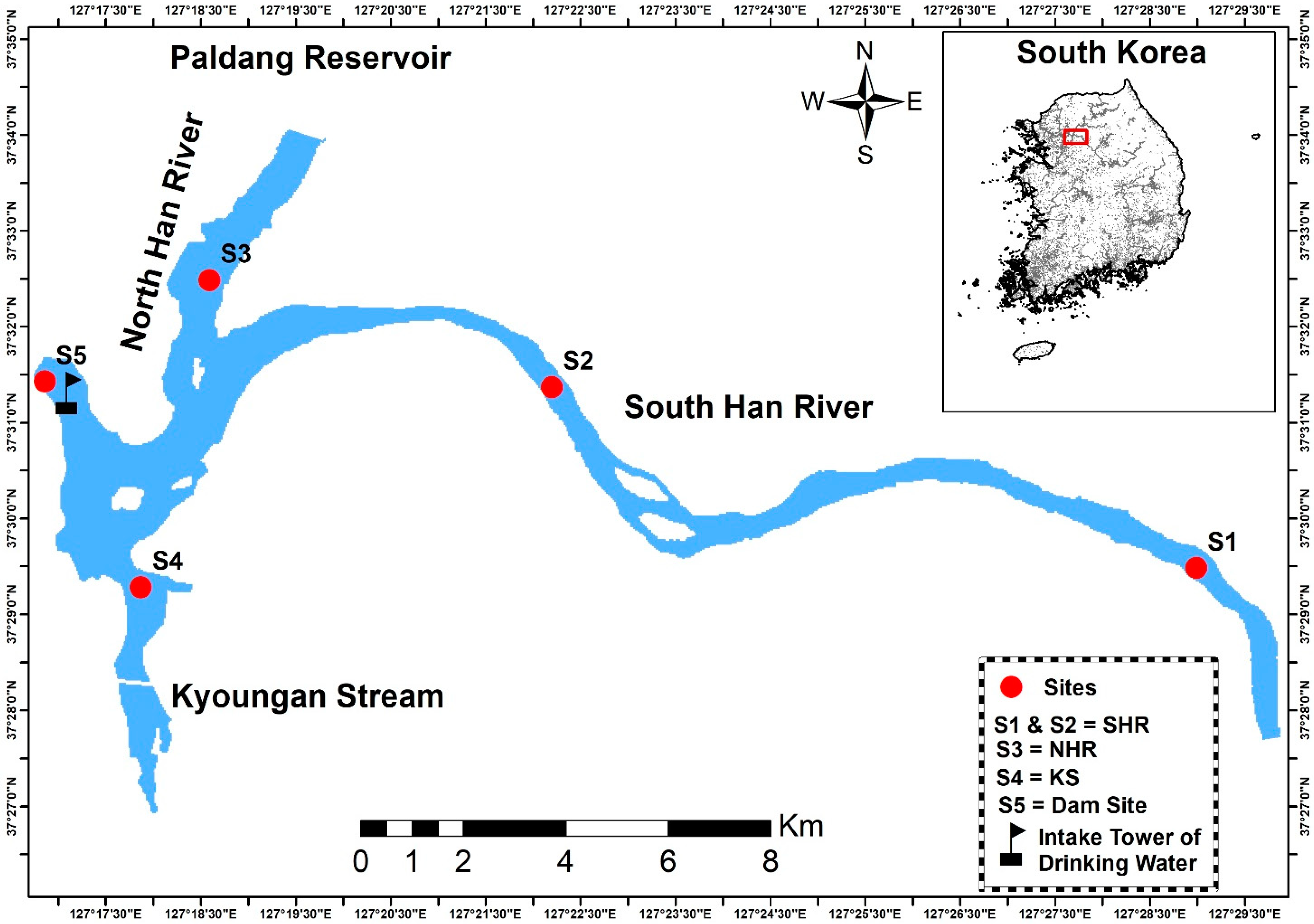
2.1. Study Area

The Paldang Reservoir is situated approximately 45 km northeast of Seoul and provides drinking water for 24 million people [14]. It has an area of 38.2 km2 and a volume of 250 × 106 m3 [11]. The mean and maximum depth of the reservoir is 6.5 m and 25 m, respectively [11]. Five reservoir sampling sites labelled S1–S5 were selected for this study. Sites S1 and S2 were located in the South Han River part of the reservoir. In contrast, S3, S4, and S5 were situated at the North Han River, Kyoungan Stream, and dam, respectively. The water intake tower for Paldang Reservoir is located at S5 (Figure 1). It receives water from three different sources, namely the Kyoungan Stream, South and North Han River, and directly affects the reservoir’s hydrodynamics and water quality [2,11,12,16]. About 95% of the reservoir’s water comes from the North and South Han Rivers, which have relatively good water quality [11]. In contrast with the two sources, Kyoungan Stream has a small flow rate and a lower water quality. The drinking water supply tower is located near Kyoungan Stream’s confluence and this significantly impacts drinking water quality (Figure 1).

2.2. Methodological Approach

This study solely depends on secondary data. To monitor the water quality parameters (WQPs: TP, BOD, and CHL-a) of a reservoir, several Landsat 5 TM images with band values were acquired and processed. Finally, regression analysis was carried out to establish a relationship between band values of Landsat images and in-situ measurements of WQPs. Figure 2 illustrates the methodological approach of this study.

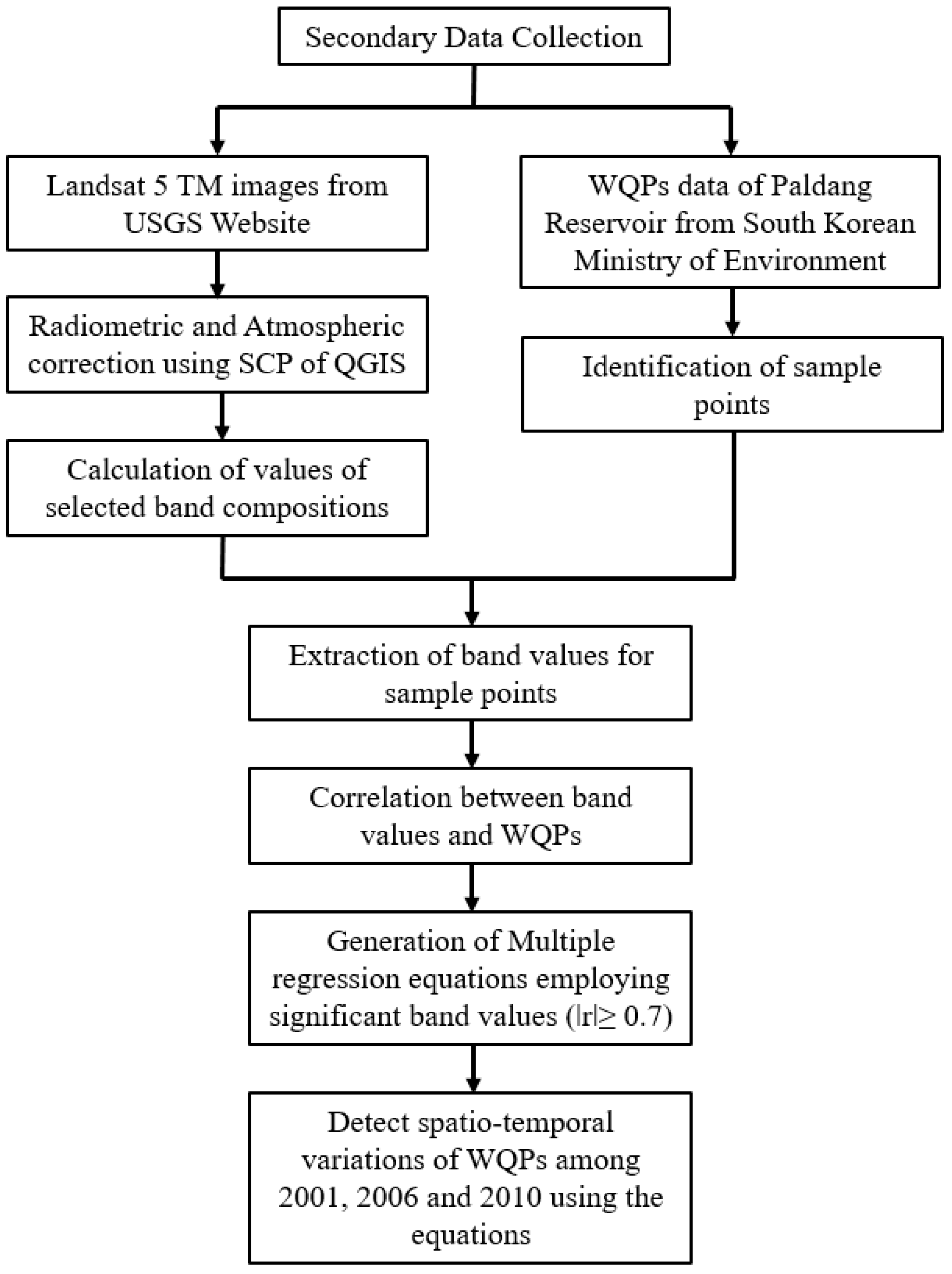
2.2.1. Acquisition and Processing of Satellite Data

A total of 19 images of Landsat 5 TM (path/row: 116/34 and 115/34) were downloaded from the United States Geological Survey (USGS) Website (https://earthexplorer.usgs.gov/, accessed on 26 April 2021). Seven images from the year 2001 (dated 11 January, 16 March, 17 April, 19 May, 15 September, 27 November, and 13 December), six images from 2006 (dated 25 January, 17 February, 14 March, 5 August, 13 September, and 18 December), and six images from 2010 (dated 5 February, 16 March, 24 September, 19 October, 11 November, and 29 December) were selected due to availability of cloud-free images. To make these raw images more suitable to use, appropriate radiometric and atmospheric corrections were carried out using the semi-automatic classification plugin (SCP) of QGIS. To remove the effect of haze, this plugin employs dark object subtraction (DOS) method. SCP is a widely used plugin for preprocessing satellite images [31,32]. SCP uses the spectral radiance scaling method to convert the digital number (DN) to top of atmosphere (TOA) reflectance in two steps [33]. The procedure is described in the following sections. At first, the spectral radiance at the sensor’s aperture 𝐿𝜆 (Wm−2 sr−1um−1) is measured from DN (Equation (1)) [34]:
Lλ = ML × Qcal + AL
where ML = Band-specific multiplicative rescaling factor from Landsat metadata (RADIANCE_MULT_BAND_x, where x is the band number), AL = Band-specific additive rescaling factor from Landsat metadata (RADIANCE_ADD_BAND_x, where x is the band number), Qcal = Quantized and calibrated standard product pixel values (DN). After that DOS, the image-based atmospheric correction is carried out in SCP to calculate land surface reflectance (Equation (3)) for each pixel by calculating path radiance (Equation (2)):
Lp = ML × DNmin + AL − 0.01 × ESUNλ × cosθs/(π × d2)
where, Lp = path radiance, DNmin = minimum DN value of the scene, d = Earth-Sun distance in astronomical units, ESUNλ = mean solar exo-atmospheric irradiances, θs = solar zenith angle in degrees, which is equal to θs = 90° − θe where θe is the Sun elevation:
ρ = [π × (Lλ Lp) × d2]/(ESUNλ × cosθs)
where, ρ = land surface reflectance, Lλ = spectral radiance at the sensor’s aperture, Lp = path radiance.

2.2.2. Assembling WQPs Data and Associated Band Values

The concentrations of different WQPs (TP, BOD, and CHL-a) of five sample collection points in Paldang Reservoir were collected from the South Korean Ministry of Environment for 2001, 2006, and 2010. These measurements are usually collected once a month. The dates of acquisition of satellite images were near the sampling days. A total of 95-pixel values for each band associated with these sample points were extracted from processed satellite images in the ArcGIS platform (Esri Inc., Redlands, CA, USA). For this analysis, four bands (blue, green, red and near infra-red) of Landsat 5 TM images were selected to extract, and a total of 32 band compositions were calculated in Microsoft Excel (Microsoft Office, Redmond, WA, USA).

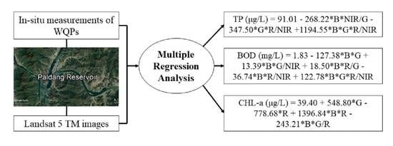
2.2.3. Development of Multiple Regression Equation between WQPs and Landsat Band Values

After arranging the data, outliers of the dataset were identified by plotting box-whisker plots (Supplementary File Figures S1–S3). These box-whisker plots have identified one outlier for BOD (3.5 mg/L), six for TP (123, 138, 140, 142, 228, 236 μg/L), four for CHL-a (49.1, 56.3, 71.9, 132 μg/L). For developing the empirical models, these outliers were omitted. Pearson’s coefficient of correlation (r) was calculated to find the strength of association among the band values and WQPs. To identify the significant band values, a threshold value of r was considered to be equal to or greater than 0.7, which represents strong correlation [21]. Multiple regression analysis was carried out in an online-based calculator to generate equations for each WQP. This analysis continued iteration until a significant p-value was obtained. This online-based calculator consideres all the assumptions of linear regression analysis (https://www.statskingdom.com/doc_linear_regression.html#multi, accessed on 26 April 2021). The assumptions are: (i) linearity—there is a linear relationship between the dependent variable, Y and the independent variables, Xi; (ii) residual normality; (iii) homoscedasticity (homogeneity of variance)—the variance of the residuals is constant and does not depend on the independent variables Xi; (iv) variables—the dependent variable, Y, should be continuous variable while the independent variables, Xi, should be continuous variables or ordinal variables; (v) multicollinearity—there is no perfect correlation among two or more independent variables, Xi.
To determine the efficiency of the generated models, root mean squared error (RMSE), root mean squared log error (RMSLE), mean relative error (MRE) and mean absolute error (MAE) were computed along with coefficient of determination (r2) and p-values. The following are the equations of RMSE, RMSLE, MRE and MAE. These equations can be applied to radiometrically and atmospherically corrected Landsat 5 TM images to predict specific water properties (TP, BOD and CHL-a):
R M S E = ( P i O i ) 2 n
R M S L E = ( log ( P i + 1 ) log ( O i + 1 ) ) 2 n
M R E = | P i O i 1 | n
M A E = | P i O i | n
where, Pi = predicted values of WQPs, Oi = observed values of WQPs, and n = sample size.

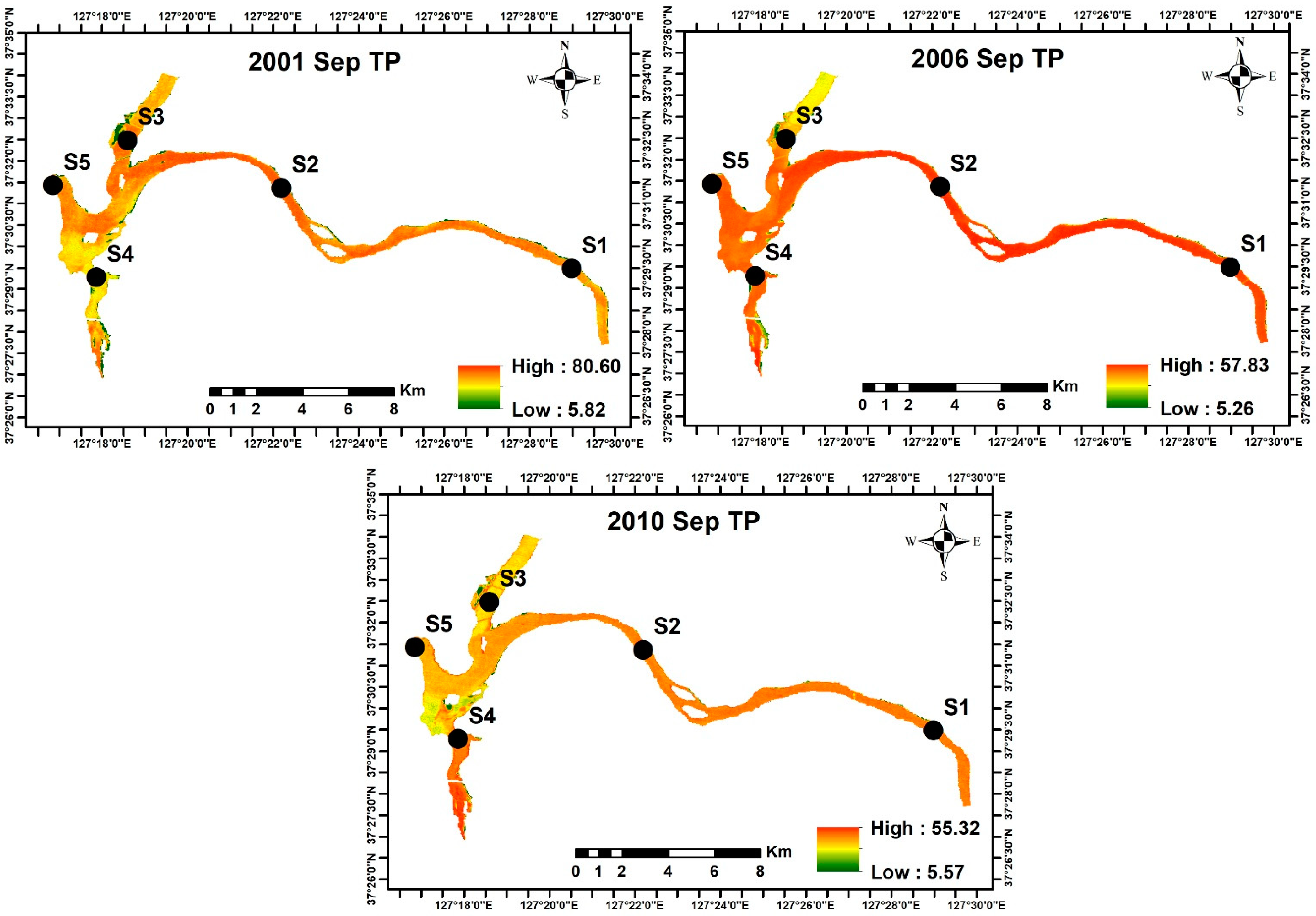
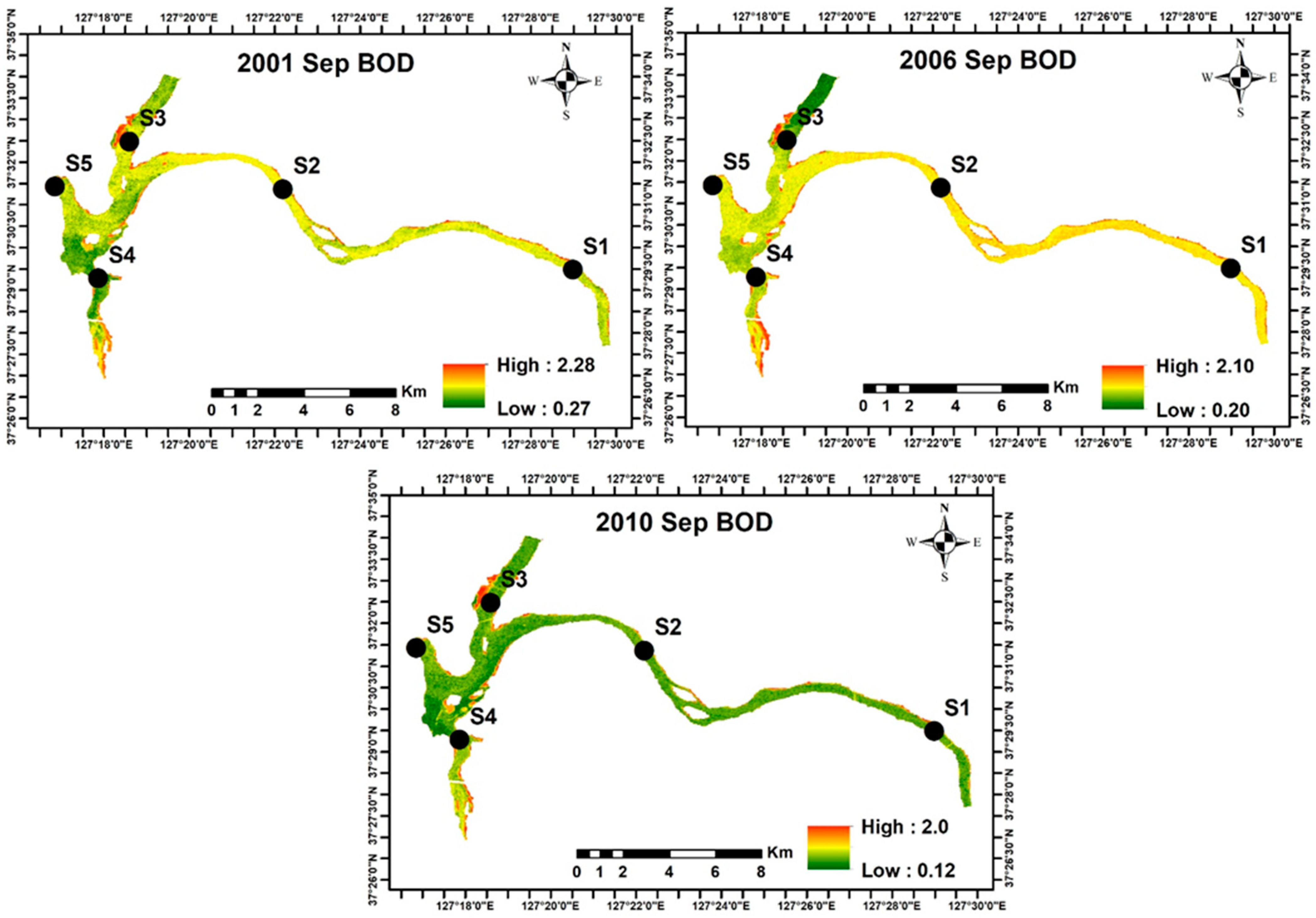
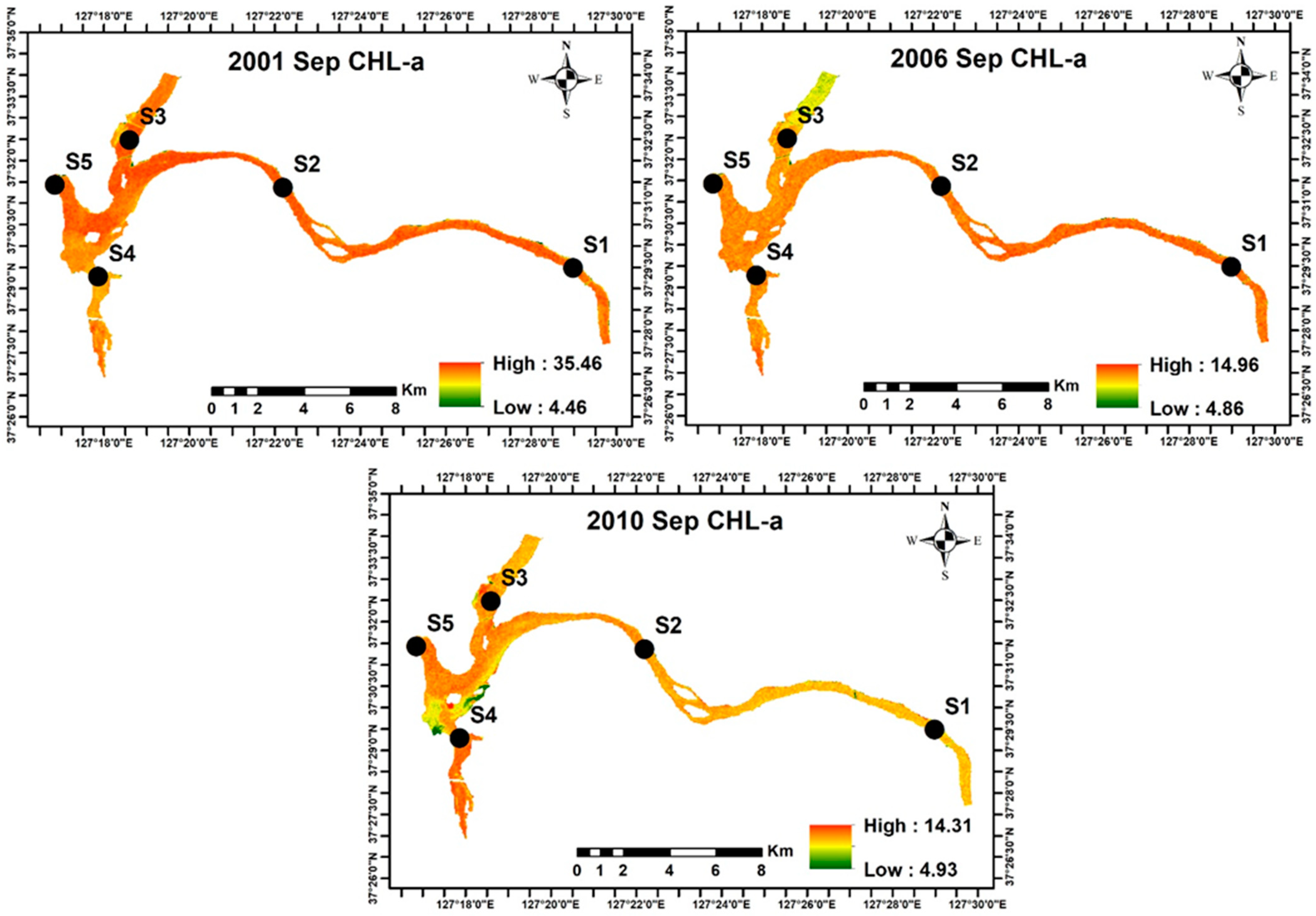
2.3. Spatio-Temporal Variation of WQPs

The spatio-temporal variation in WQPs of Paldang Reservoir for the years 2001, 2006, and 2010 were studied using the generated equations. Landsat 5 TM images of the month of September of these years were processed in SCP of QGIS, and the area of interest- Paldang Reservoir was extracted from the images. From their band values, values of WQPs were computed in Raster Calculator (Esri Inc., USA) and analyzed for the change detection study.

3. Results

3.1. Reservoir Conditions

The water quality parameters (TP, BOD, and CHL-a) of the Paldang Reservoir showed significant site variations (Table 1). The mean TP varied from 34.75–92.06 µgL−1 from sites S1–S5. Site S4 showed the highest TP (92.06 µgL−1) value compared to all sites due to the reception of wastewater from industry and household activities. Moreover, Site S4 is highly impacted by the Kyoungan Stream. Nürnberg [35] proposed that TP concentrations > 30 µgL−1 indicate a eutrophic reservoir. Mean TP levels above 30 µgL−1 at all sites were observed in this study. High BOD values suggest that organic matter pollution is linked to wastewater effluents. The mean BOD ranged from 1.05 to 1.72 mgL−1 in the Paldang Reservoir. Like TP, the highest BOD had been observed in Site S4 (1.72 mgL−1). It is well known that CHL-a is the primary indicator of eutrophication in the lentic system [5,36]. The mean CHL-a varied from 10.89 to 27.74 µgL−1. Nürnberg [35] proposed that eutrophic reservoir should be indicated by CHL-a concentrations greater than 9 µgL−1. Mean CHL-a concentrations at five sites were found above 9 µgL−1. Like TP and BOD, the highest CHL-a was also observed at site S4. Industrial and household wastewater and the Kyoungan Stream highly affect the water quality of site S4. Eun and Seok [11] and Mamun et al. [2] found that the water quality of the Kyoungan Stream is in poor condition compared to the South Han River (sites S1 and S2) and North Han River (Site S3), and this could have a major effect on the reservoir’s water quality.
A Pearson-based correlation analysis was used to identify the relationship among TP, BOD, and CHL-a (p < 0.05; Table 2). The BOD showed positive correlation with TP (r = 0.249) and CHL-a (r = 0.627). The positive correlation between BOD and TP suggests that nutrients (TP) flow into the Paldang Reservoir along with organic matter (BOD). The high positive correlation between BOD and CHL-a indicates that autochthonous organic matter production is primarily resulting from phytoplankton processes. CHL-a was positively related with TP (r = 0.375), which is the key factor regulating algal growth in the freshwater lentic system [5,9,10].

3.2. Relations of Band Compositions with TP, BOD, and CHL-a

Values of 32 band compositions and associated TP, BOD, and CHL-a concentrations were employed to compute correlation (r) values for Landsat 5 TM sensors. The band compositions and their allied r values are shown in Table 3. Only four bands (blue, green, red, and near-infrared) provide the visibly displayed water quality parameter spectral reflectiveness (0.4–0.9 μm); that is why we used these four bands to determine TP, BOD, and CHL-a [20]. TP is a significant factor in deciding eutrophication in freshwater systems. The TM bands’ correlation with TP ranged from −0.07 (B2/B4) to −0.79 (B1). Particularly, TP showed the strongest correlation with B1 (r = −0.79). The present findings have concurred with some previous studies [20]. BOD is the indicator of organic pollution in the aquatic systems. BOD and TM bands’ correlation varied from −0.15 (B1/B3) to −0.76 (B1*B3/B4). Like TP, BOD showed the highest correlation with B1 (r = −0.75) and B1*B3/B4 (r = −0.76). CHL-a is a good indicator of overall algal biomass in the aquatic systems. The present results showed a dynamic relation between TM bands and CHL-a. The correlation among TM bands and CHL-a ranged from 0.12 (B2/B3) to −0.79 (B1). Like TP and BOD, CHL-a showed the highest correlation with B1 (r = −0.79). From the r values, influential bands and band compositions have been identified to generate empirical models for TP, BOD, and CHL-a (marked in bold; Table 3).

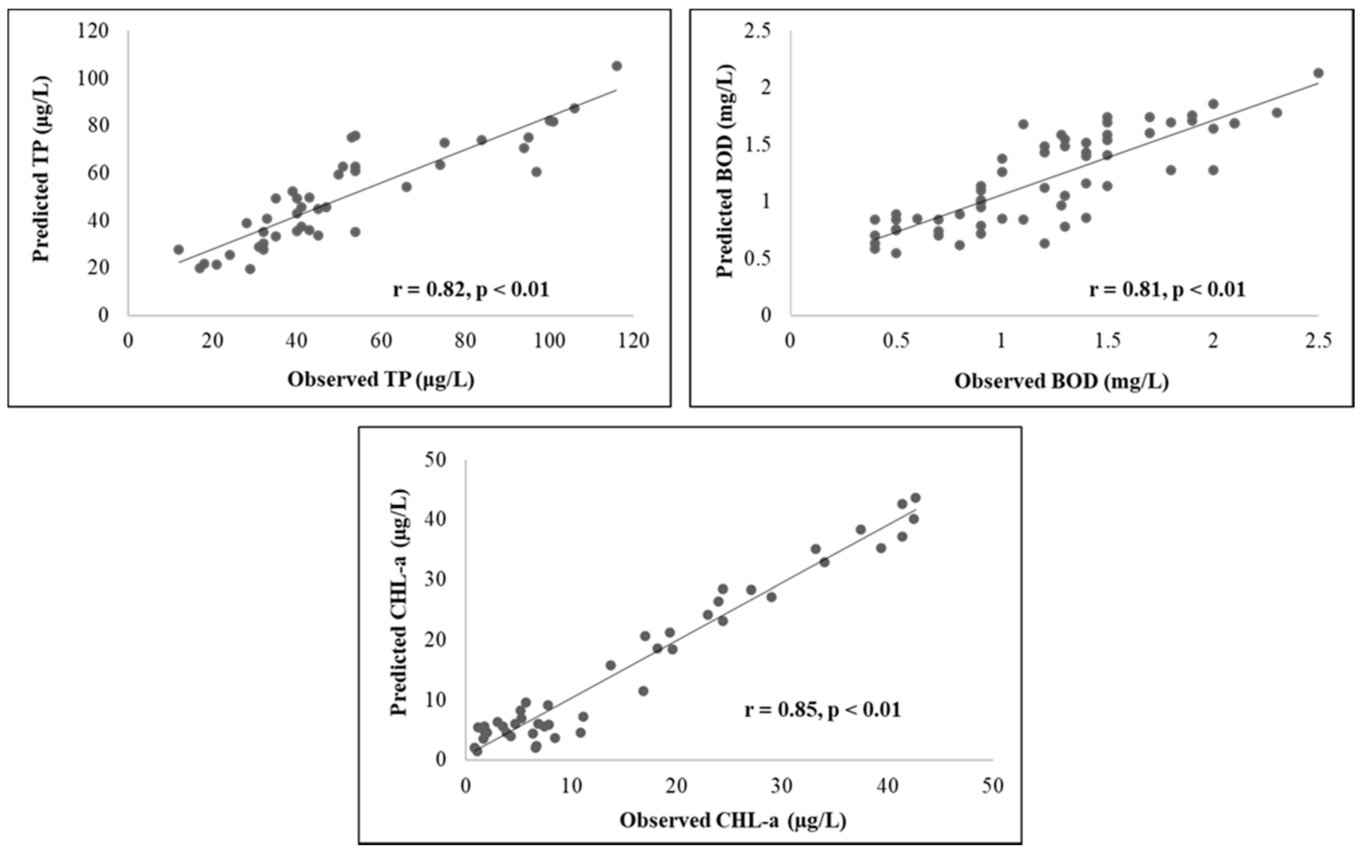
3.3. Empirical Model Development of TP, BOD, and CHL-a from Landsat 5 TM Data

Variables with high correlation values (|r| ≥ 0.70) have only been used to generate the empirical model for TP, BOD, and CHL-a (Table 4). The analysis was performed in an online-based calculator until a significant relationship was indicated by the p-value (p < 0.01). Due to an online-based calculator’s automatic iteration power, it is not easy to control the inclusion of any specific independent variables. The p-values for the model show that they have a significant relationship. The developed model using Landsat 5 TM images can detect TP 67% correctly while it was 65% and 72% for BOD and CHL-a, respectively (Table 4). The values of RMSE, RMSLE, MRE and MAE also depict the efficiency of developed models (Table 4). A more efficient TP, BOD, and CHL-a models from Landsat 5 TM can be developed using more sampling point data [21]. Considering our findings, further studies should be carried out with satellite sensors data to develop the empirical models of TP, BOD, and CHL-a. Scatter plots of the observed TP, BOD, and CHL-a data with predicted TP, BOD, and CHL-a values from the generated regression models are shown in Figure 3. For TP, the relationship between observed and predicted values displayed a correlation of 0.82 with p < 0.01. In contrast, it was 0.81 and 0.85 for BOD and CHL-a, respectively with p < 0.01.

3.4. Spatial and Temporal Patterns of Water Quality Parameters

The developed empirical models were applied to all study sites on the Paldang Reservoir to monitor spatio-temporal distributions of WQPs on 15 September 2001; 13 September 2006, and 24 September 2010, using Landsat 5 TM images (Figure 4, Figure 5 and Figure 6). Sites S1 and S2 are influenced by the South Han River, While S3 and S4 are affected by the North Han River and Kyoungan Stream. The TP concentration varied between 5.82 to 80.60 µgL−1 on 15 September 2001. The maximum TP concentrations gradually decreased from 2001 (80.60 µgL−1) to 2006 (57.83 µgL−1) and 2010 (55.32 µgL−1) in the Paldang Reservoir due to new treatment facilities in the sewage treatment plants and the development of water quality management strategies in the reservoirs (Figure 4). However, the TP concentrations were still in a eutrophic state in site S3 and S4 during 2006 and 2010. Like TP, the maximum BOD concentration also showed decreasing pattern from 2001 (2.28 mgL−1) to 2006 (2.10 mgL−1) and 2010 (2.0 mgL−1) (Figure 5). It indicates that the biological effluent treatment process may efficiently degrade the influent’s degradable organic matter [16]. The highest BOD level was also observed in S4 during 2010 September. Like TP and BOD, the maximum level of CHL-a was also showed a declining trend from 2001 (35.46 µgL−1) to 2006 (14.96 µgL−1) and 2010 (14.31 µgL−1) (Figure 6). During 2001 September, the entire reservoir showed a eutrophic state (>9 µgL−1) based on CHL-a concentration. Although the water quality is getting better in terms of TP, BOD, and CHL-a from 2001 to 2010, Site S3 and S4 are still facing some problems. The authors suggest that sites S3 and S4 should be taken under special consideration as S4 highly influences the intake tower water quality.

4. Discussion

The present study shows that remote sensing technology can be a handy tool to detect water quality parameters. Landsat data series are useful for monitoring the water quality of freshwater bodies. Paldang Reservoir has experienced significant water quality changes due to urbanization, land use change, and intensive agricultural farming [14,15,17]. The observed mean TP and CHL-a concentration at all sites in the Paldang Reservoir showed eutrophic conditions. This indicates a moderate risk of cyanobacterial exposure in the reservoir [37]. Previous studies stated that blooms of cyanobacteria are associated with eutrophic conditions in water bodies [36]. CHL-a is a good predictor of total phytoplankton biomass and monitoring CHL-a is a direct tool for semiquantitative estimation of cyanobacterial biomass in aquatic environments [2]. Previous studies of Paldang Reservoir have suggested that cyanobacterial blooms occur during the spring season and identified the following genera: Anabaena, Aphanocapsa, Chroococcus, Coelosphaerium, Dactylococcopsis, Microcystis, Merismopedia, Phormidium, Oscillatoria, and Pseudoanabaen [2,16,18]. In addition, TP, BOD, and CHL-a levels at site S4 were constantly elevated. The water quality of site S4 is heavily impacted by industrial and domestic wastewater and the Kyoungan Stream. Eun and Seok [11] and Mamun et al. [2] found that the water quality of the Kyoungan Stream is in poor condition in comparison to the Southern Han River (Sites S1 and S2) and Northern Han River (Site S3) based on nutrients, organic matter and algal chlorphyll. It could have significant effects on the reservoir’s water quality.
Variation in TP, BOD, and CHL-a concentrations of the Paldang Reservoir was prominent during the pre-monsoon, monsoon, and post-monsoon seasons [18]. TP concentrations were higher during the monsoon period due to intense precipitation, while BOD and CHL-a level at Paldang Reservoir was highest in the spring period [2,18]. The summer monsoon significantly influences the nutrient, organic matter, and algal chlorophyll in the Korean reservoirs [5,16,38]. Organic matter in aquatic systems may come from allochthonous or autochthonous sources. Allochthonous organic matter enters into the environment during precipitation events, while algae produce autochthonous organic matter by photosynthesis [18]. It was noticeable that 69% of the total organic matter was allochthonous in the Paldang Reservoir during monsoon season [18]. Inversely, during winter and spring, a high load of autochthonous organic matter had observed because of low flow rates and high water residence time [16]. Previous research on Paldang Reservoir indicated that 73% of autochthonous organic matter loading happens during the spring [16,18]. The high-level organic matter during spring corresponds to algae’s maximum production [18]. It suggests that autochthonous production by algae (CHL-a) is dire to accumulate organic matter in the reservoir during spring; hence, the threat to the reservoir’s water quality is highest in spring [18].
The water quality of the Paldang Reservoir varied from site to site and season to season due to climatic factors and anthropogenic activities. Since climatic conditions are uncontrollable, anthropogenic impacts should be kept to a minimum. For that reason, regular monitoring of water quality parameters is essentially mandatory. Traditional monitoring approaches are time-intensive, laborious, and cannot provide an overview of water quality at a broader scale [1,19].
On the other hand, satellite remote sensing is presently one of the most potent and reliable approaches for monitoring and managing water quality [4,20,21]. This study has confirmed the applicability of Landsat 5 TM to identify and map the water quality parameters in the reservoir. The developed empirical models by multiple linear regression analysis can identify TP 67%, BOD 65%, and CHL-a 72% accurately from Landsat 5 TM images. As shown in Table 4, blue*near-infrared/green (B1*B4/B2), green*red/near-infrared (B2*B3/B4), and blue*green*red/near-infrared (B1*B2*B3/B4) bands and band ratios are the significant predictors for TP concentrations in Paldang Reservoir. Previous studies also found that three visible bands (blue, green, and red) and NIR bands and their ratios are suitable for estimating TP concentrations in freshwater systems [4,20]. blue*green (b1*b2), blue*green/near-infrared(b1*b2/b4), blue*Red/Green (B1*B3/B2), blue*red/near-infrared (B1*B3/B4), blue*green*red/near-infrared (B1*B2*B3/B4) bands and band ratios are the significant predictors for BOD concentrations in the reservoir. Quibell [39] reported that the NIR and red bands ratio were good predictors of CHL-a concentration in waters. Also, other bands and band ratios are good indicators of CHL-a [40]. The present result indicated that CHL-a was better explained by the green (B2), red (B3), blue*red (B1*B3) and blue*green/red (B1*B2/B3) bands and band ratios.

5. Conclusions

Nutrient and organic pollution and algal blooms regulate water quality in freshwater systems. For this reason, it is essential to develop a cost-effective remote sensing monitoring tool to estimate the water quality parameters for maintaining an effective water management system. The present study has successfully established Landsat 5 TM data’s applicability to detect TP, BOD, and CHL-a for the surface water of Paldang Reservoir (Korea). The results showed that TP, BOD, and CHL-a are closely related to the Landsat 5 surface reflectance band values. TP (r = −0.79) and CHL-a (r = −0.79) showed the highest relations with B1 (blue) band. By contrast, BOD showed the highest negative correlation with B1 (blue) (r = −0.75) and B1*B3/B4 (blue*red/near-infrared) bands (r = −0.76). The developed empirical models of Landsat 5 TM data can estimate TP, BOD, and CHL-a correctly by around 67%, 65%, and 72%, respectively, for the reservoir. The results presented here revealed that the surface water quality of the reservoir varied from site to site. The water quality of sites S3 and S4 are affected by anthropogenic factors, which significantly impact reservoir’s water quality. Considering the present findings, we should take a particular account for site S3 and S4 to maintain the water quality. The present developed models and methods could be applied to other Korean reservoirs for validation.

Supplementary Materials

The following are available online at https://0-www-mdpi-com.brum.beds.ac.uk/article/10.3390/rs13122256/s1. Figure S1 Outlier detection for BOD; Figure S2 Outlier detection for TP; Figure S3 Outlier detection for CHL-a.

Author Contributions

Conceptualization, M.M.; methodology, M.M. and J.F.; software, M.M. and J.F.; validation, M.M. and J.F.; formal analysis, M.M. and J.F.; resources, M.M. and J.F.; data curation, M.M.; writing—original draft preparation, M.M. and J.F.; writing—review and editing, M.M., J.F. and K.-G.A.; visualization, M.M. and J.F.; supervision, K.-G.A.; project administration, K.-G.A.; funding acquisition, K.-G.A. All authors have read and agreed to the published version of the manuscript.

Funding

This research was funded by the Korea Environmental Industry & Technology Institute (KEITI) project (Project:2020-1008-01) “Development of Longitudinal Connectivity Evaluation System, Based on the Fish Movement”.

Institutional Review Board Statement

Not applicable.

Informed Consent Statement

Not applicable.

Data Availability Statement

The datasets presented in this study are available on reasonable request from the corresponding author.

Acknowledgments

The authors would like to acknowledge the Korea Environmental Industry & Technology Institute (KEITI) for their assistance.

Conflicts of Interest

The authors declare no conflict of interest.

References

  1. Mushtaq, F.; Nee Lala, M.G. Remote estimation of water quality parameters of Himalayan lake (Kashmir) using Landsat 8 OLI imagery. Geocarto Int. 2017, 32, 274–285. [Google Scholar] [CrossRef]
  2. Mamun, M.; Kim, J.Y.; An, K.-G. Multivariate Statistical Analysis of Water Quality and Trophic State in an Artificial Dam Reservoir. Water 2021, 13, 186. [Google Scholar] [CrossRef]
  3. Li, Y.; Zhang, Y.; Shi, K.; Zhu, G.; Zhou, Y.; Zhang, Y.; Guo, Y. Monitoring spatiotemporal variations in nutrients in a large drinking water reservoir and their relationships with hydrological and meteorological conditions based on Landsat 8 imagery. Sci. Total Environ. 2017, 599, 1705–1717. [Google Scholar] [CrossRef]
  4. Torbick, N.; Hession, S.; Hagen, S.; Wiangwang, N.; Becker, B.; Qi, J. Mapping inland lake water quality across the Lower Peninsula of Michigan using Landsat TM imagery. Int. J. Remote Sens. 2013, 34, 7607–7624. [Google Scholar] [CrossRef]
  5. Mamun, M.; Kwon, S.; Kim, J.E.; An, K.G. Evaluation of algal chlorophyll and nutrient relations and the N:P ratios along with trophic status and light regime in 60 Korea reservoirs. Sci. Total Environ. 2020, 741, 140451. [Google Scholar] [CrossRef] [PubMed]
  6. Smith, V.H. Responses of estuarine and coastal marine phytoplankton to nitrogen and phosphorus enrichment. Limnol. Oceanogr. 2006, 51, 377–384. [Google Scholar] [CrossRef] [Green Version]
  7. Rabalais, N.N.; Turner, R.E.; Díaz, R.J.; Justić, D. Global change and eutrophication of coastal waters. ICES J. Mar. Sci. 2009, 66, 1528–1537. [Google Scholar] [CrossRef]
  8. Li, Y.; Cao, W.; Su, C.; Hong, H. Nutrient sources and composition of recent algal blooms and eutrophication in the northern Jiulong River, Southeast China. Mar. Pollut. Bull. 2011, 63, 249–254. [Google Scholar] [CrossRef]
  9. Jones, J.R.; Obrecht, D.V.; Thorpe, A.P. Chlorophyll maxima and chlorophyll: Total phosphorus ratios in Missouri reservoirs. Lake Reserv. Manag. 2011, 27, 321–328. [Google Scholar] [CrossRef] [Green Version]
  10. Atique, U.; An, K.G. Landscape heterogeneity impacts water chemistry, nutrient regime, organic matter and chlorophyll dynamics in agricultural reservoirs. Ecol. Indic. 2020, 110, 105813. [Google Scholar] [CrossRef]
  11. Eun, H.N.; Seok, S.P. A hydrodynamic modeling study to determine the optimum water intake location in Lake Paldang, Korea. J. Am. Water Resour. Assoc. 2005, 41, 1315–1332. [Google Scholar] [CrossRef]
  12. Boopathi, T.; Wang, H.; Lee, M.-D.; Ki, J.-S. Seasonal Changes in Cyanobacterial Diversity of a Temperate Freshwater Paldang Reservoir (Korea) Explored by using Pyrosequencing. Environ. Biol. Res. 2018, 36, 424–437. [Google Scholar] [CrossRef]
  13. MOE. (ECOREA) Environmental Review 2015; Ministry of Environment: Sejong City, Korea, 2015; Volume 1. [Google Scholar]
  14. Lee, J.E.; Youn, S.J.; Byeon, M.; Yu, S.J. Occurrence of cyanobacteria, actinomycetes, and geosmin in drinking water reservoir in Korea: A case study from an algal bloom in 2012. Water Sci. Technol. Water Supply 2020, 20, 1862–1870. [Google Scholar] [CrossRef]
  15. Kim, D.W.; Min, J.H.; Yoo, M.; Kang, M.; Kim, K. Long-term effects of hydrometeorological and water quality conditions on algal dynamics in the Paldang dam watershed, Korea. Water Sci. Technol. Water Supply 2014, 14, 601–608. [Google Scholar] [CrossRef]
  16. Park, H.K.; Cho, K.H.; Won, D.H.; Lee, J.; Kong, D.S.; Jung, D. Il Ecosystem responses to climate change in a large on-river reservoir, Lake Paldang, Korea. Clim. Chang. 2013, 120, 477–489. [Google Scholar] [CrossRef]
  17. Youn, S.J.; Kim, H.N.; Yu, S.J.; Byeon, M.S. Cyanobacterial occurrence and geosmin dynamics in Paldang Lake watershed, South Korea. Water Environ. J. 2020, 1–10. [Google Scholar] [CrossRef]
  18. Park, H.K.; Byeon, M.S.; Shin, Y.N.; Jung, D. Il Sources and spatial and temporal characteristics of organic carbon in two large reservoirs with contrasting hydrologic characteristics. Water Resour. Res. 2009, 45, 1–12. [Google Scholar] [CrossRef]
  19. Khattab, M.F.O.; Merkel, B.J. Application of landsat 5 and landsat 7 images data for water quality mapping in Mosul Dam Lake, Northern Iraq. Arab. J. Geosci. 2014, 7, 3557–3573. [Google Scholar] [CrossRef]
  20. Lim, J.; Choi, M. Assessment of water quality based on Landsat 8 operational land imager associated with human activities in Korea. Environ. Monit. Assess. 2015, 187, 1–17. [Google Scholar] [CrossRef]
  21. Ferdous, J.; Rahman, M.T.U. Developing an empirical model from Landsat data series for monitoring water salinity in coastal Bangladesh. J. Environ. Manag. 2020, 255, 109861. [Google Scholar] [CrossRef]
  22. Kumar, V.; Sharma, A.; Chawla, A.; Bhardwaj, R.; Thukral, A.K. Water quality assessment of river Beas, India, using multivariate and remote sensing techniques. Environ. Monit. Assess. 2016, 188, 1–10. [Google Scholar] [CrossRef]
  23. Zhang, Y.; Zhang, Y.; Shi, K.; Zhou, Y.; Li, N. Remote sensing estimation of water clarity for various lakes in China. Water Res. 2021, 192. [Google Scholar] [CrossRef]
  24. Zhou, W.; Wang, S.; Zhou, Y.; Troy, A. Mapping the concentrations of total suspended matter in Lake Taihu, China, using Landsat-5 TM data. Int. J. Remote Sens. 2006, 27, 1177–1191. [Google Scholar] [CrossRef]
  25. Brezonik, P.; Menken, K.D.; Bauer, M. Landsat-based remote sensing of lake water quality characteristics, including chlorophyll and colored dissolved organic matter (CDOM). Lake Reserv. Manag. 2005, 21, 373–382. [Google Scholar] [CrossRef]
  26. Miller, H.; Sexton, N.; Koontz, L.; Loomis, J.; Koontz, S.; Hermans, C. The Users, Uses, and Value of Landsat and Other Moderate-Resolution Satellite Imagery in the United States—Executive Report; U.S. Geological Survey: Reston, VA, USA, 2011.
  27. Wu, C.; Wu, J.; Qi, J.; Zhang, L.; Huang, H.; Lou, L.; Chen, Y. Empirical estimation of total phosphorus concentration in the mainstream of the Qiantang River in China using Landsat TM data. Int. J. Remote Sens. 2010, 31, 2309–2324. [Google Scholar] [CrossRef]
  28. Gholizadeh, M.H.; Melesse, A.M.; Reddi, L. A comprehensive review on water quality parameters estimation using remote sensing techniques. Sensors 2016, 16, 1298. [Google Scholar] [CrossRef] [PubMed] [Green Version]
  29. Gholizadeh, M.H. Water Quality Modelling Using Multivariate Statistical Analysis and Remote Sensing in South Florida. Ph.D. Thesis, Florida International University, Miami, FL, USA, 2016. [Google Scholar]
  30. Nas, B.; Ekercin, S.; Karabörk, H.; Berktay, A.; Mulla, D.J. An application of landsat-5TM image data for water quality mapping in Lake Beysehir, Turkey. Water Air Soil Pollut. 2010, 212, 183–197. [Google Scholar] [CrossRef]
  31. Ghorai, D.; Mahapatra, M. Correction to: Extracting Shoreline from Satellite Imagery for GIS Analysis. Remote Sens. Earth Syst. Sci. 2020, 3, 23. [Google Scholar] [CrossRef] [Green Version]
  32. Lehmann, J.R.K.; Prinz, T.; Ziller, S.R.; Thiele, J.; Heringer, G.; Meira-Neto, J.A.A.; Buttschardt, T.K. Open-source processing and analysis of aerial imagery acquired with a low-cost Unmanned Aerial System to support invasive plant management. Front. Environ. Sci. 2017, 5, 1–16. [Google Scholar] [CrossRef] [Green Version]
  33. Rahman, M.T.U.; Ferdous, J. Detection of Environmental Degradation of Satkhira District, Bangladesh Through Remote Sensing Indices. In GCEC 2017; Pradhan, B., Ed.; Lecture Notes in Civil Engineering; Springer: Singapore, 2019; Volume 9, pp. 1053–1066. ISBN 9789811080166. [Google Scholar]
  34. Congedo, L. Semi-Automatic Classification Plugin User Manual Release 5.3.6.1; RoMEO: Paterson, NJ, USA, 2017. [Google Scholar]
  35. Nürnberg, G.K. Trophic state of clear and colored, soft- and hardwater lakes with special consideration of nutrients, anoxia, phytoplankton and fish. Lake Reserv. Manag. 1996, 12, 432–447. [Google Scholar] [CrossRef]
  36. Carlson, R.E.; Havens, K.E. Simple graphical methods for the interpretation of relationships between trophic state variables. Lake Reserv. Manag. 2005, 21, 107–118. [Google Scholar] [CrossRef]
  37. WHO. Guidelines for Drinking Water Quality: Management of Cyanobacteria in Drinking Water Suppliers Information for Regulators and Water Suppliers, 4th ed.; World Health Organization: Geneva, Switzerland, 2011. [Google Scholar]
  38. Jung, S.; Shin, M.; Kim, J.; Eum, J.; Lee, Y.; Lee, J.; Choi, Y.; You, K.; Owen, J.; Kim, B. The effects of Asian summer monsoons on algal blooms in reservoirs. Inland Waters 2016, 6, 406–413. [Google Scholar] [CrossRef]
  39. Quibell, G. The effect of suspended sediment on reflectance from freshwater algae. Int. J. Remote Sens. 1991, 12, 177–182. [Google Scholar] [CrossRef]
  40. Kloiber, S.M.; Brezonik, P.L.; Olmanson, L.G.; Bauer, M.E. A procedure for regional lake water clarity assessment using Landsat multispectral data. Remote Sens. Environ. 2002, 82, 38–47. [Google Scholar] [CrossRef]
Figure 1. The map showing the study sites of Paldang Reservoir.
Remotesensing 13 02256 g001
Figure 2. Methodological flow chart of the study.
Remotesensing 13 02256 g002
Figure 3. The relationship among observed and predicted TP, BOD and CHL-a for Landsat 5 TM (TP: Total Phosphorus, BOD: Biological Oxygen Demand, and CHL-a: Chlorophyll-a).
Remotesensing 13 02256 g003
Figure 4. Spatial and temporal pattern of total phosphorus (TP) on September 2001, 2006 and 2010.
Remotesensing 13 02256 g004
Figure 5. Spatial and temporal pattern of biological oxygen demand (BOD) on September 2001, 2006 and 2010.
Remotesensing 13 02256 g005
Figure 6. Spatial and temporal pattern of chlorophyll-a (CHL-a) on September 2001, 2006 and 2010.
Remotesensing 13 02256 g006
Table 1. Summary statistics of Total Phosphorus (TP), Biological Oxygen Demand (BOD) and Chlorophyll-a (CHL-a) in Paldang Reservoir.
SitesTP (μg/L)
Mean ± SD
(Min−Max)
BOD (mg/L)
Mean ± SD
(Min−Max)
CHL-a (µg/L)
Mean ± SD
(Min−Max)
S150.93 ± 29.511.15 ± 0.5613.61 ± 6.16
(28–142)(0.4–2)(1.1–49.1)
S252.81 ± 27.351.31 ± 0.6115.37 ± 12.14
(29–140)(0.4–2.3)(0.9–37.5
S334.75 ± 22.941.05 ± 0.3510.89 ± 6.83
(11–100)(0.4–1.5)(1.2–24.4)
S492.06 ± 66.661.72 ± 0.6827.74 ± 14.37
(11–236)(0.8–3.5)(3–132)
S543.25 ± 28.181.18 ± 0.3716.71 ± 11.52
(12–116)(0.7–1.9)(5.3–42.5)
Table 2. Pearson correlation among total phosphorus (TP), biological oxygen demand (BOD) and chlorophyll-a (CHL-a).
Variablesr Valuep
BODTP0.2490.02
BODCHL-a0.627<0.001
TPCHL-a0.375<0.001
Table 3. Correlation matrix values for different band compositions of Landsat 5 TM with TP, BOD and CHL-a (B1: Blue, B2: Green, B3: Red, B4: NIR-Near-Infrared, TP: Total Phosphorus, BOD: Biological Oxygen Demand, CHL-a: Chlorophyll-a, influential bands and band compositions have been (r ≥ 0.7) marked in bold.
Band Compositionr-Values
TPBODCHL-a
B1−0.79−0.75−0.79
B2−0.76−0.74−0.76
B3−0.74−0.71−0.75
B4−0.68−0.60−0.53
B1*B2−0.70−0.71−0.72
B1*B3−0.68−0.67−0.70
B1*B4−0.65−0.63−0.62
B2*B3−0.66−0.65−0.68
B2*B4−0.63−0.62−0.56
B3*B4−0.61−0.58−0.58
B1*B2*B3−0.58−0.57−0.61
B1*B2*B4−0.57−0.55−0.55
B1*B3*B4−0.55−0.52−0.53
B2*B3*B4−0.54−0.50−0.51
B1/B2−0.42−0.25−0.39
B1/B3−0.20−0.15−0.28
B1/B4−0.28−0.36−0.33
B2/B30.310.180.12
B2/B4−0.07−0.27−0.18
B3/B4−0.27−0.41−0.24
B1*B2/B3−0.76−0.73−0.75
B1*B2/B4−0.72−0.74−0.72
B1*B3/B2−0.78−0.73−0.78
B1*B3/B4−0.78−0.76−0.75
B1*B4/B2−0.72−0.61−0.63
B1*B4/B3−0.73−0.63−0.58
B2*B3/B1−0.65−0.64−0.65
B2*B3/B4−0.75−0.74−0.72
B1*B2*B3/B4−0.71−0.71−0.72
B1*B2*B4/3−0.67−0.66−0.59
B1*B3*B4/2−0.63−0.59−0.60
B2*B3*B4/B1−0.59−0.55−0.51
Table 4. Linear equations for Landsat 5 TM to detect TP, BOD and CHL-a of Paldang Reservoir (B: Blue, G: Green, R: Red, NIR: Near-Infrared, TP: Total Phosphorus, BOD: Biological Oxygen Demand, CHL-a: Chlorophyll-a, WQPs: Water Quality Parameters).
SensorWQPsEquationsR2pRMSERMSLEMREMAE
Landsat 5 TMTP=91.01 − 268.22*B*NIR/G − 347.50*G*R/NIR + 1194.55*B*G*R/NIR0.67<0.0130.40.0720.113.39
BOD=1.83 − 127.38*B*G + 13.39*B*G/NIR + 18.50*B*R/G − 36.74*B*R/NIR + 122.78*B*G*R/NIR0.65<0.010.080.0580.250.23
CHL-a=39.40 + 548.80*G − 778.68*R + 1396.84*B*R − 243.21*B*G/R0.72<0.014.90.1550.341.41
Publisher’s Note: MDPI stays neutral with regard to jurisdictional claims in published maps and institutional affiliations.

