Article

DeepIndices: Remote Sensing Indices Based on Approximation of Functions through Deep-Learning, Application to Uncalibrated Vegetation Images

Agroécologie, AgroSup Dijon, INRA, University of Bourgogne-Franche-Comté, F-21000 Dijon, France
*
Author to whom correspondence should be addressed.
Remote Sens. 2021, 13(12), 2261; https://0-doi-org.brum.beds.ac.uk/10.3390/rs13122261
Submission received: 2 April 2021 / Revised: 7 May 2021 / Accepted: 16 May 2021 / Published: 9 June 2021
(This article belongs to the Special Issue Remote Sensing for Precision Agriculture)

Abstract

:
The form of a remote sensing index is generally empirically defined, whether by choosing specific reflectance bands, equation forms or its coefficients. These spectral indices are used as preprocessing stage before object detection/classification. But no study seems to search for the best form through function approximation in order to optimize the classification and/or segmentation. The objective of this study is to develop a method to find the optimal index, using a statistical approach by gradient descent on different forms of generic equations. From six wavebands images, five equations have been tested, namely: linear, linear ratio, polynomial, universal function approximator and dense morphological. Few techniques in signal processing and image analysis are also deployed within a deep-learning framework. Performances of standard indices and DeepIndices were evaluated using two metrics, the dice (similar to f1-score) and the mean intersection over union (mIoU) scores. The study focuses on a specific multispectral camera used in near-field acquisition of soil and vegetation surfaces. These DeepIndices are built and compared to 89 common vegetation indices using the same vegetation dataset and metrics. As an illustration the most used index for vegetation, NDVI (Normalized Difference Vegetation Indices) offers a mIoU score of 63.98% whereas our best models gives an analytic solution to reconstruct an index with a mIoU of 82.19%. This difference is significant enough to improve the segmentation and robustness of the index from various external factors, as well as the shape of detected elements.

Graphical Abstract

1. Introduction

An important advance in the field of earth observation is the discovery of spectral indices, they have proved their effectiveness in surface description. Several studies have been conducted using remote sensing indices, often applied to a specific field of study like evaluations of vegetation cover, vigor, or growth dynamics [1,2,3,4] for precision agriculture using multi-spectral sensors. Some spectral indices have been developed using RGB or HSV color space to detect vegetation from ground cameras [5,6,7]. Remote sensing indices can also be used for other surfaces analysis like water, road, snow [8] cloud [9] or shadow [10].
There are two main problems with these indices. Firstly they are almost all empirically defined, although the selection of wavelengths comes from observation, like NDVI for vegetation indices. It is possible to obtain better spectral combinations or equations to characterize a surface with specific acquisitions parameters. It is important to optimize upstream the index, as the data transformation leads to a loss of essential information and features for classification [11]. Most studies have tried to optimize some parameters of existing indices. For example, an optimization of NDVI ( N I R R e d ) / ( N I R + R e d ) was proposed by [12] under the name of WDRVI (Wide Dynamic Range Vegetation Index) ( α N I R R e d ) / ( α N I R + R e d ) . The author tested different values for α between 0 and 1. The ROC curve was used to determine the best coefficient for a given ground truth. Another optimized NDVI was designed and named EVI (Enhanced Vegetation Index). It takes into account the blue band for atmospheric resistance by including various parameters G ( N I R R e d ) / ( N I R + C 1 R e d C 2 B l u e + L ) , where G , L are respectively the gain factor and the canopy background adjustment, in addition the coefficients C 1 , C 2 are used to compensate for the influence of clouds and shadows. Many other indices can be found in an online database of indices (IDB: www.indexdatabase.de accessed 10 August 2019) [10] including the choice of wavelengths and coefficients depending on the selected sensors or applications. But none of the presented indices are properly optimized. Thus, in the standard approach, the best index is determined by testing all available indices against the spectral bands of the selected sensor with a Pearson correlation between these indices and a ground truth [13,14]. Furthermore, correlation is not the best estimator because it neither considers the class ratio nor the shape of the obtained segmentation and may again result in a non-optimal solution for a specific segmentation task. Finally, these indices are generally not robust because they are still very sensitive to shadows [11]. For vegetation, until recently, all of the referenced popular indices were man-made and used few spectral bands (usually NIR, red, sometimes blue or RedEdge).
The second problem with standard indices is that they work with reflectance-calibrated data. Three calibration methods can be used in proximal-sensing. (i) The first method use an image taken before acquisition containing a color patch as a reference [15,16], and is used for correction. The problem with this approach is that if the image is partially shaded, the calibration is only relevant on the non-shaded part. Moreover ideally the reference must be updated to reduce the interference of weather change on the spectrum measurement, which is not always possible since it’s a human task. (ii) An other method is the use of an attached sunshine sensor [17], which also requires calibration but does not allow to correct a partially shaded image. (iii) The last method is the use of a controlled lighting environment [18,19], e.g., natural light is suppressed by a curtain and replaced by artificial lighting. All of these approaches are sometimes difficult to implement for automatic, outdoor use, and moreover in real time like detecting vegetation while a tractor is driving through a crop field.
In recent years, machine learning algorithms have been increasingly used to improve the definition of presented indices in the first main problem. Some studies favor the use of multiple indices and advanced classification techniques (RandomForest, Boosting, DecisionTree, etc.) [4,20,21,22,23,24]. Another study has proposed to optimize the weights in an NDVI equation form based on a genetic algorithm [25] but does not optimize the equation forms. An other approach has been proposed to automatically construct a vegetation index using a genetic algorithm [26]. They optimize the equation forms by building a set of arithmetic graphs with mutations, crossovers and replications to change the shape of each equation during learning but it does not take into account the weights, since it’s use calibrated data. Finally, with the emergence of deep learning, current studies try to adapt popular CNN architectures (UNet, AlexNet, etc.) to earth observation applications: [27,28,29,30].
However there is no study that optimize both the equation forms and spectral bands weights. The present study explicitly optimize both of them by looking for a form of remote sensing indices by learning weights in functions approximators. These functions approximators will then reconstruct any equation forms of the desired remote sensing index for a given acquisition system. To solve the presented second problem, this study evaluates the functions approximators on an uncalibrated dataset containing various acquisition conditions. This is not a common approach but can be found in the literature [31,32]. This will lead to creating indices that do not require data calibration. The deep learning framework has been used as a general regression toolkit. Thus, several CNN function approximators architectures are proposed. DeepIndices is presented as a regression problem, which is totally new, as is the use of signal and image processing.

2. Material and Data

2.1. Instrument Details

The images were acquired with the Airphen (Hyphen, Avignon, France) six-band multi-spectral camera (Figure 1). This is a multi-spectral scientific camera developed by agronomists for agricultural applications. It can be integrated into different types of platforms such as drones, phenotyping robots, etc.
The camera has been configured using the 450/570/675/710/730/850 nm bands with a 10 nm FWHM respectively denoted from λ 0 to λ 5 . These spectral bands have been defined by a previous study [33] for crop/weed discrimination. The focal length of each lens is 8 mm. The raw resolutions for each spectral band is 1280 × 960 px with 12 bit precision. Finally, the camera is equipped with an internal GPS antenna.

2.2. Image Dataset

The dataset were acquired on the site of INRAe in Montoldre (Allier, France) within the framework of the “RoSE challenge” founded by the French National Research Agency (ANR) and in Dijon (Burgundy, France) within the site of AgroSup Dijon. Images of bean and corn, containing various natural weeds (yarrows, amaranth, geranium, plantago, etc) and sowed ones (mustards, goosefoots, mayweed and ryegrass) with very distinct characteristics in terms of illumination (shadow, morning, evening, full sun, cloudy, rain, etc) were acquired in top-down view at 1.8 m from the ground. The Table 1 synthesis the dataset.
Manual annotation takes about 4 h per image to obtain the best quality of ground truth, which is necessary for use in regression algorithms. Thus the ground truth size is small and defined with very distinctive illumination condition. To simulate light variations effect on the ground truth images a random brightness ( 20 % ) and a random saturation ( 5 % ) are added to each spectral band during the training phase. As illustration the Figure 2 shows a false color reconstruction of corn crop in the field with various weeds and shadows on the corners of the image (not vignetting).

2.3. Data Pre-Processing

2.3.1. Images Registration

Due to the nature of the camera (Figure 1), a spectral band registration is required and performed with a registration method based on previous work [34] (with a sub-pixel registration accuracy). The alignment is refined in two steps, with (i) a rough estimation of the affine correction and (ii) a perspective correction for the refinement and accuracy through the detection and matching of key points. The result shows that GoodFeatureToTrack (GFTT) algorithm is the best key-point detector considering the λ 570 nm band as spectral reference for the registration. After the registration, all spectral images are cropped to 1200 × 800 px and concatenated to channel-wise denoted λ where each dimension denoted λ d refers to each of the six spectral bands.

2.3.2. Images Normalization

Spectral bands inherently have a high noise associated with the CCD sensor, which is a potential problem during normalization [35]. To overcome this effect, 1 % of the minimum and maximum signal is suppressed by calculating the quantiles, the signal is clipped on the given range and each band is rescaled in the interval [ 0 , 1 ] using min-max normalization to obtain ρ d :
ρ d = 0 λ d m i n ( λ d ) m a x ( λ d ) m i n ( λ d ) 1
The method also reduces the lighting variation. According to [36] a little variation is observed in the spectral correction factors between clear and cloudy days. Thus, the correction has a limited impact on the scaling factor and should be managed by this equation. However, the displacement factor could not be estimated, thus the output images are not calibrated in reflectance.

2.3.3. Enriching Information

In order to enrich the pool of information, some spectral band transformations are added, which allow to take into account spatial gradients and spectral mixing [6] in the image. The choice is oriented towards seven important information in different respects:
The standard deviation between spectral band, noted ρ s t d can help to detect the spectral mixture. For example between two different surface like ground and leave which have opposite spectral radiance the spectral mixing make a pixel with linear combination, thus the standard deviation tend to zero [33]. Three Gaussian derivatives on different orientations are computed G x x , G x y and G y y over the standard deviation ρ s t d which give an important spatial information about the gradients breaks corresponding to the outer limits of surfaces. These Gaussian derivatives are computed with a fixed S i g m a = 1 . The Laplacian computed over the standard deviation ρ s t d , the minimum and maximum eigenvalues of the Hessian matrix (obtained by Gaussian derivation G x x , G x y and G y y ), also called ridge are included. These transformations sould improve the detection of fine elements [37] such as monocotyledons for vegetation images.
All these transformations are concatenated to the channel-wise normalized spectral band input and build the final input image. In total seven transformations are added to the six spectral images for a final image of 13 channels, which will probably help the convergence.

2.4. Training and Validation Datasets

The input dataset is composed by spectral images I of size 1200 × 800 × 13 (or 6 if the “Enriching information” part is disabled) and a manual ground truth p of size 1200 × 800 × 1 where p { 0 , 1 } . The desired output p ^ is a probability vegetation map of size 1200 × 800 × 1 where p ^ [ 0 , 1 ] . This input dataset is randomly split into two sub-sets respectively training (80%) and validation (20%). All random seed is fixed at the start-up to keep the same training/validation dataset across all trained models which help to compare them. Keeping the same random seed also results in the same starting point between different new runs, making results reproducible on the same hardware.

3. Methodology

3.1. Existing Spectral Indices

From the indices database, 89 vegetation indices have been identified (Table 2) as compatible with the wavelengths used in this study (as near as possible), they will be tested and compared to the designed DeepIndices. Five forms of simple equations have been extracted from this database (a wide variety of indices are derived from these forms, generally a combination of 2 or 3 bands):
band   reflectance = ρ i
two   bands   difference = ρ i ρ j
two   bands   ratio = ρ i ÷ ρ j
normalized   difference   two   bands = ( ρ i ρ j ) ÷ ( ρ i + ρ j )
normalized   difference   three   bands = ( 2 ρ i ρ j ρ k ) ÷ ( 2 ρ i + ρ j + ρ k )
By analyzing these five equations we can synthesize them into two generic equations (Linear combination and Linear ratio) which take into account all spectral bands. Three other models can generalize any function: the polynomial fitting, the continuous function approximations by Taylor development, and the piecewise continuous function approximations trough morphological operators. These forms are interesting to optimize because they can approximate any function. This optimization will lead to automatically defining new indices (DeepIndices). The following subsections present these different models.

3.2. Deepindices: Baseline Models

3.2.1. Linear Combination

To synthesize Equations (2) and (3), a simple linear equation such as y = d = 0 N α d ρ d can be defined. This equation can be generalized to the 2D domain using a 2D convolution allowing consider the neighboring pixels. For a pixel at the position [ i , j ] the convolution is defined by:
y [ i , j ] = d = 0 D h = 0 N w = 0 N ρ d [ i N / 2 + h , j N / 2 + w ] H [ h , w , d ]
where H defines neighborhood weights (corresponding to α i ). D is the number of dimensions (6 spectral bands + 5 transformations) and N is the kernel size. The linear combination is given by N = 1 , D = 12 . The kernel weights are initialized by a truncated normal distribution centered on zero [38], weights are updated during the training of the CNN trough back-propagation and unnecessary bands should be set to zero. The interesting part is that increasing the kernel size N allows to take into account the neighborhood of a pixel and should estimate more accurately the spectral mixing [33]. Figure 3 shows the corresponding network.

3.2.2. Linear Ratio

To generalize Equations (4)–(6), a simple model based on the division of two linear combination is set. In the same way, this form is generalizable to the 2D domain and then corresponds to two 2D convolutions, one for the numerator, the other for the denominator. When the denominator is zero, the result is set to zero as well, to leverage the “not a number” output. The Figure 4 shows the corresponding network.

3.2.3. Polynomial

According to the Stone-Weierstrass theorem any continuous function defined on a segment can be uniformly approximated by a polynomial function. Thus all forms of color indices can be approximated by a polynomial y = d = 0 N α d ρ d δ d of degree N. Setting the degree is a difficult task which may imply under-fitting or over-fitting. In addition un-stability can be caused by near-zero δ d . But since the segment is restricted to the domain [ 0 , 1 ] the Bernstein polynomials are a common demonstration and the equation can be wrote as a weighted sum of Bernstein basis polynomials B N , i = ( 1 ρ ) i ρ N i which are more stable during the training. Moreover Bernstein Neural Network can solve partially differentiable equations [39]. For implementation reasons, two different layers are defined in the network (visible in the Figure 5). One for the Bernstein expansion limited to B 11 , 11 which takes the input image and produces different Bernstein basis polynomial, then each Bernstein basis is concatenated to the channel-wise and the linear combination is defined by a 2D convolution.

3.2.4. Universal Function Approximation

The Gaussian color space model proposed by [40] shows that the spatio-spectral energy distribution of the incident light E is the weighted integration of the spectrum ρ d denoted E ( ρ d ) . Where E can be described as a Taylor series and the energy function is convolved by different derivatives of a Gaussian kernel or structured receptive fields [41]. This important point shows that Taylor expansions can decompose any function f ( x ) , especially for color decomposition and remapping, into:
f ( x ) = f ( 0 ) + f ( x ) x + 1 2 ! f ( x ) x 2 + 1 3 ! f ( x ) x 3 + o ( x 3 )
Here, the signature of the incident energies distribution of a remote sensing index associated to a surface can be reconstructed. An approach to learn this form of development is proposed by [42] which is commonly called DenseNet and then corresponds to the sum of the concatenation of the signal and these spatio-spectral derivatives
x x , f 1 ( x ) , f 2 ( x , f 1 ( x ) ) ,
Various convolutions allow to learn receptive fields and derivatives in spectral domain when the kernel size k is 1, and in spatio-spectral domain when k is higher. Batch-Normalization are used to reduces the covariate shift across convolution output by re-scaling it and speed up the convergence. Finally the Sigmoid activation function is used and defined by
S i g m o i d ( x ) = 1 1 + e x
Sigmoid function allows to learn more complex structures and non-linearity of the reconstructed function. The number of derivative and receptive field are configurable with two parameters. The d e p t h which corresponds to the number of layers in the network. And the w i d t h which refers to the number of outputs for each convolution. By default, the d e p t h is fixed to 3 and the w i d t h is fixed to 5. The Figure 6 shows the corresponding universal function approximator network.

3.2.5. Dense Morphological Function Approximation

As for the Taylor series, an approximation of any piecewise continuous function can be established by morphological operators such as dilatation and erosion [43], respectively denoted ρ s and ρ s where s are the corresponding erosion or dilatation coefficients. Several erosion and dilation are defined for each spectral band i, then the expanded layer is defined as the channel concatenation of z i + and in the same way for the erosion layer via z i . Both are defined by
z i + = ρ s i = max k ( ρ k s k , i , 0 )
z i = ρ s i = max k ( s k , i ρ k , 0 )
To obtain the output I = i = 0 N z i + w i + + i = 0 N z i w i of which the w i + and the w i are the linear combination coefficients obtained by a 2D convolution. We chose to set the number of dilation and erosion neurons at 6. The Figure 7 shows the corresponding network.

3.3. Enhancing Baseline Models

3.3.1. Input Band Filter (IBF)

To remove parts of the signal that may be dispensable, the addition of a low-pass, high-pass and band-pass filter upstream of the network are studied. A good example is provided by vegetation indices, only the high values in the green and near infra-red, and the low values in the red and blue characterize the vegetation.
This is the principle of the NDVI index. Due to the internal structure, the leaves reflect a lot of light in the near infrared, which is in sharp contrast to most non-vegetable surfaces. When the plant is dehydrated or stressed, the spongy layer collapse and the leaves reflect less light in the near-infrared, reaching red values in the visible range [44]. Thus, the mathematical combination of these two signals can help to differentiate plants from non-plant objects and healthy plants from diseased plants. However, this index is then less interesting when detecting only vegetation and is strongly influenced by shade or heat.
We will therefore add a filter in the previous equations to remove undesirable spectral energies of each ρ d by using two thresholds a and b, which will also be learned. If it turns out that the whole signal is interesting, these two parameters will not change and their values will be a=0 and b=1. To apply the low-pass filter the equation z = max ( ρ a , 0 ) ÷ ( 1 a ) is used and thus allows to suppress low values. For the high-pass filter the equation w = max ( b ρ , 0 ) ÷ b is applied to suppress high values. The band-pass filter it’s the product of low and high-pass filters y = z x . The output layer is the concatenation in the channel-wise of the input images, the low-pass, the high-pass and the band-pass filter which produce 4 × 13 = 52 channels. Finally to reduce the output data for the rest of the network, a bottleneck is inserted using a convolution layer, and generate a new image with 6 channels. This image is used by the rest of the network defined previously in Section 3.2. The Figure 8 shows the corresponding module inserted upstream of the network.

3.3.2. Spatial Pyramid Refinement Block (SPRB)

To take into account different scales in the image, the addition of a “Spatial Pyramid Refinement Block” at the downstream part of the network is studied. [45] showed that fusing the low to high-level features improved the segmentation task. It consists in the sum of different 2D convolutions whose core sizes have been set to 3, 5, 7 and 9. The results of all convolutions are concatenated and the final image output is given by a 2D convolution. The Figure 9 shows the corresponding module inserted downstream of the network.

3.4. Last Activation Function

To obtain an index and facilitate convergence, we will only be interested in the values between 0 and 1 at the output of the last layer with the help of an activation function of type clipped ReLU defined by
ClippedReLU ( x ) = 1 if   x > 1 x if   0 < x < 1 0 if   x < 0
where x is a pixel of the output image. Each negative or null pixel will then be the unwanted class, greater or equal to 1 will be the searched class. The indecision border is the values between 0 and 1 which will be optimized. And then correspond to the probability that the pixel is the searched surface P ( Y = 1 ) or not P ( Y = 0 ) . This is valid for the output prediction denoted p ^ [ 0 , 1 ] and the ground truth denoted p { 0 , 1 } .

3.5. Loss Function

A wide variety of loss functions have been developed during the emergence of deep-learning (MSE, MAE, Hinge, Tversky, etc). A cross-entropy loss function is usually used when optimizing binary classification [46]. This loss function is not optimized for the shape. Recently, with deep neural network and for semantic segmentation [47] has proposed a solution to optimize an approximation of the mean intersection over union (mIoU) and defined by
mIoU _ Loss = 1 p p ^ p + p ^ p p ^
The performance of this loss function seems more efficient than previous methods [48,49,50]. We will then use it as a loss function.

3.6. Performance Evaluation

Commonly, accuracy and Pearson correlation are used to quantify the performance of remote sensing indices [13,14]. However this type of metrics does not take into account either the class ratio nor the shape of the segmentation. Correlation is also highly sensitive to non-linear relationship, noise, subgroups and outliers [51,52] making incorrect evaluation. According to [53,54], the dice score and the mean intersection over union (mIoU) are more adapted to evaluate the segmentation mask. Defined by:
Dice = 2 p p ^ p + p ^
mIoU = p p ^ p + p ^ p p ^
We will then used these two metrics for the performance evaluation. Prior to quantization, a threshold of 0.5 is applied to the output of the network to transform the probability into a segmentation mask. When p ^ is lower than 0.5 , it is considered as the background, otherwise it is considered as the object mask we are looking for. Other metrics are not considered because they are not always appropriate in case of segmentation or use in unbalanced data.

3.7. Comparison with Standard Indices

In order to make a fair comparison it is necessary to optimize each standard index. A minimal neural network is used to learn a linear regression. The network is thus composed of the spectral index, followed by a normalization x = ( x m i n ) / ( m i n m a x ) , then a 2D convolution with a kernel size of k = 1 is used for the linear regression. To perform the classification in the same way as our method, a ClippedReLU activation function is used. This tiny network is presented in the next Figure 10. Obviously the same metrics and loss function are used.

3.8. Training Setup

The training is done through Keras module within Tensorflow 2.2.0 framework. All computation is done on an NVidia GTX 1080 which have 8111MiB of memory, this limits the number of simultaneous layers on the memory and so the size of the model. Each model is compiled with Adam optimizer. This optimization algorithm is primarily used with lookahead mechanism proposed by [55]. It iteratively updates two sets of weights: the search directions for the fast weights are chosen by inner optimizer, while the slow weights are updated every k steps based on the direction of the fast weights and the two sets of weights are synchronized. This method improves the learning stability and lowers the covariance of its inner optimizer. The initial learning rate is fixed to 2 3 . Batch size is fixed to 1 due to memory limitation. And the learning rate is decreased using ReduceLROnPlateau with f a c t o r = 0.2 , p a t i e n c e = 5 , m i n _ l r = 2 e 6 . The training is done through 300 iterations. Finally an EarlyStopping callback is used to stop the training when there is no improvement in the training loss after 50 consecutive epochs.

4. Results and Discussion

4.1. Fixed Models

All standard vegetation models have been optimized using the same training and validation datasets. Each of them has been optimized using a min-max normalization followed by a single 1 × 1 2D convolution layer and a last clipped ReLU activation function is used like the generic models implemented. The top nine standard indices are presented in Table 2. Their respective equations are available in Table A1 in Appendix A.
It is interesting to note that most of them are very similar to NDVI indices in their form. This shows that according to all previous studies, these forms based on a ratio of linear combination are the most stable against light variation. For example the following NDVI based indices are tested and show very different performances, highlighting the importance of weight optimization:
NDVI = ( ρ 5 ρ 2 ) ÷ ( ρ 5 + ρ 2 )
Enhanced Vegetation Index = 2.5 ( ρ 5 ρ 2 ) ÷ ( ρ 5 + 6 ρ 2 7.5 ρ 0 + 1 )
Enhanced Vegetation Index 2 = 2.4 ( ρ 5 ρ 2 ) ÷ ( ρ 5 + ρ 2 + 1 )
Enhanced Vegetation Index 3 = 2.5 ( ρ 5 ρ 2 ) ÷ ( ρ 5 + 2.4 ρ 2 + 1 )
Soil Adjusted Vegetation Index = ( ρ 5 ρ 2 ) ÷ ( ρ 5 + ρ 2 + 1 ) 2
Soil And Atmospherically Resistant VI 3 = 1.5 ( ρ 5 ρ 2 ) ÷ ( ρ 5 + ρ 2 + 0.5 )
The Modified Triangular Vegetation Index 1 is given by v i = 1.2 ( 1.2 ( ρ 5 ρ 1 ) 2.5 ( ρ 2 ρ 1 ) ) which shows that a simple linear combination can be as much efficient as NDVI like indices by taking one additional spectral band ( ρ 2 = green ) and more adapted coefficients. However, the other 80 spectral indices do not seem to be stable against of light variation and saturation. It is thus not relevant to present them.

4.2. Deepindices

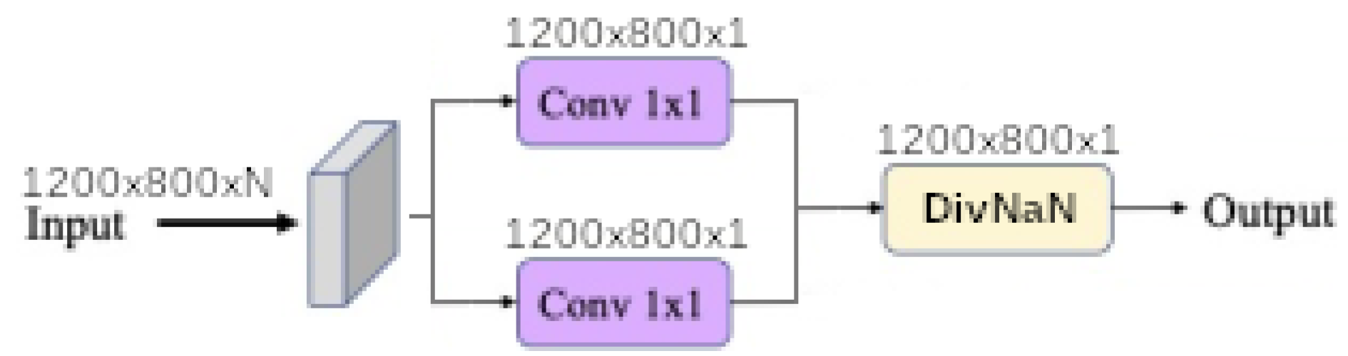
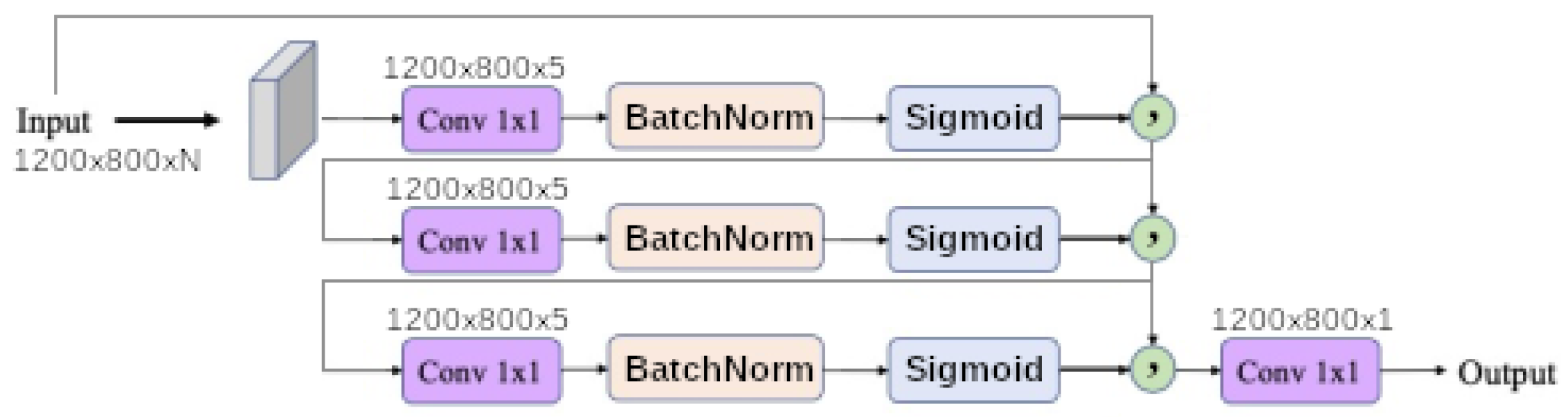
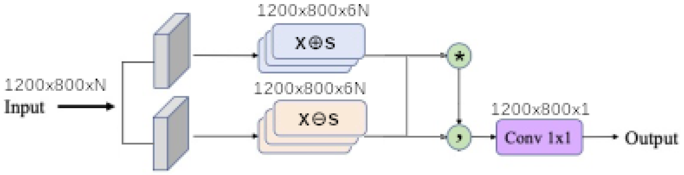
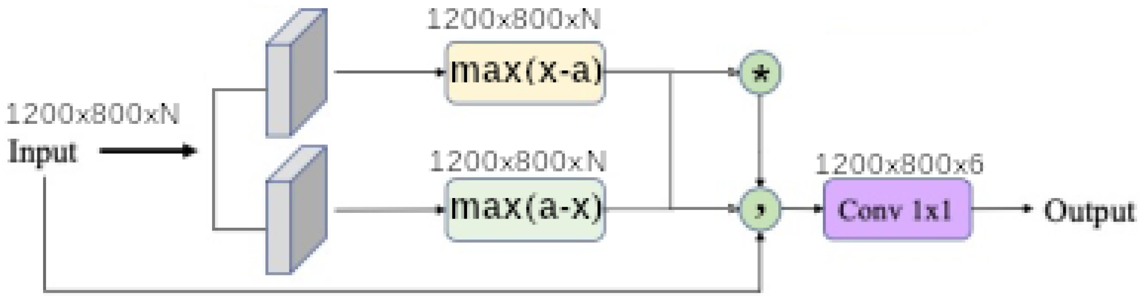
Finally, each baseline model such as linear, linear ratio, polynomial, universal function approximation and dense morphological function approximation are evaluated with 4 different modalities of each kernel size N = 1 , N = 3 , N = 5 and N = 7 . In addition 
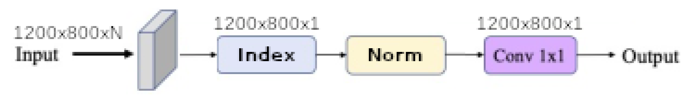
input band filter (ibf) and spatial pyramid refinement block (sprb) are put respectively at the upstream and downstream of the network. 
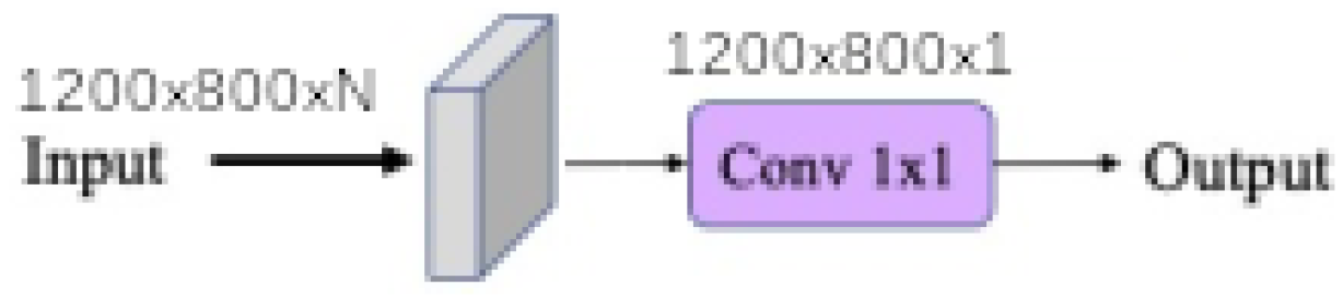
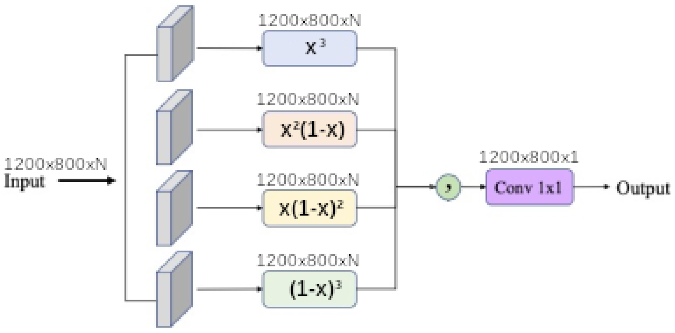
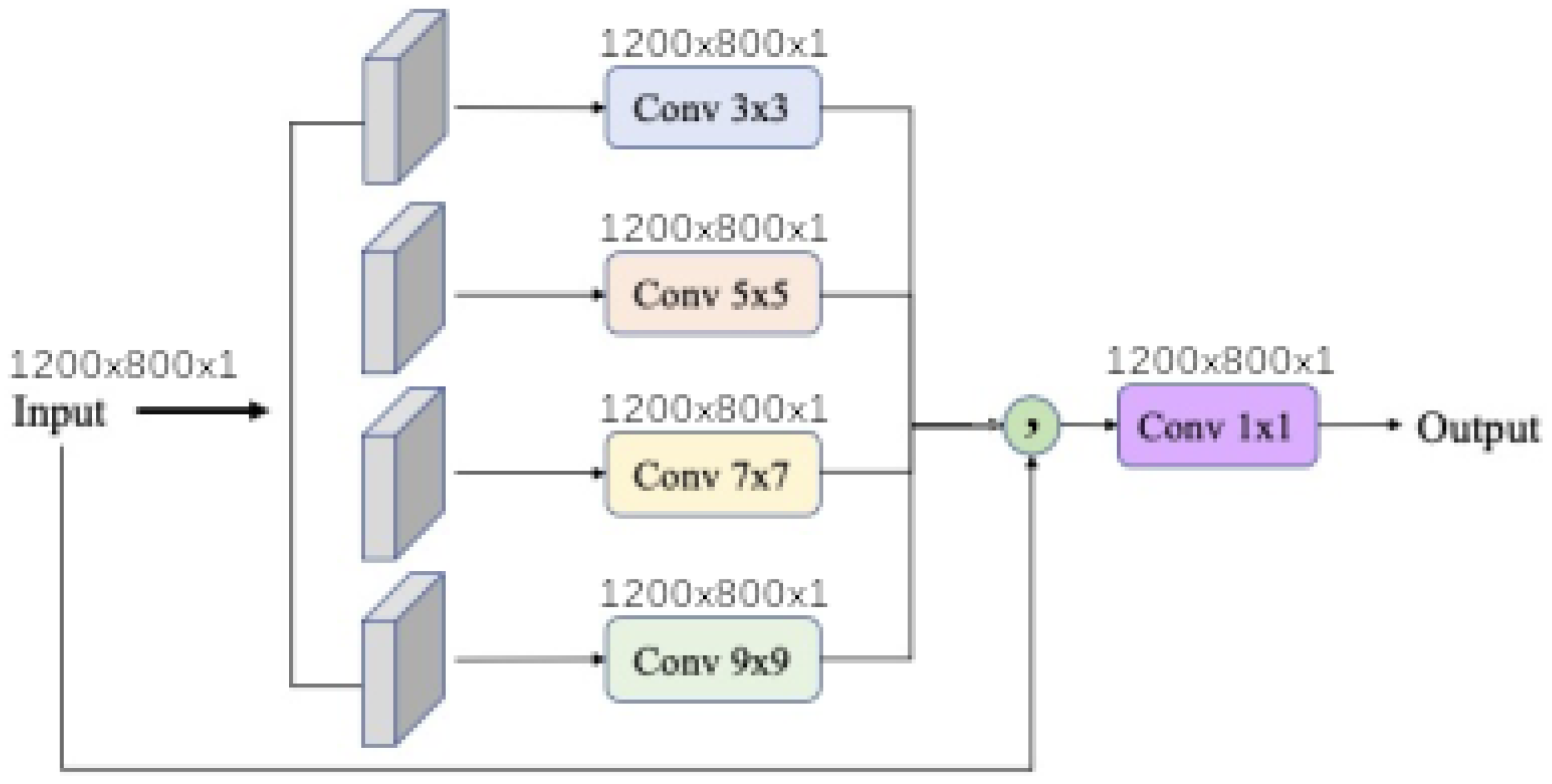
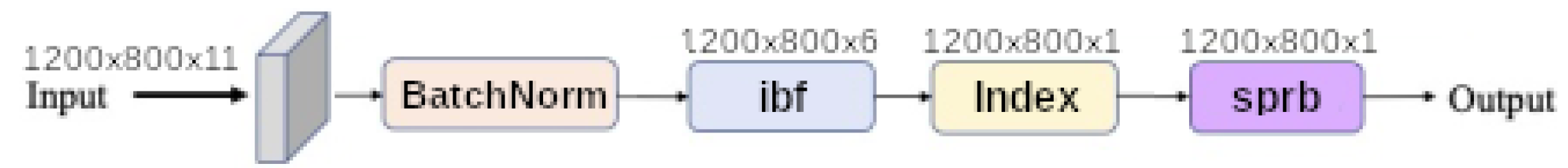
Figure 11 shows that network synthesis. To deal with lighting variation and saturation a BatchNormalization is put in the upstream of the network in all cases. The ibf and sprb modules are optional and can be disabled.
When the input band filter (ibf) is enabled, the incoming tensor size of 1200 × 800 × 13 is transformed to a tensor of size 1200 × 800 × 6 and passed to the generic equation. When it is not, the generic equations get the raw input tensor of size 1200 × 800 × 13 . In all cases the baseline model output a tensor of shape 1200 × 800 × 1 . The spatial pyramid refinement block transforms the output tensor of the baseline model to a new tensor of the same size.
All models are evaluated with two metrics, respectively the dice and mIoU score. For each kernel size, the results are presented in Table 3, Table 4, Table 5 and Table 6. All models are also evaluated with and without ibf and sprb for each kernel size.
For all baseline models, the results (in term of mIoU) show that increasing the kernel size also increases performances. The gain performance between best models in kernel size 1 and 7 are approximately 2 % and then correspond to the influence of spectral mixing. So searching for spectral mixing 3 pixels farther (kernel size 7) still increases performance. It could also be possible that function approximation allows to spatially reconstruct some missing information.
For all kernel sizes, the ibf module enhance the mIoU score up to 3.6 % . So the ibf greatly prune the unneeded part of the input signal which increases the separability and the performances of all models. The sprb module allows to smooth the output by taking into account neighborhood indices, but their performance are not always better or generally negligible when it is used alone with the baseline model.
The baseline polynomial model is probably over-fitted, because it’s hard to find the good polynomial order. But enabling the ibf fixes this issue. However further study should be done to setup the order of Bernstein expansion.
The dense morphological with a kernel size of 5 and 7 using both ibf and sprb modules is the best model in term of dice (≈ 90 % ) and mIoU score (≈ 82 % ). Followed by universal function approximator with a kernel size of 1 or 3 with both ibf and sprb modules (dice up to 89 % and mIoU up to 81 % ). Further studies on the width of the universal function approximator could probably increase performance. According to [43] it seems normal that the potential of dense morphological is higher although the hyper-parameters optimization of universal function approximator could increase their performance.

4.3. Initial Image Processing

To show the importance of the initial image processing, each model has been trained without the various input transformations, such as ρ s t d , Gxx, Gxy, Gyy filters, Laplacian filter, minimum and maximum Eigen values. Table 7 shows the score of DeepIndices considering only kernel size of 1 in different model.
The results shows that none of optimized models outperforms the previous performance with the initial image processing (best mIoU at 80.15 % ). The maximum benefit is approximately 6 % for mIoU score depending on the model and module, especially when using combination of ibf, sprb and small kernel size. Meaning that signal processing is much more important than spectral mixing and texture.

4.4. Discussion

Further improvements can be set on hyper-parameters of the previously defined equations, such as the degree of the polynomial (set to 11), the CNN depth and width for Taylor series (set to 3) and the number of operations in morphological network (set to 10). In particular the learning of 2D convolution kernel of Taylor series may be replaced by a structured receptive field [41]. In addition it would be interesting to transpose our study with new data for other surfaces such as shadows, waters, clouds or snows.
The training dataset is randomly split with a fixed seed, which is used for every learned models. As previously noted, this is important to ensure reproducible results but could also favor specific models. Further work to evaluate the impact of varying training datasets could be conducted.

4.4.1. Model Convergence

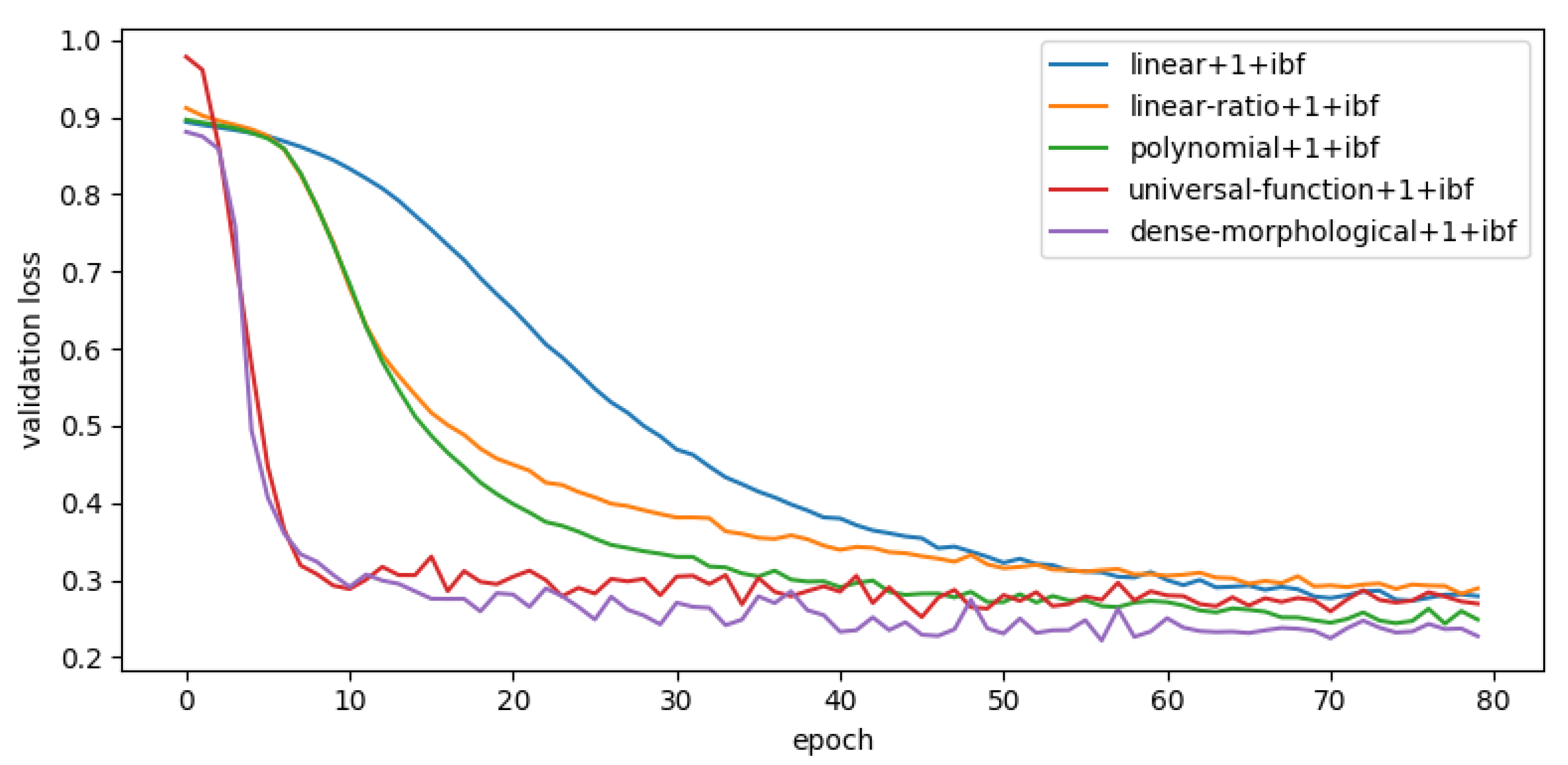
Another way to estimate the robustness of a model against its initialization is to compare the model’s convergence speed. Models with faster convergence should be less sensitive to the training dataset. As an example, the convergence speed of few different models is shown in Figure 12. The baseline model convergence is the same, as well as sprb module. However the speed of convergence also increases with the size of the kernel but does not alter subsequent observations. For greater readability only models with ibf are presented.
An important difference in the speed of convergence between models is observed. An analysis of this figure allows the aggregation of model types and speed:
  • Slow converging models: polynomials models converge slowly as well as the majority of linear or linear-ratio models.
  • Fast converging models: universal-functions and dense-morphological are the fastest to converge (less than 30 iterations)
A subset of slow and fast converging models could be evaluated in term of sensitivity against initialization. It shows that the dense morphological followed by universal function approximator convergence faster than the other. Regardless of the used module nor kernel size.

4.4.2. Limits of Deepindices

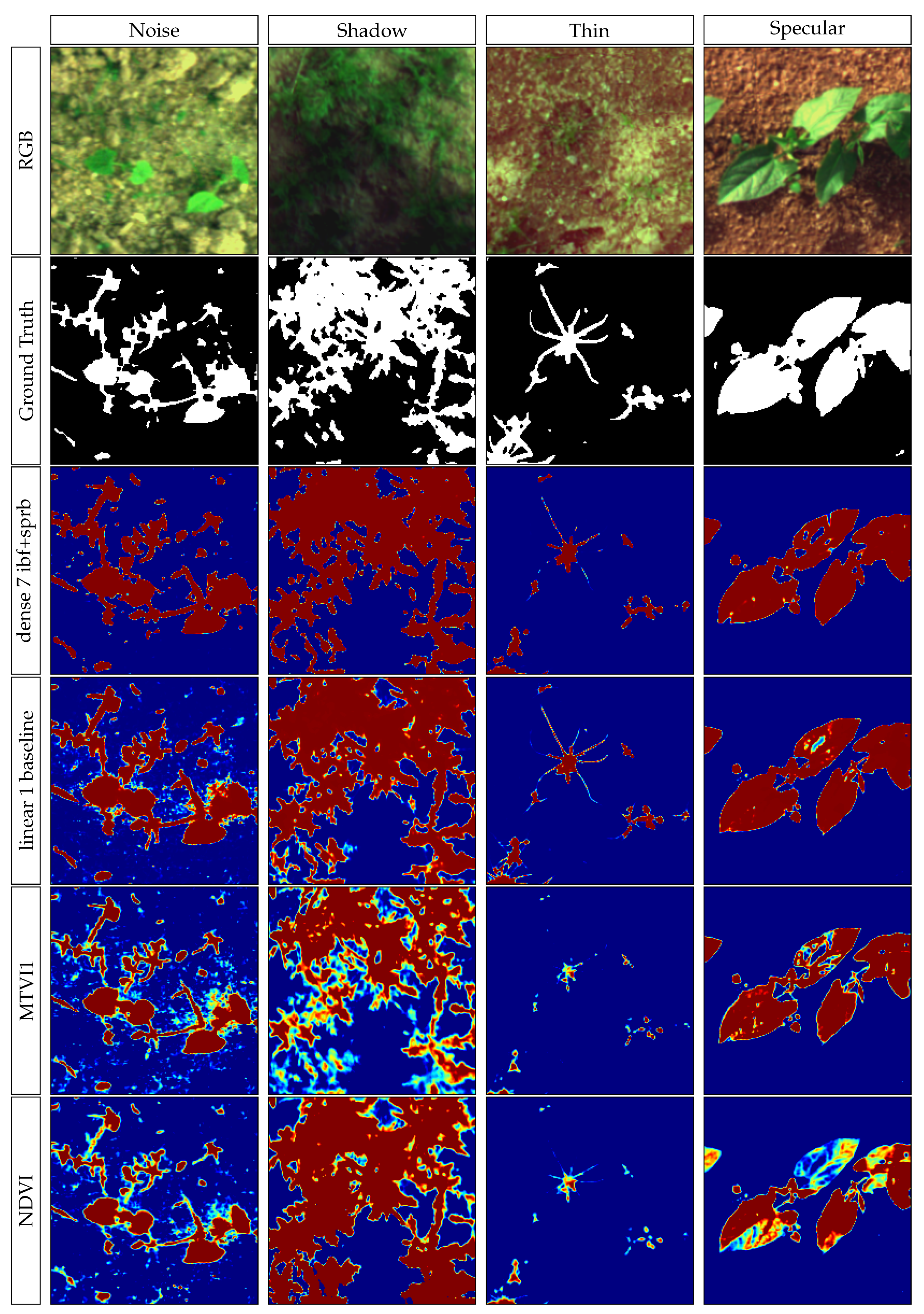
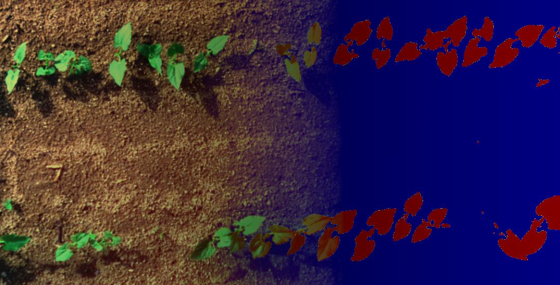
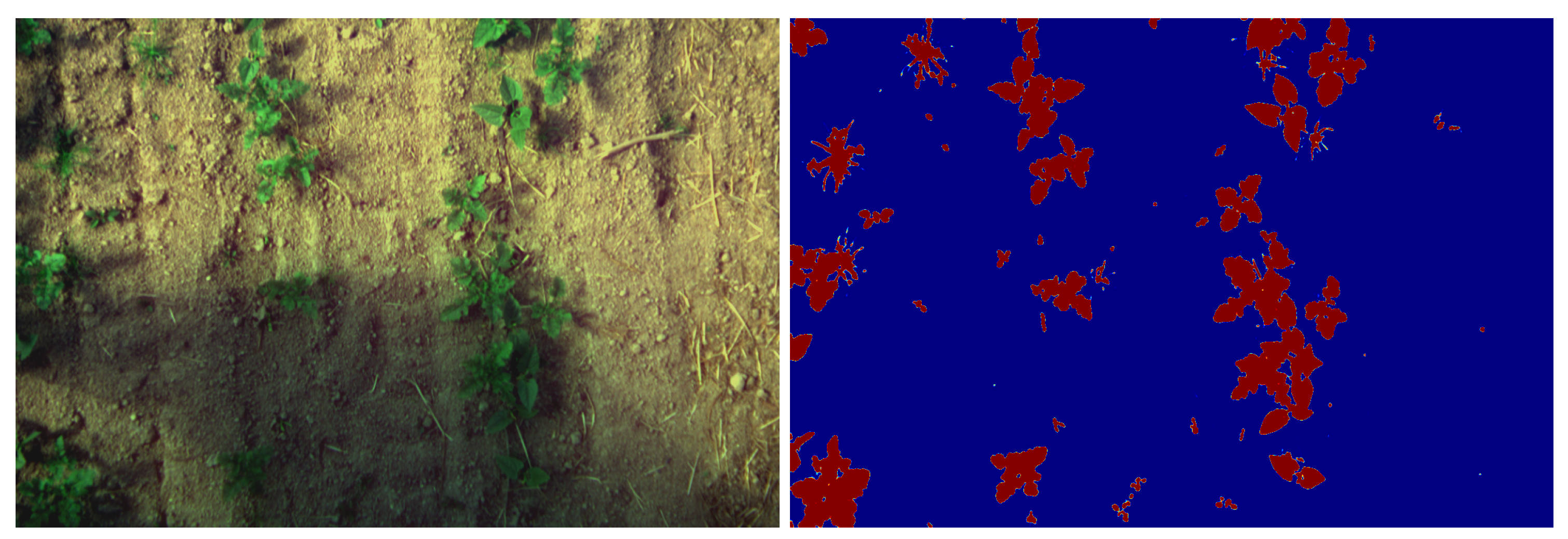
Shadows can be a relatively hard problem to solve in image processing, the proposed models are able to correctly separate vegetation from soil even with shadowy images, as shown in Figure 13. In addition, the Figure A1 in the Appendix A shows the impacts of various acquisition factors, such as shadow, noise, specular or thin vegetation features.
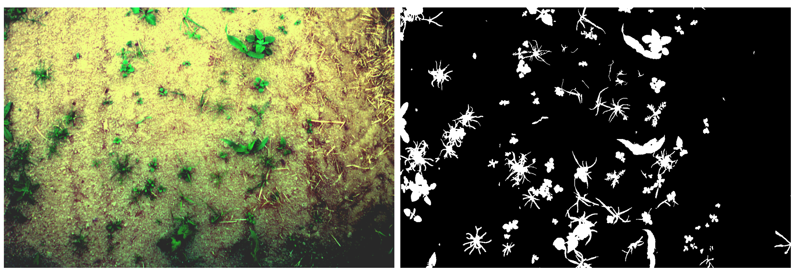
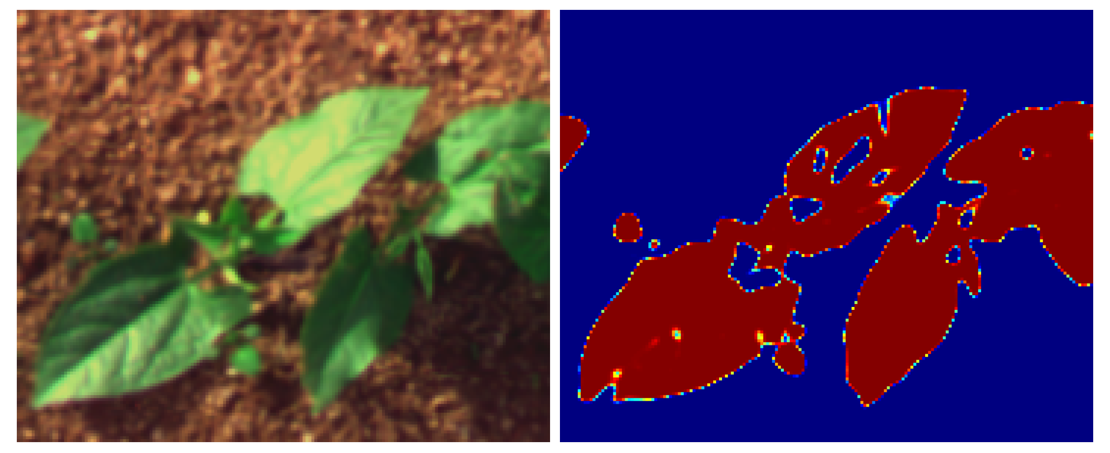
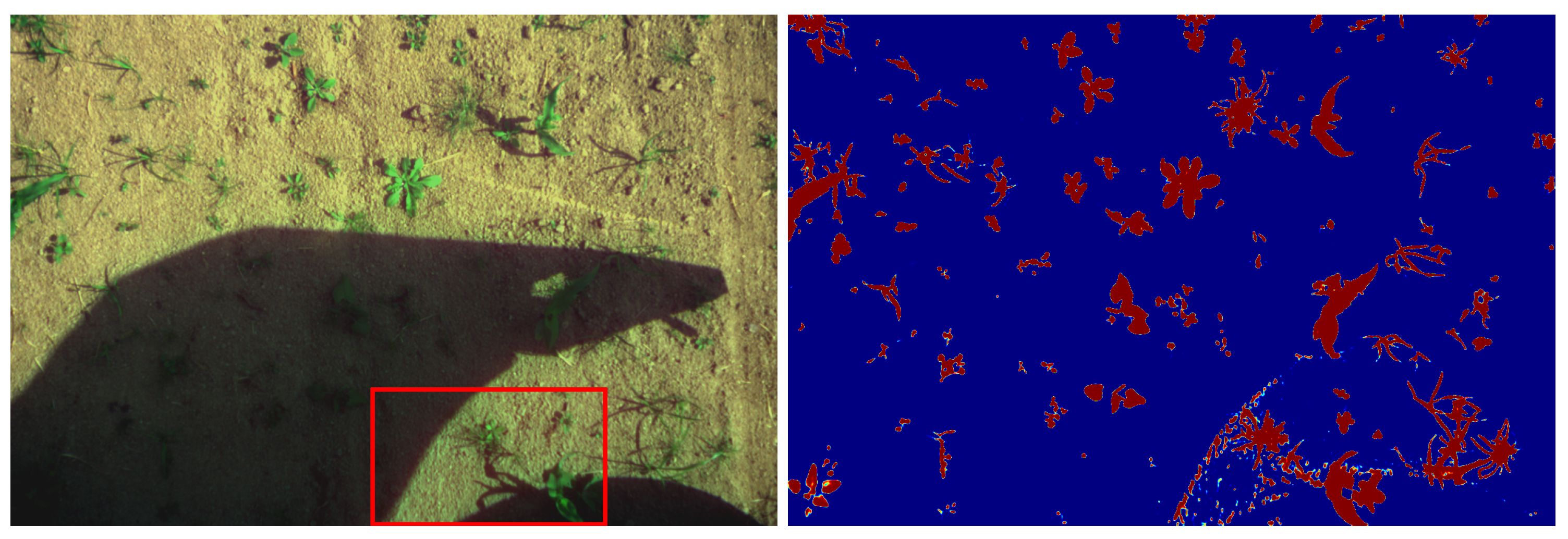
Some problem occurs when there are abrupt transitions between shadowed and light areas of an image as shown in Figure 14.
It appears that the discrimination error appears where the shadow is cast by a solid object, resulting in edge diffraction that creates small fringes on the soil and vegetation. A lack of such images in the training dataset could explain the model failure. Data augmentation could be used to obtain a training model containing such images, from cloud shadows to solid objects shadows. Further work is needed to estimate the benefit of such a data augmentation on the developed models.
The smallest parts of the vegetation (less than 1 pixel, such as small monocotyledon leaves or plant stems) cannot be detected because of a strong spectral mixture. This limitation is due to the acquisition conditions (optics, CCD resolution and elevation) and should be considered as is. As vegetation with a width over 1 pixel is correctly segmented by our approach, the acquisition parameters should be chosen so that the smallest parts of vegetation that are required by an application are larger than 1 pixel in the resulting image.
A few spots of specular light can also be observed on images, particularly on leaves. These spots are often unclassified (or classified as soil). This modifies the shape of the leaves by creating holes inside them. This problem can be seen on Figure 15. Leaves with holes are visible on the left and the middle of the top bean row. It would be interesting to train the network to detect and assign them to a dedicated class.
Next the location of the detected spots could be studied to re-assign them to two classes: specular-soil and specular-vegetation. To perform this step, a semantic segmentation could be set up to identify the surrounding objects of the holes specifically. It would be based on the UNet model, which performs a multi-scale approach by calculating, treating and re-convolving images of lower resolutions.
More generally, the quality of the segmentation between soil and vegetation strongly influences the discrimination between crop and weed, which remains a major application following this segmentation task. Three categories of troubles have been identified: the plants size, the ambient light variations (shades, specular light spots), and the morphological complexity of the studied objects.
The size of the plants mainly impacts their visibility on the acquired images. It is not obviously related to the ability of the algorithm to classify them. However, it leads to the absence of essential elements such as monocotyledon weeds at an early vegetation stage. A solution is proposed by setting the acquisition conditions to let the smallest vegetation part be over 1 pixel.
Conversely, the variations of ambient light should be treated by the classification algorithm. As previously mentioned, shadow management needs an improvement of the learning base, and specular light spots could be treated by a multi-scale approach. Their influence on the discrimination step should be major. Indeed, they influence the shape of the objects classified as plants, which is a useful criterion to discriminate crops from weeds. The morphological complexity of the plants can be illustrated by the presence of stems. In our case, bean stems are similar to weed leaves. This problem should be treated by the discrimination step. The creation of a stem class (in addition to the weed and crop classes) will be studied in particular.

5. Conclusions

In this work, different standard vegetation indices have been evaluated as well as different methods to estimate new DeepIndices through different types of equations that can reconstruct the others. Among the 89 standard vegetation indices tested, the MTVI (Modified Triangular Vegetation Index 1) gives the best vegetation segmentation. Standard indices remain sub-optimal even if they are downstream optimized with a linear regression because they are usually used on calibrated reflectance data. The results allow us to conclude that any simple linear combination is just more efficient ( + 4.87 % mIoU) than any standard indices by taking into account all spectral bands and few transformations. The results also suggest that un-calibrated data can be used in proximal sensing applications for both standard indices and DeepIndices with good performances.
We therefore agree that it is important to optimize both the arithmetic structure of the equation and the coefficients of the spectral bands, that is why our automatically generated indices are much more accurate. The best model is much more efficient by + 8.48 % compared to the best standard indices and by + 18.21 % compared to NDVI. Also the two modules ibf, sprb and the initial image transformation show a significant improvement. The developed DeepIndices allow to take into account the lighting variation within the equation. It makes possible to abstract from a difficult problem which is the data calibration. Thus, partially shaded images are correctly evaluated, which is not possible with standard indices since they use sprectum measurement that change with shades. However, it would be interesting to evaluate the performance of standard indices and DeepIndices on calibrated reflectance data.
These results suggest that deep learning algorithms are a useful tool to discover the spectral band combinations that identify the vegetation in multi spectral camera. Another conclusion from this research is about the genericity of the methodology developed. This study presents a first experiment employed in field images with the objective of finding deep vegetation indices and demonstrates their effectiveness compared to standard vegetation indices. This paper’s contribution improves the classical methods of vegetation index development and allows the generation of more precise indices (i.e., DeepIndices). The same kind of conclusion may arise from this methodology applied on remote sensing indices to discriminates other surfaces (roads, water, snow, shadows, etc).

Author Contributions

Conceptualization, J.-A.V.; data curation, J.-A.V.; formal analysis, J.-A.V.; funding acquisition, G.J. and J.-N.P.; investigation, J.-A.V.; methodology, J.-A.V.; project administration, Paoli.J-N. and G.J.; resources, Paoli.J-N. and G.J.; software, J.-A.V.; supervision, J.-N.P. and G.J.; validation, J.-N.P.; C.G. and G.J.; visualization, J.-A.V.; writing—original draft preparation, J.-A.V.; writing—review and editing, J.-A.V.; J.-N.P.; C.G. and G.J. All authors have read and agreed to the published version of the manuscript.

Funding

This project is funded by ANR Challenge RoSE and the Horizon 2020 project IWMPRAISE.

Institutional Review Board Statement

Not applicable.

Informed Consent Statement

Not applicable: this studies did not involve humans or animals.

Data Availability Statement

Data in this study is publicly available at https://data.inrae.fr/dataset.xhtml?persistentId=doi:10.15454/DSQC8N, using Creative Common CC0 1.0 Public Domain Dedication licence.

Acknowledgments

We would like to thank Masson Jean-Benoit for the realization of the metal gantry which allowed us to position the camera at different heights, it was used in particular for the calibration of the camera and the band registration. We also thank Djemai Mehdi for the spelling correction of the English. And we thank Aubry Clément and Cozic Thibault of the company SITIA for their help in interfacing the camera with the used robot “Trecktor”.

Conflicts of Interest

The authors declare no conflict of interest. The funders had no role in the design of the study; in the collection, analyses, or interpretation of data; in the writing of the manuscript, or in the decision to publish the results.

Appendix A

Table A1. Top optimized fixed vegetation model equations. b = ρ 0 , g = ρ 1 , r = ρ 2 , e = ρ 3 , u = ρ 4 , n = ρ 5 .
ModelEquation
Modified Triangular Vegetation Index 1 1.2 ( 1.2 ( n g ) 2.5 ( r g ) )
Modified Chlorophyll Absorption In Reflectance Index 1 1.2 ( 2.5 ( n r ) 1.3 ( n g ) )
Enhanced Vegetation Index 2 2.4 ( n r ) / ( n + r + 1 )
Soil Adjusted Vegetation Index 2.0 ( n r ) / ( n + r + 1.0 )
Soil And Atmospherically Resistant VI 3 1.5 ( n r ) / ( n + r + 0.5 )
Enhanced Vegetation Index 3 2.5 ( n r ) / ( n + 2.4 r + 1 )
Global Environment Monitoring Index 2 ( n 2 r 2 ) + 1.5 n + 0.5 r n + r + 0.5 ( 1 n / 4 ) r 0.125 1 + r
Adjusted Transformed Soil Adjusted VI a n a r 0.03 a n + r a 0.03 + 0.08 ( 1 + a 2 ) a = 1.22
NDVI ( n r ) / ( n + r )
Figure A1. Visual comparison between some relevant models. NDVI (63.98 mIoU), MTVI1 (73.71 mIoU), linear 1 baseline (78.58 mIoU), dense 7 ibf-sprb (82.19 mIoU). Blue indicates sure soil, red indicates sure vegetation, and the other colors indicate uncertainty.
Remotesensing 13 02261 g0a1

References

  1. Jinru, X.; Su, B. Significant Remote Sensing Vegetation Indices: A Review of Developments and Applications. J. Sens. 2017, 2017, 1353691. [Google Scholar] [CrossRef] [Green Version]
  2. Jiří, M.; Lukas, V.; Elbl, J.; Smutny, V. Comparison of Sentinel–2 and ISARIA winter wheat mapping for variable rate application of nitrogen fertilizers. In Proceedings of the MendelNet 2019: Proceedings of International PhD Students Conference, Brno, Czech Republic, 6–7 November 2019. [Google Scholar]
  3. Tanrıverdi, C.; Fakültesi, Z.; Yapılar, T.; Bölümü, S.; Kahramanmaraş; Tarımda, H.; Algılama, U.; İndekslerinin, B.; Derlemesi, B. A Review of Remote Sensing and Vegetation Indices in Precision Farming. J. Sci. Eng 2006, 9, 69–76. [Google Scholar]
  4. Elbeltagi, A.; Kumari, N.; Dharpure, J.K.; Mokhtar, A.; Alsafadi, K.; Kumar, M.; Mehdinejadiani, B.; Ramezani Etedali, H.; Brouziyne, Y.; Towfiqul Islam, A.R.M.; et al. Prediction of Combined Terrestrial Evapotranspiration Index (CTEI) over Large River Basin Based on Machine Learning Approaches. Water 2021, 13, 547. [Google Scholar] [CrossRef]
  5. Lee, M.K.; Golzarian, M.; Kim, I. A new color index for vegetation segmentation and classification. Precis. Agric. 2020, 22, 179–204. [Google Scholar] [CrossRef]
  6. Milioto, A.; Lottes, P.; Stachniss, C. Real-time Semantic Segmentation of Crop and Weed for Precision Agriculture Robots Leveraging Background Knowledge in CNNs. arXiv 2017, arXiv:1709.06764. [Google Scholar]
  7. Hassanein, M.; Lari, Z.; El-Sheimy, N. A New Vegetation Segmentation Approach for Cropped Fields Based on Threshold Detection from Hue Histograms. Sensors 2018, 18, 1253. [Google Scholar] [CrossRef] [Green Version]
  8. Dixit, A.; Goswami, A.; Jain, S. Development and Evaluation of a New “Snow Water Index (SWI)” for Accurate Snow Cover Delineation. Remote Sens. 2019, 11, 2774. [Google Scholar] [CrossRef] [Green Version]
  9. Zhai, H.; Zhang, H.; Zhang, L.; Li, P. Cloud/shadow detection based on spectral indices for multi/hyperspectral optical remote sensing imagery. ISPRS J. Photogramm. Remote Sens. 2018, 144, 235–253. [Google Scholar] [CrossRef]
  10. Henrich, V.; Götze, E.; Jung, A.; Sandow, C.; Thürkow, D.; Gläßer, C. Development of an online indices database: Motivation, concept and implementation. In Proceedings of the 6th EARSeL Imaging Spectroscopy SIG Workshop Innovative Tool for Scientific and Commercial Environment Applications, Tel Aviv, Israel, 16–18 March 2009; pp. 16–18. [Google Scholar]
  11. Zhang, L.; Sun, X.; Wu, T.; Zhang, H. An Analysis of Shadow Effects on Spectral Vegetation Indexes Using a Ground-Based Imaging Spectrometer. IEEE Geosci. Remote Sens. Lett. 2015, 12, 2188–2192. [Google Scholar] [CrossRef]
  12. Gitelson, A.A. Wide dynamic range vegetation index for remote quantification of biophysical characteristics of vegetation. J. Plant Physiol. 2004, 161, 165–173. [Google Scholar] [CrossRef] [Green Version]
  13. Liu, P.; Shi, R.; Zhang, C.; Zeng, Y.; Wang, J.; Tao, Z.; Gao, W. Integrating multiple vegetation indices via an artificial neural network model for estimating the leaf chlorophyll content of Spartina alterniflora under interspecies competition. Environ. Monit. Assess. 2017, 189. [Google Scholar] [CrossRef]
  14. Kokhan, S.; Vostokov, A. Using Vegetative Indices to Quantify Agricultural Crop Characteristics. J. Ecol. Eng. 2020, 21, 120–127. [Google Scholar] [CrossRef]
  15. Yahui, G.; Senthilnath, J.; Wu, W.; Zhang, X.; Zeng, Z.; Huang, H. Radiometric Calibration for Multispectral Camera of Different Imaging Conditions Mounted on a UAV Platform. Sustainability 2019, 11, 978. [Google Scholar] [CrossRef] [Green Version]
  16. Minařík, R.; Langhammer, J.; Hanuš, J. Radiometric and Atmospheric Corrections of Multispectral MCA Camera for UAV Spectroscopy. Remote Sens. 2019, 11, 2428. [Google Scholar] [CrossRef] [Green Version]
  17. Gilliot, J.M.; Michelin, J.; Faroux, R.; Domenzain, L.M.; Fallet, C. Correction of in-flight luminosity variations in multispectral UAS images, using a luminosity sensor and camera pair for improved biomass estimation in precision agriculture. In Proceedings of the 2018 Autonomous Air and Ground Sensing Systems for Agricultural Optimization and Phenotyping III, Bellingham, WA, USA, 16–17 April 2018. [Google Scholar] [CrossRef]
  18. Chebrolu, N.; Lottes, P.; Schaefer, A.; Winterhalter, W.; Burgard, W.; Stachniss, C. Agricultural robot dataset for plant classification, localization and mapping on sugar beet fields. Int. J. Robot. Res. 2017, 36. [Google Scholar] [CrossRef] [Green Version]
  19. Wu, X.; Aravecchia, S.; Pradalier, C. Design and Implementation of Computer Vision based In-Row Weeding System. In Proceedings of the 2019 International Conference on Robotics and Automation (ICRA), Montreal, QC, Canada, 20–24 May 2019; pp. 4218–4224. [Google Scholar] [CrossRef] [Green Version]
  20. Oldeland, J.; Dorigo, W.; Lieckfeld, L.; Lucieer, A.; Jürgens, N. Combining vegetation indices, constrained ordination and fuzzy classification for mapping semi-natural vegetation units from hyperspectral imagery. Remote Sens. Environ. 2010, 114, 1155–1166. [Google Scholar] [CrossRef]
  21. Peña-Barragán, J.M.; Ngugi, M.K.; Plant, R.E.; Six, J. Object-based crop identification using multiple vegetation indices, textural features and crop phenology. Remote Sens. Environ. 2011, 115, 1301–1316. [Google Scholar] [CrossRef]
  22. Nguy-Robertson, A.; Gitelson, A.; Peng, Y.; Viña, A.; Arkebauer, T.; Rundquist, D. Green leaf area index estimation in maize and soybean: Combining vegetation indices to achieve maximal sensitivity. Agron. J. 2012, 104, 1336–1347. [Google Scholar] [CrossRef] [Green Version]
  23. Shishir, S.; Tsuyuzaki, S. Hierarchical classification of land use types using multiple vegetation indices to measure the effects of urbanization. Environ. Monit. Assess. 2018, 190. [Google Scholar] [CrossRef]
  24. Lu, J.; Cheng, D.; Geng, C.; Zhang, Z.; Xiang, Y.; Hu, T. Combining plant height, canopy coverage and vegetation index from UAV-based RGB images to estimate leaf nitrogen concentration of summer maize. Biosyst. Eng. 2021, 202, 42–54. [Google Scholar] [CrossRef]
  25. Kabiri, P.; Pandi, M.; Nejat, S. NDVI Optimization Using Genetic Algorithm. In Proceedings of the IEEE 2011 7th Iranian Conference on Machine Vision and Image Processing, Tehran, Iran, 16–17 November 2011; pp. 1–5. [Google Scholar] [CrossRef]
  26. Albarracín, J.; Oliveira, R.; Hirota, M.; Santos, J.; Torres, R. A Soft Computing Approach for Selecting and Combining Spectral Bands. Remote Sens. 2020, 12, 2267. [Google Scholar] [CrossRef]
  27. Lv, X.; Ming, D.; Lu, T.; Zhou, K.; Wang, M.; Bao, H. A New Method for Region-Based Majority Voting CNNs for Very High Resolution Image Classification. Remote Sens. 2018, 10, 1946. [Google Scholar] [CrossRef] [Green Version]
  28. Gaetano, R.; Ienco, D.; Ose, K.; Cresson, R. A Two-Branch CNN Architecture for Land Cover Classification of PAN and MS Imagery. Remote Sens. 2018, 10, 1746. [Google Scholar] [CrossRef] [Green Version]
  29. Fu, T.; Ma, L.; Li, M.; Johnson, B.A. Using convolutional neural network to identify irregular segmentation objects from very high-resolution remote sensing imagery. J. Appl. Remote Sens. 2018, 12, 025010. [Google Scholar] [CrossRef]
  30. Kussul, N.; Lavreniuk, M.; Skakun, S.; Shelestov, A. Deep Learning Classification of Land Cover and Crop Types Using Remote Sensing Data. IEEE Geosci. Remote Sens. Lett. 2017, 14, 778–782. [Google Scholar] [CrossRef]
  31. Bajwa, S.; Tian, L. Multispectral CIR image calibration for cloud shadow and soil background influence using intensity normalization. Appl. Eng. Agric. 2002, 18, 627–635. [Google Scholar] [CrossRef]
  32. Bareth, G.; Bolten, A.; Gnyp, M.L.; Reusch, S.; Jasper, J. Comparison of Uncalibrated Rgbvi with Spectrometer-Based Ndvi Derived from Uav Sensing Systems on Field Scale. ISPRS Int. Arch. Photogramm. Remote. Sens. Spat. Inf. Sci. 2016, 41B8, 837–843. [Google Scholar] [CrossRef]
  33. Louargant, M.; Villette, S.; Jones, G.; Vigneau, N.; Paoli, J.; Gée, C. Weed detection by UAV: Simulation of the impact of spectral mixing in multispectral images. Precis. D 2017, 932–951. [Google Scholar] [CrossRef] [Green Version]
  34. Vayssade, J.A.; Jones, G.; Paoli, J.N.; Gée, C. Two-step multi-spectral registration via key-point detector and gradient similarity. Application to agronomic scenes for proxy-sensing. In Proceedings of the 15th International Joint Conference on Computer Vision, Imaging and Computer Graphics Theory and Applications, Valletta, Malta, 27–29 February 2020. [Google Scholar]
  35. Khanna, R.; Sa, I.; Nieto, J.; Siegwart, R. On field radiometric calibration for multispectral cameras. In Proceedings of the 2017 IEEE International Conference on Robotics and Automation (ICRA), Singapore, 29 May–3 June 2017; pp. 6503–6509. [Google Scholar] [CrossRef]
  36. Blackburn, G.; Vignola, F. Spectral distributions of diffuse and global irradiance for clear and cloudy periods. In Proceedings of the World Renewable Energy Forum, Denver, CO, USA, 19–21 January 2012. [Google Scholar]
  37. Lin, B.; Sun, Y.; Sanchez, J. Efficient Vessel Feature Detection for Endoscopic Image Analysis. IEEE Trans. Biomed. Eng. 2014, 62, 1141–1150. [Google Scholar] [CrossRef]
  38. Jang, S.; Son, Y. Empirical Evaluation of Activation Functions and Kernel Initializers on Deep Reinforcement Learning. In Proceedings of the 2019 International Conference on Information and Communication Technology Convergence (ICTC), Jeju Island, Korea, 16–18 October 2019; pp. 1140–1142. [Google Scholar]
  39. Sun, H.; Hou, M.; Yang, Y.; Zhang, T.; Weng, F.; Han, F. Solving Partial Differential Equation Based on Bernstein Neural Network and Extreme Learning Machine Algorithm. Neural Process. Lett. 2019, 50, 1153–1172. [Google Scholar] [CrossRef]
  40. Geusebroek, J.M.; van den Boomgaard, R.; Smeulders, A.; Dev, A. Color and Scale: The Spatial Structure of Color Images. In Proceedings of the European Conference on Computer Vision, Glasgow, UK, 23–28 August 2000; pp. 331–341. [Google Scholar] [CrossRef]
  41. Jacobsen, J.H.; Gemert, J.; Lou, Z.; Smeulders, A. In Proceedings of the IEEE Conference on Computer Vision and Pattern Recognition Structured Receptive Fields in CNNs, Las Vegas, NV, USA, 26 June–1 July 2016; pp. 2610–2619. [CrossRef] [Green Version]
  42. Huang, G.; Liu, Z.; Weinberger, K.Q. Densely Connected Convolutional Networks. arXiv 2016, arXiv:1608.06993. [Google Scholar]
  43. Mondal, R.; Santra, S.; Chanda, B. Dense Morphological Network: An Universal Function Approximator. arXiv 2019, arXiv:1901.00109. [Google Scholar]
  44. Joshi, E.; Sasode, D.S.; Singh, N.; Chouhan, N. Revolution of Indian Agriculture through Drone Technology. Biot. Res. Today 2020, 2, 174–176. [Google Scholar]
  45. Liu, W.; Rabinovich, A.; Berg, A.C. ParseNet: Looking Wider to See Better. arXiv 2015, arXiv:1506.04579. [Google Scholar]
  46. Bokhovkin, A.; Burnaev, E. Boundary Loss for Remote Sensing Imagery Semantic Segmentation. arXiv 2019, arXiv:1905.07852. [Google Scholar]
  47. Rahman, M.; Wang, Y. Optimizing Intersection-Over-Union in Deep Neural Networks for Image Segmentation. In Proceedings of the International Symposium on Visual Computing, San Diego, CA, USA, 5–7 October 2016; Volume 10072, pp. 234–244. [Google Scholar] [CrossRef]
  48. Zhou, D.; Fang, J.; Song, X.; Guan, C.; Yin, J.; Dai, Y.; Yang, R. IoU Loss for 2D/3D Object Detection. arXiv 2019, arXiv:1908.03851. [Google Scholar]
  49. van Beers, F.; Lindström, A.; Okafor, E.; Wiering, M.A. Deep Neural Networks with Intersection over Union Loss for Binary Image Segmentation. In Proceedings of the ICPRAM, Prague, Czech Republic, 19–21 February 2019; pp. 438–445. [Google Scholar]
  50. Jadon, S. A survey of loss functions for semantic segmentation. In Proceedings of the 2020 IEEE Conference on Computational Intelligence in Bioinformatics and Computational Biology (CIBCB), Viña del Mar, Chile, 27–29 October 2020; pp. 1–7. [Google Scholar]
  51. Aggarwal, R.; Ranganathan, P. Common pitfalls in statistical analysis: The use of correlation techniques. Perspect. Clin. Res. 2016, 7, 187. [Google Scholar] [CrossRef]
  52. Armstrong, R.A. Should Pearson’s correlation coefficient be avoided? Ophthalmic Physiol. Opt. 2019, 39, 316–327. [Google Scholar] [CrossRef] [Green Version]
  53. Shamir, R.R.; Duchin, Y.; Kim, J.; Sapiro, G.; Harel, N. Continuous Dice Coefficient: A Method for Evaluating Probabilistic Segmentations. arXiv 2019, arXiv:1906.11031. [Google Scholar]
  54. Choi, H.; Lee, H.J.; You, H.J.; Rhee, S.Y.; Jeon, W.S. Comparative Analysis of Generalized Intersection over Union and Error Matrix for Vegetation Cover Classification Assessment. Sens. Mater. 2019, 31, 3849. [Google Scholar] [CrossRef]
  55. Zhang, M.R.; Lucas, J.; Hinton, G.E.; Ba, J. Lookahead Optimizer: K steps forward, 1 step back. arXiv 2019, arXiv:1907.08610. [Google Scholar]
Figure 1. AIRPHEN camera composed of 6 sensors.
Remotesensing 13 02261 g001
Figure 2. False color in the left and corresponding manual ground truth on the right.
Remotesensing 13 02261 g002
Figure 3. Linear combination model.
Remotesensing 13 02261 g003
Figure 4. Linear ratio model.
Remotesensing 13 02261 g004
Figure 5. Polynomial model with Bernstein expansions between B 4 , 1 and B 4 , 4 .
Remotesensing 13 02261 g005
Figure 6. Universal function approximation model (depth = 3, width = 5).
Remotesensing 13 02261 g006
Figure 7. Dense-morphological model.
Remotesensing 13 02261 g007
Figure 8. Input Band Filter inserted at the beginning of the model.
Remotesensing 13 02261 g008
Figure 9. Spatial refinement block inserted at the end of a model.
Remotesensing 13 02261 g009
Figure 10. Optimized model for standard indices.
Remotesensing 13 02261 g010
Figure 11. Network synthesis with ibf, evalated index equation, and sprb.
Remotesensing 13 02261 g011
Figure 12. First 80 epochs of loss of generic models with ibf in kernel size of 1.
Remotesensing 13 02261 g012
Figure 13. Correct vegetation/soil discrimination despite shadows.
Remotesensing 13 02261 g013
Figure 14. Vegetation/soil discrimination issue with abrupt transition between shadow and light.
Remotesensing 13 02261 g014
Figure 15. Vegetation/soil discrimination issue caused by specular lights on leaves.
Remotesensing 13 02261 g015
Table 1. Acquisition sources and global illumination.
SourceYearCornBeanIllumination
Dijon2019-9full sun, evening
Montoldre20192022shadow, sunny, cloudy
Montoldre20201822morning, cloudy, rainy
total 3853=91
Table 2. Synthesized standard indices performances: the nine best models are presented.
Standard IndexUsed ρ mIoUDice
Modified Triangular Vegetation Index 1373.7183.23
Modified Chlorophyll Absorption In Reflectance Index 1373.6883.22
Enhanced Vegetation Index 2267.9479.20
Soil Adjusted Vegetation Index267.2878.65
Soil And Atmospherically Resistant VI 3265.8677.61
Enhanced Vegetation Index 3265.0577.07
Global Environment Monitoring Index265.0477.01
Adjusted Transformed Soil Adjusted VI364.9677.00
NDVI263.9875.97
Table 3. Scores of DeepIndices with/without ibf and sprb for a kernel size of 1.
mIoUdice
ModelBaselineibfsprbibf + sprbBaselineibfsprbibf + sprb
linear78.5879.6378.8878.1287.5688.3487.5786.93
linear-ratio79.0178.8677.7379.6787.8587.8786.5588.28
polynomial70.0880.0374.4779.3280.5388.6184.0788.03
universal-function78.3976.5979.0480.1587.2785.3687.6388.53
dense-morphological76.1578.8675.9680.0085.2687.8085.1588.54
diff to baseline2.350.783.011.900.502.37
Best models, higher than 80% of mIoU are highlighted in bold and the last row of tables corresponds to the difference to the baseline model (without ibf and sprb).
Table 4. Scores of DeepIndices with/without ibf and sprb for a kernel size of 3.
mIoUdice
ModelBaselineibfsprbibf + sprbBaselineibfsprbibf + sprb
linear78.8978.2178.5379.7687.6687.1687.3588.36
linear-ratio76.6378.2174.9078.1785.4987.3783.8986.92
polynomial72.8379.3173.2079.1383.0688.1382.7887.82
universal-function76.6779.6377.8181.0885.5788.2886.6789.22
dense-morphological76.5479.3975.6580.2985.4388.1784.4088.66
diff to baseline2.64−0.293.372.38−0.422.75
Best models, higher than 80% of mIoU are highlighted in bold and the last row of tables corresponds to the difference to the baseline model (without ibf and sprb).
Table 5. Scores of DeepIndices with/without ibf and sprb for a kernel size of 5.
mIoUdice
ModelBaselineibfsprbibf + sprbBaselineibfsprbibf + sprb
linear77.8078.8378.9279.9286.9187.6787.6188.24
linear-ratio75.7277.9477.3680.0884.8787.2686.3388.43
polynomial73.1179.9273.6980.6783.2988.5883.3188.83
universal-function77.6080.6380.3180.6386.3889.0288.5388.71
dense-morphological74.8979.7476.0481.9283.8488.4285.0989.80
diff to baseline3.591.444.823.131.123.74
Best models, higher than 80% of mIoU are highlighted in bold and the last row of tables corresponds to the difference to the baseline model (without ibf and sprb).
Table 6. Scores of DeepIndices with/without ibf and sprb for a kernel size of 7.
mIoUdice
ModelBaselineibfsprbibf + sprbBaselineibfsprbibf + sprb
linear79.0880.2979.2581.4987.7588.5787.8089.42
linear-ratio78.4380.5877.8581.3587.0488.7886.6889.45
polynomial72.4980.7974.1481.2182.9288.9983.7789.27
universal-function78.4980.2080.2180.3687.3888.7288.3588.70
dense-morphological75.7080.3576.3482.1984.4888.7085.6189.94
diff to baseline3.600.724.482.840.533.44
Best models, higher than 80% of mIoU are highlighted in bold and the last row of tables corresponds to the difference to the baseline model (without ibf and sprb).
Table 7. Scores of DeepIndices in different modalities for a kernel size of 1 without initial image processing.
mIoUdice
ModelBaselineibfsprbibf + sprbBaselineibfsprbibf + sprb
linear72.3474.2972.9476.9783.1584.6683.0386.50
linear-ratio73.7270.5173.3071.5584.1082.3683.1981.57
polynomial74.3374.1477.8876.4285.0784.4987.1985.94
universal-function74.2474.4275.4676.2584.3684.4985.1685.86
dense-morphological72.0473.7271.0374.6982.2784.0081.3384.72
diff to baseline0.080.791.840.210.191.13
Best models, higher than 80% of mIoU are highlighted in bold and the last row of tables corresponds to the difference to the baseline model (without ibf and sprb).
Publisher’s Note: MDPI stays neutral with regard to jurisdictional claims in published maps and institutional affiliations.

