Applications of a CloudSat-TRMM and CloudSat-GPM Satellite Coincidence Dataset

Abstract

The Global Precipitation Measurement (GPM) Dual-Frequency Precipitation Radar (DPR) (Ku- and Ka-band, or 14 and 35 GHz) provides the capability to resolve the precipitation structure under moderate to heavy precipitation conditions. In this manuscript, the use of near-coincident observations between GPM and the CloudSat Profiling Radar (CPR) (W-band, or 94 GHz) are demonstrated to extend the capability of representing light rain and cold-season precipitation from DPR and the GPM passive microwave constellation sensors. These unique triple-frequency data have opened up applications related to cold-season precipitation, ice microphysics, and light rainfall and surface emissivity effects.

1. Introduction

The Global Precipitation Measurement (GPM) Dual-Frequency (Ku- and Ka-band, or 14 and 35 GHz) Precipitation Radar (DPR) provides the capability to resolve the condensed water content profile through all but the heaviest precipitation and light rain and snowfall [1]. With its 65-degree orbit inclination, the DPR observes a wider variety of weather systems than its predecessor (35-degree orbit inclination) Tropical Rainfall Measuring Mission (TRMM) satellite Ku-band Precipitation Radar (PR) [2]. At extreme precipitation rates (exceeding 50 mm h⁻¹), propagation through heavy precipitation attenuates the radar transmit power below this level before the signal has reached the surface and can also introduce unwanted second order scattering effects [3]. At light precipitation rates (below 1 mm h⁻¹), the DPR low-end sensitivity of ~15 and (~19 dBz) at Ku-band (Ka-band) implies that a significant fraction of light precipitation and solid-phase (falling snow) precipitation remains unobserved [4,5]. Additional observations are needed to indicate the presence or absence of snow and light rain, to further assess the capability of GPM and other sensors to adequately represent cold-season precipitation (see review article by [6]); in particular, a more complete top-to-bottom radar-observed vertical structure, including portions of the clouds that extend below the DPR (PR) sensitivity.

Owing to the unique asynchronous orbits of the GPM and TRMM satellites, their orbital ground tracks periodically intersect the orbits of many sun-synchronous satellites. Of particular interest are the many intersections (coincidences) that occur between the W-band (94-GHz) CloudSat Profiling Radar (CPR), and either the TRMM satellite or the GPM core satellite, with a short time separation. For GPM, these combined radar data offer pseudo three-frequency radar profiles (W-band from CPR, Ku/Ka-band from DPR), and the 13-channel (10-183 GHz) GPM Microwave Imager (GMI) passive microwave (MW) radiometer. For TRMM, these combined data offer pseudo dual-frequency radar profiles (W-band from CPR, Ku-band from PR), and the nine-channel (10–85 GHz) TRMM Microwave Imaging (TMI) radiometer.

The purpose of this manuscript is two-fold. First, a description of the content of the CloudSat-TRMM and CloudSat-GPM coincidence dataset is provided in Section 2. The latest version of these coincidence data products is processed across both the TRMM (CloudSat + PR/TMI) and GPM (CloudSat + DPR/GMI) observational periods, and are available from the NASA Precipitation Processing System (PPS). These combined multi-frequency radar/passive MW data are useful for many applications related to precipitation estimation. The second purpose of this manuscript is to highlight examples of various past and current investigations that have been enabled through the availability of these coincidence data. Examples include cold-season precipitation (snowfall) estimation (Section 3), upper-level ice microphysics (Section 4), and light rain and land surface emissivity effects (Section 5).

It is noted that while a full presentation of all uses of these data is beyond the scope of this manuscript, it includes the evaluation of the DPR [7] and the combined radar–radiometer (DPR+GMI) algorithms (CORRA) [8] and the identification of their deficiencies, radiative transfer simulations to account for the presence of cloud water, and studying land surface effects on the passive MW radiometer (or combined radar–radiometer) precipitation retrieval algorithms. These “pseudo” (in the sense that all three radars are not precisely beam matched) triple-frequency spaceborne observations may serve as a useful proxy for future observations related to the cloud convective precipitation (CCP) designated observable in the recent NASA Earth Science Decadal Survey [9].

2. Dataset Preparation

The processing flow is driven by a pre-generated list of the ±15-min time coincidences between the orbital ground trace of CloudSat and TRMM, and CloudSat and GPM, obtained from orbital propagation using daily two-line elements (TLE) ephemeris, providing sufficient accuracy for aligning orbital locations to within several seconds. CloudSat was initially placed into the tightly controlled A-Train sun-synchronous satellite formation (owing to the afternoon 1330 Local Time of Ascending Node, or LTAN). The operation of the CloudSat Profiling Radar (CPR) began in June 2006. Due to satellite power issues in April 2011 which temporarily suspended science data collection, CloudSat was operated in a “daytime only” (CPR operations during the ascending orbit) mode data after mid-2012, with periodic data outages since that time [10,11,12].

The CloudSat-TRMM dataset spans the period between 16 June 2006 (first day of CloudSat data) and 30 September 2014. A total of 19,610 ± 15-min orbit coincidences files are available within this time span. In 2019, the CloudSat Release-5 (R05) data products were released, and all data reprocessed back to the beginning of the mission in June 2006. While the CloudSat-TRMM dataset record covers the complete 2006–2014 overlap period, the data record for several of the R05 CloudSat Level-2 products is currently incomplete after late 2016. Therefore, the current (as of early 2021) CloudSat-GPM dataset spans the period between 18 March 2014 and 30 September 2016. A total of 6502 ± 15-min orbit coincidences files are available within this time span.

To enable long-term studies (20+ years), the TRMM and GPM products should be consistent as possible. With the release of Version 8 TRMM products, the same radar and radiometer algorithms for GPM are run on the TRMM data (using only the Ku-only version of the radar-only and the combined radar–radiometer). Therefore, the content and format of the CloudSat-TRMM and CloudSat-GPM coincidence files are identical. A description of the file content is provided in Appendix A.

A schematic of a coincidence segment is shown in Figure 1. For each coincidence, the CloudSat 2B-GEOPROF (W-band radar profiles, uncorrected for attenuation), and the GPM 1C.GPM.GMI (Level 1C are the intercalibrated GMI brightness temperatures, denoted as TB) and 2A.GPM.DPR (Ku- and Ka-band radar profiles, uncorrected for attenuation) files are located. Since the CPR has finer horizontal resolution and along-track sampling (~1.1-km) than the GPM radars (~4–5 km), the matching procedure between each CloudSat beam and DPR is intentionally a very simple method, based on a nearest-neighbor approach to avoid any spatial or temporal resampling artifacts. The matching procedure locates the (latitude, longitude) coordinates of the Ku- and Ka-band radar beams (NS and MS groups in the 2A.GPM.DPR file, respectively) that are closest to the CPR beam location. With this approach, the same DPR location is reported about four to five times, as the CPR moves across the DPR swath.

For the GMI radiometer, the first nine channels (10–89 GHz) are denoted as the S1 channels and are reported at 5-km spacing across the conical scan, to maintain contiguous across-track coverage at the highest resolution 89 GHz channels, with increasing spatial oversampling at the lower frequencies. The four high-frequency channels (166V, 166H, 183 ± 3, 183 ± 8 GHz) are denoted as the S2 channels and are also reported with this same 5-km spacing but are sampled at slightly different locations and a slightly narrower swath than the S1 channels. Similar to the DPR, the matching procedure first locates the (line, sample) coordinates of the S1 channels that are closest to each CPR beam location. Then, a nearby search of S2 coordinates is carried out to find the S2 location that is closest to this S1 location, within no more than 5-km. Since the S2 channels are reported across a slightly narrower swath width than the S1 channels, this leaves about 15 missing S2 channels on both edges of the swath. Similarly, the same GMI location is reported about four to five times, as the CPR moves across the DPR swath. No averaging or resampling is carried out, nor any attempt to resolve the lowest-resolution 10–37 GHz channels to a common resolution.

The final step involves bringing in additional Level-2 CloudSat and GPM data products, such as the associated ECMWF-AUX (European Center for Medium Range Weather Forecasts (ECMWF) forecast model fields interpolated to each CloudSat radar vertical bin). These environmental variables are useful for forward simulations of radar reflectivity profiles and passive microwave brightness temperatures. Additional data from the MODIS-AUX auxiliary product (thermal channels from the Moderate Imaging Spectroradiometer (MODIS) imager onboard the Aqua satellite, matched to each CloudSat beam), are included for the eleven thermal infrared (IR) or near-IR channels (channels 20 and 27–36).

Table A4. Channel bandwidth for the 11 MODIS IR and near-IR channels included in the MODIS-AUX group.

Array Index	MODIS Channel	Channel Bandwidth (um)
0	20	3.660–3.840
1	27	6.535–6.895
2	28	7.175–7.475
3	29	8.400–8.700
4	30	9.580–9.880
5	31	10.780–11.280
6	32	11.770–12.270
7	33	13.185–13.485
8	34	13.485–13.785
9	35	13.785–14.085
10	36	14.085–14.385

in Appendix A lists the center bands of these eleven channels. Other Level-2 products are described in Appendix A.

Figure 2 shows an actual CloudSat-GPM coincidence on 26 April 2015, near the Java Sea. Eight GMI TB channels are shown, each superimposed with indications of satellite tracks and radar coverage. A “coincidence segment” is defined as the portion of the CloudSat track that covers the GMI S1 swath. In this example, the ascending GPM orbit crosses the ascending CloudSat orbit, and the coincidence segment extends ~1500-km. Depending upon the relative orbit positions, this distance can be shorter (e.g., at the highest latitudes covered by GPM, where the relative orbits are nearly perpendicular to each other) or longer (when the orbits are both ascending or both descending, near the equator). The length and time duration of the coincidence segment between the CPR and GPM is longer near the equator, where GPM is flying “more parallel” to the CloudSat orbital direction than it does at the higher latitudes.

2.1. CloudSat Sampling and Resolution Segments

Once the coincident CloudSat and DPR beam positions are located, the next step is to match their vertical locations. For each CPR profile (latitude, longitude) location, the associated (latitude, longitude) coordinates of each GPM sensor (DPR and GMI) are located, that are closest to this CPR location. For the vertical bin matching, the nearest DPR bin is located and matched to each CloudSat vertical bin height (i.e., nearest neighbor). For the DPR off-nadir positions, the DPR slant path geometry is not considered when matching to CloudSat, except to adjust the DPR elevation by the cos(zenith) term.

The 2A.GPM.DPR dataset carries three radar profiles: the 176-level Ku-band normal scan (NS), the Ka-band matched scan (MS), and the 88-level Ka-band high-sensitivity scan (HS). After 21 May 2018, the DPR transmit timing was reprogrammed and the HS Ka-band beams were steered to expand the Ka-band MS swath, providing near-coincident Ku/Ka-band coverage across the full 245-km swath [13,14]. While the dataset described in this manuscript does not currently extend in time past September 2016, future versions will incorporate this change.

For each 240-m CPR vertical bin, the DPR radar profiles are searched from bottom-to-top until the first bin that lies above each CPR bin is identified, and this is reported as the associated DPR-matched bin (Figure 3). This procedure is repeated for each of the NS, MS and HS profiles. Since the NS and MS profiles are reported at 125-m bin spacing, with this approach, only every other NS and MS bin is used (HS is reported at a 250-m bin spacing, so all bins are used). This simple nearest bin in latitude, longitude and elevation does not modify or average any values in the native dataset. However, full-swath segments are also provided for users who desire different bin-matching methods.

For all three radar profiles, only the “uncorrected” (zFactorMeasured) DPR reflectivities are carried in the coincidence dataset, to be self-consistent with the nature of the CPR reflectivity profile, and to not carry any assumptions on any particular attenuation–correction technique used to produce precipitation water content profiles.

Figure 4 depicts the corresponding radar vertical cross sections, corresponding to the coincidence shown in Figure 2. The horizontal axis extends across the full CloudSat curtain (solid black line in Figure 2), which (in this example) covers 1540 CloudSat beam positions. The top three panels extend to 15-km height above the reference surface, showing the (uncorrected for attenuation) equivalent radar reflectivity profile (dBZ) from CloudSat, DPR Ku- and Ka-band MS (rows 1, 2 and 3, respectively) radar profiles scaled as shown in the right-side color bar. The digital elevation map (DEM) used by the CloudSat and GPM data is shown as a heavy black line near the surface (not obvious here, but it is evident for the over-land cases that are over steep terrain). The fourth row shows the trace of the 13 GMI channels (increasing in frequency from top to bottom). The fifth row shows the surface classification index taken from the GMI Goddard Profiling Algorithm (GPROF) [15] along the CloudSat track. In this example, the surface class flips between ocean and coast as CloudSat moves across the island of Java, and finally to a heavy vegetated land background as the orbit moves across the Java Sea onto Indonesia.

The sixth row shows the TB from the eleven MODIS thermal channels (channels 20, and 27–36) copied over from the MODIS-AUX auxiliary ancillary data product. Table A4 in Appendix A lists these eleven MODIS channel bandwidths. Not shown but also included from MODIS-AUX is the 3 × 5 subset of the 1-km cloud mask, copied from the Aqua MODIS MYD06_L2 data product. One of the important uses of this dataset is to use the CloudSat data to better identify “cloud-free” scenes to screen clouds for the interpretation of land surface characteristics [16]. To assist, the coincidence dataset carries the cloud mask from the MODIS-AUX and 2B-GEOPROF-LIDAR [17] data products.

2.2. Full-Swath Segments

As mentioned above, to provide the user more flexibility in remapping or matching these two datasets, “full swath” GMI and DPR segments are added to each dataset, which cover an additional 50 scans on either side of the coincidence segment (provided in the SWATH sub-group, Appendix A). For example, 1C.GPM.GMI files typically contain about 2930 scan lines (one full orbit) and 221 pixel locations each. If the CPR coincidence locations were located between GMI scan lines 1000–1050 (51 scans, denoted by “GMI-1” and “GMI-2” in Figure 1), then the “swath” segment carries the full swath of GMI TB data between scan lines 950 and 1100 (e.g., an array sized 151 × 221 × 13, along with the associated latitude and longitude arrays). A similar procedure is carried out for each of the DPR NS, MS, and HS radars. With these full resolution data segments, users are able to carry out more sophisticated pixel and bin matching procedures, or process TB data across a wide domain that solely is the coincidence segment.

2.3. Passive Microwave Sounder Data from NOAA-18 MHS and NPP-ATMS

A large percentage of the GPM 3-hourly repeat coverage occurs owing to coverage from the wide-swath passive MW sounders, such as the Microwave Humidity Sounder (MHS) onboard NOAA-18, 19 and the MetOp series, and the Advanced Technology Microwave Sounder (ATMS) onboard NOAA-20 and Suomi-NPP. The current GPROF algorithm is configured to operate with the conically scanning GMI, SSMIS and AMSR-2, but also with the across-tracking scanning MHS and ATMS [18]. Since the GPM launch, the orbit of NOAA-19 and CloudSat are in a similar orbit inclination (but with slightly different elevation) and local afternoon crossing time, so every few days there are both spatial and ±15-min temporal alignments between CloudSat and NOAA-19. These alignments also happen occasionally with the NOAA-20 and Suomi-NPP satellites, in a similar afternoon orbit crossing time. During the TRMM era, this alignment happened frequently with NOAA-18.

For each of the CloudSat-TRMM coincidences, whenever NOAA-18 flies within 15-min of the coincidence location, the nearest (i.e., nearest to CloudSat) Microwave Humidity Sounder (MHS) pixel from the associated 1C.NOAA18.MHS file is located. Level 1C MHS data provided by PPS have five MHS channels (89.0, 157.0, 183.31 ± 1, 183.31 ± 3, 190.31) GHz. These five-channel MHS TB values are added into the 1C.NOAA18.MHS group. For each of the CloudSat-GPM coincidences, whenever Suomi-NPP flies within 15-min of the coincidence location, the nearest (i.e., nearest to CloudSat) Advanced Technology Microwave Sounder (ATMS) pixel from the associated 1C.NOAA18.MHS file is located. Level 1C ATMS data provided by PPS have nine of the ATMS channels (23.8, 31.4, 88.2, 165.5, 183.31 ± 7, 183.31 ± 4.5, 183.31 ± 3, 183.31 ± 1.8, 183.31 ± 1) GHz. These nine-channel ATMS TB values are added into the 1C.NPP.ATMS group.

As is seen in Section 3, these passive MW sounder data fill in gaps in the coverage of cold-season precipitation, especially at higher latitudes where coincidences with CloudSat are more frequent. In particular, the CloudSat-GPM coincidence dataset has proven useful for the assessment of the consistency of precipitation produced from the “high-frequency” channels of GMI (the S2 channels at 166 and 183 GHz) and similar channels on ATMS and MHS.

An example of the collocated GMI, MHS and ATMS measurements of a precipitation event over Greenland on 13 September 2014 is shown in Figure 5. Even though MHS and ATMS are across-track scanning sounders with coarser resolutions than GMI, the correspondence between each is obvious. The dashed line that is more or less “parallel” to CloudSat is the NOAA19 or NPP subtrack.

3. Applications to Cold-Season Precipitation

With their frequent coverage over high-latitudes and wide scan swath, high-frequency (e.g., frequencies above ~90 GHz) passive MW sensor-based precipitation data have significant potential to provide estimates where cold-season precipitation (i.e., precipitation reaching the surface in its solid phase, and also drizzle and sleet) is an important contribution to total annual precipitation [19,20,21,22,23]. In this section, several recent investigations are highlighted whereby the CloudSat-GPM coincidence dataset is used to validate passive MW-based precipitation estimates, as well as to exploit the three-frequency radar data to address limitations of individual radar retrievals of cold-season precipitation [24].

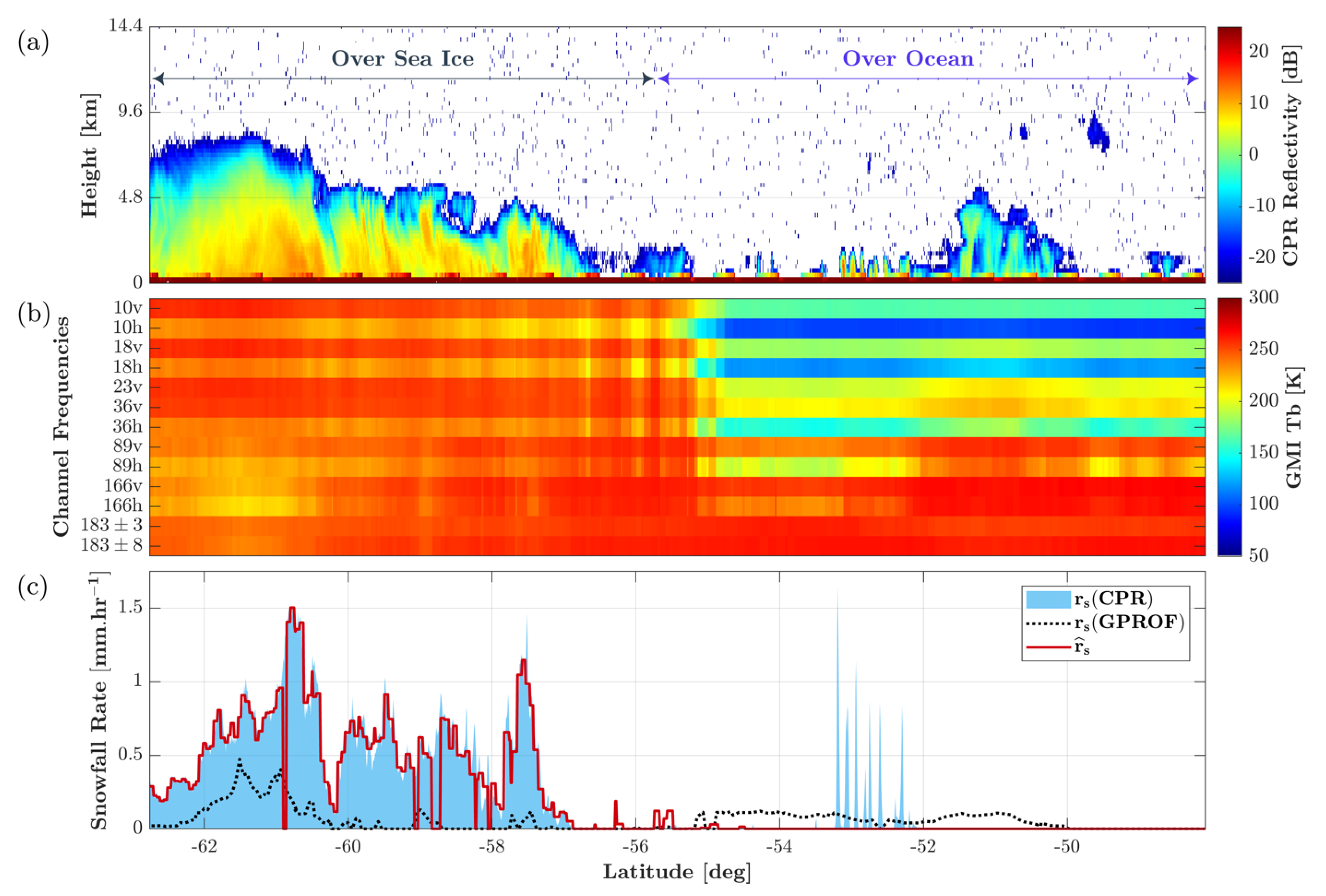
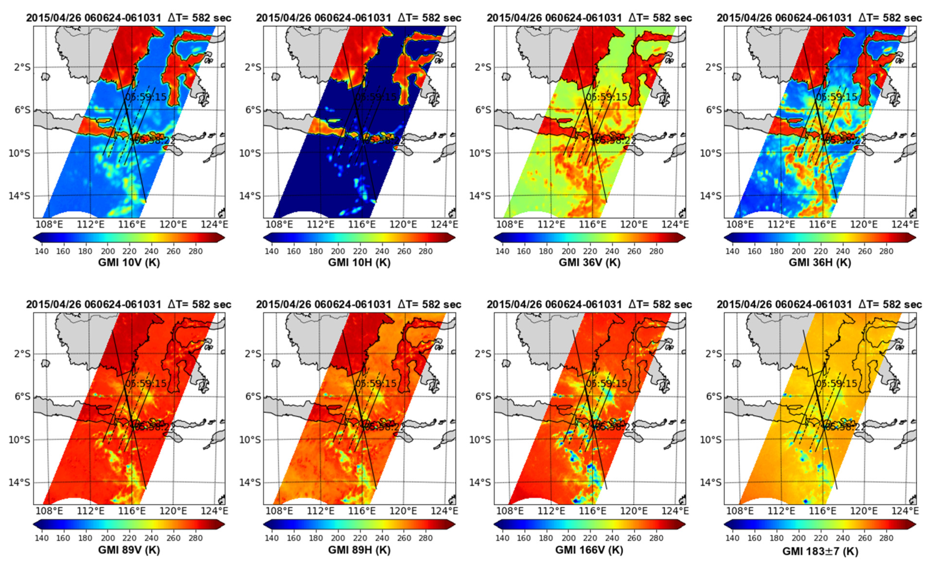
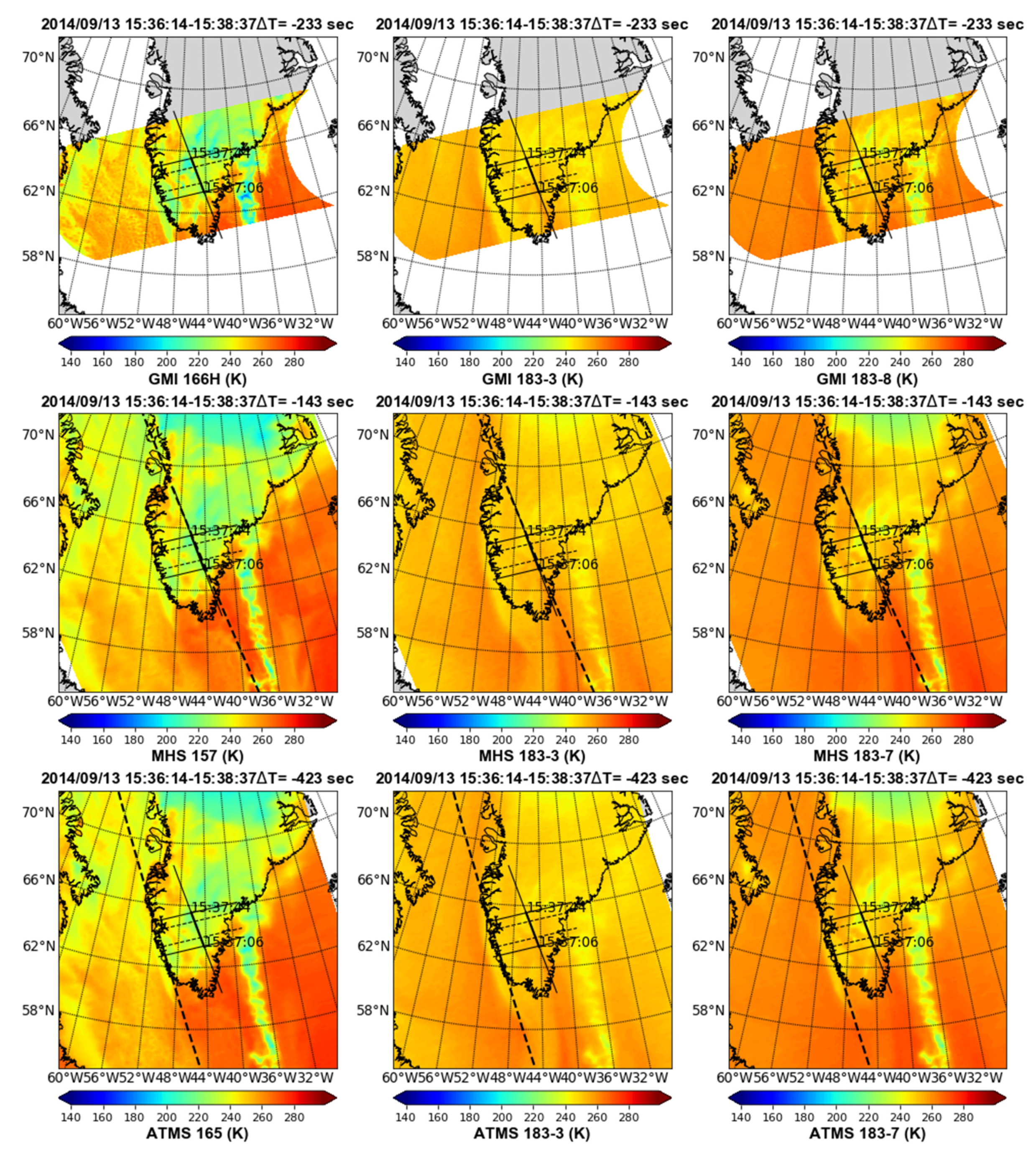
3.1. TB Signatures and Retrieval of High-Latitude Snowfall over Open Oceans and Sea Ice

Even though the DPR has higher space-time coverage than the CPR, evidence suggests that it is not sufficiently sensitive to capture the light snowfall events [25,26]. The high sensitivity of the CPR to low concentrations of snow and ice particles makes it perhaps the most accurate spaceborne instrument for the retrieval of high-latitude precipitation, especially the shallow cumuliform snowfall [27,28], which is the dominant precipitation regime over the polar regions. Therefore, coincidences of CPR (2006-present) and GMI provide a unique opportunity to study microwave signatures of light oceanic snowfall in high latitudes over open oceans and sea ice beyond the sensitivity of the DPR data.

These coincidences can be used not only to understand how the snow cover changes the snowfall scattering over sea ice, but also to construct databases for Bayesian retrieval of light snowfall [29,30,31] and reduce the uncertainty that might exist in passive retrievals in official GPM products [15] that solely rely on DPR-GMI coincidences. Figure 6 shows the results of a Bayesian retrieval algorithm [31] that uses the independent GMI-CPR coincidences to retrieve snowfall of a cyclonic snowstorm moving across the South Atlantic and Indian Oceans toward the coast of Antarctica on 10 October 2014—where CPR crosses the GMI orbit #3498. The storm occurred over both open oceans and sea ice.

The part of the storm over sea ice (latitudes poleward of 55S) is well developed. The narrow, sheared columnar-like CPR reflectivity profiles distributed across this cross-section with values exceeding 10 dBZ (Figure 6a) to almost 7 km of atmospheric depth suggest that the snowfall is largely convective in nature. As shown in Figure 6c, the algorithm with CPR-GMI coincidences captures the snowfall occurrence and rates well, while the official GPM passive MW GPROF product is approximately a factor of two smaller. Over oceans (latitudes equatorward of 55S), radar reflectivity values (Figure 6a) capture a shallow outer snow band (52S-50S region) with narrow, shallow columns and pockets of shallow liquid very near the surface (55S-52S region). In response, any scattering processes from this shallow ice region is masked by the highly polarized surface emissivity in this region (55S-52S latitudes) at 89 GHz, and only a slight residual polarization (166V-166H difference) and TB depression occurs at 166 GHz. As shown, the CPR 2C-SNOW-PROFILE active retrieval algorithm [32,33] estimates sporadic but intense cells of snowfall while both the official GPM product (GPROF) and the presented algorithm fail to capture that narrow snow band. For the GPROF case, the main limitation is the nature of the fundamental low sensitivity of DPR to snow events and the resolution of GMI channels. Additionally, a priori-based estimation techniques require the candidate entries to be as congruent as possible to the environmental and surface conditions at the time of the satellite overpass. Being highly variable, the specific sea ice, snow cover, temperature, moisture structure at the time of this GPM overpass may be undersampled in the a priori database. Even though thorough validation is not possible in such remote areas, considering the CPR snowfall as a relatively more accurate reference, the results suggest that the use of a larger dataset of GMI-CPR coincidences may lead to reduced uncertainty in passive MW-based retrieval of high-latitude snowfall.

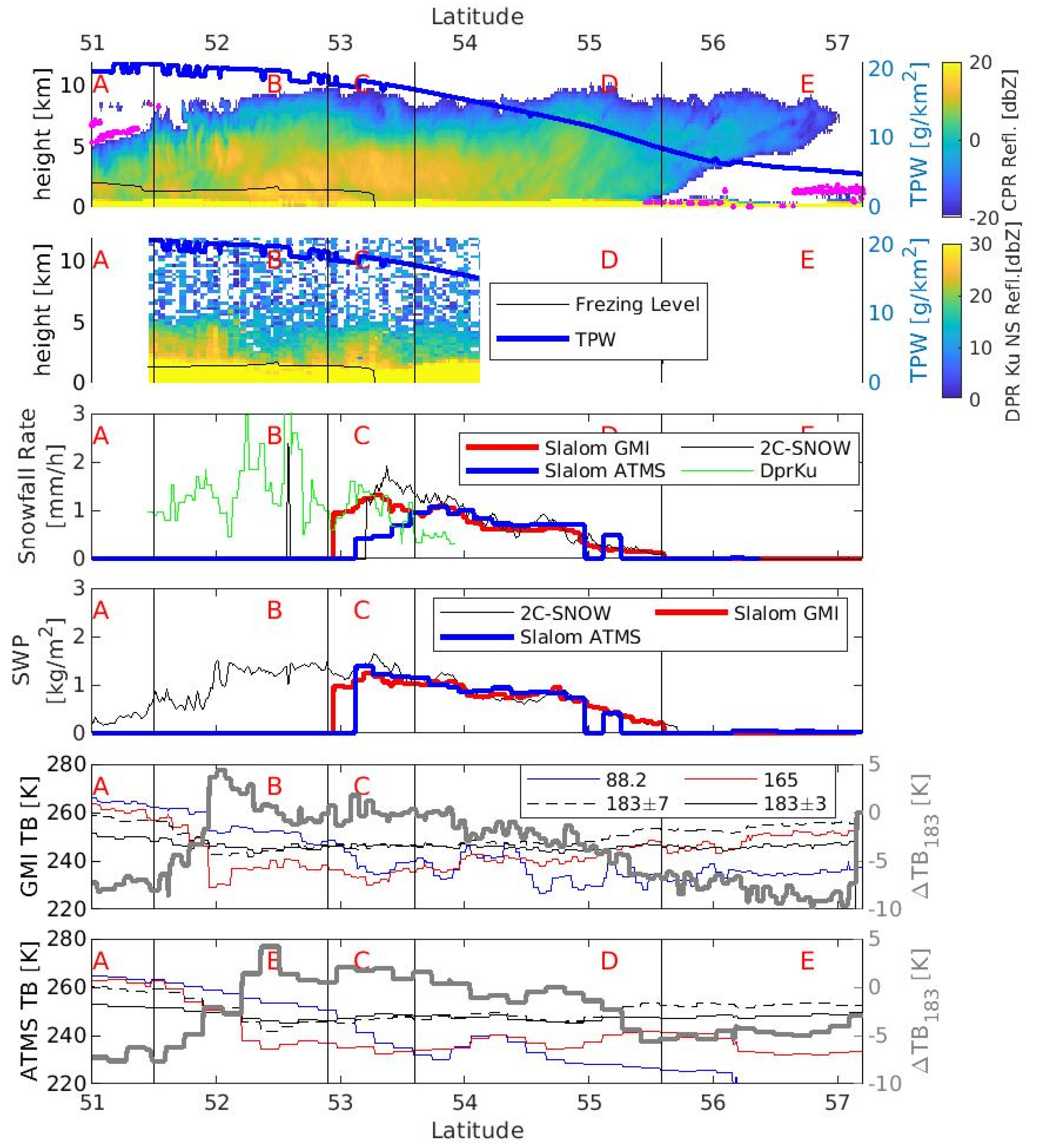
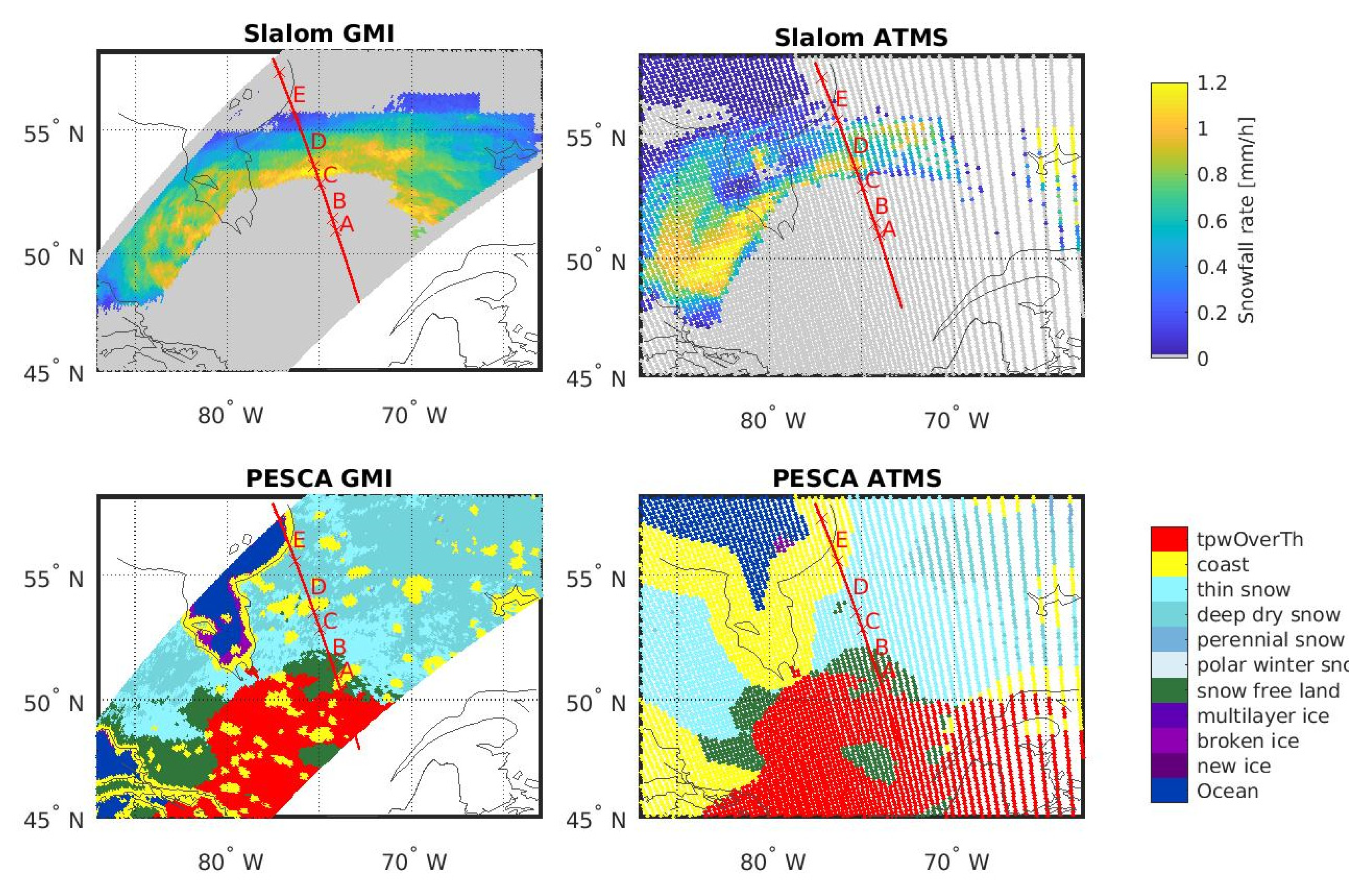
3.2. Exploitation of Cloudsat for Passive MW Snowfall Retrieval Algorithms

The multi-year, quasi-global, and complementary DPR and CPR measurements offer a unique and extensive resource to analyze spaceborne microwave radiometer precipitation observational capabilities. This can be particularly useful in remote areas and/or where ground-based observations are sparse or not available (e.g., high latitudes), and in conditions and regimes where PMW precipitation retrieval is more challenging (e.g., light precipitation and snowfall). A preliminary analysis to assess and identify a reliable reference for snowfall measurements was carried out by comparing various products from GPM DPR and Cloudsat 2C-SNOW-PROFILE from the CloudSat-GPM coincidence dataset described in this manuscript [25]. They concluded that the near global CloudSat coverage and higher sensitivity of the W-band CPR (relative to both DPR radars) make it more suitable for snowfall-related research especially at higher latitudes, although it may be affected by significant attenuation in the presence of intense snowfall [34]. In another study, the potential of the use of the CloudSat-GPM coincidence dataset to improve snowfall detection and retrieval techniques for passive MW radiometers at higher latitudes was described [35]. The analysis of matched GMI and CloudSat CPR snowfall observations (mainly occurring at latitudes between 55° and 65° N) provided insights on microwave multi-frequency signals associated with snowfall. The analysis quantitatively showed the complex interconnection of high-frequency channel response to snowfall with background surface and environmental conditions (e.g., snow cover over land, sea ice concentration over ocean, water vapor content), and with the presence of supercooled droplets (as inferred from CPR and CALIPSO observations). The study also showed how such a response depends on cloud vertical structure and snowfall intensity. Based on these findings, SLALOM [36,37], a new algorithm for GMI to retrieve snow water path (SWP) and surface snowfall rate (SSR), has been developed. The machine learning-based SLALOM algorithm exploits the multi-platform (GPM/CloudSat/CALIPSO) snowfall coincidence dataset, and is based on a random forest approach for snowfall and supercooled water detection, and multi-linear regression and gradient boosting for the SWP and SSR retrieval. Results showed very good skills of SLALOM compared to CPR and to ground-based observations, both in terms of surface snowfall occurrence and quantification [38]. SLALOM complements other studies using the CloudSat-GPM coincidence datasets for passive microwave snowfall retrieval algorithms based on machine learning approaches for AMSU/MHS [39,40].

A similar approach to SLALOM has been recently developed and applied to the ATMS onboard Suomi NPP, NOAA-20, and the future Joint Polar Satellite System (JPSS) platforms. The differences between GMI and ATMS (scan geometry, channel frequencies and spatial resolution) have been taken into account in the algorithm design, where a new global Cloudsat-ATMS coincidence dataset was built and used for training. The algorithm prototype (SLALOM-ATMS) is based on four different neural networks modules for the detection of snowfall and supercooled liquid droplets, and for the estimation of surface snowfall rate and snow water path. It is worth noting that during the development of the SLALOM approach for GMI and for ATMS, the impact of the extremely variable frozen surface conditions (snow-covered or sea ice) on the (weak) passive microwave snowfall signal [41,42,43], including references in [43], has been tackled through the exploitation of the low frequency channels (<37 GHz) available in both radiometers. The Passive microwave Empirical cold Surface Classification Algorithm (PESCA) for GMI and ATMS [44] has been recently developed to be able to detect and characterize snow cover (and sea ice) at the time of the satellite overpass.

The assessment of the performance of SLALOM-ATMS compared with SLALOM-GMI is currently ongoing and is primarily based on the CloudSat-GPM dataset. Triple coincidences between Cloudsat-GPM-ATMS are used for this purpose. As an example, Figure 7 and Figure 8 show an application of the SLALOM algorithms for GMI and ATMS to a snowfall event that occurred over Canada in the Quebec and Ontario region on 24 November 2014. The top two panels in Figure 7 show the cross-section of CPR and DPR Ku-band reflectivity and the associated total precipitable water vapor (TPW) from ECMWF. The middle two panels in Figure 7 show fairly good agreement between the snowfall rate and snow water path estimates from SLALOM (GMI and ATMS) compared with the 2C-SNOW-PROFILE and DPR Ku-band products.

For larger context, Figure 8 shows the maps of the snowfall rate from SLALOM and the surface type characterization from PESCA, comparing the GMI and ATMS retrievals. Several regions are highlighted in the figure with capital letters. Region A is characterized by the presence of relatively high temperature and supercooled droplets (pink dots in Figure 7, panel 1) on top of the cloud outside the area of coincidence between CPR and DPR. Region B is also characterized by relatively warm temperatures (evidenced by the height of the freezing level). In this region, both SLALOM and 2C-SNOW-PROFILE do not detect any precipitation (it is worth noting that these products retrieve only frozen precipitation, and returns no precipitation when liquid or mixed-phase precipitation at the surface is likely), while the DPR-Ku product retrieves solid precipitation. This inconsistency can be attributed to the height of the DPR near-surface bin placed above the freezing level [25]. This feature is noticeable through examination of the second panel. Region C is characterized by an abrupt decrease in the freezing level and by the transition from rainfall to snowfall. All the algorithms in this region show some inconsistencies in the snowfall rate estimate and in detecting the separation between snowfall and rainfall. By contrast, Region D is characterized by colder temperatures and dry snow at the surface. In this region, SLALOM (both for GMI and for ATMS) and 2C-SNOW-PROFILE show a very good agreement in both snowfall rate and snow water path (SWP); some differences can be noted between SLALOM-ATMS and 2C-SNOW in Region D at latitudes higher than 55 degrees, mainly due to the relatively lower spatial resolution of ATMS that causes some underestimation of lower snowfall rates. In Region E, all algorithms agree and do not detect any snowfall. In general, the maps of SLALOM snowfall rate for GMI and ATMS in Figure 8 show a good agreement of the retrieval from the two radiometers, with some differences mainly linked to a slight overestimation of the intensities and a larger snowfall area by SLALOM-ATMS with respect to SLALOM-GMI. The maps of the surface characterization from PESCA are very consistent, especially for the detection of snow-covered areas (the red areas depict the region where PESCA is not applicable due to the high temperature and/or moisture conditions [44]). The main differences are in the thickness of the coastal areas (where PESCA is not used), due to the different IFOV size of ATMS and GMI.

These findings, and the increasing use of CloudSat-based observational datasets for passive MW-based snowfall retrieval, are promising results towards the effective exploitation of passive MW radiometry for snowfall global monitoring from the future European EarthCare (W-band radar), and the and EPS-SG polar program, which will deploy the Microwave Sounder (MWS) and the Microwave Imager (MWI)/Ice Cloud Imager (ICI) radiometer combination on the A and B satellites, respectively [45].

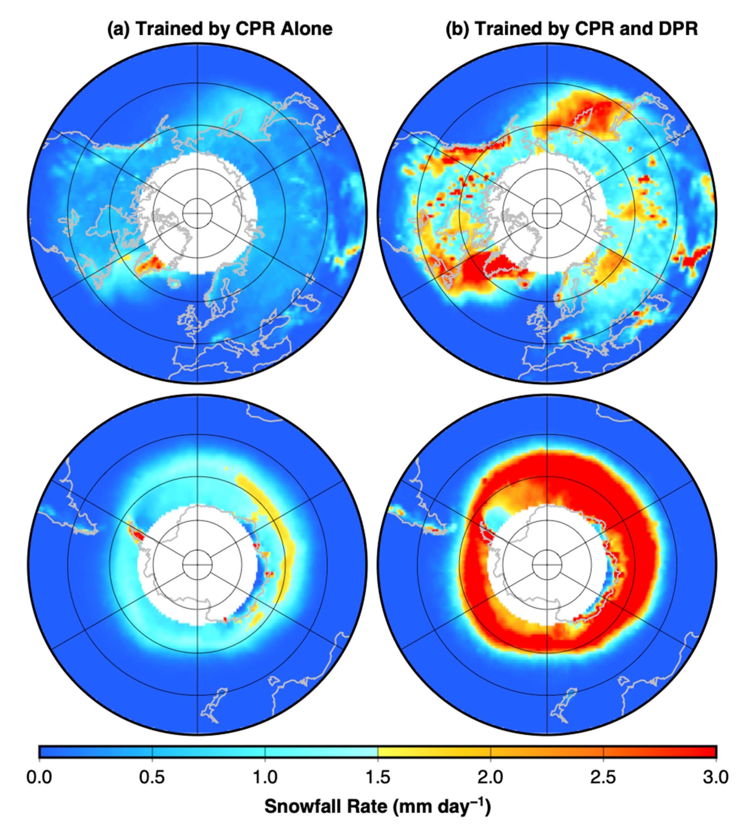
3.3. High Latitude Snow Detection and Distribution

The detection of falling snow and retrieval of its snowfall rate from passive MW observations suffer from several obstacles, such as the uncertainty of surface emissivity, insufficient strength of the ice scattering signal in the TB observations, and masking of the ice scattering by (absorbing) cloud liquid water emission. On the other hand, since radars measure hydrometeor backscatter at individual range gates (except for ground clutter contamination near the surface), the snow scattering signature can be unambiguously detected by a radar if it is designed with a sufficient low threshold of minimum detection such as the CPR on CloudSat. As demonstrated in earlier sections, the CloudSat CPR is considered to be an effective sensor for snowfall detection and retrieval [26,33]. However, because of its narrow spatial coverage and short duration of data availability, many research and operational applications cannot rely on CloudSat data alone. Therefore, there is a need to exploit the radar and radiometer data contained in the collection of CloudSat-GPM coincidences, to further improve and characterize the snowfall estimates from current passive MW sensors such as GMI, ATMS and MHS.

The CloudSat-GPM coincidence dataset has been used as a training set in several snowfall retrieval studies. A physically optimized a priori database for a Bayesian GPM GMI snowfall retrieval algorithm over ocean has been developed [46]. To build the database, CloudSat CPR-derived snow water content profiles are used as initial input to a radiative transfer model. Radiative transfer simulations are then performed to seek the best consistency between coincident CPR and GMI observations using a one-dimensional variational (1DVAR) method. An interesting finding from this study was that the largest remaining biases in the simulated GMI brightness temperatures often occurred for shallow snow cloud cells or very deep convective snow clouds [47], which are hypothesized to be due to uncounted rich cloud liquid water in the shallow clouds and uncorrected attenuation to CPR reflectivity in deep clouds. The database is then applied to a Bayesian retrieval algorithm to study the climatology of snow water content profiles over global oceans.

A technically less rigorous, but more broadly applicable (e.g., over any surface types) snowfall detection and retrieval method was proposed by [48], in which the radar-derived snowfall rates are used as truth to train passive MW TB observations. In this framework, the primary information contained in the multichannel microwave TB are presented in the three leading principal components (PCs) derived by an empirical orthogonal function analysis. Using radar and radiometer observations in the coincidence dataset, the probability and the rate of snow precipitation are computed and represented as a three-dimensional lookup table with the three leading PCs as its axes. In generating the lookup table, the method of [49] is used to separate snow and rain, and either the CloudSat CPR retrieval [33] alone or the combined CloudSat CPR and GPM DPR [7] retrieval is considered as the true snowfall rate. Combining the CPR and DPR retrievals can mitigate the shortcomings of the low detectability of the DPR for light precipitation and the attenuation/saturation of the CPR for heavy snow events [35,50]. Figure 9 shows the global snowfall distributions derived based on this method from 5 years of GMI data from 2014 to 2019.

In the left panel of Figure 9, snowfall rates are based on the lookup table generated using the CPR snowfall retrieval alone as truth, while on the right, snowfall retrievals are based on the lookup table generated by combined CPR and DPR as truth. In the CPR and DPR combination, CPR retrievals are used when DPR reflectivity is below its minimum detection threshold (assumed at 13 dBZ); otherwise, DPR retrievals are used. The reason for adapting such a combination is that the CPR is more sensitive to light snow and the DPR is more accurate for retrieving heavy snow. Clearly, the two sets of the retrievals display a similar pattern of global snowfall distribution, such as the snowfall bands along the storm tracks in the northern hemisphere and the circular snowfall pattern in the southern hemisphere. However, the snowfall rates based on the combined CPR and DPR trained lookup table are much larger than those based on the CPR trained lookup table. From these discussions, it is argued that the results based on the combined CPR and DPR trained lookup table (the CloudSat-GPM coincidence dataset described in this study) should more faithfully represent high latitude snowfall amounts and patterns.

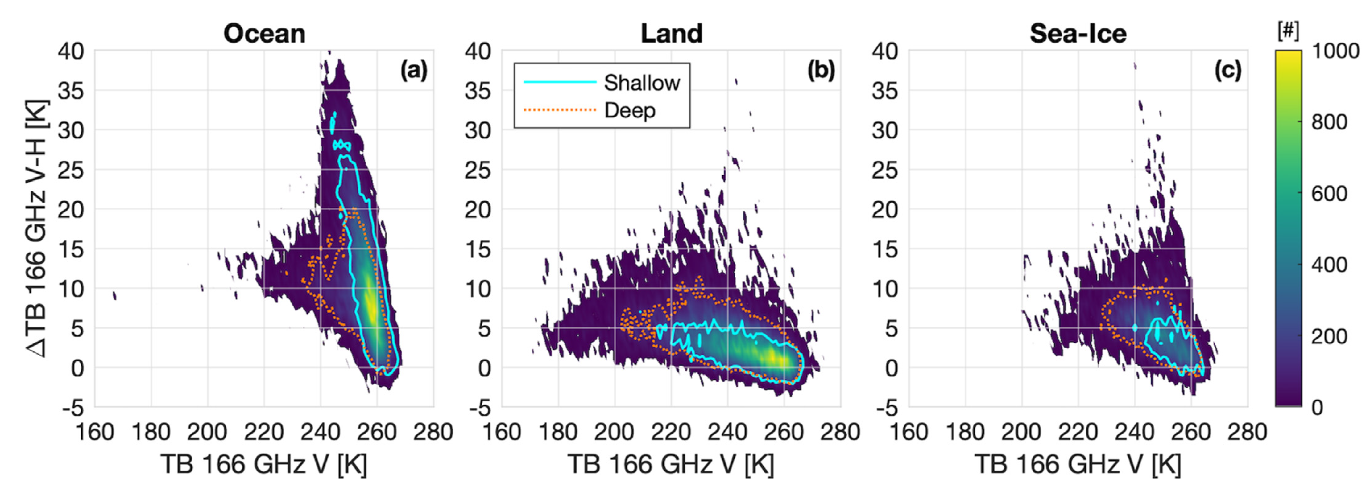
3.4. TB Signatures Due to Shallow Cumuliform and Deep Stratiform Snowfall Regimes

Surface snowfall can be produced by a variety of forcing mechanisms that are accompanied by different in-cloud physical processes and microphysical composition. CloudSat-only observations have enabled a near-global accounting of different snowfall regimes. For instance, shallow cumuliform snowfall forced by marine cold air outbreaks shows distinct geographic and seasonal signatures and plays in important role in annual snowfall production in many regions worldwide [27,28,51]. Coincident CloudSat-CALIPSO observations confirm that oceanic regions exhibiting frequent shallow cumuliform snow are typically composed of mixed-phase cloud and precipitation particles [52] and display passive microwave TB behavior that is dominated by cloud liquid water emission [53], while combined GPM radiometer and surface radar studies of intense shallow cumuliform events indicate significant ice particle scattering signals at the highest GPM radiometer frequencies [54]. The coincident CloudSat-GPM dataset is an ideal tool for further exploring different TB signatures associated with shallow cumuliform and deeper stratiform snowfall regimes, thus improving the ability for radiometer-based retrievals to produce accurate quantitative precipitation estimates for different snowfall categories.

In Figure 10, 2D-histograms of the 166 GHz polarization difference ΔTB (defined as the difference between the 166 GHz vertical (V) TB minus the 166 GHz horizonal (H) TB) vs. the 166V GHz TB are shown for deep stratiform (orange dotted lines) and shallow cumuliform (cyan solid lines) for different surface type. Cloud classification information from the CloudSat 2B-CLDCLASS product that is contained with the 2B-CSATGPM product allows these two snowfall regimes to be easily identified and inflates the scientific value of the ensuing analysis [27]. Over ocean, the distribution of deep stratiform pixels shows a larger concentration of higher 166 GHz combined with higher ΔTB values (Figure 10a, orange dotted line), highlighting the contribution of ice scattering in deep precipitating structures. Oceanic shallow snowfall (Figure 10a, cyan solid line) shows a very polarized signal (exceeding 30 K) and very warm TBs (250–270 K) compared to deep stratiform snow. The extremely dry environmental conditions associated with very shallow precipitation structures allows the high-frequency (166 and 183 GHz) GMI channel atmospheric weightings to peak lower in the atmosphere [54]. Upwelling microwave radiation therefore originates from lower within the atmosphere, with the very polarized oceanic surface contributing to the high observed ΔTB.

For the same reason, the less polarized land surface (Figure 10b), most likely covered by snow, contributes to the more variable 166 GHz TBs showing much less polarization (ΔTB < 5 K) for shallow cumuliform structures (cyan solid line). Many shallow cumuliform snowfall events are produced by mixed-phase clouds and contain ample supplies of supercooled cloud water that effectively temper the ice scattering signature. This effect likely causes the large cluster of over-ocean ΔTB observations less than 10K. Deeper TB depressions are found for deep stratiform clouds over land (Figure 10b, orange dotted line), although some contribution from ice scattering is still significant with ΔTB reaching 10 K. The signal over sea ice (Figure 10c)—a notoriously difficult underlying surface for passive microwave precipitation retrievals—lies in between the ocean temperatures (240–270 K) and the land polarization signal (ΔTB up to 10 K).

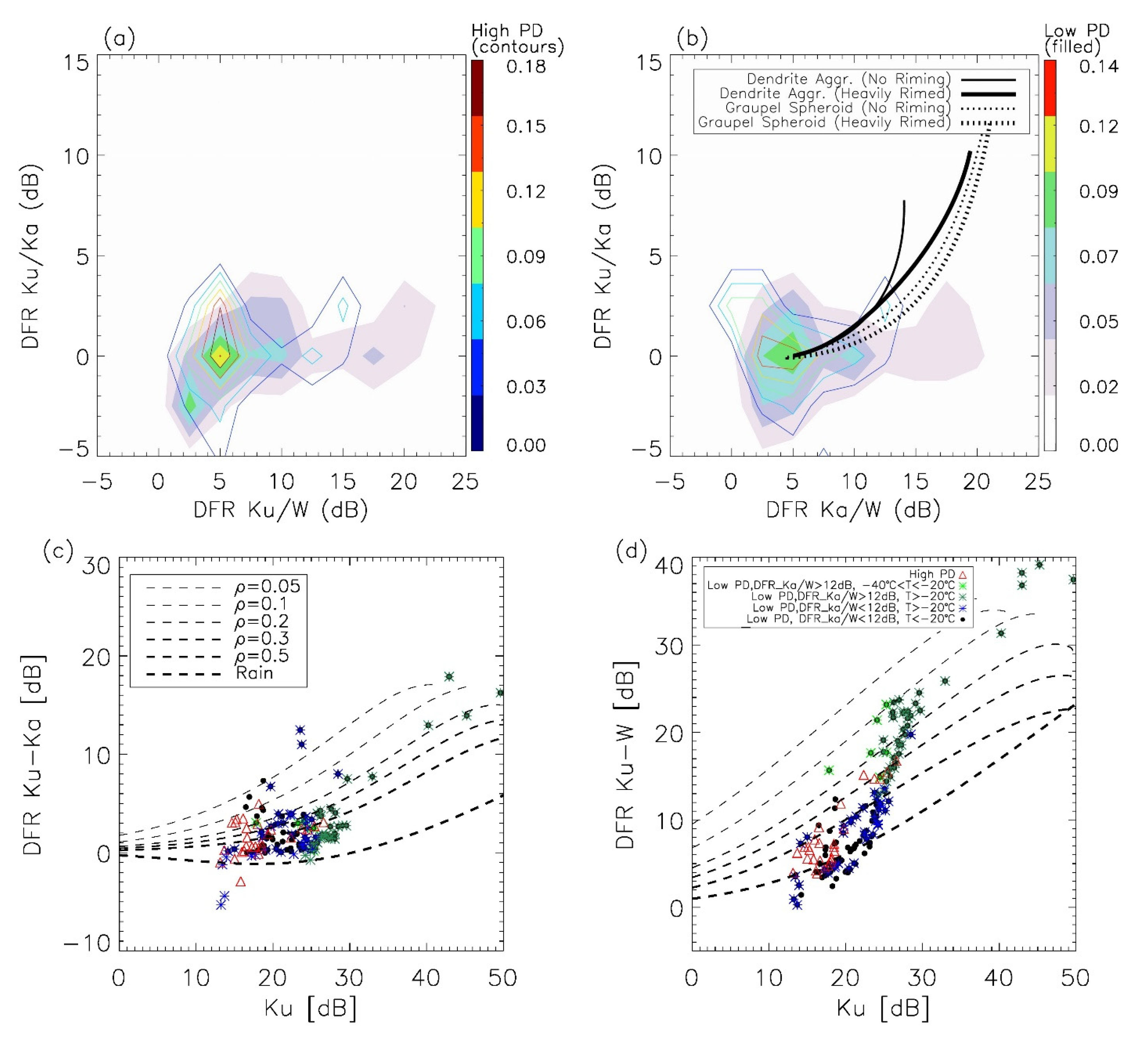
4. Cloud and Precipitation-Sized Ice Microphysics

The discussion in Section 3 focused on the use of the CPR to account for the limited sensitivity of the DPR Ku- and Ka-band radars to near-surface cold-season precipitation. Similarly, the limited sensitivity of the DPR also masks the detection of upper-level ice (see top panels of Figure 4). In this section, the use of the CloudSat-GPM coincidence dataset is investigated as a means to study the characteristics of ice crystals that are commonly noted above convective cloud systems.

4.1. Ice Crystal Habit and Orientation

The CloudSat-GPM collocated dataset provides a unique opportunity to (1) validate space capability of applying multi-frequency radar theorem and algorithms that were previously developed based on ground or airborne measurements, and (2) explore the hidden ice microphysical information in high-frequency passive radiometer measurements that were previously unavailable or overlooked. Both practices are illuminating for future satellite mission development and selection.

Cloud ice and snow microphysical characteristics, mainly particle size distribution (PSD), shape and density, are complex and vary widely in different regions and weather systems [55]. It is critical to measure and simulate these properties accurately for better constraint of the cloud radiative effect (CRE) as well as for better the prediction of surface precipitation details such as phase, intensity and onset time. As different frequency radars are sensitive to different parts of the size spectrum, multi-frequency radar joint observations were proposed for ground instrumentation as early as 2004 [56]. Theories and retrieval algorithms have been developed ever since to retrieve ice microphysical characteristics from the “triple-frequency diagram”, which is essentially mapping the dual-frequency ratio (DFR, radar reflectivity difference) observations on the pre-computed look-up-table [57,58,59]. This approach has been demonstrated to be powerful through comparison against in situ measurements [60,61], where collocation amongst the different radar beams is more readily achieved compared to the collocation obtained from the separate DPR and CloudSat beams.

The CloudSat and GPM-DPR (Ku and Ka) collocated measurements provide the first “pseudo-triple frequency” radar dataset from space that has been used to study cloud ice microphysics. This dataset was used to differentiate distinct ice microphysical regimes for stratiform and convective clouds, respectively [62]. In [63], it was used in conjunction with collocated GMI 166 GHz polarimetric observations to uncover ice crystal orientation information. The positive polarization difference (PD) signals between GMI 166 GHz vertically and horizontally polarized radiance observations were attributed to the dominantly horizontal orientated large cloud ice or snow particles, which are found to frequently occur in anvil and stratiform cloud layers [64]. PD measurements are further separated into “high-PD” and “low-PD” groups [63], and collocated CloudSat and DPR DFRs are composited on the triple-frequency diagram, as shown in Figure 11a,b (colored shades for “low-PD” and colored contours for “high-PD”). In comparison to radiative transfer model (RTM) simulations (black curves) that can usually well-capture the variabilities of ice microphysics from ground and airborne observations, the spaceborne observations are far more diverse, which are attributed to factors such as imperfect collocation, beam-filling and footprint inhomogeneity. On the one hand, quantifying impacts from these factors is a challenge for future spaceborne radar retrieval algorithm development.

On the other hand, these pseudo triple-frequency radar measurements are extremely useful in delineating ice microphysics information embedded in the passive PD signals. As suggested by the difference between the “high-PD” and “low-PD” statistics in Figure 11, “high-PD” scenes likely contain more horizontally oriented, dry fluffy snow aggregates in the stratiform layer, while “low-PD” scenes correspond to either small ice crystals in anvil clouds, or denser spheroids that may experience some degree of riming. With the aid from ECMWF-AUX data that are provided in the CloudSat-GPM collocation dataset (Appendix A), the former scenario was likely associated with the decaying stage of the mesoscale convective system, and a positive PD–surface precipitation intensity relationship was found for the “high-PD” scenes [63]. This paper pointed out that an alternative cost-efficient way to replace the multi-frequency spaceborne radar is to use multi-frequency polarized high-frequency passive microwave and sub-millimeter radiometer observations. Based on the observational evidence provided in [63], an ice crystal orientation induced longwave radiative mechanism that facilitates (prohibits) the water vapor depositional growth of horizontally (vertically) aligned ice crystals was proposed [65]. Collocated GMI and CloudSat observations are found to support this mechanism.

While currently only GMI offers this high-frequency PD capability, such observations will be made available from near-future missions such as the Ice Cloud Imager (ICI) that will be deployed upon the Metop-SG satellite system [45], and from airborne-based campaigns. The Investigation of Microphysics and Precipitation for Atlantic Coast-Threatening Snowstorms (IMPACTS) is a multi-year campaign to study winter storms that affect the eastern seaboard of the United States. Across three six-week deployments, the NASA ER-2 and P-3 aircraft carries a range of remote sensing and in situ instruments, supported by ground-based and satellite measurements. The suite of remote sensors on board the ER-2 include four radar bands from three sensors: the ER-2 X-band Radar (EXRAD; X-band), the High-Altitude Imaging Wind and Rain Airborne Profiler (HIWRAP; Ku- and Ka-band), and the Cloud Radar System (CRS, W-band). The Conical Scanning Millimeter-wave Imaging Radiometer (CoSMIR) provides millimeter-wave brightness temperatures from 50 to 183 GHz, including dual-polarized observations at 89 and 166 GHz. The first deployment occurred during the winter of 2019–2020 and during the final year (scheduled for winter 2022–2023), the campaign plans to fly the Configurable Scanning Submillimeter-wave Instrument/Radiometer (CoSSIR; formerly Compact Scanning Submillimeter Imaging Radiometer), which is currently being upgraded to measure dual-polarized brightness temperatures at eight frequencies between 170 and 684 GHz.

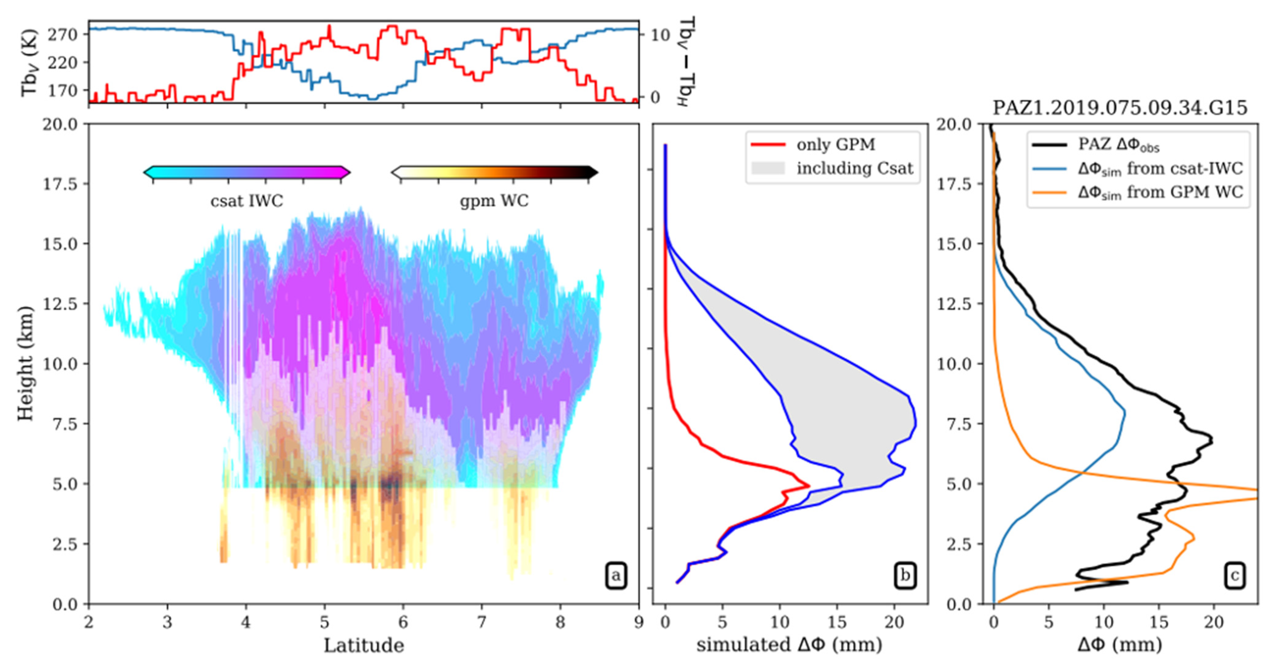
4.2. GNSS Differential Propagation Phase through Ice Media

A unique use of the CloudSat-GPM data has been able to explain the Global Navigation Satellite System (GNSS) polarimetric radio occultation (PRO) data collected from the Radio Occultations through Heavy Precipitation (ROHP) receiver, located onboard the Spanish PAZ satellite launched in early 2018 [66]. The PRO technique enhances standard RO by measuring GNSS signals at two orthogonal linear polarizations (H and V). Owing to hydrometeor asymmetry, a cross-polarized component is induced as the circularly polarized 1.4 GHz GNSS carrier signal propagates through regions of heavy precipitation, measured as a differential phase delay (Δϕ) by ROHP’s dual-channel receiver. The recent examination of the nearly three years of ROHP data has revealed that the PRO technique detects horizontally oriented frozen particles well above the freezing level, above deep convective clouds, within upper-level regions where ice crystals are too small to be detected by the GPM-DPR radars [67]. The PRO technique augments the traditional thermodynamic parameters (temperature, pressure and water vapor) available from RO, with an indication of precipitation along the GNSS propagation path [66].

To validate these observations, the CloudSat-GPM coincidence dataset was used to build a look-up-table of vertical profiles of CloudSat-retrieved ice water content (IWC), based on the coincident information from GMI. In this way, IWC 3-dimensional fields can be used to simulate Δϕ based only on collocations between PAZ and GPM, and compare them with actual Δϕ observations [67]. Figure 12 presents one example from a ROHP observation on 16 March 2019, where a good agreement is found above the freezing level when the CloudSat-retrieved IWC is used, whereas the lower layers are better reproduced when using the Ku-band (NS) GPM combined algorithm (CORRA) [8] water content to perform the Δϕ simulations. These findings suggest the capability of polarimetric RO to resolve the height of high-level ice water path, complementing the traditional RO profile estimates of temperature, pressure and water vapor.

5. Light Precipitation and Surface Emissivity Related Effects

5.1. Accounting for Light Precipitation in the GPM Combined Radar—Radiometer Precipitation Profile

A major goal for future updates to GPM-based precipitation products is to enhance existing precipitation algorithms for the GPM constellation with retrievals of light precipitation (snow and drizzle), below the sensitivity of the active DPR radar, using information content from the passive sensors and providing a crucial missing component in the full suite of GPM products. The Southern Ocean, with its relatively homogeneous background, high frequency of drizzle, and known retrieval discrepancies [68], serves as a testbed. Understanding the full distribution of precipitation is a vitally important component in understanding global energy and water cycles and their variability.

The addition of light precipitation to GPM products is carried out using an optimal estimation-type (OE) non-raining cloud and water vapor retrieval [41], with development and testing over the Southern Ocean. Non-convergence of the OE retrieval in areas with no detectable radar signal is used to identify areas with a high probability of light precipitation. The other component of the retrieval is a more process-oriented microphysical characterization of the light precipitation, which is explored using information derived from the higher sensitivity CloudSat mission along with model information to identify associated atmospheric state and dynamics. In versions 1–5 of the GPM Combined (CMB) Radar–Radiometer retrieval algorithm (CORRA) [8], a retrieval is only performed where the detected return from the active DPR indicates the presence of precipitation. Since the CORRA algorithm is run after the DPR Level 2A processing, it is denoted as the 2B.GPM.DPRGMI.CORRA product at the PPS archive (often denoted simply as 2B-CMB). An upcoming version will incorporate a non-raining optimal estimation (OE) retrieval (described in Section 3 of [42]), making the product more easily adaptable to GPROF database construction and the two products generally more consistent. Screening for the occurrence of light precipitation can therefore be implemented within this framework. The cutoff value of chi-squared (or normalized cost function) will be determined using CloudSat-GPM coincident overpasses from the coincidence dataset described in Section 2, which contains all radar and radiometer data for CloudSat-GPM orbit coincidences. Light precipitation will be assumed in areas where there is no radar return, but the OE is unable to converge.

The second piece of 2B-CMB implementation involves determining the microphysical characteristics of the retrieved light precipitation profiles. This will be carried out offline from the 2B-CMB code and will test two approaches, with the most successful to be presented for implementation in the main retrieval. Both start with the database of CloudSat coincidences. Based upon the chi-squared cutoffs determined in the previous step, reflectivity profiles from CloudSat will be used along with associated hydrometeor profile retrievals. These profiles will be analyzed to determine whether generalizations of hydrometeor amount and profile shape (with phase determined by temperature) can be applied in a bulk sense, under atmospheric constraints, or are sufficiently unique to require a Bayesian retrieval within the light precipitation areas using a database derived from the CloudSat profiles with the goal of accurately reproducing the multi-spectral GMI signal from the light precipitation. These outcomes can all be easily implemented, and will be determined based upon results from the previous steps.

An example of a typical matchup over the Southern Ocean is shown in Figure 13. The top 3 panels show reflectivity along the CloudSat path for CloudSat (top), and the two DPR frequencies. There is light precipitation signal across much of the first half of the swath observed by CloudSat but below the DPR sensitivity. The TB for two GMI frequencies (166 and 183 GHz) indicate a clear scattering signal in both channels associated with the light precipitation, making it likely these would be flagged by chi-squared in the OE retrieval and provide an excellent test case for defining the eventual retrieval. It is important to note as a caveat here that CloudSat also has a sensitivity threshold and misses some light precipitation (in particular near the surface), so the resulting algorithm will be limited to this level under the construction described here. Once implemented within the framework of the combined algorithm, retrieved drizzle and light snow will be transferred through the GPROF database scheme to the full GPM constellation.

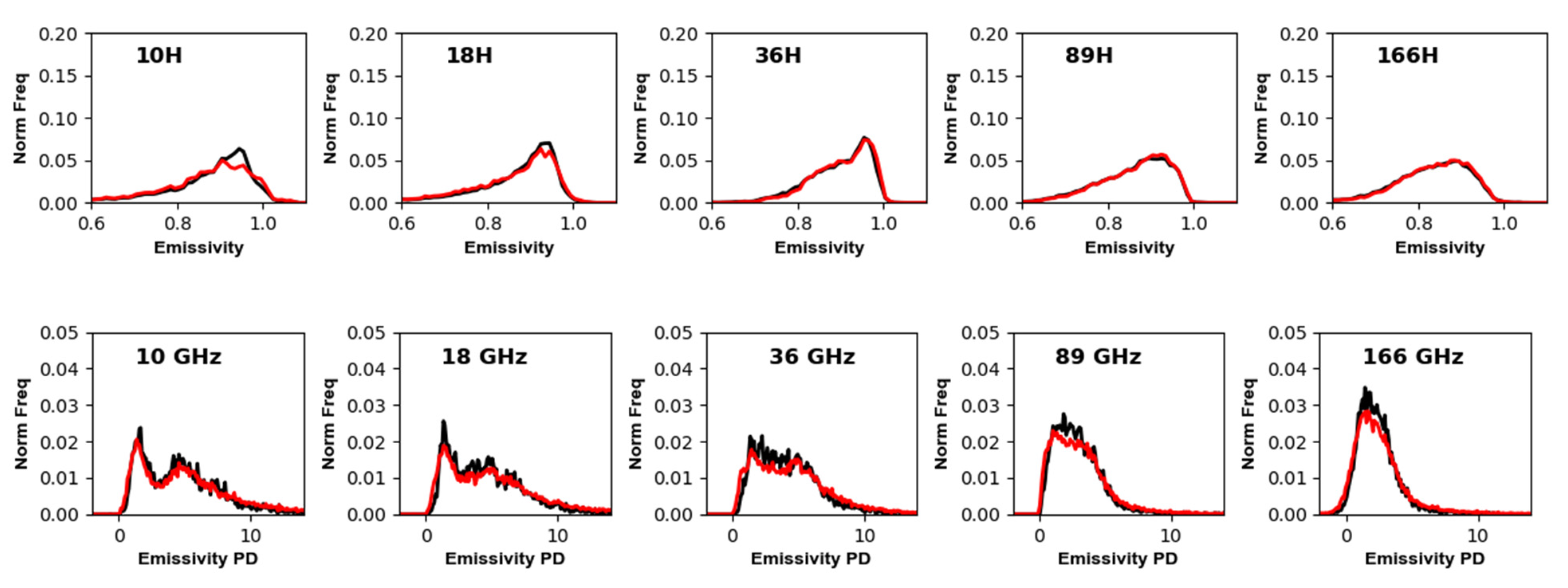
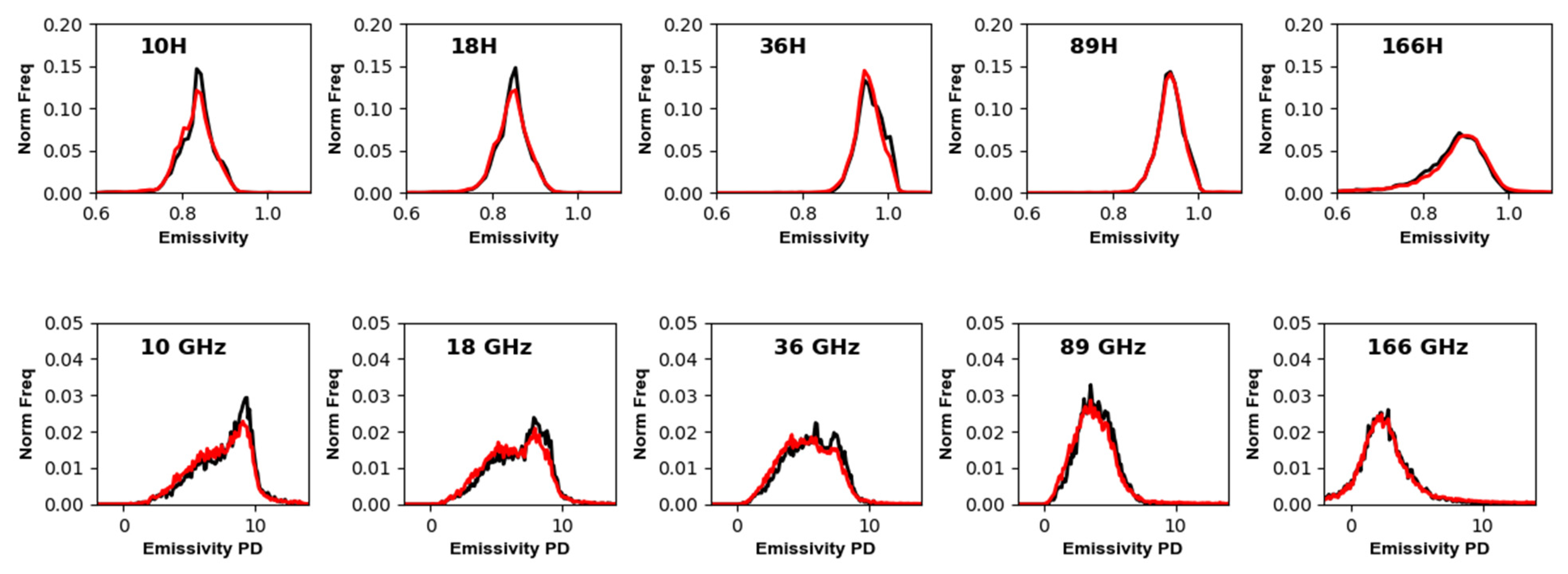
5.2. Cloud Effects on the Estimation of Surface Emissivity Variability

The discussion in the previous sections has largely been directed at the use of the CloudSat-GPM coincidence data for the detection of precipitation that is missed by the GPM radars. Conversely, CloudSat’s superior cloud detection capability (relative to DPR) is also important for identifying “cloud-free” scenes. A large collection of cloud-free GMI (and other passive MW) observations is required to examine the underlying surface emissivity. The DPR is largely transparent to the presence of cloud liquid water, whose absorption properties influence the net upwelling TB, especially for channels above 90 GHz. With cloud-free scenes, the remaining contribution to the upwelling TB is the intervening absorption from constituent gases, which is well-known from microwave transmission models [69] and whose inputs can be obtained from nearby-time weather forecast models or climate model reanalyses. At high latitudes, cloudiness is persistent and can impact the estimation of the surface emissivity at 89 GHz and higher, and a cloud “masking” scheme is needed. The International Satellite Cloud Climatology Program (ISCCP) cloud mask was used by [70], derived from infrared satellite observations. For GPM passive MW precipitation estimates based on knowing surface properties, it is important to know the multi-channel surface emissivity at (or as close to) the time of the satellite overpass, especially surfaces where the surface is highly variable.

To highlight, two surface conditions are isolated: snow/ice cover, and light vegetation. For the latter, only CloudSat-GPM profiles that are identified with a value of the DPR snowCoverMask of 2 (ice) or 3 (snow) are considered. DPR “cloud-free” conditions are defined when no DPR Ku-band radar bins exceed 20 dBZ anywhere in the DPR profile. CloudSat “cloud-free” conditions are defined separately, when no clouds are identified from the 2B-GEOPROF-LIDAR cloud layer product [17], nor from the MODIS-AUX cloud mask. Since the same DPR profile is repeated for every ~5 CloudSat beams (Section 2), this no-cloud condition must also be true for the 10 CloudSat profiles on either side of the CloudSat-GPM profile under consideration.

For its five channels with both H and V polarization, Figure 14 shows the normalized histograms of the GMI H-polarized surface emissivity and its associated emissivity (e) polarization difference (PD), defined as $PD=100\ast \left(e^V-e^H\right)/\left(e^V+e^H\right)$. The CloudSat- and DPR-based values (black and red lines, respectively) are contrasted. If the two curves are close to each other, this implies that the use of DPR alone is sufficient for identifying cloud-free surface emissivity scenes.

Figure 14 shows the variability in the H-polarized emissivity is fairly broad, extending between 0.6 to near unity, with a double peak in the PD, especially at 10 and 18 GHz. Despite some differences near the peak of the 89 and 166 GHz PD histograms, the estimates based on cloud-clearing from DPR and CloudSat are well matched.

Figure 15 shows the same, but for all surfaces where the surfaceTypeIndex in the 2A.GPM.GMI.GPROF file has a value of 6 or 7 (lightly vegetated, see

Table A3. Values of the surface type index and the associated surface characteristics, used in the GPM radiometer-only precipitation algorithm GPROF.

Index	Description
1	Ocean
2	Sea ice
3–7	Decreasing level of vegetation
8–11	Decreasing snow cover
12	Inland water
13	Coast
14	Ocean-sea ice boundary

). The H-polarized emissivity is more peaked near a value of 0.85 to 0.9, depending upon frequency. The shape of the PD histogram at the 10H and 18H GHz channels is opposite that noted in Figure 14 (weighted towards a larger PD for light vegetation than for snow/ice coverage). However, in general, there is good agreement between the two histograms. The results (from these two surface types) imply that an assumption of a 20 dBZ threshold for DPR Ku-band radar is sufficient for identifying cloud-free conditions needed to estimate surface emissivities.

6. Discussion

This manuscript has outlined three application areas whereby the three-frequency (Ku-, Ka- and W-band) radar profiling capabilities offered by coincident CloudSat and either of GPM (2014-current) or TRMM (2006–2014) are used for the improvement or validation of passive/active precipitation retrieval algorithms. It is recognized that there may be additional uses of these data not captured in this manuscript. For light to moderate precipitation, CloudSat provides a more complete top-to-bottom radar-observed vertical structure, including upper and lower portions of the clouds that are not sensed by the GPM DPR (TRMM PR). This latter capability was demonstrated to be useful to improve the representation of cold-season precipitation from passive MW sensors such as GMI and ATMS, and to better account for light rain and drizzle in a future version of the GPM combined radar–radiometer algorithm. CloudSat’s sensitivity to upper-level ice was used to examine polarization signatures noted in GMI high-frequency TB channels and polarized radio occultation observations. The superior capability of CloudSat for masking cloudy conditions was used to identify cloud-free scenes and better isolate microwave surface emissivity retrievals from radiative transfer modeling.

7. Conclusions

In August 2020, CloudSat was moved to standby mode operations (suspended science data collection) after suffering a failure of one of its three remaining reaction wheels. It is unlikely that even with a return to daylight-only operations, a substantial amount of additional CloudSat-GPM data could be collected. Provided that GPM is functioning into operations of the future Earth Clouds, Aerosols and Radiation Explorer (EarthCARE) [71], the opportunity will arise for the collection of additional three-frequency radar profile data with its (Doppler-capable) Cloud Profiling Radar (CPR), that would collect data during the orbit day and night side. EarthCARE is slated to be in a near-polar, low inclination synchronous orbit with an orbital repeat and local time similar to the A-Train configuration. Currently, the CloudSat-TRMM day/night time data extend only until 2011 (prior to GPM), limiting studies relating to diurnal characteristics of clouds and precipitation at latitudes poleward of 35 degrees latitude.

While CloudSat and the EarthCARE CPR provide nadir-only radar profiles, technologies have been rapidly advancing, which may provide future spaceborne multi-frequency radar profiles with an across-track scan capability [72]. Recent years have witnessed the rapid miniaturization of millimeter (mm)-wave and sub-mm wave electronics and hardware suitable for spaceflight to enable Earth science investigations [73]. These technologies provide the potential to host scanning passive MW sounders [74], and Ka-, W- and G-band (183 GHz) profiling radars [53,75] on small, low Earth-orbiting (LEO) satellite platforms suitable for more limited duration, targeted science investigations.

The discussions in this manuscript have largely focused on the use of the three-frequency CloudSat/TRMM and CloudSat/GPM data to assess and improve the GPM precipitation algorithms. In addition, a continuous collection of spaceborne radar profiling observations collected from joint W-band and (at least one of) Ku- or Ka-band observations provides a unique observational to compare against weather and climate model-based simulations of these same profiles, to better constrain amongst parameterizations employed in current models (e.g., [76]). The cloud convective precipitation (CCP) processes whereby the transport of water vapor influences condensation, the growth of clouds into precipitation and the feedbacks within this exchange across water phase transitions identified as a designated observable within the recent NASA Earth Science Decadal Survey [9] are not readily tracked with radar reflectivity observations alone. A spaceborne Doppler capability (to be provided by the EarthCARE CPR) would provide additional dynamical information to improve the separation of radar profiles into convective and stratiform conditions, which is currently carried out with reflectivity observations [77]. The ability to classify passive MW satellite observations into (even crude) distinctions between these two conditions has been identified as one of the leading factors towards the improved representation of the precipitation vertical structure [78].

References

1. Hamada, A.; Takayabu, Y.N. Improvements in Detection of Light Precipitation with the Global Precipitation Measurement Dual-Frequency Precipitation Radar (GPM DPR). J. Atmos. Ocean. Technol. 2016, 33, 653–667. [Google Scholar] [CrossRef]
2. Hou, A.Y.; Kakar, R.K.; Neeck, S.; Azarbarzin, A.A.; Kummerow, C.D.; Kojima, M.; Oki, R.; Nakamura, K.; Iguchi, T. The global precipitation measurement mission. Bull. Am. Meteorol. Soc. 2014, 95, 701–722. [Google Scholar] [CrossRef]
3. Battaglia, A.; Tanelli, S.; Mroz, K.; Tridon, F. Multiple scattering in observations of the GPM dual-frequency precipitation radar: Evidence and impact on retrievals. J. Geophys. Res. Atmos. 2015. [Google Scholar] [CrossRef] [Green Version]
4. Masaki, T.; Iguchi, T.; Kanemaru, K.; Furukawa, K.; Yoshida, N.; Kubota, T.; Oki, R. Calibration of the Dual-Frequency Precipitation Radar Onboard the Global Precipitation Measurement Core Observatory. IEEE Trans. Geosci. Remote Sens. 2020, 1–16. [Google Scholar] [CrossRef]
5. Behrangi, A.; Tian, Y.; Lambrigtsen, B.H.; Stephens, G.L. What does CloudSat reveal about global land precipitation detection by other spaceborne sensors? Water Resour. Res. 2014, 50, 4893–4905. [Google Scholar] [CrossRef]
6. Gultepe, I.; Heymsfield, A.J.; Field, P.R.; Axisa, D. Ice-Phase Precipitation. Meteorol. Monogr. 2017, 58, 6.1–6.36. [Google Scholar] [CrossRef]
7. Seto, S.; Iguchi, T.; Meneghini, R.; Awaka, J.; Kubota, T.; Masaki, T.; Takahashi, N. The Precipitation Rate Retrieval Algorithms for the GPM Dual-frequency Precipitation Radar. J. Meteorol. Soc. Jpn. 2021, 99, 205–237. [Google Scholar] [CrossRef]
8. Grecu, M.; Olson, W.S.; Munchak, S.J.; Ringerud, S.; Liao, L.; Haddad, Z.; Kelley, B.L.; McLaughlin, S.F. The GPM Combined Algorithm. J. Atmos. Ocean. Technol. 2016, 33, 2225–2245. [Google Scholar] [CrossRef]
9. National Academies of Sciences, Engineering, and Medicine. Thriving on Our Changing Planet: A Decadal Strategy for Earth Observation from Space; The National Academies Press: Washington, DC, USA, 2018. [Google Scholar] [CrossRef]
10. Stephens, G.L.; Vane, D.G.; Tanelli, S.; Im, E.; Durden, S.; Rokey, M.; Reinke, D.; Partain, P.; Mace, G.G.; Austin, R.; et al. CloudSat mission: Performance and early science after the first year of operation. J. Geophys. Res. Atmos. 2008, 113. [Google Scholar] [CrossRef]
11. Stephens, G.; Winker, D.; Pelon, J.; Trepte, C.; Vane, D.; Yuhas, C.; L’Ecuyer, T.; Lebsock, M. CloudSat and CALIPSO within the A-Train: Ten Years of Actively Observing the Earth System. Bull. Am. Meteorol. Soc. 2018, 99, 569–581. [Google Scholar] [CrossRef] [Green Version]
12. Milani, L.; Wood, N.B. Biases in CloudSat Falling Snow Estimates Resulting from Daylight-Only Operations. Remote Sens. 2021, 13, 2041. [Google Scholar] [CrossRef]
13. Yamamoto, K.; Kubota, T.; Takahashi, N.; Kanemaru, K.; Masaki, T.; Furukawa, K. A Feasibility Study on Wide Swath Observation by Spaceborne Precipitation Radar. IEEE J. Sel. Top. Appl. Earth Obs. Remote Sens. 2020, 13, 3047–3057. [Google Scholar] [CrossRef]
14. Takahashi, N. 2020: Release notes for the DPR Version 06X Level 2 and Level 3 Experimental Products. Available online: https://www.eorc.jaxa.jp/GPM/doc/algorithm/DPRL2_V06X_algorithm_June2020b.pdf (accessed on 25 April 2021).
15. Kummerow, C.D.; Randel, D.L.; Kulie, M.; Wang, N.Y.; Ferraro, R.; Joseph, M.S.; Petkovic, V. The evolution of the Goddard profiling algorithm to a fully parametric scheme. J. Atmos. Ocean. Technol. 2015, 32, 2265–2280. [Google Scholar] [CrossRef]
16. Notarnicola, C.; Di Rosa, D.; Posa, F. Cross-Comparison of MODIS and CloudSat Data as a Tool to Validate Local Cloud Cover Masks. Atmosphere 2011, 2, 242–255. [Google Scholar] [CrossRef] [Green Version]
17. Mace, G.G.; Zhang, Q.; Vaughan, M.; Marchand, R.; Stephens, G.; Trepte, C.; Winker, D. A description of hydrometeor layer occurrence statistics derived from the first year of merged Cloudsat and CALIPSO data. J. Geophys. Res. 2009, 114, D00A26. [Google Scholar] [CrossRef] [Green Version]
18. Kidd, C.; Tan, J.; Kirstetter, P.-E.; Petersen, W.A. Validation of the Version 05 Level 2 precipitation products from the GPM Core Observatory and constellation satellite sensors. Quart. J. R. Meteorol. Soc. 2018, 144, 313–328. [Google Scholar] [CrossRef] [Green Version]
19. Ryan, J.C.; Smith, L.C.; Wu, M.; Cooley, S.W.; Miège, C.; Montgomery, L.N.; Koenig, L.S.; Fettweis, X.; Noel, B.P.Y.; van den Broeke, M.R. Evaluation of CloudSat’s Cloud-Profiling Radar for Mapping Snowfall Rates Across the Greenland Ice Sheet. J. Geophys. Res. Atmos. 2020, 125, e2019JD031411. [Google Scholar] [CrossRef]
20. Skofronick-Jackson, G.; Kulie, M.; Milani, L.; Munchak, S.J.; Wood, N.B.; Levizzani, V. Satellite Estimation of Falling Snow: A Global Precipitation Measurement (GPM) Core Observatory Perspective. J. Appl. Meteorol. Climatol. 2019, 58, 1429–1448. [Google Scholar] [CrossRef]
21. Behrangi, A.; Christensen, M.; Richardson, M.; Lebsock, M.; Stephens, G.; Huffman, G.J.; Bolvin, D.; Adler, R.F.; Gardner, A.; Lambrigtsen, B.; et al. Status of high-latitude precipitation estimates from observations and reanalyses. J. Geophys. Res. Atmos. 2016, 121, 4468–4486. [Google Scholar] [CrossRef]
22. Heymsfield, A.J.; Schmitt, C.; Chen, C.-C.-J.; Bansemer, A.; Gettelman, A.; Field, P.R.; Liu, C. Contributions of the Liquid and Ice Phases to Global Surface Precipitation: Observations and Global Climate Modeling. J. Atmos. Sci. 2020, 77, 2629–2648. [Google Scholar] [CrossRef]
23. Meng, H.; Dong, J.; Ferraro, R.; Yan, B.; Zhao, L.; Kongoli, C.; Wang, N.-Y.; Zavodsky, B. A 1DVAR-based snowfall rate retrieval algorithm for passive microwave radiometers. J. Geophys. Res. Atmos. 2017, 122, 6520–6540. [Google Scholar] [CrossRef]
24. Chase, R.; Nesbitt, S.W.; McFarquhar, G.M.; Wood, N.B.; Heymsfield, G.M. Direct comparisons between GPM-DPR and CloudSat snow retrievals reveal non-negligible attenuation issues for the 2C-SNOW-PROFILE retrieval. J. Appl. Meteor. Clim. 2021. in review. [Google Scholar]
25. Casella, D.; Panegrossi, G.; Sanò, P.; Marra, A.C.; Dietrich, S.; Johnson, B.T.; Kulie, M.S. Evaluation of the GPM-DPR snowfall detection capability: Comparison with CloudSat-CPR. Atmos. Res. 2017, 197, 64–75. [Google Scholar] [CrossRef]
26. Liu, G. Deriving snow cloud characteristics from CloudSat observations. J. Geophys. Res. Atmos. 2008, 113. [Google Scholar] [CrossRef] [Green Version]
27. Kulie, M.S.; Milani, L.; Wood, N.B.; Tushaus, S.A.; Bennartz, R.; L’Ecuyer, T.S. A shallow cumuliform snowfall census using spaceborne radar. J. Hydrometeorol. 2016, 17, 1261–1279. [Google Scholar] [CrossRef]
28. Kulie, M.S.; Milani, L. Seasonal variability of shallow cumuliform snowfall: A CloudSat perspective. Quart. J. R. Meteorol. Soc. 2018, 144, 329–343. [Google Scholar] [CrossRef] [Green Version]
29. Takbiri, Z.; Ebtehaj, A.; Foufoula-Georgiou, E.; Kirstetter, P.-E.; Turk, F.J. A Prognostic Nested k-Nearest Approach for Microwave Precipitation Phase Detection over Snow Cover. J. Hydrometeorol. 2019, 20, 251–274. [Google Scholar] [CrossRef] [PubMed]
30. Ebtehaj, A.; Kummerow, C.D.; Turk, F.J. Metric Learning for Approximation of Microwave Channel Error Covariance: Application for Satellite Retrieval of Drizzle and Light Snowfall. IEEE Trans. Geosci. Remote Sens. 2020, 58, 903–912. [Google Scholar] [CrossRef]
31. Vahedizade, S.; Ebtehaj, A.; You, Y.; Ringerud, S.E.; Turk, F.J. Passive microwave signatures and retrieval of high-latitude snowfall over open oceans and sea ice: Insights from coincidences of GPM and CloudSat satellites. IEEE Trans. Geosci. Remote Sens. 2021. [Google Scholar] [CrossRef]
32. Wood, N.B.; L’Ecuyer, T.S.; Bliven, F.L.; Stephens, G.L. Characterization of video disdrometer uncertainties and impacts on estimates of snowfall rate and radar reflectivity. Atmos. Meas. Tech. 2013, 6, 3635–3648. [Google Scholar] [CrossRef] [Green Version]
33. Wood, N.B.; L’Ecuyer, T.S.; Heymsfield, A.J.; Stephens, G.L.; Hudak, D.R.; Rodriguez, P. Estimating snow microphysical properties using collocated multisensor observations. J. Geophys. Res. Atmos. 2014, 119, 8941–8961. [Google Scholar] [CrossRef]
34. Battaglia, A.; Panegrossi, G. What Can We Learn from the CloudSat Radiometric Mode Observations of Snowfall over the Ice-Free Ocean? Remote Sens. 2020, 12, 3285. [Google Scholar] [CrossRef]
35. Panegrossi, G.; Rysman, J.-F.; Casella, D.; Marra, A.C.; Sanò, P.; Kulie, M.S. CloudSat-Based Assessment of GPM Microwave Imager Snowfall Observation Capabilities. Remote Sens. 2017, 9, 1263. [Google Scholar] [CrossRef] [Green Version]
36. Rysman, J.-F.; Panegrossi, G.; Sanò, P.; Marra, A.C.; Dietrich, S.; Milani, L.; Kulie, M.S.; Casella, D.; Camplani, A.; Claud, C.; et al. Retrieving Surface Snowfall With the GPM Microwave Imager: A New Module for the SLALOM Algorithm. Geophys. Res. Lett. 2019, 46, 13593–13601. [Google Scholar] [CrossRef]
37. Rysman, J.-F.; Panegrossi, G.; Sanò, P.; Marra, A.C.; Dietrich, S.; Milani, L.; Kulie, M.S. SLALOM: An All-Surface Snow Water Path Retrieval Algorithm for the GPM Microwave Imager. Remote Sens. 2018, 10, 1278. [Google Scholar] [CrossRef] [Green Version]
38. Mroz, K.; Montopoli, M.; Battaglia, A.; Panegrossi, G.; Kirstetter, P.; Baldini, L. Cross Validation of Active and Passive Microwave Snowfall Products over the Continental United States. J. Hydrometeorol. 2021, 22, 1297–1315. [Google Scholar] [CrossRef]
39. Edel, L.; Rysman, J.-F.; Claud, C.; Palerme, C.; Genthon, C. Potential of Passive Microwave around 183 GHz for Snowfall Detection in the Arctic. Remote Sens. 2019, 11, 2200. [Google Scholar] [CrossRef] [Green Version]
40. Adhikari, A.; Ehsani, M.R.; Song, Y.; Behrangi, A. Comparative Assessment of Snowfall Retrieval From Microwave Humidity Sounders Using Machine Learning Methods. Earth Space Sci. 2020, 7, e2020EA001357. [Google Scholar] [CrossRef]
41. Munchak, S.J.; Ringerud, S.; Brucker, L.; You, Y.; Gelis I de Prigent, C. An Active–Passive Microwave Land Surface Database From GPM. IEEE Trans. Geosci. Remote Sens. 2020, 58, 6224–6242. [Google Scholar] [CrossRef]
42. Turk, F.J.; Ringerud, S.E.; You, Y.; Camplani, A.; Casella, D.; Panegrossi, G.; Sanò, P.; Ebtehaj, A.; Guilloteau, C.; Utsumi, N.; et al. Adapting Passive Microwave-Based Precipitation Algorithms to Variable Microwave Land Surface Emissivity to Improve Precipitation Estimation from the GPM Constellation. J. Hydrometeorol. 2021. [Google Scholar] [CrossRef]
43. Panegrossi, G.; Casella, D.; Sanò, P.; Camplani, A.; Battaglia, A. Recent Advances and Challenges in Snowfall detection and Estimation. In Precipitation Science; Michaelides, S., Ed.; Elsevier: Amsterdam, The Netherlands, 2021; in press. [Google Scholar]
44. Camplani, A.; Casella, D.; Sanò, P.; Panegrossi, G. The Passive microwave Empirical cold Surface Classification Algorithm (PESCA): Application to GMI and ATMS. J. Hydrometeorol. 2021. [Google Scholar] [CrossRef]
45. Eriksson, P.; Rydberg, B.; Mattioli, V.; Thoss, A.; Accadia, C.; Klein, U.; Buehler, S.A. Towards an operational Ice Cloud Imager (ICI) retrieval product. Atmos. Meas. Tech. 2020, 13, 53–71. [Google Scholar] [CrossRef] [Green Version]
46. Yin, M.; Liu, G. Developing an a priori database for passive microwave snow water retrievals over ocean. J. Geophys. Res. Atmos. 2017, 122, 12960–12981. [Google Scholar] [CrossRef]
47. Yin, M.; Liu, G. Assessment of GPM high frequency microwave measurements with radiative transfer simulation under snowfall conditions. Quart. J. R. Meteorol. Soc. 2019, 145, 1603–1616. [Google Scholar] [CrossRef]
48. Liu, G.; Seo, E.-K. Detecting snowfall over land by satellite high-frequency microwave observations: The lack of scattering signature and a statistical approach. J. Geophys. Res. Atmos. 2013, 118, 1376–1387. [Google Scholar] [CrossRef]
49. Sims, E.; Liu, G. A parameterization of the probability of snow-rain transition. J. Hydrometeorol. 2015, 16, 1466–1477. [Google Scholar] [CrossRef]
50. Liu, G. Radar Snowfall Measurement. In Satellite Precipitation Measurement Advances in Global Change Research; Levizzani, V., Kidd, C., Kirschbaum, D., Kummerow, C., Nakamura, K., Turk, F., Eds.; Springer: Cham, Switzerland, 2020; Volume 67. [Google Scholar] [CrossRef]
51. West, T.K.; Steenburgh, W.J.; Mace, G.G. Characteristics of Sea-Effect Clouds and Precipitation over the Sea of Japan Region as Observed by A-Train Satellites. J. Geophys. Res. 2019, 124, 1322–1335. [Google Scholar] [CrossRef]
52. Battaglia, A.; Delanoë, J. Synergies and complementarities of CloudSat-CALIPSO snow observations. J. Geophys. Res. Atmos. 2013, 118, 721–731. [Google Scholar] [CrossRef] [Green Version]
53. Battaglia, A.; Kollias, P.; Dhillon, R.; Roy, R.; Tanelli, S.; Lamer, K.; Grecu, M.; Lebsock, M.; Watters, D.; Mroz, K.; et al. Spaceborne Cloud and Precipitation Radars: Status, Challenges, and Ways Forward. Rev. Geophys. 2020, 58, e2019RG000686. [Google Scholar] [CrossRef] [PubMed]
54. Milani, L.; Kulie, M.S.; Casella, D.; Kirstetter, P.E.; Panegrossi, G.; Petkovic, V.; Ringerud, S.E.; Rysman, J.-F.; Sanò, P.; Wang, N.-Y.; et al. Extreme Lake-Effect Snow from a GPM Microwave Imager Perspective: Observational Analysis and Precipitation Retrieval Evaluation. J. Atmos. Ocean. Technol. 2021, 38, 293–311. [Google Scholar] [CrossRef] [PubMed]
55. Gultepe, I.; Rabin, R.; Ware, R.; Pavolonis, M. Chapter Three: Light Snow Precipitation and Effects on Weather and Climate. In Advances in Geophysic; Nielsen, L., Ed.; Elsevier: Amsterdam, The Netherlands, 2016; pp. 147–210. [Google Scholar] [CrossRef]
56. Majurec, N.; Sekelsky, S.M.; Schaubert, D.H.; Hong, Y.; Rutledge, S.A.; Stephens, G.L.; Heymsfield, A. Triple-frequency radar for cloud and precipitation microphysics research. In Proceedings of the 17th International Conference on Applied Electromagnetics and Communications, Dubrovnik, Croatia, 1–3 October 2003; pp. 18–21. [Google Scholar] [CrossRef]
57. Kneifel, S.; Kulie, M.S.; Bennartz, R. A triple frequency approach to retrieve microphysical snowfall parameters. J. Geophys. Res. Atmos. 2011, 116, D11203. [Google Scholar] [CrossRef] [Green Version]
58. Kneifel, S.; Leinonen, J.; Tyynelä, J.; Ori, D.; Battaglia, A. Scattering of Hydrometeors. In Satellite Precipitation Measurement; vol 1, vol. 67 of Advances in Global Change Research; Springer International Publishing: Cham, Switzerland, 2020; Volume 15, pp. 1–21. [Google Scholar] [CrossRef]
59. Mason, S.L.; Hogan, R.J.; Westbrook, C.D.; Kneifel, S.; Moisseev, D.; von Terzi, L. The importance of particle size distribution and internal structure for triple-frequency radar retrievals of the morphology of snow. Atmos. Meas. Tech. 2019, 12, 4993–5018. [Google Scholar] [CrossRef] [Green Version]
60. Kneifel, S.; Lerber, A.V.; Tiira, J.; Moisseev, D.; Kollias, P.; Leinonen, J. Observed relations between snowfall microphysics and triple-frequency radar measurements. J. Geophys. Res. Atmos. 2015, 120, 6034–6055. [Google Scholar] [CrossRef] [Green Version]
61. Chase, R.J.; Finlon, J.A.; Borque, P.; McFarquhar, G.M.; Nesbitt, S.W.; Tanelli, S.; Sy, O.O.; Durden, S.L.; Poellot, M.R. Evaluation of Triple-Frequency Radar Retrieval of Snowfall Properties Using Coincident Airborne In Situ Observations During OLYMPEX. Geophys. Res. Lett. 2018, 45, 5752–5760. [Google Scholar] [CrossRef]
62. Yin, M.; Liu, G.; Honeyager, R.; Turk, F.J. Observed differences of triple-frequency radar signatures between snowflakes in stratiform and convective clouds. J. Quant. Spectrosc. Radiom. 2017, 193, 13–20. [Google Scholar] [CrossRef]
63. Gong, J.; Zeng, X.; Wu, D.L.; Munchak, S.J.; Li, X.; Kneifel, S.; Ori, D.; Liao, L.; Barahona, D. Linkage among ice crystal microphysics, mesoscale dynamics, and cloud and precipitation structures revealed by collocated microwave radiometer and multifrequency radar observations. Atmos. Chem. Phys. 2020, 20, 12633–12653. [Google Scholar] [CrossRef]
64. Gong, J.; Wu, D.L. Microphysical Properties of Frozen Particles Inferred from Global Precipitation Measurement (GPM) Microwave Imager (GMI) Polarimetric Measurements. Atmos. Chem. Phys. 2017, 17, 2741–2757. [Google Scholar] [CrossRef] [Green Version]
65. Zeng, X.; Gong, J.; Li, X.; Wu, D.L. Modeling the Radiative Effect on Microphysics in Cirrus Clouds Against Satellite Observations. J. Geophys. Res. Atmos. 2021, 126, e2020JD033923. [Google Scholar] [CrossRef] [PubMed]
66. Cardellach, E.; Oliveras, S.; Rius, A.; Tomás, S.; Ao, C.O.; Franklin, G.W.; Iijima, B.A.; Kuang, D.; Meehan, T.K.; Padullés, R.; et al. Sensing heavy precipitation with GNSS polarimetric radio occultations. Geophys. Res. Lett. 2019, 46, 1024–1031. [Google Scholar] [CrossRef] [Green Version]
67. Padullés, R.; Cardellach, E.; Turk, F.J.; Ao, C.O.; de la Torre-Juarez, M.; Gong, J.; Wu, D. Sensing Horizontally Oriented Frozen Particles with Polarimetric Radio Occultations aboard PAZ: Validation Using GMI Coincident Observations and Cloudsat a-priori Information. IEEE Trans. Geosci. Remote Sens. 2021. [Google Scholar] [CrossRef]
68. Adler, R.F. Global Precipitation: Means, Variations and Trends During the Satellite Era (1979–2014). Surv. Geophys. 2017, 38, 679–699. [Google Scholar] [CrossRef] [Green Version]
69. Meissner, T.; Wentz, F.J. The emissivity of the ocean surface between 6 and 90 GHz over a large range of wind speeds and earth incidence angles. IEEE Trans. Geosci. Remote Sens. 2012, 50, 3004–3026. [Google Scholar] [CrossRef]
70. Prigent, C.; Aires, F.; Rossow, W.B. Land surface microwave emissivities over the globe for a decade. Bull. Am. Meteorol. Soc. 2006, 87, 1573–1584. [Google Scholar] [CrossRef] [Green Version]
71. Illingworth, A.J.; Barker, H.W.; Beljaars, A.; Ceccaldi, M.; Chepfer, H.; Clerbaux, N.; Cole, J.; Delanoë, J.; Domenech, C.; Donovan, D.P.; et al. The EarthCARE satellite: The next step forward in global measurements of clouds, aerosols, precipitation, and radiation. Bull. Am. Meteorol. Soc. 2015, 96, 1311–1332. [Google Scholar] [CrossRef] [Green Version]
72. Im, E.; Peral, E.; Sanchez-Barbetty, M.; Tanelli, S. The next generation of spaceborne radars for cloud and precipitation measurements. Int. Conf. Radar Syst. 2017. [Google Scholar] [CrossRef]
73. Stephens, G.; Freeman, A.; Richard, E.; Pilewskie, P.; Larkin, P.; Chew, C.; Tanelli, S.; Brown, S.; Posselt, D.; Peral, E. The Emerging Technological Revolution in Earth Observations. Bull. Am. Meteorol. Soc. 2020, 101, E274–E285. [Google Scholar] [CrossRef]
74. Blackwell, W.J.; Braun, S.; Bennartz, R.; Velden, C.; DeMaria, M.; Atlas, R.; Dunion, J.; Marks, F.; Rogers, R.; Annane, B.; et al. An overview of the TROPICS NASA Earth Venture Mission. Quart. J. R. Meteorol. Soc. 2018, 144, 16–26. [Google Scholar] [CrossRef] [Green Version]
75. Battaglia, A.; Westbrook, C.D.; Kneifel, S.; Kollias, P.; Humpage, N.; Löhnert, U.; Tyynelä, J.; Petty, G.W. G-band atmospheric radars: New frontiers in cloud physics. Atmos. Meas. Tech. 2014, 7, 1527–1546. [Google Scholar] [CrossRef] [Green Version]
76. Nam, C.C.W.; Quaas, J. Evaluation of Clouds and Precipitation in the ECHAM5 General Circulation Model Using CALIPSO and CloudSat Satellite Data. J. Clim. 2012, 25, 4975–4992. [Google Scholar] [CrossRef] [Green Version]
77. Awaka, J.; Le, M.; Chandrasekar, V.; Yoshida, N.; Higashiuwatoko, T.; Kubota, T.; Iguchi, T. Rain Type Classification Algorithm Module for GPM Dual-Frequency Precipitation Radar. J. Atmos. Ocean. Technol. 2016, 33, 1887–1898. [Google Scholar] [CrossRef]
78. Utsumi, N.; Turk, F.J.; Haddad, Z.S.; Kirstetter, P.-E.; Kim, H. Evaluation of precipitation vertical profiles estimated by GPM-era satellite-based passive microwave retrievals. J. Hydrometeorol. 2020. [Google Scholar] [CrossRef]
Figure 1. Illustration of a CloudSat-GPM coincidence segment. The location of each 1-km CPR beam position is denoted by the small black dots. The location of each DPR Ku-band swath (normal scan, NS) pixel is shown in green, the Ka-band (matched scan, MS) is in blue, and the Ka-band high-sensitivity (HS) scan is in red. The lower-resolution conically scanning GMI footprints spatially overlap across the swath, depending upon channel (light aqua). GMI-1, GMI-2 identify the GMI scan line numbers that cover the coincidence segment. Similarly, NS-1, NS-2 and MS-1, MS-2 represent the DPR scan line numbers for the DPR Ku- and Ka-band radar coverage, respectively. (Note: since 21 May 2018, the HS beam positions have been relocated to expand the Ka-band swath to cover the Ku-band swath).
Remotesensing 13 02264 g001
Figure 2. A depiction of a CloudSat-GPM coincidence on 26 April 2015 between 0606 and 0610 UTC, located near the Java Sea. The background represents the GMI TB at (left to right from upper left), 10V, 10H, 36V, 36H, 89V, 89H, 166V and 183 ± 7 GHz, in Kelvin units. The long solid black line represents the CloudSat track across the 931-km GMI swath, and the shorter solid and dashed lines indicate the swath of the DPR Ku- and Ka-band radar, respectively.
Remotesensing 13 02264 g002
Figure 3. Depiction of nearest-neighbor bin matching. CloudSat is reported at 240-m vertical bin spacing, whereas at nadir DPR is reported at 125-m for the normal scan and matched scan, and 250-m for the high sensitivity scan. For each of NS, MS and HS, the “bin-matched” DPR bin is reported as the bin whose top lies just above the CloudSat bin top.
Remotesensing 13 02264 g003
Figure 4. Radar time–height profile cross section associated with the CloudSat-GPM coincidence shown in Figure 2, showing the (uncorrected for attenuation) equivalent radar reflectivity profile (dBZ) from CloudSat, DPR Ku- and Ka-band MS (rows 1, 2 and 3, respectively) radar profiles scaled as shown in the color bar. The CloudSat ray indices (horizontal scale) are about 1-km apart, and this segment represents the distance along the CloudSat track shown in the solid black line of Figure 2. The zero-degree isotherm line is shown as a blue dashed line (labeled “T = 273 K”). The top-most cloud top as determined by the CloudSat+CALIPSO lidar dataset is shown with a dashed red line (LIDAR cloud top). The fourth row shows the line-trace of the 13 GMI channels (increasing in frequency from top to bottom), in an image format. The fifth row shows the TELSEM surface class along the CloudSat track. The sixth row shows the TB from the eleven MODIS thermal channels (channels 20, and 27–36).
Remotesensing 13 02264 g004
Figure 5. A depiction of a high-latitude CloudSat-GPM coincidence on 13 September 2014 between 1536 and 1538 UTC, located near the southern tip of Greenland. In this instance, both the NOAA-19 and Suomi-NPP overpass occurred within 143 and 423 s of the CloudSat-GPM coincidence time, respectively. (Top row) Three channels from GMI (166H, 183.31 ± 3 and 183.31 ± 8 GHz). (Middle row) The corresponding channels from MHS on NOAA-19 (157, 183.31 ± 3 and 190.31 GHz). (Lower row) The corresponding channels from ATMS on Suomi-NPP (165, 183.31 ± 3 and 183.31 ± 7 GHz).
Remotesensing 13 02264 g005
Figure 6. CloudSat-GPM coincidence on 10 October 2014 near 55S latitude, during GPM orbit 3498. (a) Coincidence of the CPR reflectivity in dBZ. (b) GMI brightness temperatures. (c) Snowfall rate retrievals along this CPR curtain from the 2 (blue shaded area) using the CloudSat + GPM products with a Bayesian algorithm (Vahedizade et al., 2021) is shown by the red solid line. The official GPM product is represented with the black dotted line.
Remotesensing 13 02264 g006
Figure 7. Analysis of a snowfall event over Quebec and Ontario regions in Canada on 24 November 2014 (CloudSat orbit 45,620 at 1802 UTC, GPM orbit 4202 at 1800 UTC, Suomi-NPP orbit 15,937 at 1811 UTC). From top to bottom: cross section of CPR (first panel) and DPR Ku-band (second panel) radar reflectivity with color bar in dBZ, alongside the total precipitable water vapor (TPW) (blue thick line, with values on the right-side y-axis) and freezing level (thin black line). Below these are the comparison of the surface snowfall rate from SLALOM applied to GMI and ATMS, the CPR 2C-SNOW-PROFILE, and the DPR Ku products (third panel), the snow water path (SWP) from SLALOM applied to GMI and ATMS and the CPR 2C-SNOW-PROFILE (fourth panel), and the GMI and ATMS brightness temperatures (fifth and sixth panels, respectively).
Remotesensing 13 02264 g007
Figure 8. Same overpass as presented in Figure 7, but showing maps of surface snowfall rates from SLALOM applied to GMI (upper left) and to ATMS (upper right), and snow cover classification from the PESCA algorithm applied to GMI and ATMS (lower two panels, see text for details).
Remotesensing 13 02264 g008
Figure 9. Mean snowfall rate retrieved from 5 years of GMI data using algorithms trained by (a) CloudSat CPR alone and (b) combined CloudSat CPR and GPM DPR.
Remotesensing 13 02264 g009
Figure 10. Two-dimensional histograms of the 166 GHz ΔTB (166V-166H difference) vs. 166 GHz TB 2-D for deep stratiform (orange dotted lines) and shallow cumuliform (cyan solid lines) over (a) ocean, (b) land and (c) sea-ice from GMI-CPR snowfall coincident pixels. The color bar indicates the number of occurrences, while contours indicate the bins with at least 50 counts in the two snowfall categories.
Remotesensing 13 02264 g010
Figure 11. Adapted from Figure 6 and Figure 7 from Gong et al. (2020). (a) The 2D-PDF of CloudSat-DPR collocated Ku/Ka-band DFR vs. Ku/W-band DFR for the “high-PD” (color contours, upper left panel color scale) and the “low-PD” (color shades, upper right panel color scale) scenarios on the triple-frequency diagram together with several theoretical calculated curves for four different ice shapes (black curves). (b) Same as (a) except the 2D-PDF of CloudSat-DPR collocated Ku/Ka-band DFR vs. Ka/W-band DFR is shown. (c) Scattergram of the CloudSat-DPR collocated Ku/Ka-band DFR vs. Ku-band reflectivity values on the theoretically calculated density isolines, each isoline denoted by the legend. (d) Same as (c) except the CloudSat-DPR collocated Ku/W-band DFR vs. Ku-band reflectivity values. In (c,d), the red triangles correspond to “high-PD”, and the other three symbols corresponding to “low-PD”, with different temperature and DFR Ka/W-band values, as identified in the legend for panel (d).
Remotesensing 13 02264 g011
Figure 12. (a) Precipitation water content profile retrieved by the Ku-band GPM CORRA algorithm and the ice water content (IWC) retrieved by CloudSat, for a one scene from the CloudSat-GPM coincidence dataset on 12 July 2014. On top, the corresponding GMI 166V TB (blue) and the 166V-166H GHz polarization difference (PD) (red line) are shown. (b) Profile of the different simulated Δϕ profiles that the scene in the left would have induced into a GNNS PRO sounding that region, taking into account the occultation geometry (rays propagating tangential to the Earth surface at their lowest point), and only the information provided by GPM (red), and when CloudSat is taken into account (blue-gray). The gray area represents the uncertainty in the Δϕ simulations by ice particles, arising when different axis ratios and particle densities are used. (c) An actual PAZ observation (black line) of a similar scene as the one in the left, collected on 16 March 2019. In this case, the PAZ observation is collocated only with GPM. The orange line shows the simulated Δϕ when the water content from GPM is used for the simulation. The blue line is the simulated Δϕ obtained with the IWC CloudSat based look-up-table (described in the text).
Remotesensing 13 02264 g012
Figure 13. Same as the top four panels of Figure 4, but showing the CloudSat-GPM coincident overpass on 24 January 2015 near 2200 UTC. The top three panels show the (uncorrected for attenuation) equivalent radar reflectivity profile (dBZ) from CloudSat, DPR Ku- and Ka-band MS, respectively, scaled as shown in the color bar. Light precipitation is shown below the sensitivity of the DPR. The fourth panel shows the line-trace of the 13 GMI channels (increasing in frequency from top to bottom), in an image format.
Remotesensing 13 02264 g013
Figure 14. (top row). Normalized histograms of the cloud-free emissivity for the GMI 10H, 18H, 36H, 89H and 166H GHz channels, over snow and ice-covered surfaces. The black curve indicates cloud screening using only CloudSat; the red curve using only DPR. (Bottom row) Same as top row but showing the emissivity polarization difference (PD) defined in the main text.
Remotesensing 13 02264 g014
Figure 15. Same as Figure 14, but for profiles over lightly vegetated surface cover.
Remotesensing 13 02264 g015
Publisher’s Note: MDPI stays neutral with regard to jurisdictional claims in published maps and institutional affiliations.