
Small PN-Code Lidar for Asteroid and Comet Missions—Receiver Processing and Performance Simulations


1
NASA Goddard Space Flight Center, Greenbelt, MD 20771, USA
2
Department of Astronomy, University of Maryland, College Park, MD 20740, USA
*
Author to whom correspondence should be addressed.
Remote Sens. 2021, 13(12), 2282; https://0-doi-org.brum.beds.ac.uk/10.3390/rs13122282
Submission received: 27 April 2021
/
Revised: 3 June 2021
/
Accepted: 7 June 2021
/
Published: 10 June 2021
(This article belongs to the Special Issue Space LiDAR Technologies and Applications)
Abstract
:Space missions to study small solar system bodies, such as asteroids and comet cores, are enhanced by lidar that can provide global mapping and serve as navigation sensors for landing and surface sampling. A small swath-mapping lidar using a fiber laser modulated by pseudo-noise (PN) codes is well-suited to small space missions and can provide contiguous measurements of surface topography with <10 cm precision. Here, we report the design and simulation of receiver signal processing of such a lidar using the small all-range lidar (SALi) as a design example. We simulated its performance in measuring the lidar range and surface reflectance by using instrument and target parameters, noise sources, and the receiver correlation processing method under various conditions. In single-beam Reconnaissance mode, the simulation predicted a maximum range of 440 km under sunlit conditions with a range precision as small as 8 cm. In its multi-pixel Mapping mode, the lidar can provide measurements out to 110 km with range precision of 5 cm. The effects of Doppler shift were quantified. From these results, we discuss the need for Doppler compensation via the receiver clock rate. We also describe a novel reflectance measurement method using active laser control, which allows the receiver to use simple comparators for analog-to-digital conversion. This method was simulated with surface reflectance values from 4% to 36% resulting in an RMS precision of 3% and a bias of 1% of the surface reflectance. We also performed an orbital ranging simulation using a shape model of 101955 Bennu for target surface elevation. The range residuals showed a sub-mm bias with a standard deviation of 5 cm. We implemented the receiver processor design on a Xilinx Ultrascale field-programmable gate array (FPGA). It was able to process received signals and retrieve accurate ranges at a single-channel measurement rate of 3050 Hz with a latency of 1.07 ms.
1. Introduction
Small solar system bodies are remnants of planetary formation and collisional history, preserving conditions in unique, mostly pristine settings [1,2,3]. The origins, evolution, and present dynamical behavior of small bodies are closely tied to their present geophysical properties including shape, structure, and coherence, spin state, and active surface processes. In addition, near-Earth objects (NEOs) may pose a threat of Earth impact, and a better understanding of their interior structure and dynamics will aid in developing mitigation strategies [4]. Recent space missions to small bodies have carried one or more lidars to measure their shape, perform gravity investigations, and to aid in navigation for precision surface sampling. The Near-Earth Asteroid Rendezvous (NEAR) mission carried a laser rangefinder to obtain high-resolution topographic measurements aimed at constraining the shape and internal structure of the asteroid 433 Eros [5]. The Hayabusa mission to asteroid 25143 Itokawa [6] and the Haysabusa2 mission to asteroid 162173 Ryugu [7] both carried short-range laser altimeters to performance guidance and navigation functions and aid in landing. Recently, the OSIRIS-REx mission to asteroid 101955 Bennu carried two lidars: a scanning lidar for mapping and shape determination [8] and a flash lidar for navigation and landing [9]. A single lidar used for these missions must operate over a wide dynamic range, providing long-distance Reconnaissance as well as near-range support for landing and surface sampling. We have developed a new type of planetary lidar, namely the small all-range lidar (SALi), to support all mission phases [10]. SALi is a swath-mapping orbital laser altimeter that uses a pseudo-noise (PN) code modulated fiber laser to produce a laser pulse train at 1550 nm that is transmitted toward the target surface [11]. Laser photons scattered from the target are collected by a 6.4-cm off-axis parabolic telescope. The received light passes through a bandpass filter and is focused onto a 2 × 8-pixel HgCdTe avalanche photodiode (APD) array detector. Both the laser power and the detector gain are adjustable, which enables ranging over five orders of magnitude in range (i.e., meters to 100s of km). To our knowledge, no other lidar has been designed to operate over such a wide range of target distances. The SALi instrument requirements as well as detailed instrument and subsystem descriptions are presented by Sun et al. [11].
In the SALi design, the fiber laser is modulated with a pseudo noise (PN) code. PN codes are repeating binary patterns widely used in spread spectrum communication and ranging [12,13]. PN codes have the property that the circular autocorrelation of the sequence results in a Kronecker delta function when the codes are perfectly aligned and a small constant value elsewhere [14]. PN code laser ranging has been studied and implemented on the laboratory scale for applications including laser altimetry [15,16,17,18], aerosol backscattering measurements [18,19,20], and time-of-flight imaging systems [21,22,23]. Our approach uses a return-to-zero (RZ) modification to the PN code in which the laser pulse only occupies a fraction of the bit duration, after which the transmitted signal and the correlation kernel are both zero for the remainder of the bit duration [24,25,26].
When using PN-code modulation, the receiver performs a cross-correlation of the return signal to determine the lidar range. This requires significantly more signal processing compared to single-pulse range measurements. For small body space missions, this data processing must be completed onboard in real-time since it is impractical to downlink the raw data from the receiver for ground processing. Our earlier laboratory implementations of RZPN lidar post-processed the data in software, not in real time [15,24]. Prior to this work, real-time digital signal processing of the RZPN data has not been demonstrated. For space missions, there are also signal characteristics such as Doppler shift when ranging to a moving target, pulse broadening, and the effects of the signal sampling rate that have not been previously explored.
Here, we describe the performance simulations for a PN-code lidar, as well as the design and implementation of real-time correlation processing of an PN-coded pulse train using a field-programmable gate array (FPGA). First, we will describe the PN code parameters and considerations for the FPGA implementation of the FFT-based processing approach. We also describe PN code and SALi performance simulations. These were developed to determine the maximum achievable range and performance during various instrument modes, the effects of Doppler shift on the cross-correlation, and to test the method used to estimate surface reflectance. The performance simulation results include range error, signal-to-noise ratio (SNR), reflectance error, and impacts from Doppler shift. Although the performance model and simulations we report here use the SALi instrument parameters, the principles they show are generally applicable to other lidar using PN code modulation. We also performed a PN code ranging simulation using a high-resolution shape model of the asteroid 101955 Bennu as a representative small body target. Finally, we describe the results of implementing the real-time correlation processing using a Xilinx KU060 FPGA.
2. Materials and Methods
2.1. PN Code Ranging
The PN pulse pattern for SALi was chosen based on the capabilities of the laser transmitter’s duty cycle, detector response time, and the expected uncertainty in the spacecraft range. The goal was to enable ranging at distances of hundreds of kilometers from the target. The PN code parameters are listed in Table 1.
After detection, the receiver electronics digitize the signal from the detector. Digital electronics are used to perform a cross-correlation with PN code’s kernel. The normalized cross-correlation as a function of time, z(t), is given by:
where Nb is the number of bits in the PN code, Tp is the laser pulse duration, Et is the transmitter pulse energy, Ts is the code period, y(τ) is the received signal and k(τ + t) is the PN code kernel. The peak amplitude of the correlation is proportional to the return signal strength. The unambiguous range is calculated from the location of the peak in the cross-correlation of the PN code and kernel corresponds to the time of the flight of the code. Without additional information the lidar is unable to determine the integer number of code periods that have elapsed between transmission and reception. The absolute range is determined using the lidar’s unambiguous range from the receiver’s correlation process combined with the coarse range (i.e., the estimated range to within ±½ the unambiguous range) that is provided by the spacecraft ephemeris.
An important measure of the lidar performance is the likelihood of the receiver distinguishing the correct range delay [14]. This depends on the amplitude of the correct peak in the cross-correlation record to the noise levels for all other delay values. For simplicity, we define the signal-to-noise ratio (SNR) as the ratio of the magnitude of the cross-correlation at the correct peak to the standard deviation of all other values in the cross-correlation record. A detailed mathematical treatment of PN code detection can be found in the work of Sun et al. [11].
2.2. Surface Reflectance Measurement
Once the target range and return laser pulse energy have been calculated from the received record, the lidar equation can be used to calculate the zero-phase surface reflectance at the laser wavelength.
where Er is the received pulse energy, Et is the transmitted pulse energy, ρ is the surface reflectance at the laser wavelength, Ar is the receiver telescope area, R is the range from the lidar to the surface, ηr is the receiver optics transmission, and ηdet is the detector quantum efficiency. This offers insight into the geology of the target, its space weathering history, the presence of re-surfacing processes, and may indicate the presence of surface volatiles [27]. For laser altimeters such as the lunar orbiter laser altimeter (LOLA), surface reflectance is calculated by measuring the pulse energy from individual laser shots via the return pulse waveform [28].
2.3. Sampling Rate Considerations
2.3.1. Sampling Error
An important parameter in the design of an PN lidar is the receiver signal sampling rate. The received signal can be either individual photon counts or analog pulse waveforms that must be digitized before being processed. The sampling rate must balance the processing requirements (i.e., a higher rate requires more onboard processing resources and power) with ranging precision. We note that the sampling rate only needs to be sufficiently fast to reduce the sampling error but does not have to be synchronized with the PN signal. The goal for SALi is to provide better than 10-cm range precision at a 100 Hz measurement rate. We used the simulations described below to assess various possible rate. The results for sampling rates between 250 MHz and 4 GHz are shown in Figure 1. We observed an increase in range error to above 10 cm at sampling rates of 500 MHz and below due to undersampling. Hence, for SALi, we used a sampling frequency of 1 GHz as its sampling error was acceptable but required significantly fewer resources than 2 GHz.
2.3.2. Correlation Length and Code Length
The cyclic nature of PN codes causes their length to equal 2N − 1 bits, where N is an integer. The cross-correlation and SNR for the 2N − 1 code is shown in Figure 2A. To maximize the lidar measurement rate in onboard processing, we implemented the receiver cross-correlation using the fast Fourier transform (FFT) on an FPGA. However, the FFT correlation method requires a record length of 2N. Figure 2 shows the SNR and cross-correlation result for several methods of code extension to a length of 216. We can either append one bit (512 length) of zeros to the end of the PN code and kernel (Figure 2B), append four zeros to every bit and eight zeros to the end (Figure 2C), or adjust the sampling clock rate such that each digitized code is 216 samples long (Figure 2D).
As can be seen from Figure 2B,C, the peak correlation value is unchanged, but new, undesirable peaks (correlation artifacts) appear. These are due to the dephasing of the sections of the code on either side of the padded region during cross-correlation. We chose to minimize the artifacts by maintaining the original PN code structure and increasing the receiver clock frequency by a factor of 1/128 compared to the transmitter clock. This slight resampling results in the digitized record of the 65,024-ns code requiring 65,536 receiver samples. The results in Figure 2D show the outcome of this resampling approach. We note that offsetting the receiver and transmitter clock rates to accommodate the resampling approach does not add to the design complexity. This is because the receiver clock needs to be programmable and independent of the transmitter clock to allow pre-compensating for the Doppler shift of moving relative to the target surface. The magnitude of this effect if left uncorrected is described in Section 3.3.
2.4. SALi Performance Model and Simulations
2.4.1. Signal and Kernel Generation and Mode Selection
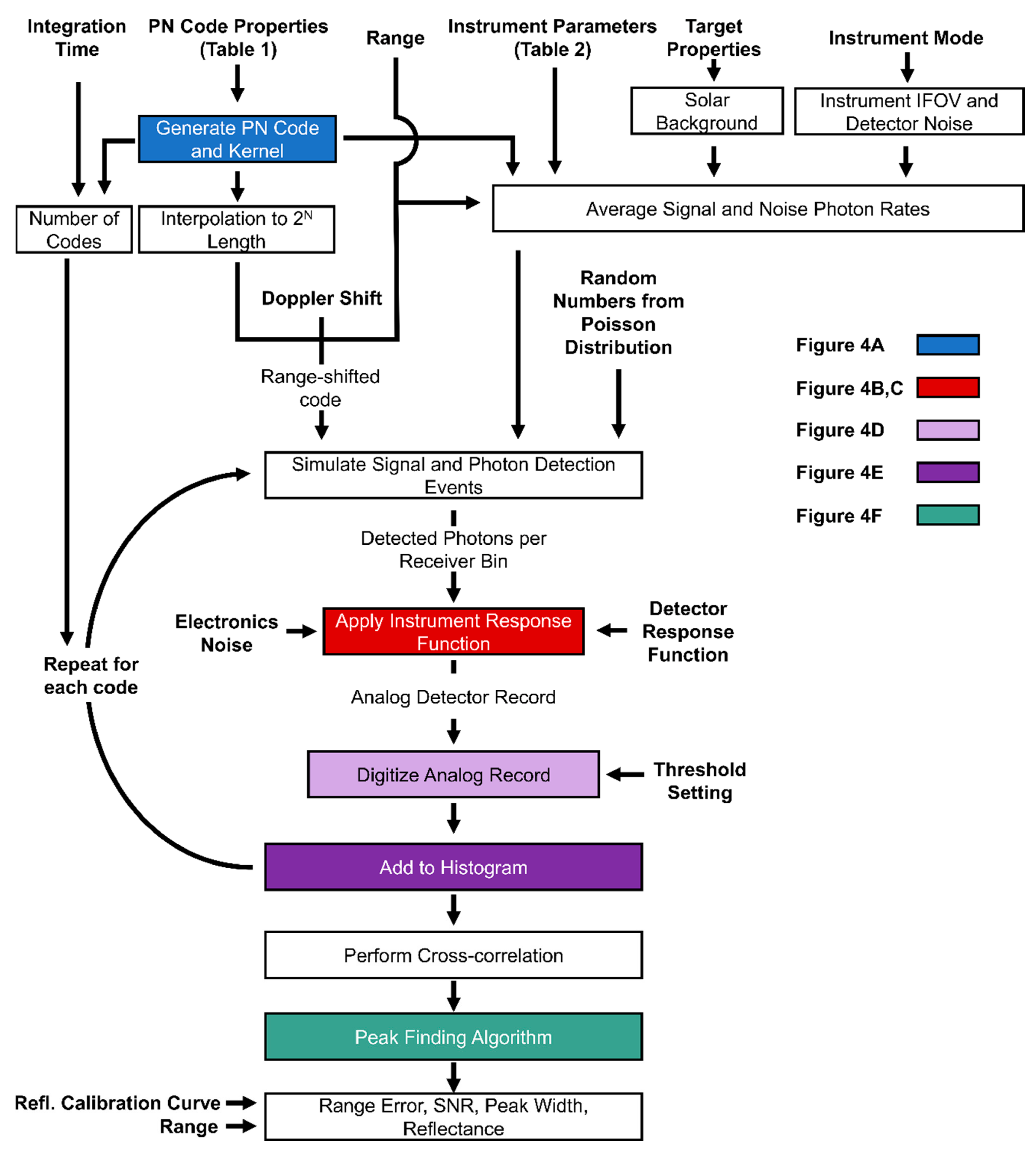
We constructed a numerical simulator to predict the ranging and surface reflectance performance of SALi for some expected conditions for a small-body mission. A flowchart of simulation stages is shown in Figure 3, and the simulation instrument and target parameters are summarized in Table 2.
First, the simulator generated the PN code and kernel using the parameters from Table 1 (Figure 4A). We then selected one of two instrument modes: long-range Reconnaissance mode, in which the digitized, accumulated signals from all 16 detector channels are summed prior to cross-correlation and the lidar acts as a laser range finder, and Mapping mode, where each detector channel is processed separately in series resulting in a swath-mapping lidar. The two modes are treated separately in the simulation based on their signal and noise levels and instantaneous fields of view (IFOVs).
2.4.2. Simulating Doppler Shift
Any line-of-sight velocity between the lidar and the target surface will induce a Doppler shift (i.e., a frequency change) in rate of the received PN code. Since the PN receiver accumulates signal over milliseconds or seconds for a single measurement, the Doppler shift can cause changes in the correlation. For small body missions the line-of-sight velocity of the spacecraft with respect to the target bod varies from centimeters to meters per second. In the performance simulation, Doppler shift is applied as a small additional range offset on a per-code basis.
For each transmitted PN code, the target range was used to precompute the time of flight. The received code and kernel were then resampled to 216 length to match the FPGA implementation. We used the selected instrument mode, range, integration time, and instrument and target characteristics given in Table 2 to determine the signal and noise photon detection rates.
2.4.3. Simulation of the Detected Signal and Noise Events
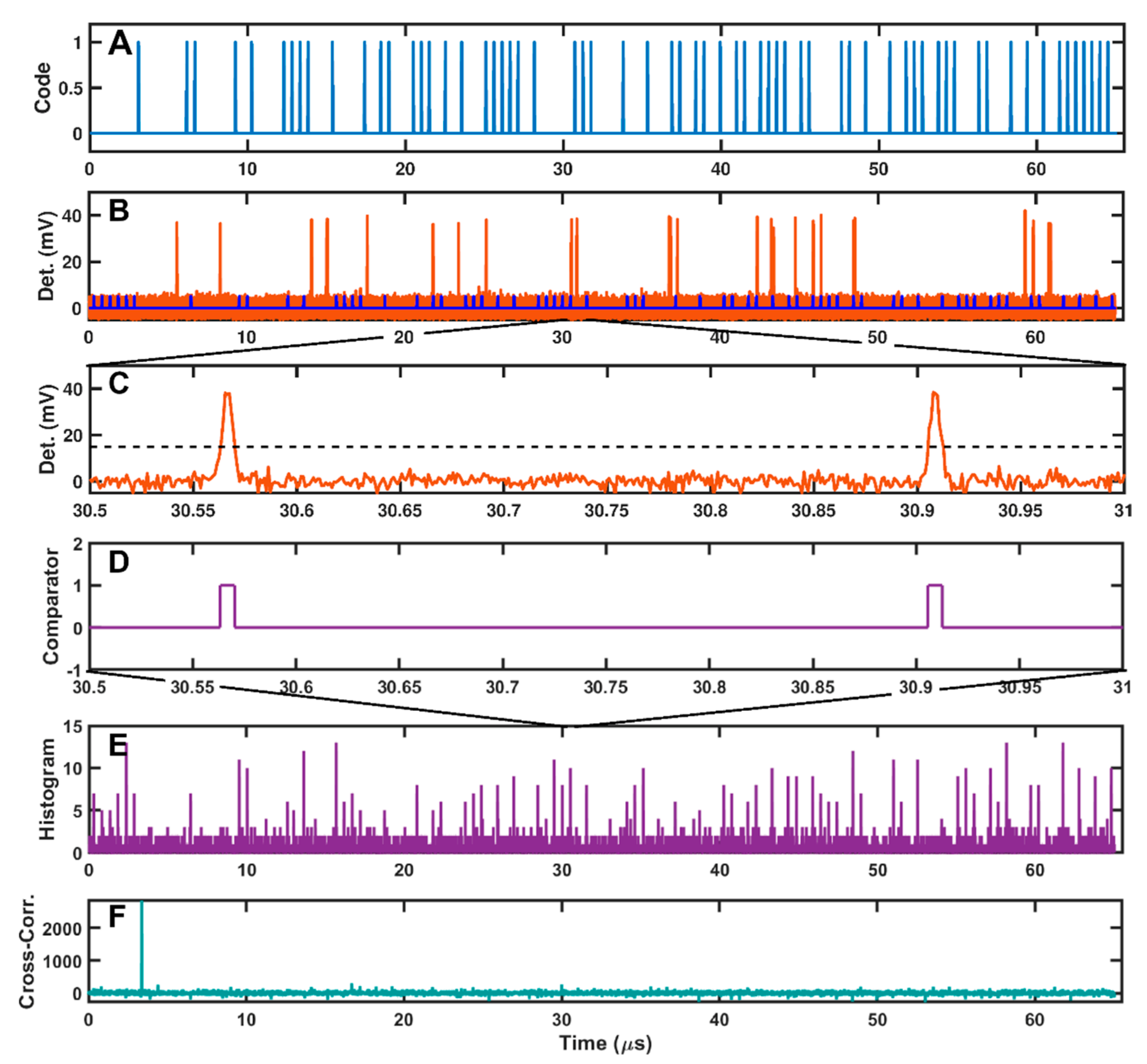
To determine if any photons were detected in each receiver time bin, the simulator calculates the incident signal photon rate and solar background photon rates based on the parameters in Table 2 and the lidar equation [29]. The photon detection process was modeled via the generation of random numbers from a Poisson distribution with mean values equal to the total photon events (signal photons and noise photons) for each receiver time bin. In general, speckle noise contributions from a rough target surface can degrade the lidar measurement and modify the signal detection process from following Poisson statistics to one described by a negative binomial distribution [30]. However, PN-code lidars accumulate tens to hundreds of thousands of pulses during the integration time, which makes speckle noise negligible compared to other noise sources. In addition, the laser linewidth from the fiber amplifier results in a high ratio of laser pulse duration to coherence time, which further reduces speckle effects [31].
Since the SALi HgCdTe APD is operated in linear photon-counting mode, each detected photon is modeled as a Gaussian shaped pulse with a random amplitude from a normal distribution with a mean of 30 mV and a standard deviation of 3 mV with a FWHM pulse width of 6 ns [32]. This was implemented by convolving the received photon events (delta functions) with the instrument response function given by the parameters above (Figure 4B,C). Figure 4B shows a representative analog signal in red and the range-shifted PN code in blue. Peaks in the red signal that align with peaks in the blue signal correspond to signal photon detection while the other red peaks correspond to detection of a noise photon. The detector’s electronic noise was modelled by adding zero-mean, 2-mV standard deviation Gaussian noise to each sample of the entire received code.
The digitizer stage converts the simulated analog detector waveform to a digital waveform. Ideally, the analog output from each channel would be sampled with a multi-bit analog to digital converter (ADC). However, the electrical power required for the ADCs for all pixels significantly increases the instrument’s electrical power. Here, as in the SALi design, we used a comparator as a one-bit digitizer (Figure 4D). Implementing the comparator approach as opposed to an 8-bit digitization approach saved ~8 W of power.
Due to the low-noise conditions and the single-photon performance of the HgCdTe APD array used here the range measurement performance was not sensitive to the comparator threshold for settings between 10 and 20 mV. For these simulations, the comparator threshold was maintained at 15 mV. Each code was then passed through this comparator to determine the binary value for each receiver bin. Each digitized code was then added to a histogram (Figure 4E), and the process was repeated starting with the next received PN code. Once the number of codes prescribed by the integration time was reached, we performed a cross-correlation in frequency space of the histogram results with the PN kernel (Figure 4F). Finally, the SNR, peak centroid, peak width, and range error were calculated from the correlation using the same methods as the FPGA implementation, though using floating point representation.
2.5. Bennu Orbit Simulation
We simulated the SALi PN code ranging approach on a relevant small body by extracting the surface elevation data of asteroid 101955 Bennu based on the OLA v20 shape model [33] using The Small Body Mapping Tool [34]. We chose 101955 Bennu due to the roughness of the surface and the availability of shape models with resolution finer than that of the 60-cm diameter SALi footprint from a nominal 10-km mapping orbit.
The track we extracted for the simulation is shown in Figure 5. We isolated the elevation for each shape model plate along the track and linearly interpolated the data to a uniform spacing (7 cm) along track. We then calculated the SALi footprint of a single pixel for each 10 ms measurement for a ground speed of 70 cm/s. Each footprint contained 9 interpolated elevation values based on the 10 km orbit altitude, which was assumed to be constant over the simulation. For each code length in each 10 ms measurement a time-of-flight was determined from a random sampling of the interpolated elevation values within the footprint. This introduced the effects of roughness within the laser footprint into the simulation. Because of the high measurement rate and low ground speed the footprints overlapped significantly. We decimated the measurement rate to 10 Hz but kept the measurement integration time at 10 ms to reduce the computation time while maintaining a footprint spacing equal to the interpolated ground track spacing. From this point the simulation was run exactly as described in Section 2.3. The surface reflectance was set to 0.04 based on OSIRIS-REx MapCam data [35,36] and the surface was assumed to be uniformly sunlit (the worst case for solar background noise).
2.6. Reflectance Measurement
To calculate the target reflectance, we use the peak amplitude of the cross-correlation to approximate the number of detected signal photons over the integration time. However, two effects complicate the reflectance measurement and must be addressed to avoid bias. First, a consequence of the finite detector response time and comparator threshold is that each detected photon can cause multiple adjacent 1’s in the histogram (Figure 6A). The exact number of 1s that are recorded on a photon-by-photon basis is non-deterministic and depends on the detector analog amplitude for each photon and the setting of the comparator threshold. Without correction this “comparator bias” leads to a positive bias in the surface reflectance measurement. Second, the comparator is unable to discriminate cases in which more than one photon reaches the detector within the detector response time (i.e., overlapping photons). In this case, the analog peak amplitude increases but the width of the detector response may not significantly change. Fewer than twice as many receiver bins are above the threshold compared to a single-photon event leading to a non-linear, negative detected pulse width bias in the reflectance measurement (Figure 6B).
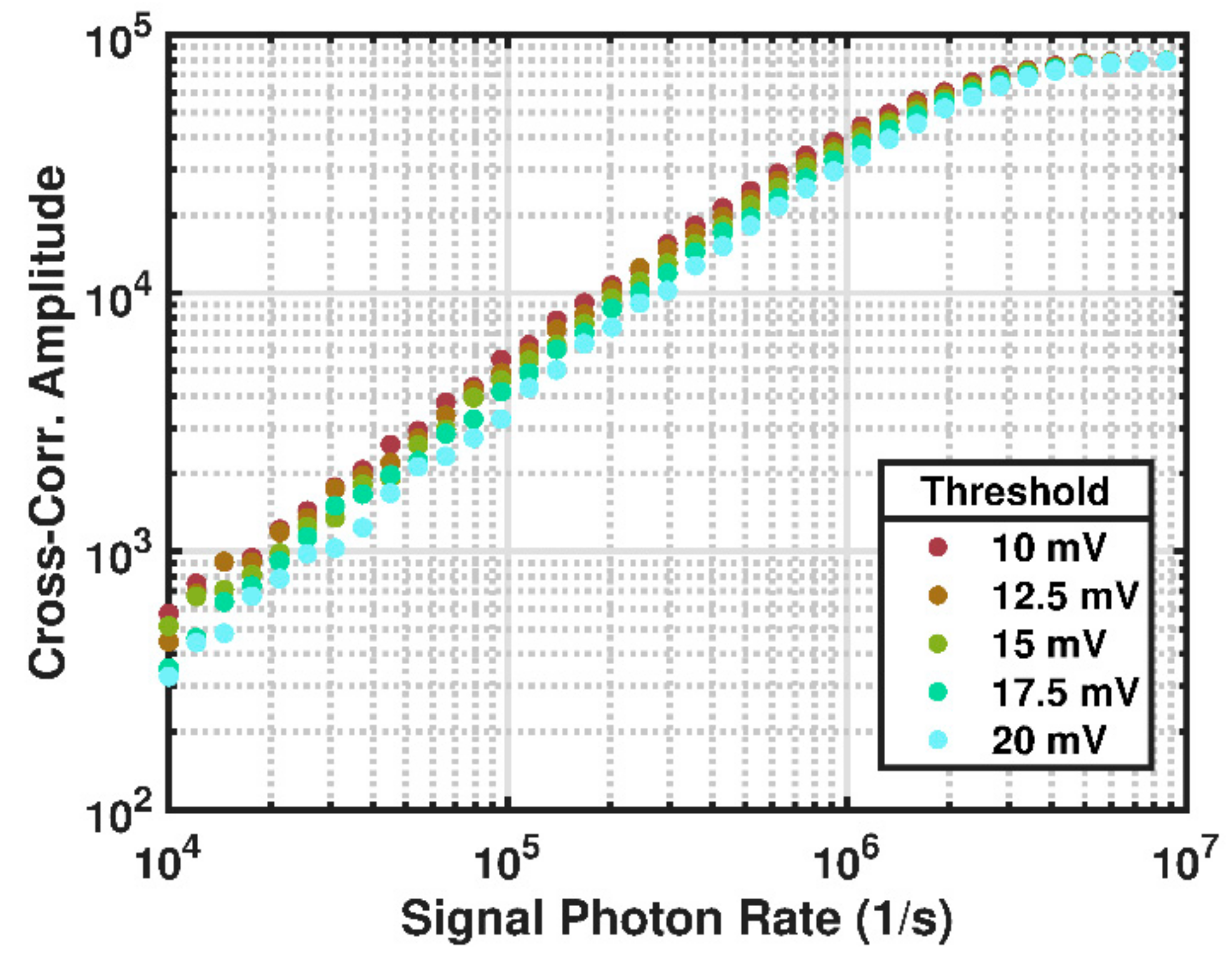
We designed a method to overcome these issues. Our method involves using laser power control with precomputed calibration curves that relate the cross-correlation amplitude to the signal photon rate. Laser power control is used to maintain a linear response of the cross-correlation amplitude to the signal photon rate. We ran a series of performance simulations to generate calibration curves of the cross-correlation amplitude as a function of input signal level (i.e., signal photon rate). These calibration curves are shown in Figure 7. The onset of non-linearity occurs around 1 × 10⁶ photons/s and eventually saturates, at which point the technique is no longer sensitive to surface reflectance. Our plan for the SALi lidar includes generating these calibration curves during hardware testing and implementing them as a look-up table in FPGA memory. The laser power is then adjusted via feedback from the cross-correlation results to keep the signal photon rate within the linear regime.
3. Results
3.1. Simulated PN Code Lidar Performance
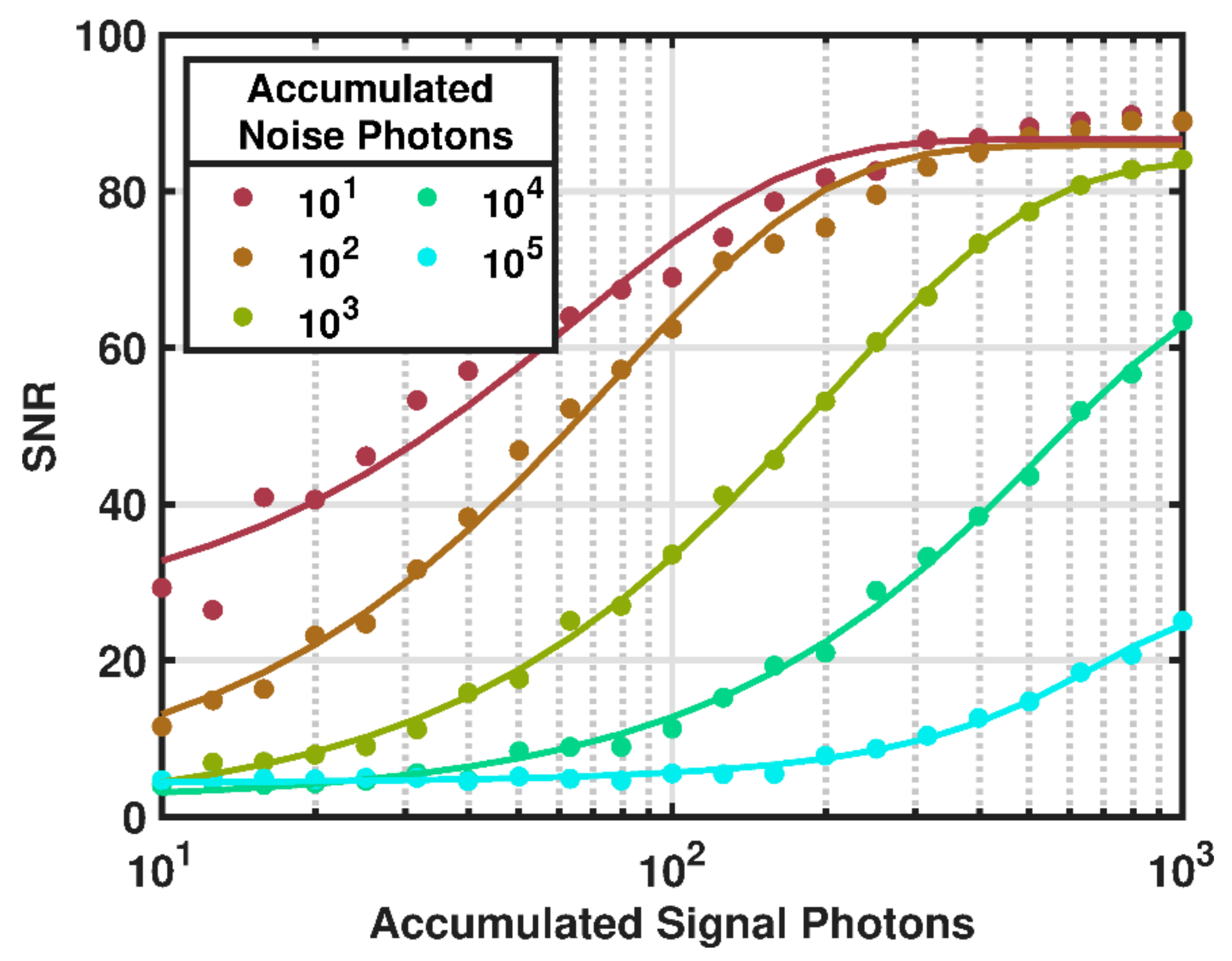
We first show simulation results of the SNR and range error over a range of accumulated signal and noise photons (Figure 8). In this case, the noise photon count includes detector dark noise, electronics noise, and solar background photons accumulated over the integration time, as described in Section 2.4.3. The signal photon count is similarly accumulated over the integration time.
Figure 8 shows the SNR as simulated over a range of signal and noise photon accumulations. The jaggedness of the results is due to the simulation photon detection process drawing randomly from a Poisson distribution, leading to small variations in performance at similar signal and noise levels. As the number of signal photons increases, the relative number of noise photons that can be accommodated while maintaining a high probability of detection also increases. The results show a PN code lidar achieves high SNR even under noise count levels that are 20 to 100 times higher than the signal photon count. Previous performance studies of pseudo-random code lidars have demonstrated this characteristic [38].
The PN code performance simulations numerically captured the complex correlation processing steps and quickly allow instrument element trade studies to be performed. A PN code lidar can be designed from scratch using known laser and detector parameters and an orbit simulation run to determine if the proposed instrument will likely meet the measurement requirements.
3.2. Simulated SALi Performance
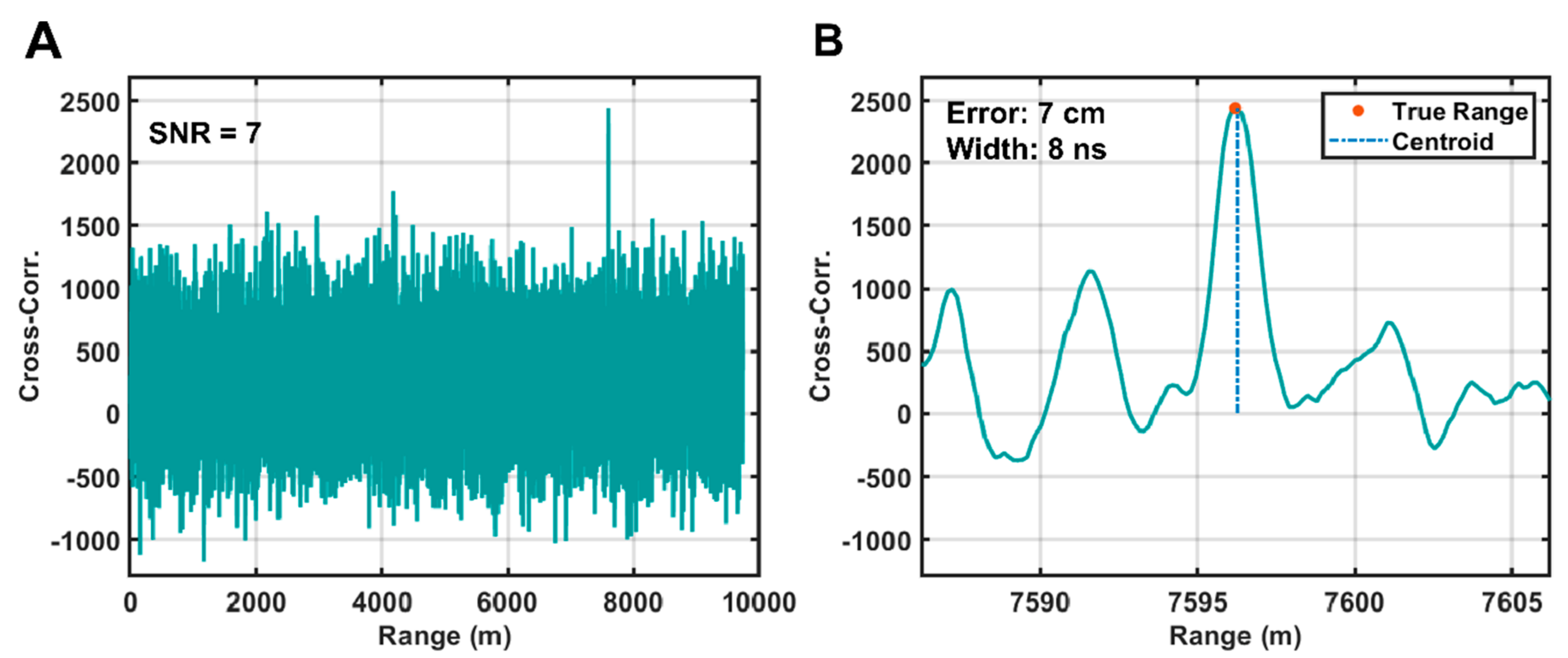
The results of the SALi performance simulations described in Section 2.4 are shown in Figure 9 and Figure 10 when operating Reconnaissance mode and Figure 11 and Figure 12 for the Mapping mode. For simplicity, all simulation results shown in Figure 9 through Figure 12 are for a flat target surface and zero-velocity conditions. Surface slopes and roughness within the laser footprint will increase the reflected pulse widths and increase the range errors shown in the figures. A representative cross-correlation simulation result for Reconnaissance mode is shown in Figure 9. The simulation conditions were a sunlit target at 300 km distance and a 2.5-s integration time. The peak of the cross-correlation resembles a Gaussian peak rather than a triangle function due to the convolution with the detector’s response. For the Reconnaissance mode, several competing effects modified the performance when compared to the Mapping mode. First, in this mode the signals from all 16 detector pixels are summed prior to digitization, which increases the signal photon rate. However, the detector’s dark noise from all pixels must be summed as well, and the longer integration time leads to an increase in solar background photons. The results show the ambiguous range is still correctly identified at 300 km with an error of 7 cm and the pulse width matches that expected from theory.
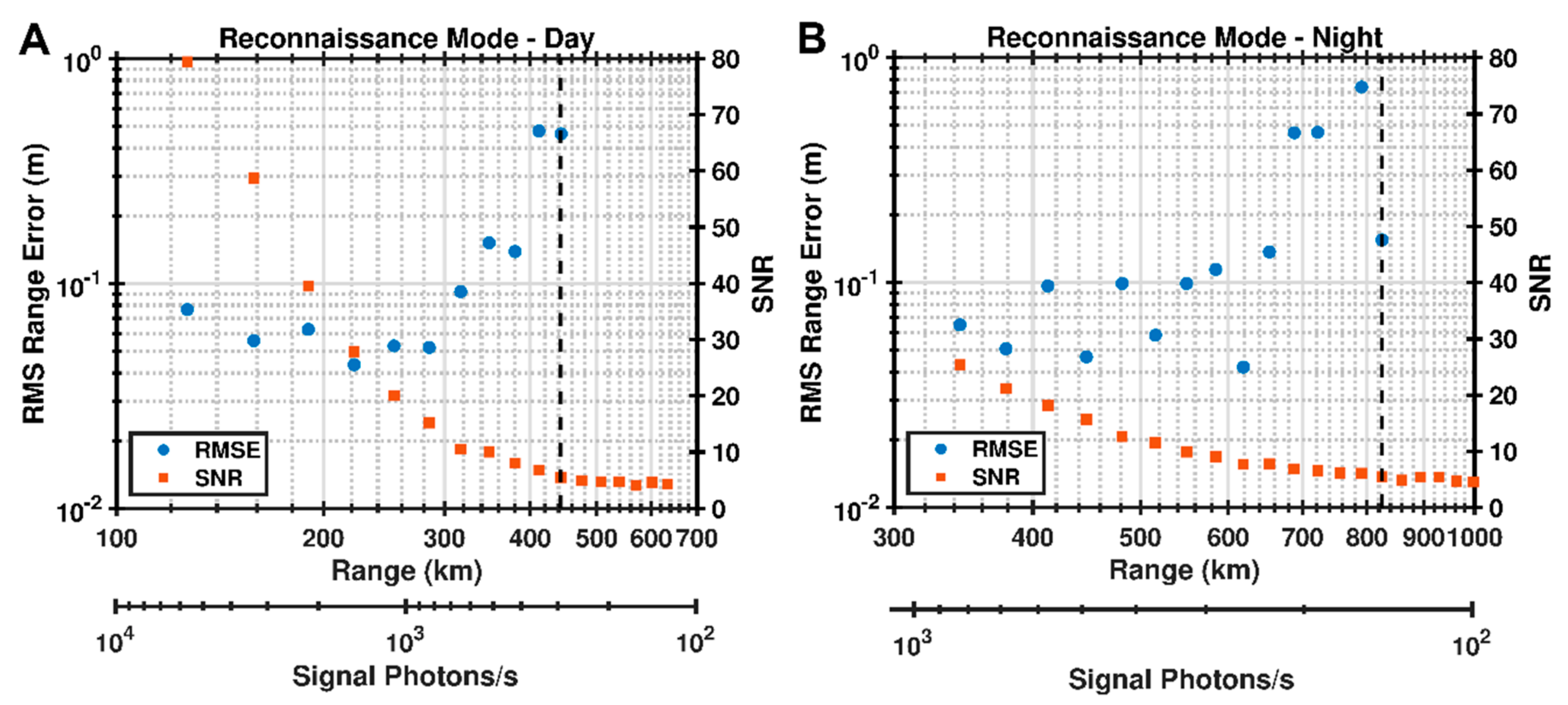
Figure 10 shows the simulation results for Reconnaissance mode for a 10-s integration time under sunlit conditions and shadowed conditions. We define a maximum achievable range as the highest tested range for which probability of detection was greater than 80% of the simulations yielding an accurate range. Ranging errors above one meter indicated false detection, which generally corresponded to SNR values of ~6 or below. The maximum ranges as defined above were 440 km and 820 km for day and night, respectively. For the flat target surface used in the simulation, the average RMS errors below 400 km were 8 cm and 6 cm for day and night, respectively.
Figure 11 shows a representative cross-correlation result taken under sunlit conditions in Mapping mode from a 50 km orbit with a 0.1-s integration time. The ranging error for this trial was 4 cm, which is within the theoretical root mean square (RMS) error of 5.8 cm calculated based on the signal to noise ratio, sampling rate, and laser pulse width [39]. The width of the cross-correlation peak is 9 ns, the precision of which is limited by the FPGA centroiding method described above but approximates the theoretical width of 8.4 ns from the convolution of the output laser pulse with the detector response function. The performance as a function of range for the Mapping mode is show in Figure 12 for both sunlit (day) and shadowed (night) target conditions.
For the 50 km range of Mapping mode, the simulation results in Figure 12 show an average RMS ranging errors of 4 cm and 5 cm for sunlit and shadowed conditions, respectively. The maximum range was measured as 110 km under sunlit conditions and 130 km with the target in shadow. The results from the SALi simulations showed its capabilities are consistent with those given in our instrument overview [11]. The Mapping mode performance exhibited a SNR near 25 and a range precision below 6 cm. This suggests that the integration time can be shortened to 0.01 s to map the target body more densely, or the laser pulse energy can be lowered to reduce overall instrument power in this mode.
3.3. Doppler Effect
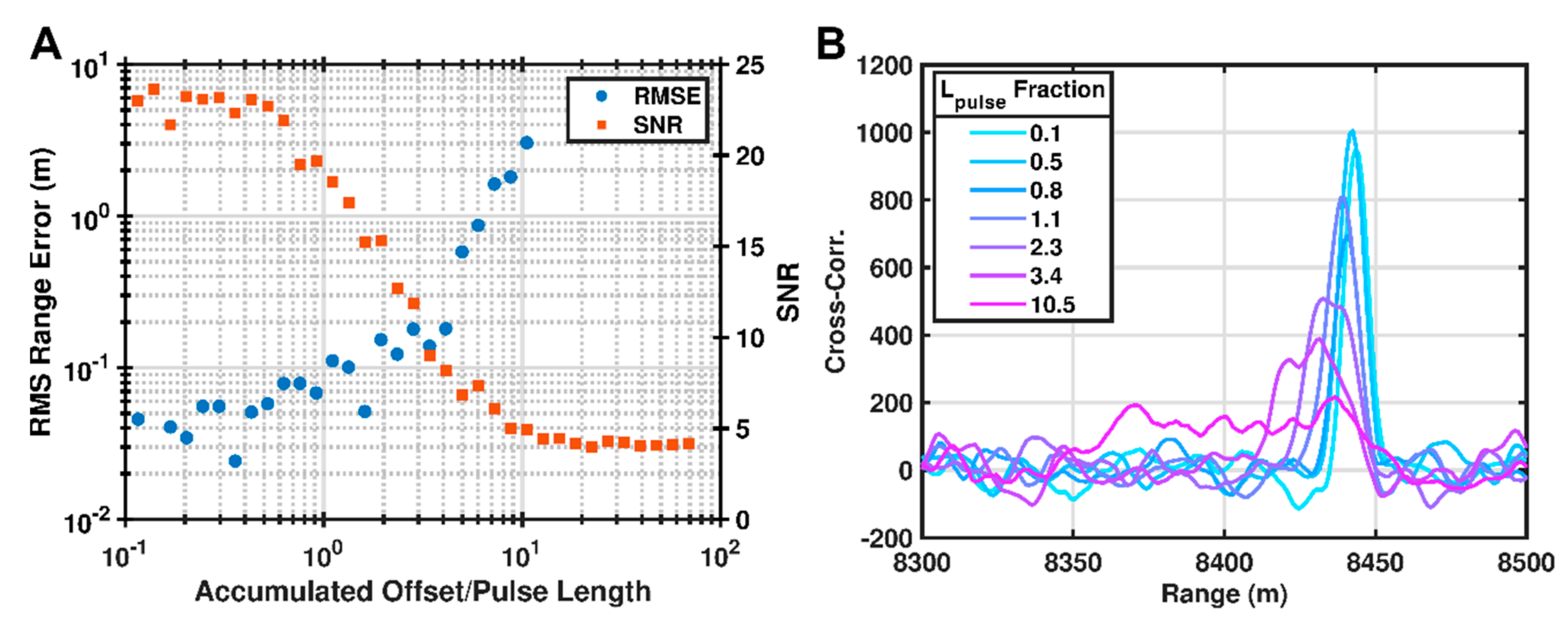
The effects of accumulated Doppler shift on the PN ranging performance are shown in Figure 13. The results shown are for a Mapping mode simulation with accumulated Doppler shift (in units of fractional pulse length) between 0.1 and 70. This range corresponds to uncompensated spacecraft velocities (due to orbit prediction errors during data acquisition and due to unknown topography roughness) of 11 m/s to 8000 m/s for a 10-ms integration (Mapping mode) or 0.01 m/s to 8 m/s for a 10-s integration (Reconnaissance mode). For this simulation, the Doppler shift was assumed to be negative, that is, the spacecraft was assumed to be moving towards the target body. The Doppler effect spreads the peak of the cross-correlation and reduces the amplitude with respect to the baseline, thus reducing the SNR. When the accumulated Doppler shift (i.e., the distance covered by the spacecraft during the integration time) is less than half the fractional pulse width, there is no significant change in performance. Between 0.5 and 10 times the pulse length the performance degrades until the probability of detection becomes <50% above 10 times the pulse length. Thus, for Mapping mode at 100 Hz the Doppler compensation does not affect the measurement at uncompensated spacecraft velocities below ~75 m/s. This velocity is large in relation to typical spacecraft orbits around small bodies but should be considered when designing slews or other maneuvers that may lead to large range changes over the measurement time. For Reconnaissance mode, however, the Doppler shift must be pre-compensated by adjusting the receiver clock rate to better than 7.5 cm/s for a 10-s integration and 75 cm/s for a 1-s integration to avoid a reduction in ranging performance.
For SALi, the Doppler effect is negligible in Mapping mode but may affect Reconnaissance mode performance unless corrected for by modifying the receiver clock rate in real time. Residual range rate uncertainty for recent small body missions is on the order of 5 to 10 cm/s [11], which brackets the required range rate correction level (7 cm/s) for a 10-s integration in Reconnaissance mode. For ranging to larger planetary bodies (such as the Moon or Ceres) with accompanying large elevation changes and high (100s of m/s to km/s) ground speeds the Doppler effect may significantly affect performance. Depending on the spacecraft orbit and target conditions, this sets constraints on the integration time, and thus the operational range of the lidar under Doppler conditions. However, this effect can be ameliorated by increasing the laser power to reduce the required integration time. For example, if the residual range rate uncertainty requires the integration time be reduced by a factor of 2 to meet the required range precision, the laser power must increase by a factor of . The 2-W SALi design is not presently limited in laser power. A 4-W fiber amplifier system was flown as part of the Optical Communications and Sensors Demonstration (OCSD) program [40]. The laser pulse width can also be extended such that the difference in correlation peak width between the stationary and Doppler cases (Figure 13B) is reduced. To first order, the ranging precision scales linearly with the laser pulse duration [29].
3.4. Simulation Results for a Bennu Orbit
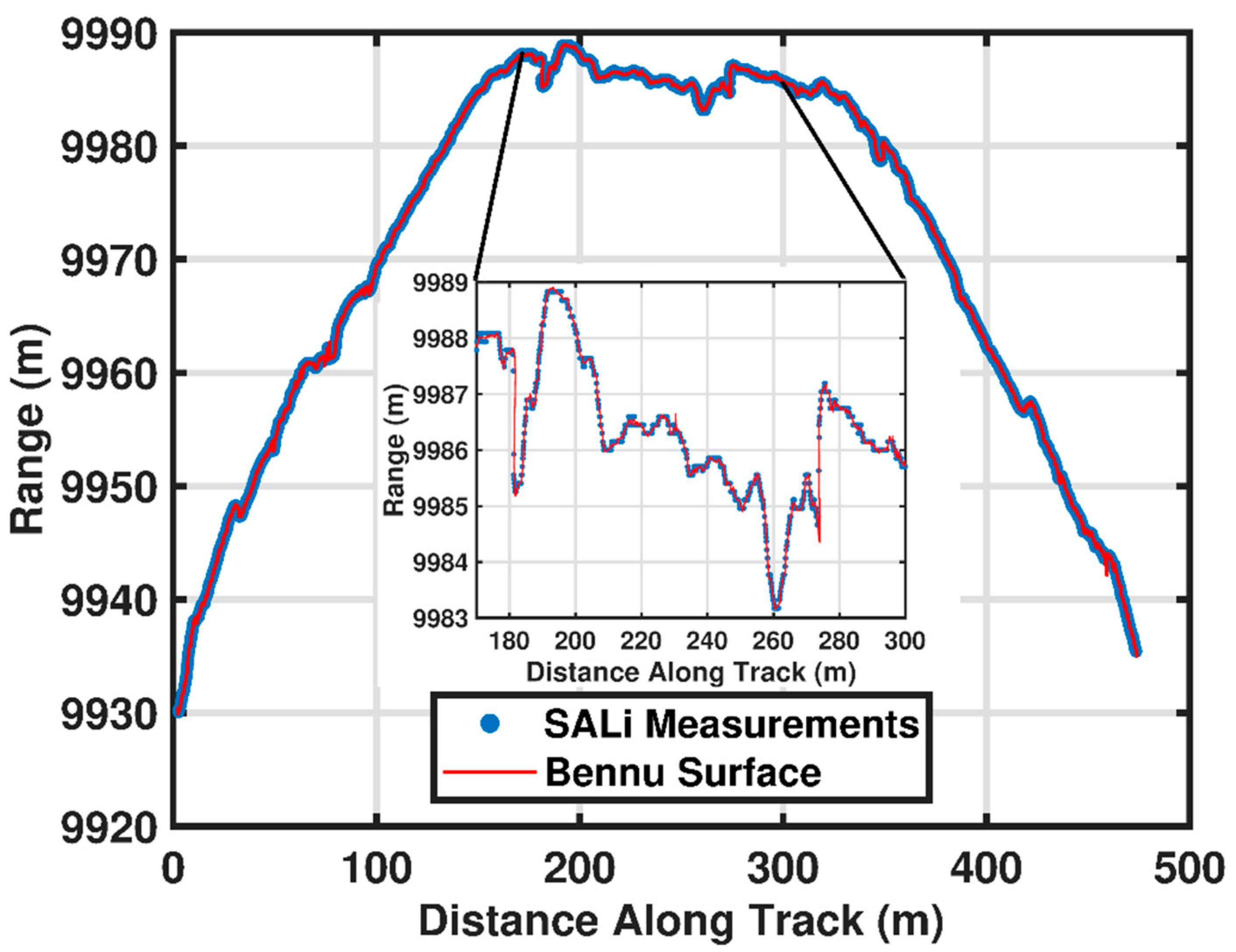
The results of the 101955 Bennu simulation (see Section 2.5) are shown in Figure 14. The ranges (as calculated from the 10-km spacecraft altitude minus the surface elevation with the laser pointed at nadir) were accurately measured over the entire track, including in most regions of sharp elevation changes, as shown in the inset of Figure 14. Positive and negative slopes up to 60 degrees over a 60 cm baseline were measured with residual errors under 10 cm. This includes the effect of roughness within the laser footprint as described in Section 2.5.
Range residuals for the Bennu simulation are shown in Figure 15 as a function of distance along the ground track. In total there were 6730 independent measurements each comprising 154 code-lengths. The mean of the residuals was −0.007 cm, and the standard deviation was 5 cm, in good agreement with the standard deviations from the Mapping mode simulation results shown in Figure 12.
There were several regions of the track where residuals were larger, one of which is shown in Figure 16. These residuals were the result of the sheer faces of boulders or overhangs within the footprint of SALi (gold line in Figure 16). The lidar beam could not sample the surface beneath the overhangs based on the nadir-pointing geometry of the simulation. There were also cases where the footprint of the lidar spanned a steep slope or cliff, and the centroid process resulted in a mean range that was between the two elevation extremes. However, these cases were easily distinguishable by tracking the width of the cross-correlation peak, which is plotted in Figure 16 for the same region. In practice, regions of high slope such as these would require repeat mapping, potentially at lower altitude to shrink the lidar footprint, and using either off-nadir pointing control implemented as part of the instrument (as OLA did at Bennu) or by slewing the spacecraft.
3.5. Reflectance Measurement
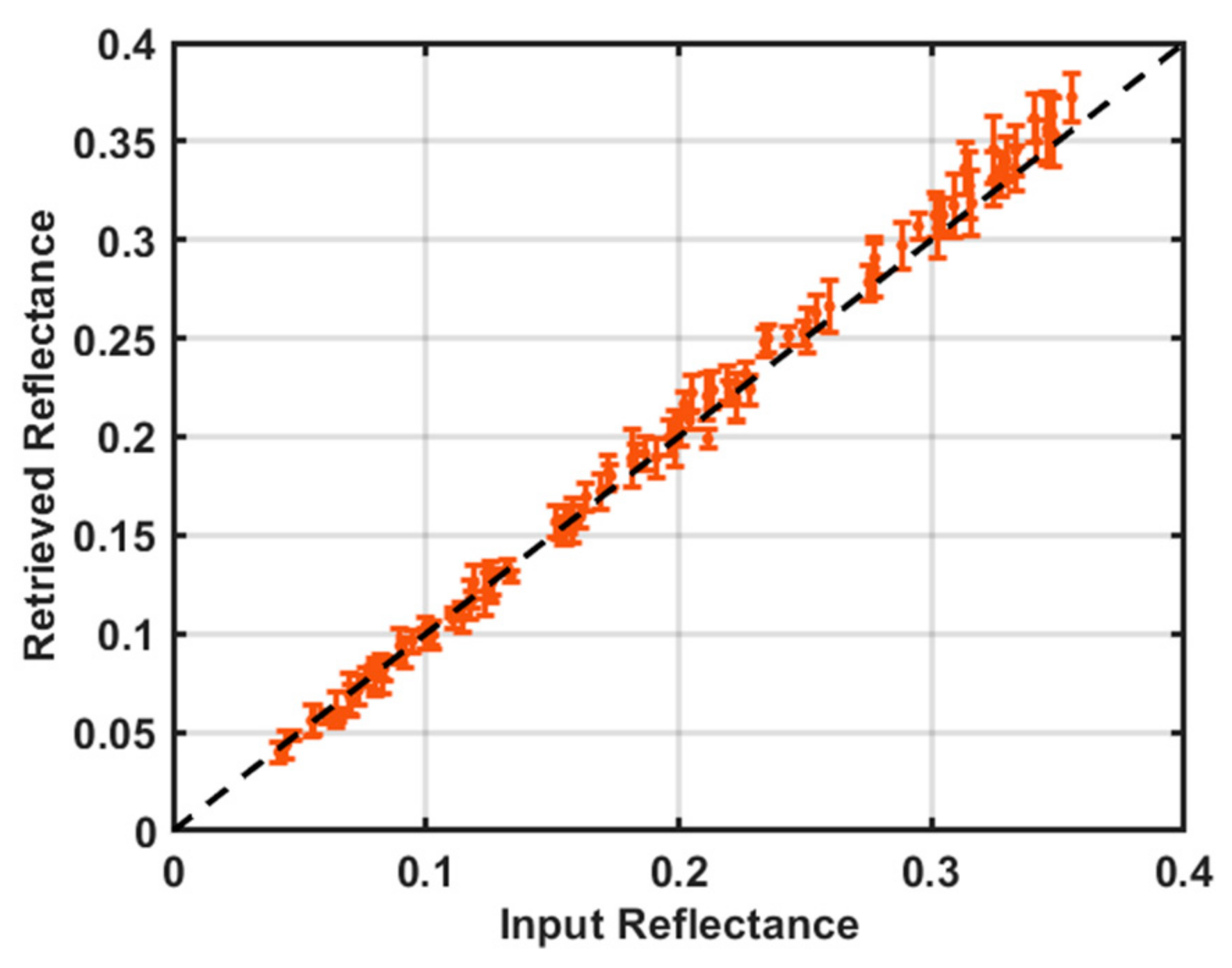
The surface reflectance of small bodies can vary considerably. We tested the reflectance algorithm in Mapping mode (20-km altitude, 100 Hz rate) by using randomized surface reflectance conditions that varied from 4% to 36%. This range was selected using the reflectance of 101955 Bennu (0.041 at 1550 nm [35,36]) and 25143 Itokawa (0.36 at 1550 nm [41]) as end-members. The laser power in the simulation was adjusted to 0.5 W to maintain cross-correlation amplitude in the linear regime. The measured cross-correlation amplitudes were converted to signal photon rate using the calibration curves in Figure 7. The results are shown in Figure 17. Over the tested reflectance range, the measurements exhibited an average bias of 1% of the input reflectance value and a 1-σ precision of 3% of the input reflectance value. The small positive bias is likely due to the counting of background noise photons during laser pulse periods that is not accounted for in the calibration curves in Figure 6. This bias is not inherent to the measurement and can be included in the calibration for known target illumination conditions.
3.6. Data Processing Time with a XCKU060 FPGA
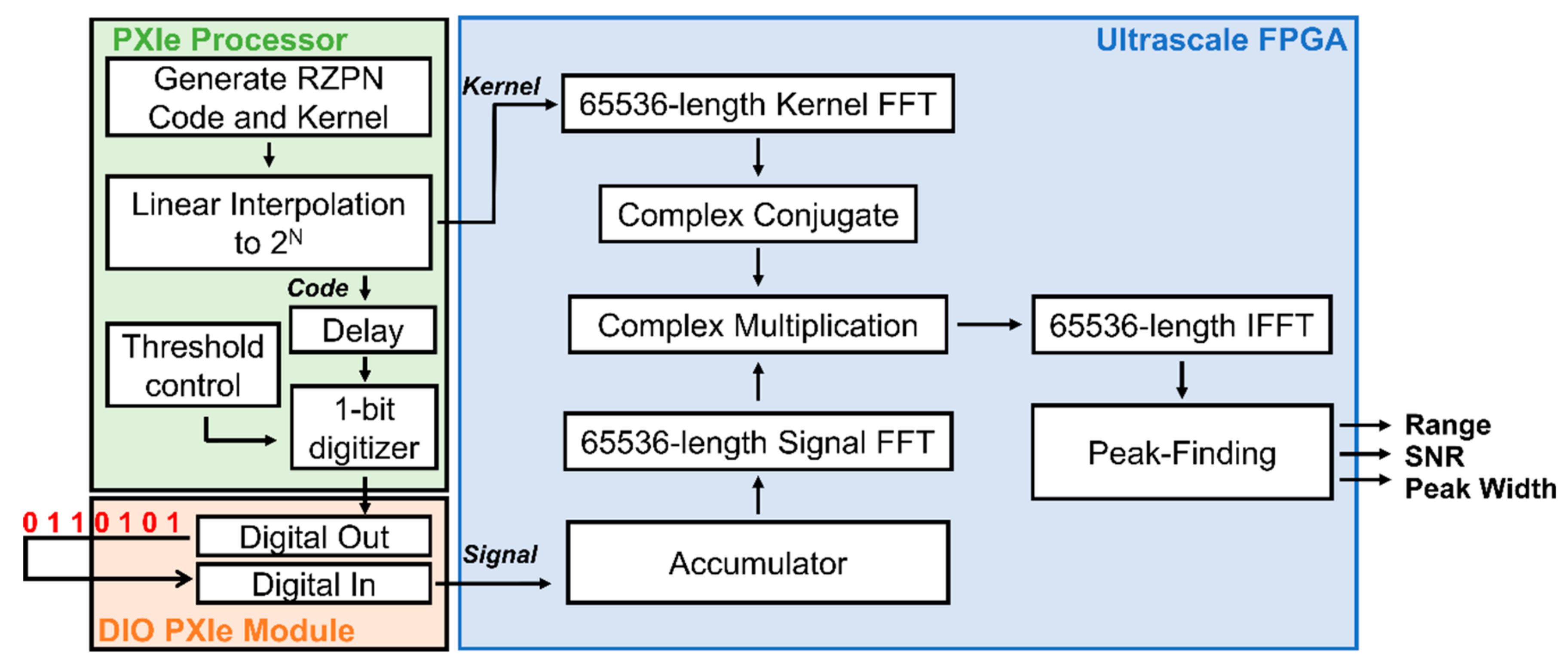
The PN code lidar receiver requires significant onboard digital signal processing to implement ranging in real-time. To determine the required resources to process the PN code for real-time ranging at a desired 16-channel measurement rate of 100 Hz, we implemented the FFT correlation algorithm of the PN code and kernel from Section 2.1 on a National Instruments (NI) PXIe FPGA system. We ran benchmark and validation tests to determine the processing throughput and latency using a Xilinx KU060 FPGA [42]. Our choice of an XCKU060 FPGA was based on our initial estimate of the required resources as well as its ongoing path to spaceflight qualification [43,44]. This is the same FPGA chosen for the prototype version of SALi [11].
A block diagram of the PN processing breadboard for the FPGA is shown in Figure 18. The PN code and kernel were generated on an NI PXIe processer with linear feedback shift registers. The kernel and code were then linearly interpolated to 216 and the code was circularly shifted simulating a time-of-flight. The code was then passed through a comparator to simulate the 1-bit digitizer present in the SALi design. The delayed code was passed to a NI digital IO module and transmitted and received in a loopback fashion. The received digital code was accumulated into onboard FPGA memory (10-bit depth, 65,536 length) for the requested number of code lengths before being transmitted to the correlation stage. The cross-correlation processes were compiled at the highest clock rate possible (200 MHz) to determine the fastest single-channel measurement rate (latency and throughput) possible under the hardware constraints.
Each FPGA clock cycle, single samples of the time-shifted, accumulated PN code (hereafter referred to as the signal) and kernel were read from block random access memory (BRAM) and passed to the inputs of separate Xilinx LogiCORE IP FFT cores (v.9.0). The FFT core is a reusable code block that implements the Cooley-Tukey algorithm to calculate the discrete Fourier transform of the input signal. The FFT cores were parametrized to run in pipelined mode (decimation-in-frequency method with radix-4 butterflies) for continuous data processing. The signal was presented to the FFT cores as fixed-point, signed 10-bit integers, and all integer bit growth was negated via scaling at each radix stage, which dramatically reduced BRAM usage. Careful design of the scaling at each FFT and IFFT stage was performed to minimize truncation/roundoff error [45,46]. Here, we chose a scaling implementation of 8 bits of scaling distributed through the stages in the signal FFT, kernel FFT, and inverse FFT (IFFT). To avoid overflow and minimize roundoff error, the scaling implementation should be optimized under expected signal levels. The scaling will be re-examined during SALi prototype testing but is already accounted for in the processing resource usage.
Next, the Fourier transform of the signal and the complex conjugate of the kernel transform were passed into a complex multiplier, the result of which was passed to an IFFT core. The parameterization of the IFFT core was the same as the forward FFT cores except for the input and output bit depth and the bit scaling at each radix stage. The output of the IFFT is the scaled result of the cross-correlation, ideally with a global maximum at the index corresponding to the lag of the PN code with respect to the kernel (i.e., the unambiguous range). We implemented a peak search algorithm that is compatible with the point-by-point output of the IFFT node. The algorithm tracks the value and index of the current highest value in the cross-correlation by comparing the value at each new index with the present highest value. The highest value of the cross-correlation, rather than the peak area, is sufficient in determining the signal strength as correlating the signal with the kernel is akin to integration. The threshold for the rising and falling edges were set to half the peak value. The peak width was calculated using the rising-edge and falling-edge threshold crossings of the cross-correlation. The peak centroid was estimated by the falling edge minus half the peak width, which is valid for symmetric peaks [47]. Finally, the FPGA sent the cross-correlation peak value, width, and centroid index to the PXIe processor where it was written to file.
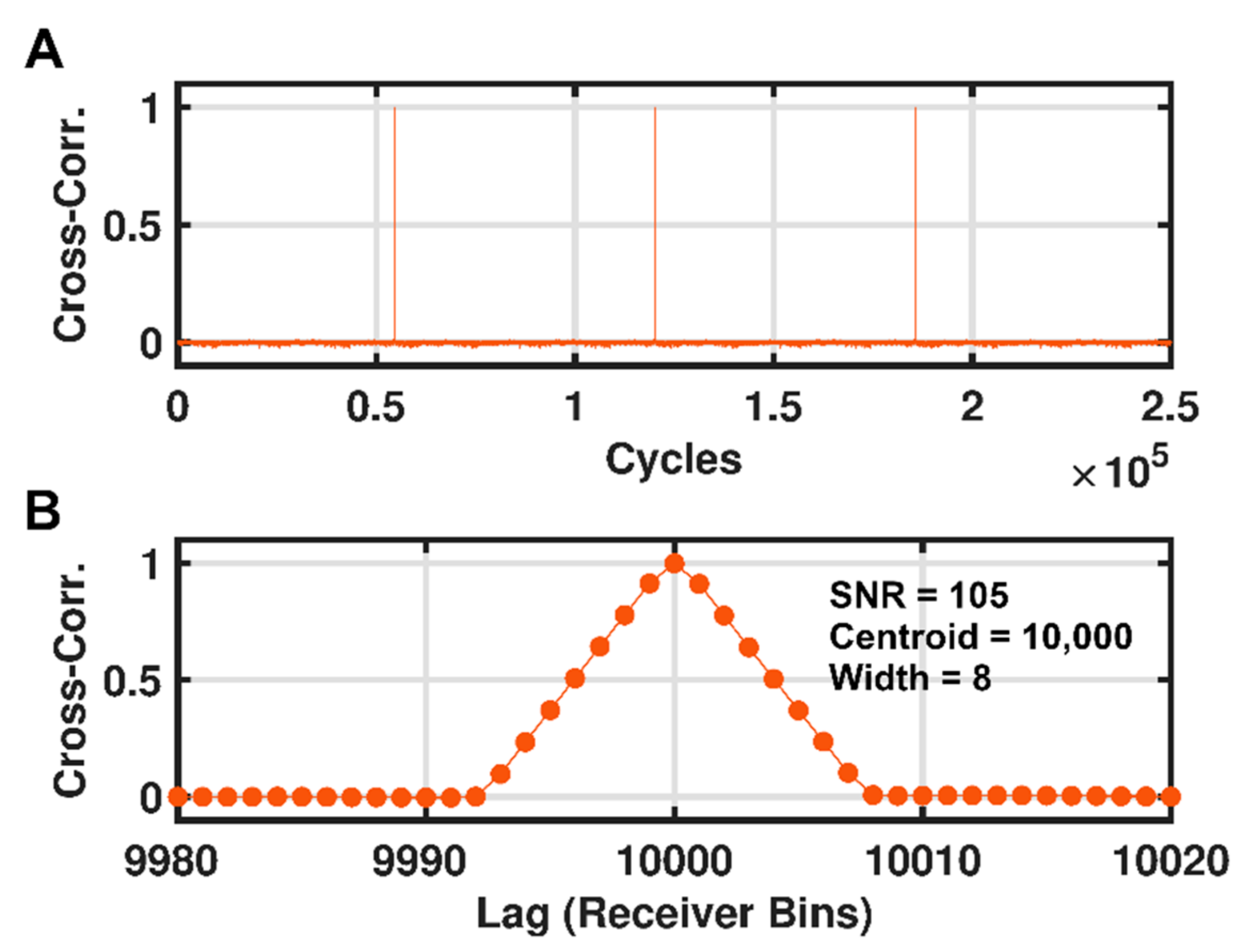
The performance figures of merit for the FPGA breadboard are the accuracy of the processing steps (e.g., range retrieval, SNR), the processing latency, and the throughput. Representative results of the FPGA implementation of the SALi processing pipeline are shown in Figure 19. The pipelined streaming architecture allows the FFT cores to load the next frame of data while processing or unloading the previous frame. This results in back-to-back correlation outputs with no dead-time between computations (Figure 19A) after an initial latency period upon startup. The pipelined streaming architecture results in the highest processing throughput but is also the most resource intensive. Each 65,536-length correlation is output in a point-by-point fashion (i.e., one value per clock cycle) at a clock rate of 200 MHz. For the experiment in Figure 19, a lag of 10,000 was set on the PXIe processor, and the accumulation was set for 500 code lengths prior to correlation.
Figure 19B shows the correlation peak, which occurred at the correct lag value (10,000), with a peak width equal to the pulse width (eight bins), and a SNR of 105. The slight reduction in SNR compared to Figure 2D was caused by the truncation/roundoff errors introduced during fixed-point FFT calculations. The roundoff error increased slightly as the number of accumulated codes decreased, with a SNR of 97 measured for 200 accumulated codes. The peak shape closely resembles the expected triangular function but with slight rounding near the peak and corners due to the linear interpolation and threshold process. Additional experiments verified the lag was accurately tracked over the entire code period. The FPGA resource usage of the XCKU060 based on the current SALi design is <10% for all resources except block RAM (77%) and IO (23%).
Other important signal processing characteristics are the processing latency and throughput. The processing latency is defined here as the time from the read-in of the first signal bin from the accumulator to the output of the centroid, width, and SNR of the cross-correlation. The measured latency was 1.07 ms for a single channel, which enables SALi to provide range information to the navigation scheme in real-time to support landing operations. The processing throughput is the number of correlations per second that can be performed assuming data is always present at the correlator input (i.e., regardless of signal integration time). The measured single-channel throughput was 3050 Hz. The PN code breadboard experiments were designed to test the processing algorithm and benchmark the latency and throughput, but the NI breadboard system can also form the core of a PN lidar with minimal modifications. The signal from the digital output can be used to drive a transmitter laser diode, while a detector and comparator can be connected to the digital input that feeds directly into the FPGA for correlation.
4. Conclusions
We have described simulation studies and the implementation of a real-time processing approach for an PN code lidar (SALi) for planetary missions to small bodies. SALi uses a return to zero PN code and is designed to operate as a mapping and survey lidar, with a single-beam Reconnaissance mode out to 400 km and a 16-pixel Mapping mode to 50 km. In addition, it can support descent and surface sampling by providing ranges at a 100 Hz measurement rate with 16 channels.
Simulations of the lidar performance quantified the anticipated performance. In the long-range Reconnaissance mode, SALi obtained accurate ranges to 440 km with a precision of 8 cm below 400 km. In Mapping mode, accurate ranges were retrieved up to 90 km in altitude with a ranging precision of 5 cm at altitudes of 50 km and lower. We also developed a reflectance algorithm using active laser control to determine the surface reflectance to a precision of 3% of the surface reflectance values from 4% to 36%. These simulations have also uncovered several relevant PN code design aspects that have not been previously described in detail. These include the binary aspect of the range error, the correlation acting as a low-pass filter, the FFT length considerations, the Doppler sensitivity limits, and the quantitative reflectance measurement method. Finally, the PN ranging algorithm was tested using simulated measurements of the surface of asteroid 101955 Bennu. The range residual standard deviation was 5 cm with a sub-mm bias.
The FFT-based processing algorithm implemented on a Xilinx Ultrascale FPGA performed the required cross-correlation range measurement at a maximum throughput of 3050 Hz with a latency of 1.07 ms for a single channel. Based on these results, the SALi PN code approach was shown to be feasible as a high-measurement-rate ranging and reflectance lidar well-suited for future missions to small bodies.
Author Contributions
Conceptualization, D.R.C., X.S. and J.B.A.; methodology, D.R.C.; software, D.R.C.; validation, D.R.C.; formal analysis, D.R.C., X.S., E.M. and J.B.A.; investigation, D.R.C.; writing—original draft preparation, D.R.C. and X.S.; writing—editing and revising, D.R.C., X.S., J.B.A. and E.M.; visualization, D.R.C.; project administration, X.S. All authors have read and agreed to the published version of the manuscript.
Funding
This research was funded by the NASA GSFC Internal Research and Development (IRAD) programs for Fiscal Years 2008, 2009, 2010, 2013, and 2014. It is currently funded by the NASA Science Mission Directorate (SMD) Maturation of Instrument Technologies for Solar System Exploration (MatISSE) program, Award 18-MatISSE18_0-0029.
Institutional Review Board Statement
Not Applicable.
Informed Consent Statement
Not Applicable.
Data Availability Statement
Publicly available datasets were analyzed in this study for the Bennu simulations. This data can be found here: http://sbmt.jhuapl.edu/Object-Template.php?obj=77. Additional Bennu shape model data can be found at the Planetary Data System Small Bodies Node: https://sbn.psi.edu/pds/resource/bennushape.html.
Acknowledgments
We thank Mark Storm and Jacob Hwang of Fibertek, Inc. for their participation in the SALi instrument development effort. We also thank Michael Albert, formally of Fibertek, Inc. for the initial optical and system design of SALi.
Conflicts of Interest
The authors declare no conflict of interest.
References
- Jewitt, D.; Haghighipour, N. Irregular Satellites of the Planets: Products of Capture in the Early Solar System. Annu. Rev. Astron. Astrophys. 2007, 45, 261–295. [Google Scholar] [CrossRef] [Green Version]
- Levison, H.F.; Bottke, W.F.; Gounelle, M.; Morbidelli, A.; Nesvorný, D.; Tsiganis, K. Contamination of the asteroid belt by primordial trans-Neptunian objects. Nature 2009, 460, 364–366. [Google Scholar] [CrossRef] [PubMed]
- Bottke, W.F.; Nesvorný, D.; Vokrouhlický, D.; Morbidelli, A. The irregular satellites: The most collisionally evolved populations in the solar system. Astron. J. 2010, 139, 994–1014. [Google Scholar] [CrossRef] [Green Version]
- Binzel, R.P.; DeMeo, F.E.; Turtelboom, E.V.; Bus, S.J.; Tokunaga, A.; Burbine, T.H.; Lantz, C.; Polishook, D.; Carry, B.; Morbidelli, A.; et al. Compositional distributions and evolutionary processes for the near-Earth object population: Results from the MIT-Hawaii Near-Earth Object Spectroscopic Survey (MITHNEOS). Icarus 2019, 324, 41–76. [Google Scholar] [CrossRef] [Green Version]
- Zuber, M.T.; Smith, D.E.; Cheng, A.F.; Cole, T.D. The NEAR laser ranging investigation. J. Geophys. Res. E Planets 1997, 102, 23761–23773. [Google Scholar] [CrossRef]
- Yoshimitsu, T.; Kawaguchi, J.; Hashimoto, T.; Kubota, T.; Uo, M.; Morita, H.; Shirakawa, K. Hayabusa-final autonomous descent and landing based on target marker tracking. Acta Astronaut. 2009, 65, 657–665. [Google Scholar] [CrossRef]
- Mizuno, T.; Kase, T.; Shiina, T.; Mita, M.; Namiki, N.; Senshu, H.; Yamada, R.; Noda, H.; Kunimori, H.; Hirata, N.; et al. Development of the Laser Altimeter (LIDAR) for Hayabusa2. Space Sci. Rev. 2017, 208, 33–47. [Google Scholar] [CrossRef]
- Daly, M.G.; Barnouin, O.S.; Dickinson, C.; Seabrook, J.; Johnson, C.L.; Cunningham, G.; Haltigin, T.; Gaudreau, D.; Brunet, C.; Aslam, I.; et al. The OSIRIS-REx Laser Altimeter (OLA) Investigation and Instrument. Space Sci. Rev. 2017, 212, 899–924. [Google Scholar] [CrossRef]
- Sornsin, B.A.; Short, B.W.; Bourbeau, T.; Dahlin, M. Global shutter solid state flash lidar for spacecraft navigation and docking applications. In Proceedings of SPIE, Proceedings of the Laser Radar Technology and Applications XXIV, Baltimore, MD, USA, 14–18 April 2019; p. 110050W. [Google Scholar]
- Smith, D.E.; Sun, X.; Mazarico, E.M.; Zuber, M.T. Asteroid Lidar for Topography, Mapping, and Landing. In Proceedings of the Lunar and Planetary Science Conference, The Woodlands, TX, USA, 18–22 March 2019; p. 1421. [Google Scholar]
- Sun, X.; Cremons, D.R.; Mazarico, E.; Yang, G.; Abshire, J.B.; Smith, D.E.; Zuber, M.T.; Storm, M.; Martin, N.; Hwang, J.; et al. Small All-range Lidar for Asteroid and Comet Core Missions. Sensors 2021, 21, 3081. [Google Scholar] [CrossRef]
- Macwilliams, F.J.; Sloane, N.J.A. Pseudo Random Sequences and Arrays. Proc. IEEE 1976, 64, 1715–1729. [Google Scholar] [CrossRef]
- Takeuchi, N.; Sugimoto, N.; Baba, H.; Sakurai, K. Random modulation cw lidar. Appl. Opt. 1983, 22, 1382–1386. [Google Scholar] [CrossRef]
- Sarwate, D.V.; Pursley, M.B. Crosscorrelation Properties of Pseudorandom and Related Sequences. Proc. IEEE 1980, 68, 593–619. [Google Scholar] [CrossRef]
- Sun, X.; Abshire, J.B.; Krainak, M.A.; Hasselbrack, W.B. Photon counting pseudorandom noise code laser altimeters. In Proceedings of the Advanced Photon Counting Techniques II, Boston, MA, USA, 9–12 September 2007; p. 67710O. [Google Scholar]
- Cochenour, B.; Mullen, L.; Muth, J. Modulated pulse laser with pseudorandom coding capabilities for underwater ranging, detection, and imaging. Appl. Opt. 2011, 50, 6168–6178. [Google Scholar] [CrossRef]
- Degnan, J.J. Photon-counting multikilohertz microlaser altimeters for airborne and spaceborne topographic measurements. J. Geodyn. 2002, 33, 503–549. [Google Scholar] [CrossRef] [Green Version]
- Matthey, R.; Mitev, V. Pseudo-random noise-continuous-wave laser radar for surface and cloud measurements. Opt. Lasers Eng. 2005, 43, 557–571. [Google Scholar] [CrossRef]
- Takeuchi, N.; Baba, H.; Sakurai, K.; Ueno, T. Diode-laser random-modulation cw lidar. Appl. Opt. 1986, 25, 63–67. [Google Scholar] [CrossRef]
- Machol, J.L. Comparison of the pseudorandom noise code and pulsed direct-detection lidars for atmospheric probing. Appl. Opt. 1997, 36, 6021–6023. [Google Scholar] [CrossRef]
- Zhang, Y.; He, Y.; Yang, F.; Luo, Y.; Chen, W. Three-dimensional imaging lidar system based on high speed pseudorandom modulation and photon counting. Chin. Opt. Lett. 2016, 14, 111101. [Google Scholar] [CrossRef] [Green Version]
- Krichel, N.J.; McCarthy, A.; Buller, G.S. Resolving range ambiguity in a photon counting depth imager operating at kilometer distances. Opt. Express 2010, 18, 9192–9206. [Google Scholar] [CrossRef]
- McCarthy, A.; Collins, R.J.; Krichel, N.J.; Fernández, V.; Wallace, A.M.; Buller, G.S. Long-range time-of-flight scanning sensor based on high-speed time-correlated single-photon counting. Appl. Opt. 2009, 48, 6241–6251. [Google Scholar] [CrossRef] [Green Version]
- Sun, X.; Abshire, J.B. Modified PN code laser modulation technique for laser measurements. In Proceedings of the Free-Space Laser Communication Technologies XXI, San Jose, CA, USA, 24–29 January 2009; Volume 7199P, p. 71990P. [Google Scholar]
- Abshire, J.B.; Sun, X. Modified PN Codes for Laser Remote Sensing Measurements. In Proceedings of the Conference on Lasers and Electro-Optics/International Quantum Electronics Conference, Baltimore, MD, USA, 31 May–5 June 2009; p. CFJ4. [Google Scholar]
- Abshire, J.B.; Sun, X.S. Time Delay and Distance Measurement. U.S. Patent 7,982,861, 19 July 2011. [Google Scholar]
- Lucey, P.G.; Neumann, G.A.; Riner, M.A.; Mazarico, E.; Smith, D.E.; Zuber, M.T.; Paige, D.A.; Bussey, D.B.; Cahill, J.T.; McGovern, A.; et al. The global albedo of the Moon at 1064 nm from LOLA. J. Geophys. Res. Planets 2014, 119, 1665–1679. [Google Scholar] [CrossRef]
- Lemelin, M.; Lucey, P.G.; Neumann, G.A.; Mazarico, E.M.; Barker, M.K.; Kakazu, A.; Trang, D.; Smith, D.E.; Zuber, M.T. Improved calibration of reflectance data from the LRO Lunar Orbiter Laser Altimeter (LOLA) and implications for space weathering. Icarus 2016, 273, 315–328. [Google Scholar] [CrossRef]
- Gardner, C.S. Target signatures for laser altimeters: An analysis. Appl. Opt. 1982. [Google Scholar] [CrossRef] [PubMed]
- Goodman, J.W. Some Effects of Target-Induced Scintillation on Optical Radar Performance. Proc. IEEE 1965, 53, 1688–1700. [Google Scholar] [CrossRef]
- Chen, J.R.; Numata, K.; Wu, S.T. Error analysis for lidar retrievals of atmospheric species from absorption spectra. Opt. Express 2019, 27, 36487. [Google Scholar] [CrossRef]
- Sullivan, W.; Beck, J.; Scritchfield, R.; Skokan, M.; Mitra, P.; Sun, X.; Abshire, J.; Carpenter, D.; Lane, B. Linear-Mode HgCdTe Avalanche Photodiodes for Photon-Counting Applications. J. Electron. Mater. 2015, 44, 3092–3101. [Google Scholar] [CrossRef]
- Daly, M.G.; Barnouin, O.S.; Seabrook, J.A.; Roberts, J.; Dickinson, C.; Walsh, K.J.; Jawin, E.R.; Palmer, E.E.; Gaskell, R.; Weirich, J.; et al. Hemispherical differences in the shape and topography of asteroid (101955) Bennu. Sci. Adv. 2020, 6, eabd3649. [Google Scholar] [CrossRef] [PubMed]
- Ernst, C.M.; Barnouin, O.S.; Daly, R.T. The small body mapping tool (sbmt) for accessing, visualizing, and analyzing spacecraft data in three dimensions. In Proceedings of the 49th Lunar and Planetary Science Conference, The Woodlands, TX, USA, 19–23 March 2018; p. 2083. [Google Scholar]
- Barucci, M.A.; Hasselmann, P.H.; Praet, A.; Fulchignoni, M.; Deshapriya, J.D.P.; Fornasier, S.; Merlin, F.; Clark, B.E.; Simon, A.A.; Hamilton, V.E.; et al. OSIRIS-REx spectral analysis of (101955) Bennu by multivariate statistics. Astron. Astrophys. 2020, 637, L4. [Google Scholar] [CrossRef]
- DellaGiustina, D.N.; Burke, K.N.; Walsh, K.J.; Smith, P.H.; Golish, D.R.; Bierhaus, E.B.; Ballouz, R.L.; Becker, T.L.; Campins, H.; Tatsumi, E.; et al. Variations in color and reflectance on the surface of asteroid (101955) Bennu. Science 2020, 370. [Google Scholar] [CrossRef]
- Bennett, C.A.; DellaGiustina, D.N.; Becker, K.J.; Becker, T.L.; Edmundson, K.L.; Golish, D.R.; Bennett, R.J.; Burke, K.N.; Cue, C.N.U.; Clark, B.E.; et al. A high-resolution global basemap of (101955) Bennu. Icarus 2021, 357, 113690. [Google Scholar] [CrossRef]
- Yu, Y.; Liu, B.; Chen, Z. Analyzing the performance of pseudo-random single photon counting ranging Lidar. Appl. Opt. 2018, 57, 7733–7739. [Google Scholar] [CrossRef] [PubMed]
- Gardner, C.S. Ranging performance of satellite laser altimeters. IEEE Trans. Geosci. Remote Sens. 1992, 20, 1061–1072. [Google Scholar] [CrossRef] [Green Version]
- Rose, T.S.; Rowen, D.W.; LaLumondiere, S.; Werner, N.I.; Linares, R.; Faler, A.; Wicker, J.; Coffman, C.M.; Maul, G.A.; Chien, D.H.; et al. Optical communications downlink from a 1.5U Cubesat: OCSD program. In Proceedings of the International Conference on Space Optics—ICSO 2018, Chania, Greece, 9–12 October 2018; Volume 11180, p. 18. [Google Scholar]
- Kitazato, K.; Clark, B.E.; Abe, M.; Abe, S.; Takagi, Y.; Hiroi, T.; Barnouin-Jha, O.S.; Abell, P.A.; Lederer, S.M.; Vilas, F. Near-infrared spectrophotometry of Asteroid 25143 Itokawa from NIRS on the Hayabusa spacecraft. Icarus 2008, 194, 137–145. [Google Scholar] [CrossRef]
- Xilinx Kintext Ultrascale Product Table. Available online: https://www.xilinx.com/products/silicon-devices/fpga/kintex-ultrascale.html#productTable (accessed on 9 April 2019).
- Maillard, P.; Barton, J.; Hart, M. Total Ionizing Dose and Single-Event characterization of Xilinx 20nm Kintex Ultrascale. In Proceedings of the European Conference on Radiation and its Effects on Components and Systems, Cannes, France, 15–19 September 1997. [Google Scholar]
- Maillard, P.; Hart, M.; Barton, J.; Jain, P.; Karp, J. Neutron, 64 MeV proton, thermal neutron and alpha single-event upset characterization of Xilinx 20nm UltraScale Kintex FPGA. In Proceedings of the IEEE Radiation Effects Data Workshop, Boston, MA, USA, 13–17 July 2015. [Google Scholar]
- Oppenheim, A.V.; Weinstein, C.J. Effects of Finite Register Length in Digital Filtering and the Fast Fourier Transform. Proc. IEEE 1972, 60, 957–976. [Google Scholar] [CrossRef]
- Welch, P.D. A Fixed-Point Fast Fourier Transform Error Analysis. IEEE Trans. Audio Electroacoust. 1969, 17, 151–157. [Google Scholar] [CrossRef]
- Abshire, J.B.; Sun, X.; Afzal, R.S. Mars Orbiter Laser Altimeter: Receiver model and performance analysis. Appl. Opt. 2000, 39, 2449. [Google Scholar] [CrossRef] [Green Version]
Figure 1.
Results of sampling rate test using the PN code performance simulation for the code in Table 1. The range error standard deviation was computed from a population of 25 PN ranging trials, each with a 10 msec integration time. The exact range for each trial was random but all were 50 km ± 1 m.
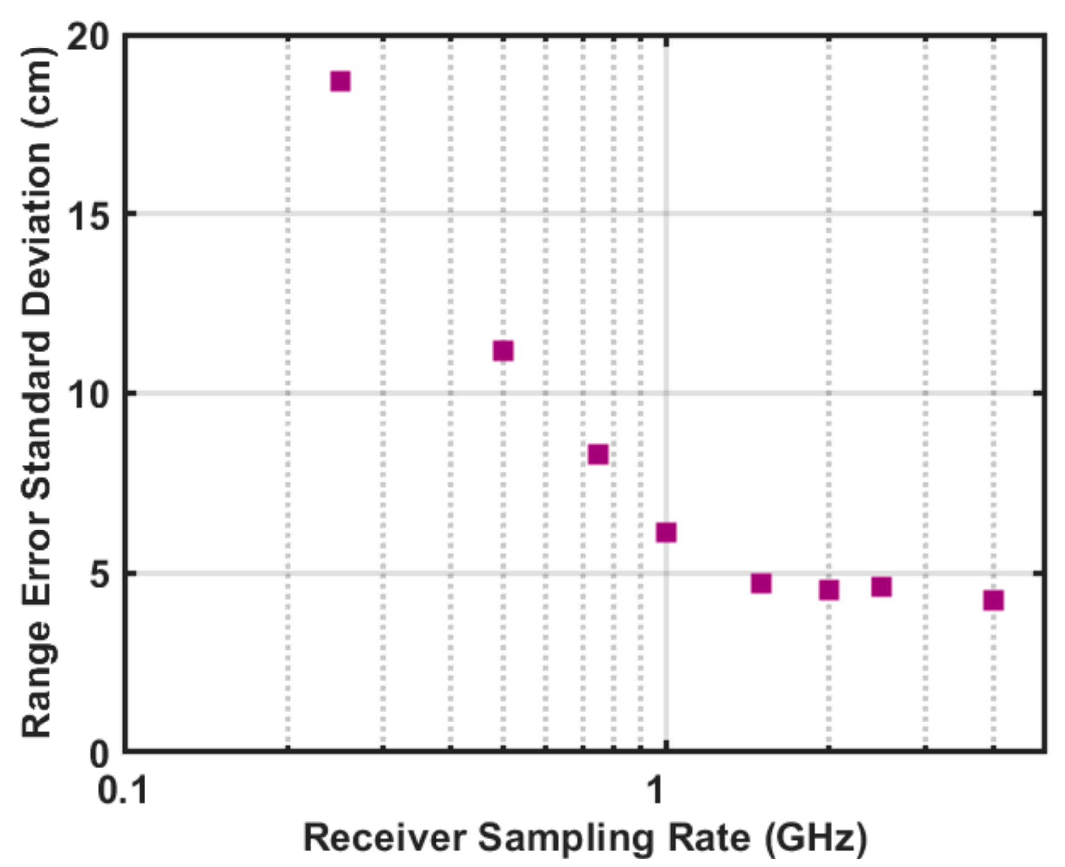
Figure 2.
Cross-correlation results comparing various methods of extending PN code and kernel to 2N. All codes were given a synthetic range of 10,000 prior to cross-correlation. (A) PN code correlation with 2N − 1 bits and other parameters from Table 1 (length: 65,024). (B) Correlation result after zero-padding of length 512 at the end of the code and kernel. (C) Correlation result after lengthening bit duration to 516 bins and zero-padding of length four at the end of the code and kernel. (D) Correlation result after resampling the code and kernel used in (A) to length 2N. The SNR is the peak value of the cross-correlation peak divided by the standard deviation of the cross-correlation at all other indices.
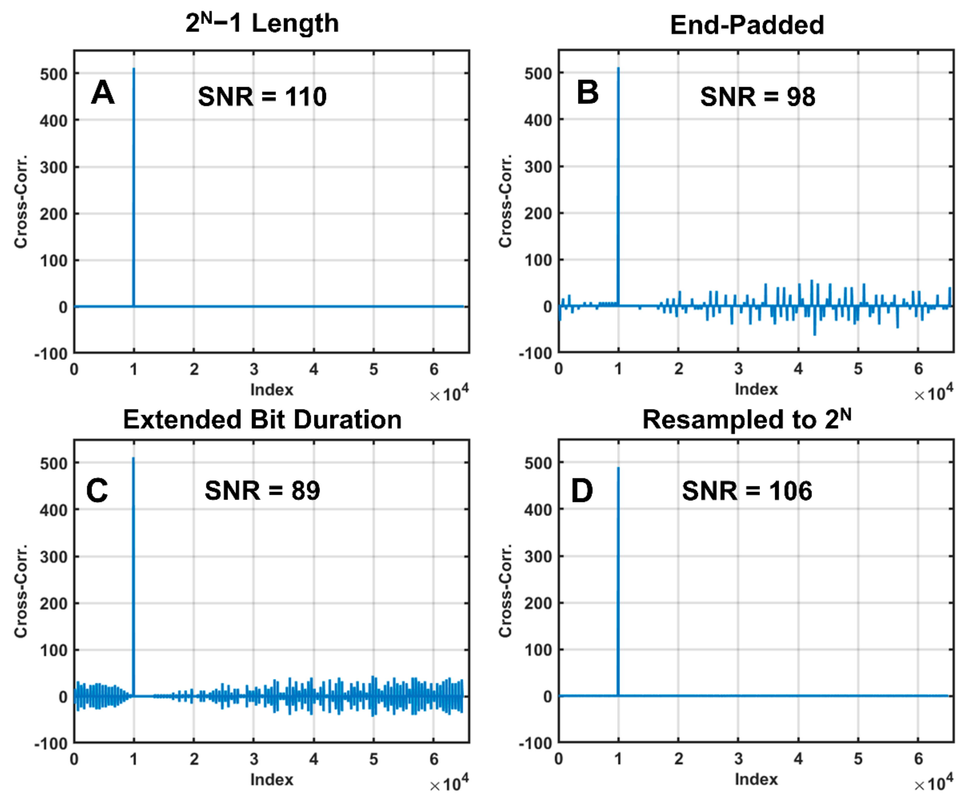
Figure 3.
Flowchart of the performance simulation for the PN code lidar. The steps in this chart are repeated for each distinct measurement in the simulation. The bold text indicates inputs for the simulation. The colored boxes correspond to simulation stages shown in Figure 4.
Figure 3.
Flowchart of the performance simulation for the PN code lidar. The steps in this chart are repeated for each distinct measurement in the simulation. The bold text indicates inputs for the simulation. The colored boxes correspond to simulation stages shown in Figure 4.

Figure 4.
Selected samples from the performance simulation. All horizontal axes correspond to time in microseconds. (A) Transmitted PN code as a function of time. (B) Detector analog signal for a single code length prior to digitization is shown in red. The shorter blue signal corresponds to the range-shifted code. (C) Subset of (B) showing the individual photon detection events. The black, dotted line shows the threshold setting. (D) Digitized signal after the comparator stage. (E) Histogram of 154 accumulated digitized codes corresponding to a 10-ms integration time. (F) Cross-correlation of the histogram in (E) with the kernel, showing the correlation peak at 3.4 µs.

Figure 5.
Track location for SALi 101955 orbital simulation on the OLA v20 PTM shape model with a 9 pixel per degree basemap from Bennet et al. (2021) [37]. The ground track location is shown in blue and is ~475 m in length. The track runs from 80.5793°S and 222.81°E to 80.99088°N and 207.642°E.
Figure 5.
Track location for SALi 101955 orbital simulation on the OLA v20 PTM shape model with a 9 pixel per degree basemap from Bennet et al. (2021) [37]. The ground track location is shown in blue and is ~475 m in length. The track runs from 80.5793°S and 222.81°E to 80.99088°N and 207.642°E.
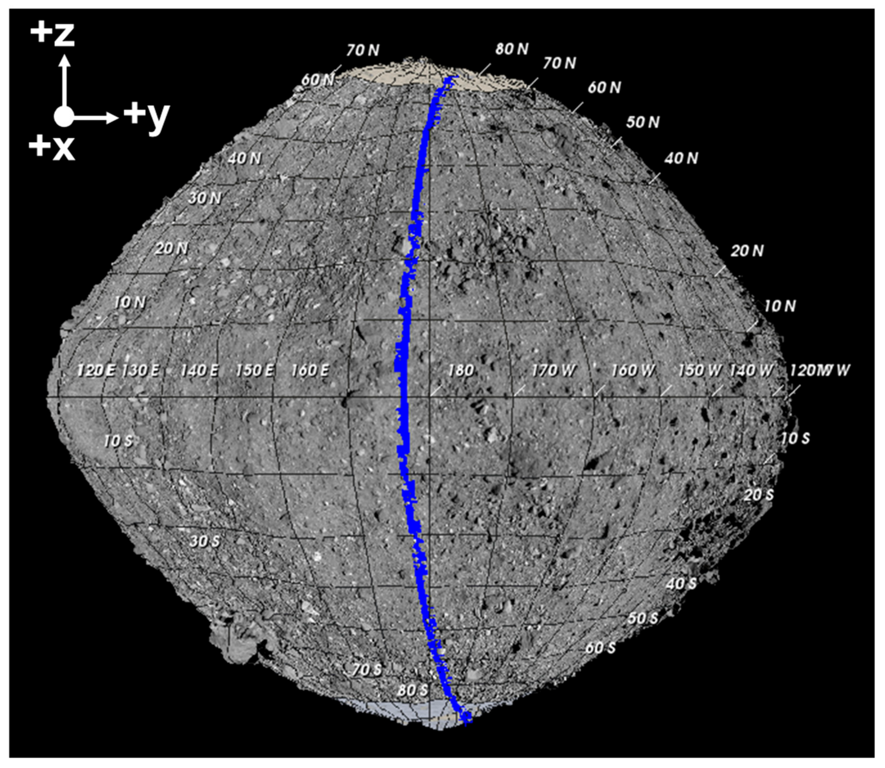
Figure 6.
One and two-photon simulated analog to digital conversion at 1.00787 GHz exhibiting the origin of the comparator bias and detected pulse width bias. (A) In the single photon case the comparator records six 1’s above the threshold for a single photon. Each 1 contributes to the peak amplitude of the cross-correlation, which leads to a positive bias if uncorrected. (B) Analog detector signal from two-photon detection, with the photons arriving 3 ns apart. The comparator records 10 1’s above the threshold, which is less than twice the single-photon value, leading to a negative bias.
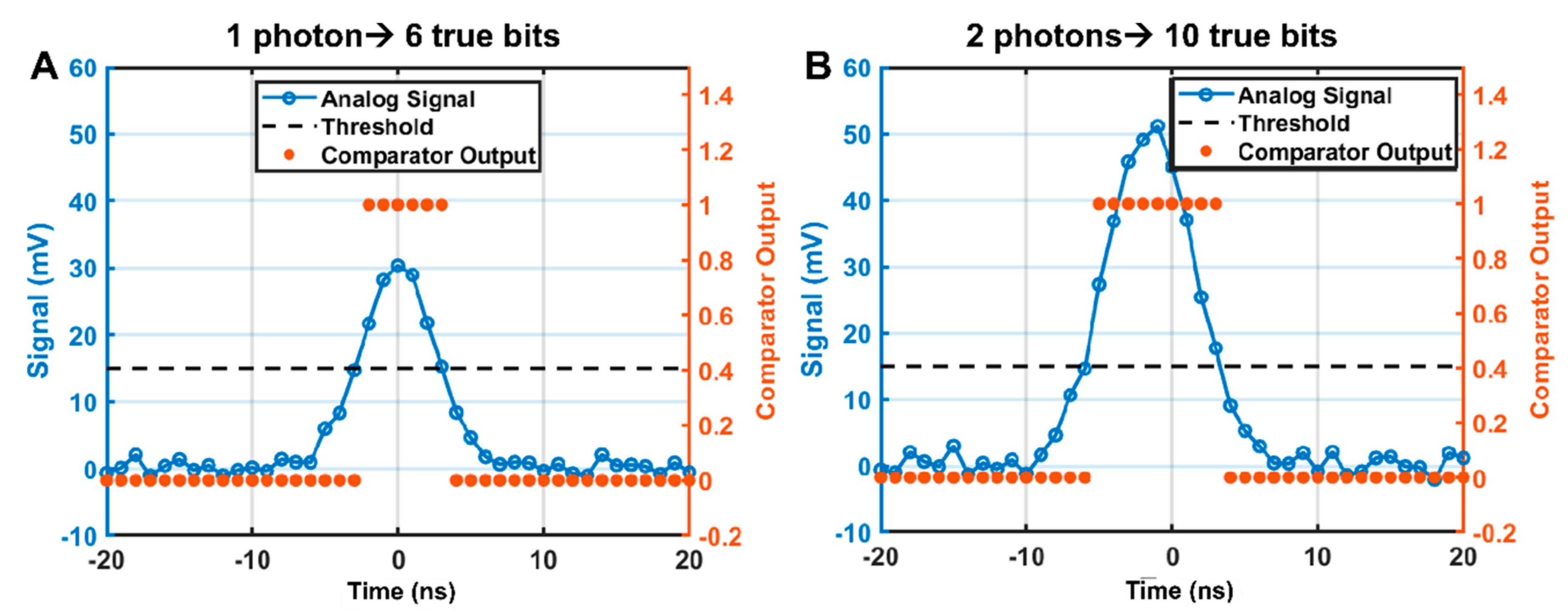
Figure 7.
Cross-correlation amplitude as a function of incident signal photon rate for 100 Hz measurement rate. For these simulations, the detector dark noise and solar background noise levels were set to zero.
Figure 7.
Cross-correlation amplitude as a function of incident signal photon rate for 100 Hz measurement rate. For these simulations, the detector dark noise and solar background noise levels were set to zero.

Figure 8.
Plot of SNR as a function of accumulated signal photons under various noise photon accumulation levels. The SNR is calculated as described in Section 2.1. An SNR < 6 corresponds to a probability of detection of <~80%. Each point corresponds to the average of five independent simulations. The lines denote best fit error functions for each accumulated noise level.

Figure 9.
Simulated SALi performance for the Reconnaissance mode conditions. (A) Full cross-correlation results. (B) Cross-correlation region near the cross-correlation peak. The range denotes the ambiguous range as determined from the PN code parameters. The SNR was determined as described in Section 2.1. The error is the absolute difference between the measured range via the threshold crossing method and the input synthetic range. The peak width is the difference between the rising and falling edge threshold crossings.

Figure 10.
Simulation results of the root mean squared ranging error and mean SNR as a function of target range for the SALi Mapping mode under (A) daytime and (B) nighttime conditions. Each point corresponds to five independent simulations. The exact range for each simulation was generated via a base range (ex. 100 km) and an additional randomly generated range between −1 and 1 m. The signal photon rates were calculated from the mean-removed cross-correlation peak, the laser pulse rate, and the integration time. The simulation assumed a flat surface (no range spreading). The vertical dotted line corresponds to the maximum range.

Figure 11.
Simulated SALi performance under nominal Mapping mode conditions following the conventions of Figure 9. (A) Full cross-correlation results. (B) Cross-correlation region near the cross-correlation peak. The simulation assumed a flat surface (no range spreading).
Figure 11.
Simulated SALi performance under nominal Mapping mode conditions following the conventions of Figure 9. (A) Full cross-correlation results. (B) Cross-correlation region near the cross-correlation peak. The simulation assumed a flat surface (no range spreading).
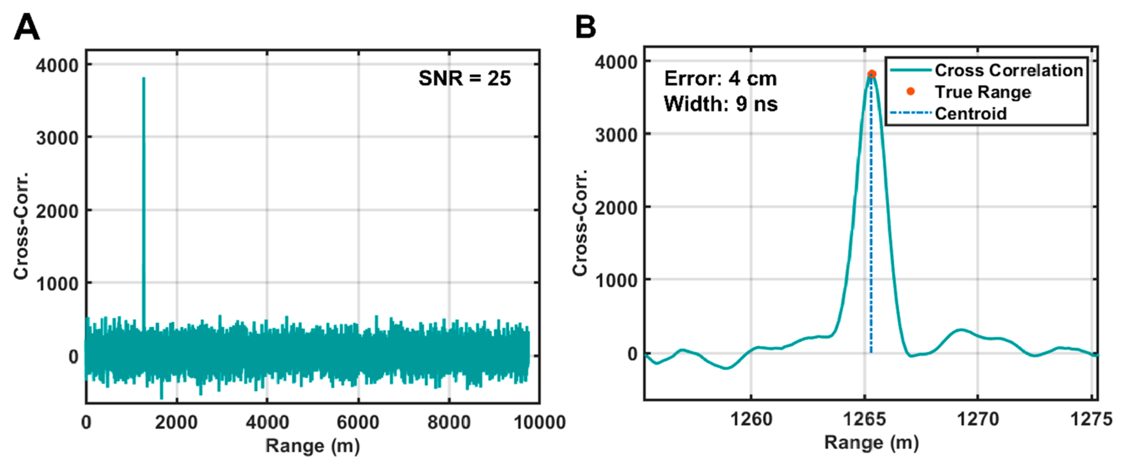
Figure 12.
Simulation results of SALi ranging performance as a function of target range for the SALi Mapping mode under (A) daytime and (B) nighttime conditions following the conventions of Figure 10. The simulation assumed a flat surface (no range spreading).
Figure 12.
Simulation results of SALi ranging performance as a function of target range for the SALi Mapping mode under (A) daytime and (B) nighttime conditions following the conventions of Figure 10. The simulation assumed a flat surface (no range spreading).

Figure 13.
PN ranging performance under varying levels of accumulated Doppler shift. The accumulated Doppler shift is normalized here as the ratio of the accumulated shift to the pulse length. (A) RMS ranging error and average SNR of five independent measurements at each accumulated Doppler shift following the conventions of Figure 10 and Figure 12. (B) Plots of a subset of cross-correlation peaks from the simulation in (A) showing the peak-spreading due to the Doppler the shift.

Figure 14.
Range from the spacecraft altitude to the Bennu surface and the retrieved range from the SALi performance simulation as a function of distance along track. Each blue marker represents one 10-ms measurement. The red line was generated from the interpolated ground track elevation. (inset) A portion of the track from 170 m to 300 m showing the range measurements tracking the elevation over sharp features in the surface terrain.

Figure 15.
Range residuals (measured minus actual) from the data shown in Figure 14. The ground-truth elevation value was taken as the mean of all ranges within the footprint.
Figure 15.
Range residuals (measured minus actual) from the data shown in Figure 14. The ground-truth elevation value was taken as the mean of all ranges within the footprint.
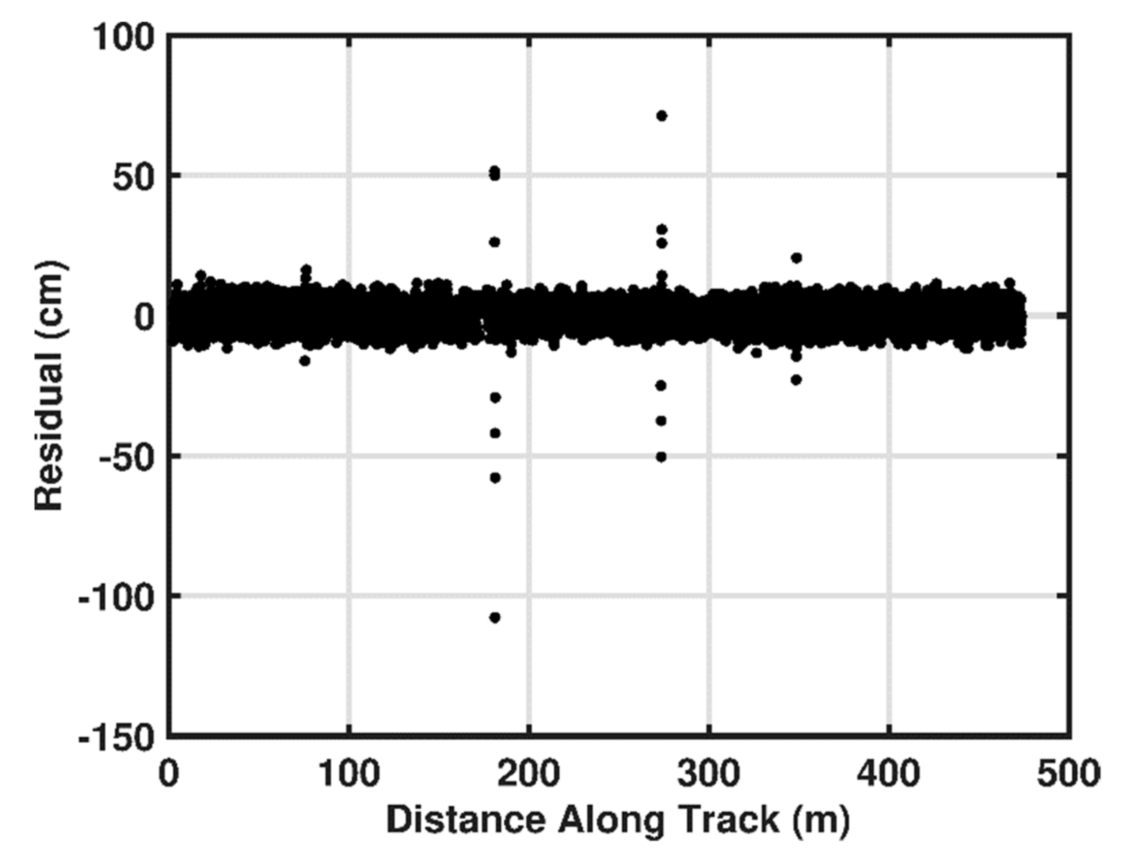
Figure 16.
A select region of the track exhibiting high range residuals. The blue markers and red line are the same as in Figure 14 and denote the SALi retrieved range and Bennu ground track from the shape model, respectively. The gold line denotes the size of the SALi footprint on the surface for the measurement at 183 m along the track. As the results are plotted as a function of range as measured by the lidar the Bennu surface normal points down in this plot.
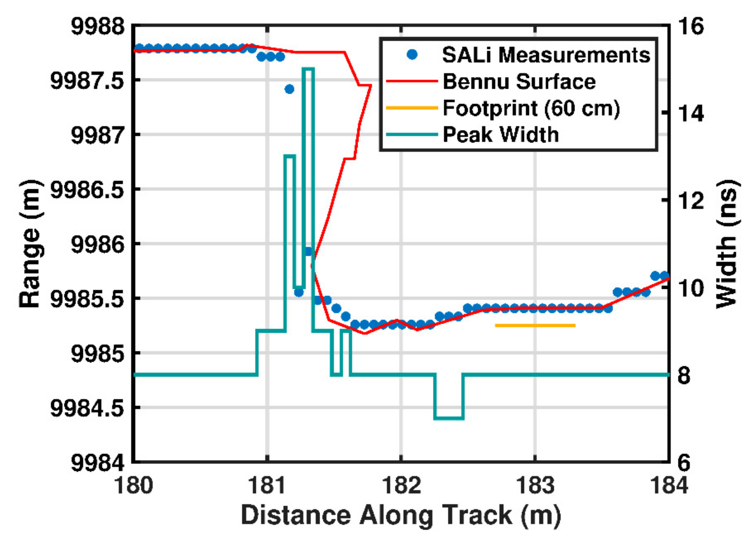
Figure 17.
Reflectance measurement results using the pre-computed calibration curves and laser power control. Each point denotes the average retrieved reflectance for five trials at each reflectance value. Error bars correspond to 1σ. The dashed black line has a slope of 1.
Figure 17.
Reflectance measurement results using the pre-computed calibration curves and laser power control. Each point denotes the average retrieved reflectance for five trials at each reflectance value. Error bars correspond to 1σ. The dashed black line has a slope of 1.

Figure 18.
Simplified block diagram of real-time processing breadboard. All modules were housed in an NI PXIe chassis and data passed between modules occurred over the backplane.
Figure 18.
Simplified block diagram of real-time processing breadboard. All modules were housed in an NI PXIe chassis and data passed between modules occurred over the backplane.

Figure 19.
FPGA cross-correlation results of PN code and kernel. (A) Continuous output from the IFFT core of the SALi processing pipeline normalized to the peak value. The cycles correspond to clock cycles of the pipelined IFFT code. (B) Cross-correlation peak from (A) translated into lag between code and kernel (i.e., ambiguous range). The circles represent the discrete IFFT values from which the centroid, width, and SNR were calculated.

Table 1.
SALi PN code parameters.
| Parameter | Value |
|---|---|
| Code Length | 127 bits |
| Bit Duration | 512 ns |
| Code Period | 65,024 ns |
| Pulse Duration | 8 ns |
| RZ Ratio | 64 |
| Laser Duty Cycle | 0.78125% |
| Bit rate (MHz) | 1.953125 MHz |
| Unambiguous Range | 9746.9 m |
| Signal Sampling Rate | 1.00787 GHz |
Table 2.
Instrument and target parameters used in the performance simulations for the SALi instrument.
Table 2.
Instrument and target parameters used in the performance simulations for the SALi instrument.
| Parameter | Value |
|---|---|
| Laser Wavelength | 1550 nm |
| Average Laser Output Power | 2 W |
| Solar Distance | 1 A.U. |
| Target Reflectance | 5% |
| Telescope Diameter | 6.4 cm |
| Bandpass Filter FWHM | 1 nm |
| Detector | 16-pixel HgCdTe APD |
| Pixel Layout | 2 × 8 |
| Pixel IFOV | 60 µrad |
| Detector Quantum Efficiency | 60% |
| Detector Dark Counts per Pixel | 250 kHz |
| Detector Response Time | 3 ns |
Publisher’s Note: MDPI stays neutral with regard to jurisdictional claims in published maps and institutional affiliations. |
© 2021 by the authors. Licensee MDPI, Basel, Switzerland. This article is an open access article distributed under the terms and conditions of the Creative Commons Attribution (CC BY) license (https://creativecommons.org/licenses/by/4.0/).
Share and Cite
MDPI and ACS Style
Cremons, D.R.; Sun, X.; Abshire, J.B.; Mazarico, E. Small PN-Code Lidar for Asteroid and Comet Missions—Receiver Processing and Performance Simulations. Remote Sens. 2021, 13, 2282. https://0-doi-org.brum.beds.ac.uk/10.3390/rs13122282
AMA Style
Cremons DR, Sun X, Abshire JB, Mazarico E. Small PN-Code Lidar for Asteroid and Comet Missions—Receiver Processing and Performance Simulations. Remote Sensing. 2021; 13(12):2282. https://0-doi-org.brum.beds.ac.uk/10.3390/rs13122282
Chicago/Turabian StyleCremons, Daniel R., Xiaoli Sun, James B. Abshire, and Erwan Mazarico. 2021. "Small PN-Code Lidar for Asteroid and Comet Missions—Receiver Processing and Performance Simulations" Remote Sensing 13, no. 12: 2282. https://0-doi-org.brum.beds.ac.uk/10.3390/rs13122282
Note that from the first issue of 2016, this journal uses article numbers instead of page numbers. See further details here.