
Pixel- vs. Object-Based Landsat 8 Data Classification in Google Earth Engine Using Random Forest: The Case Study of Maiella National Park


Abstract
:
1. Introduction
2. Materials and Methods
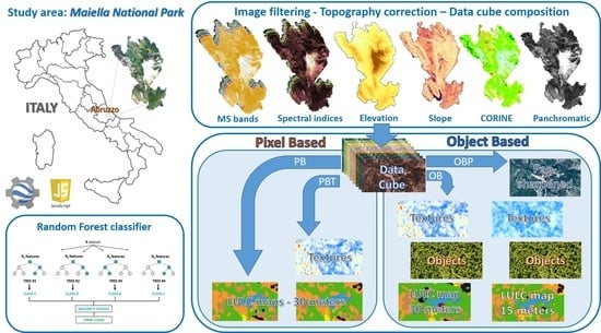
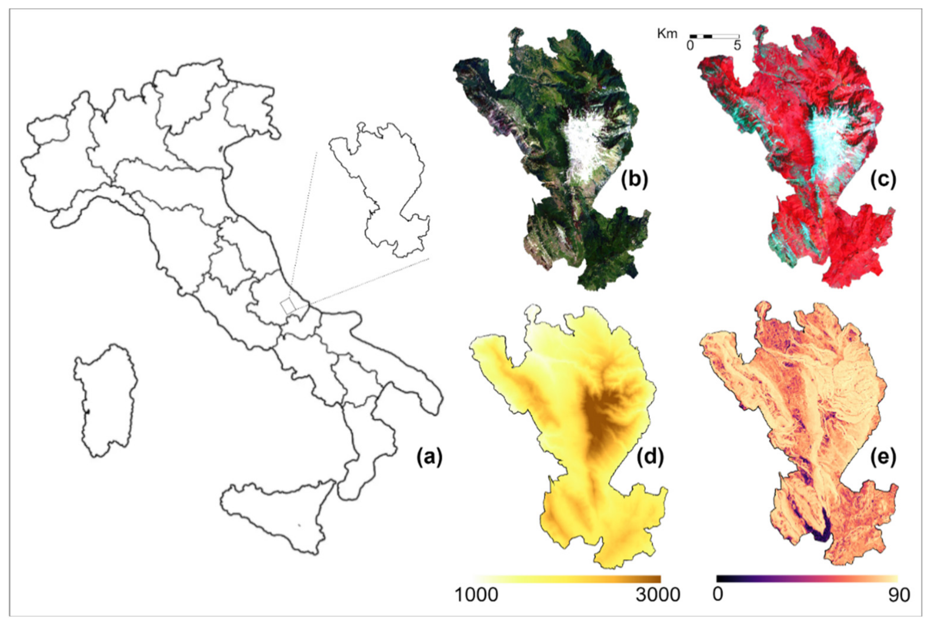
2.1. Study Area
2.2. Methodological Framework
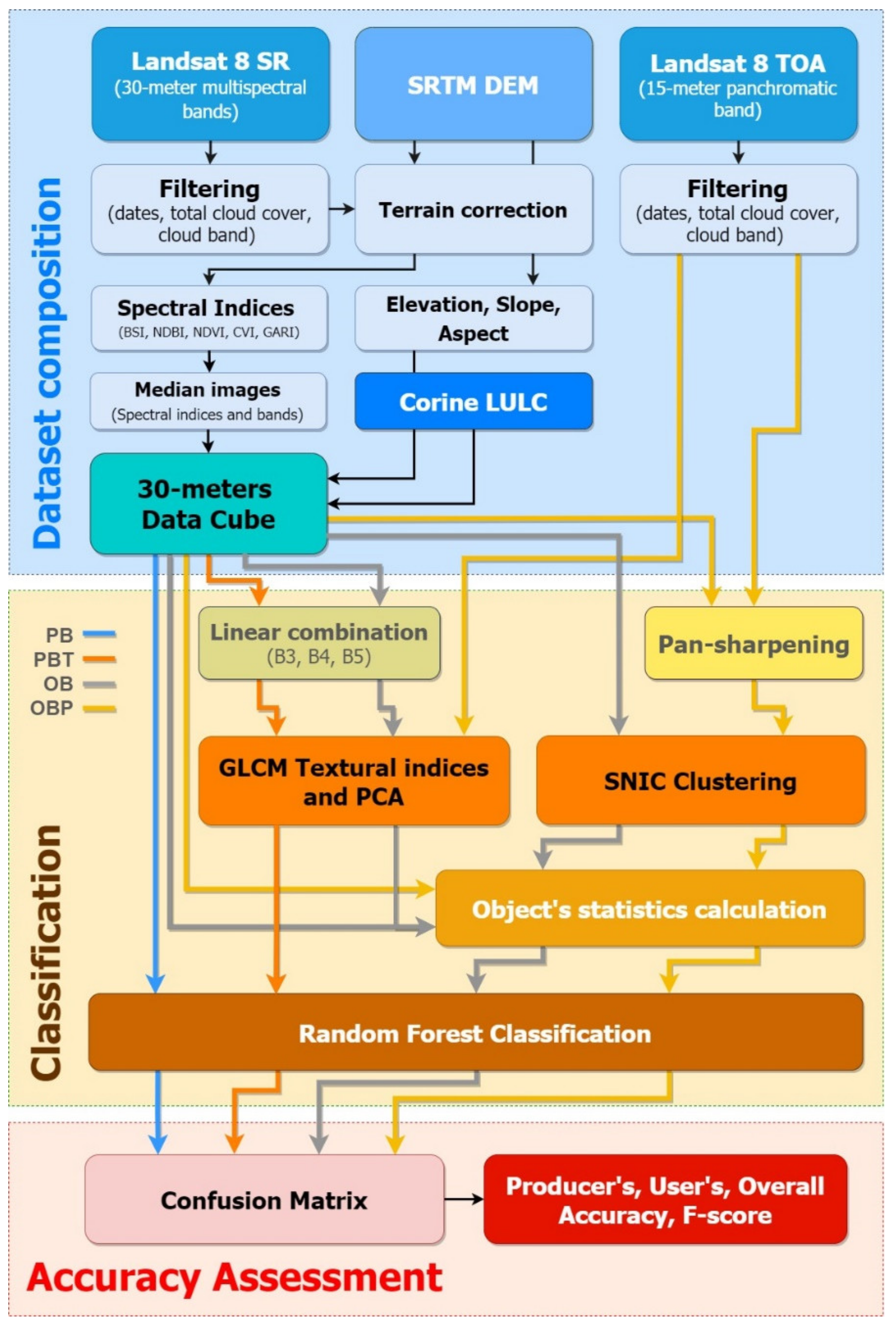
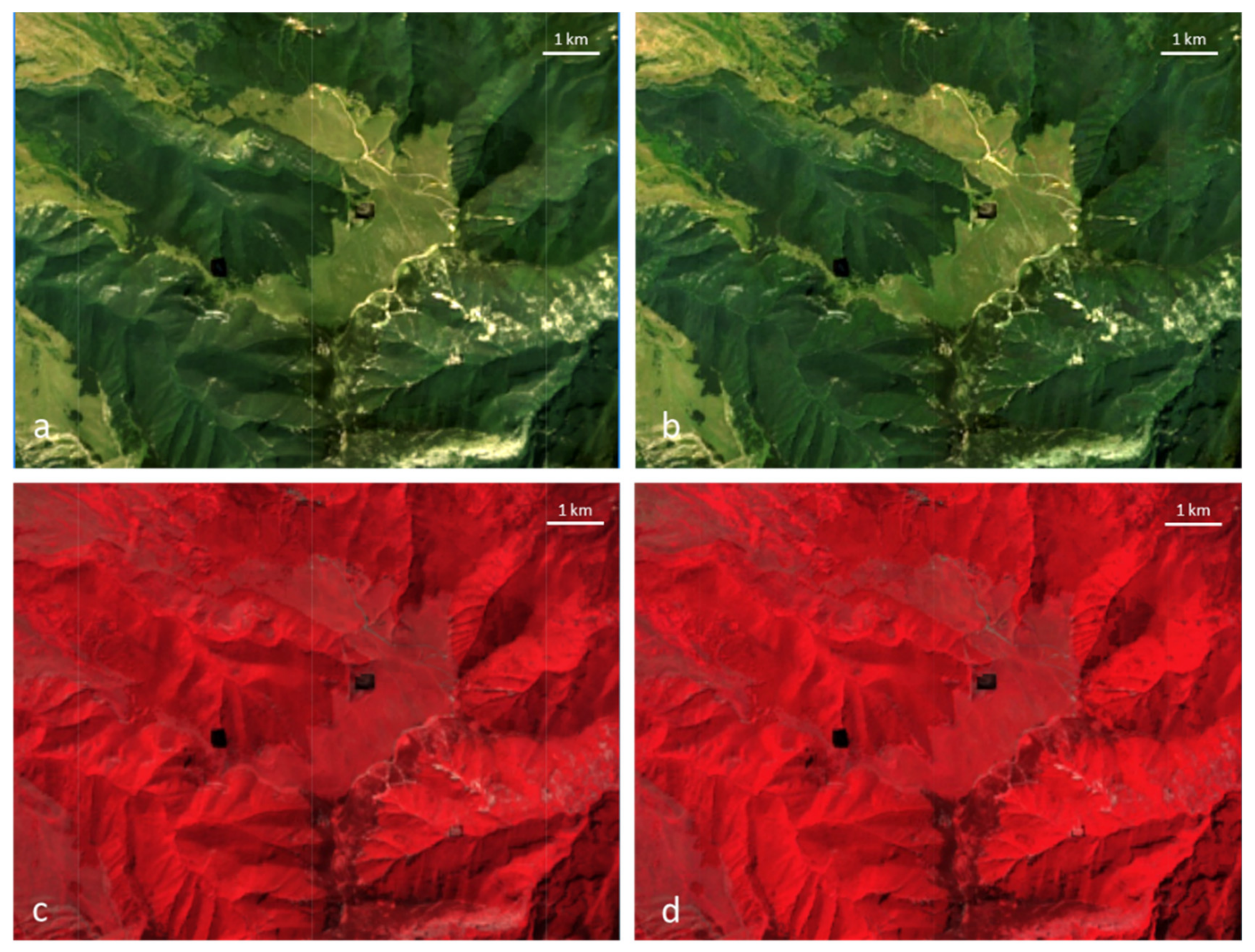
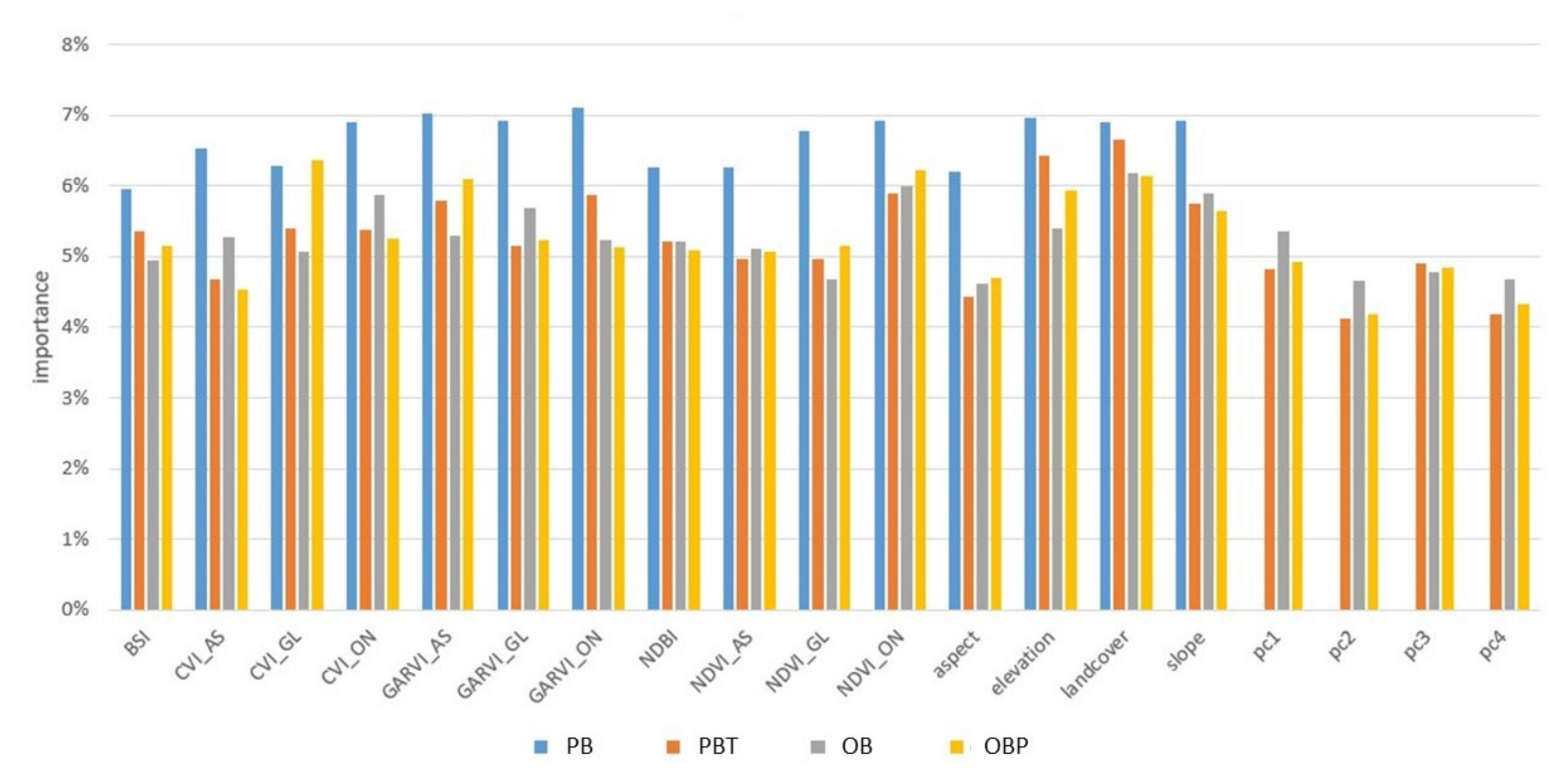
2.3. Data Composition
2.4. Classification
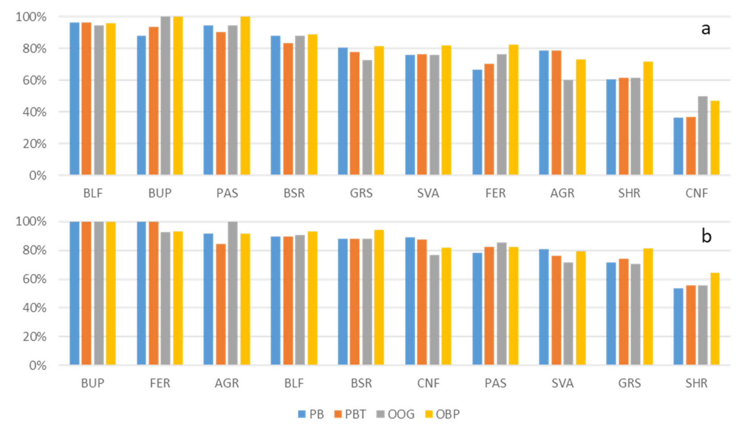
- Pixel-based (PB);
- Pixel-based including the image textural information (PBT);
- Object-Based, using BDC (OB);
- Object-Based, using the L8 15-m panchromatic band and the BDC (OBP).
2.5. Accuracy Assessment
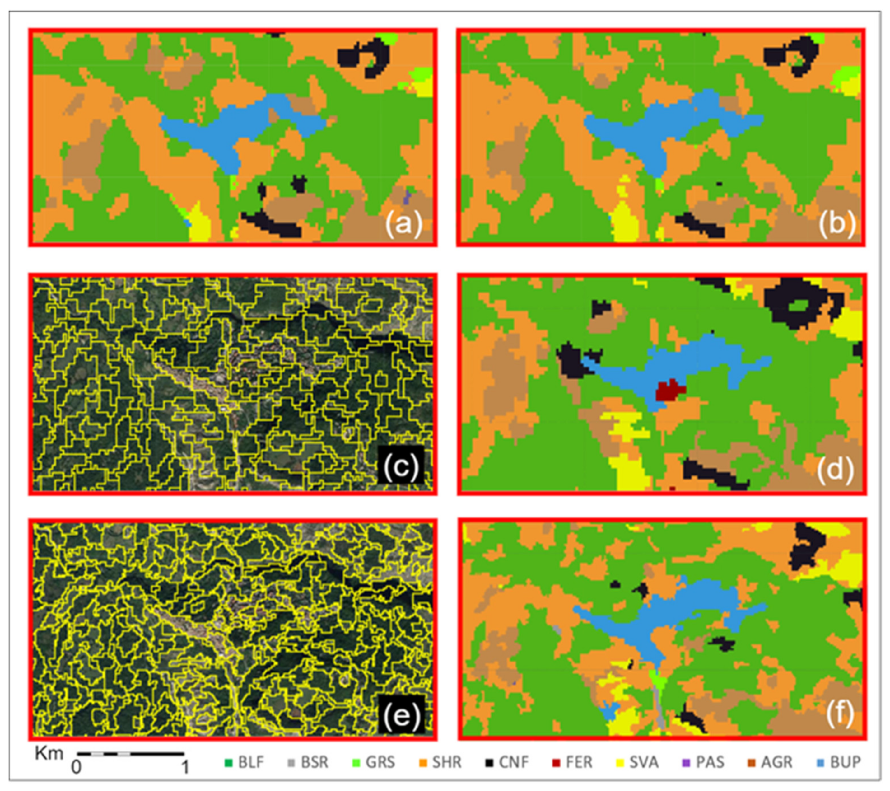
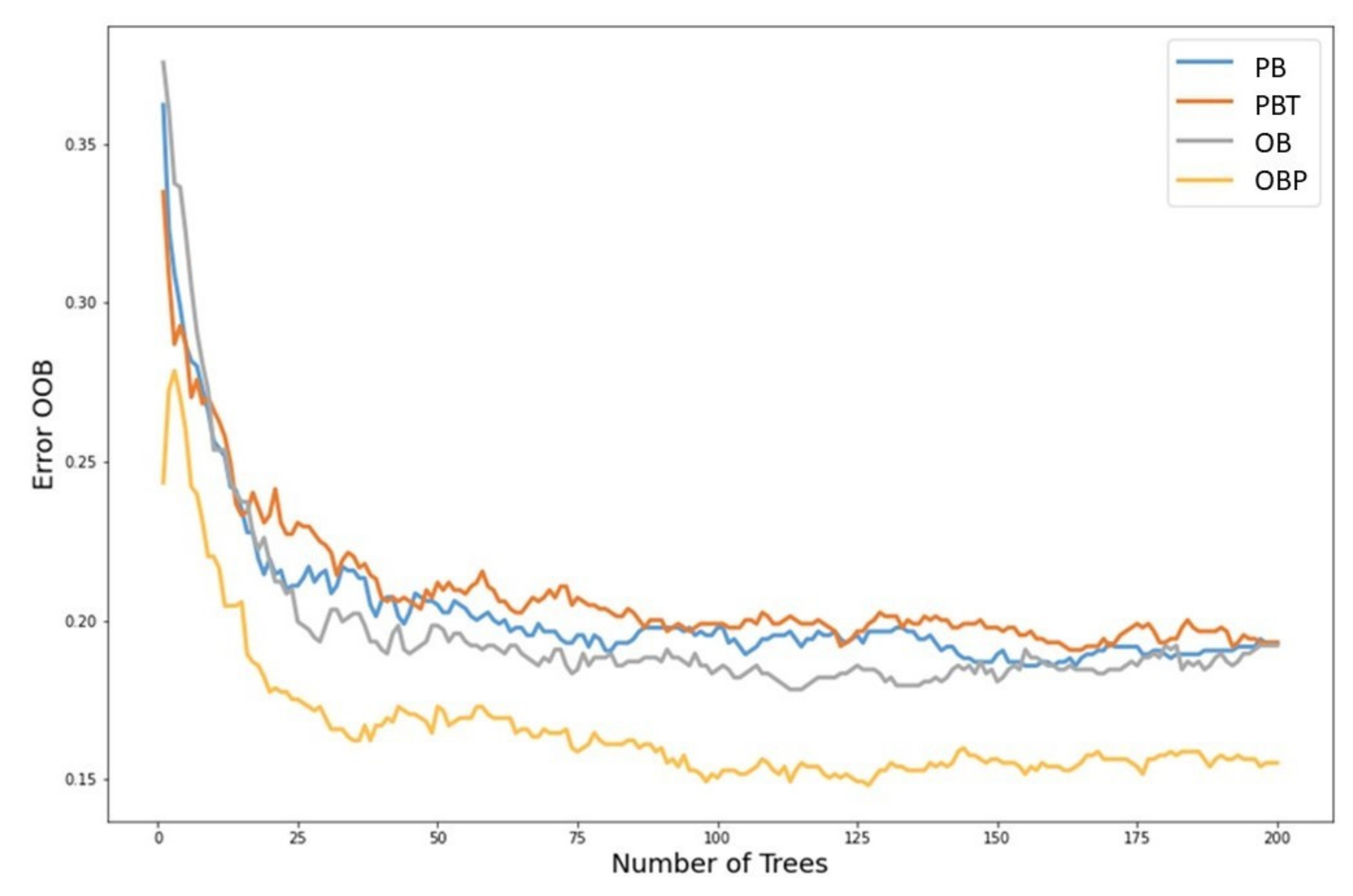
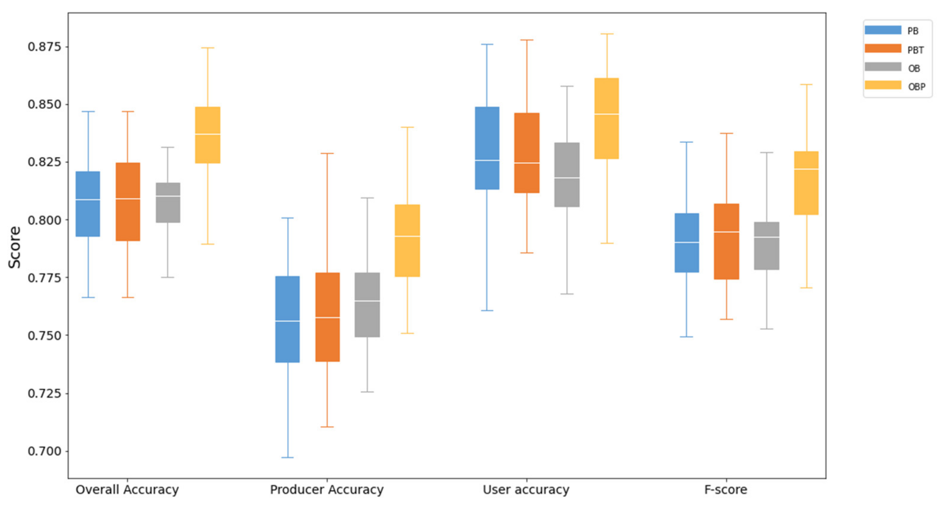
3. Results
4. Discussion
5. Conclusions
Author Contributions
Funding
Institutional Review Board Statement
Informed Consent Statement
Data Availability Statement
Conflicts of Interest
References
- Rawat, J.S.; Biswas, V.; Kumar, M. Changes in land use/cover using geospatial techniques: A case study of Ramnagar town area, district Nainital, Uttarakhand, India. Egypt. J. Remote Sens. Sp. Sci. 2013. [Google Scholar] [CrossRef] [Green Version]
- Antognelli, S.; Vizzari, M. Ecosystem and urban services for landscape liveability: A model for quantification of stakeholders’ perceived importance. Land Use Policy 2016, 50. [Google Scholar] [CrossRef]
- Antognelli, S.; Vizzari, M. Landscape liveability spatial assessment integrating ecosystem and urban services with their perceived importance by stakeholders. Ecol. Indic. 2017, 72, 703–725. [Google Scholar] [CrossRef]
- Padoch, C.; Brondizio, E.; Costa, S.; Pinedo-Vasquez, M.; Sears, R.R.; Siqueria, A. Urban forest and rural cities: Multi-sited households, consumption patterns, and forest resources in Amazonia. Ecol. Soc. 2008, 13. [Google Scholar] [CrossRef] [Green Version]
- Tassi, A.; Gil, A. A Low-cost Sentinel-2 Data and Rao’s Q Diversity Index-based Application for Detecting, Assessing and Monitoring Coastal Land-cover/Land-use Changes at High Spatial Resolution. J. Coast. Res. 2020. [Google Scholar] [CrossRef]
- Twisa, S.; Buchroithner, M.F. Land-use and land-cover (LULC) change detection in Wami river basin, Tanzania. Land 2019, 8, 136. [Google Scholar] [CrossRef] [Green Version]
- Fichera, C.R.; Modica, G.; Pollino, M. Land Cover classification and change-detection analysis using multi-temporal remote sensed imagery and landscape metrics. Eur. J. Remote Sens. 2012, 45, 1–18. [Google Scholar] [CrossRef]
- Modica, G.; Vizzari, M.; Pollino, M.; Fichera, C.R.R.; Zoccali, P.; Di Fazio, S. Spatio-temporal analysis of the urban–rural gradient structure: An application in a Mediterranean mountainous landscape (Serra San Bruno, Italy). Earth Syst. Dyn. 2012, 3, 263–279. [Google Scholar] [CrossRef] [Green Version]
- Vizzari, M.; Sigura, M. Landscape sequences along the urban–rural–natural gradient: A novel geospatial approach for identification and analysis. Landsc. Urban Plan. 2015, 140, 42–55. [Google Scholar] [CrossRef]
- Vizzari, M.; Hilal, M.; Sigura, M.; Antognelli, S.; Joly, D. Urban-rural-natural gradient analysis with CORINE data: An application to the metropolitan France. Landsc. Urban Plan. 2018. [Google Scholar] [CrossRef]
- Gorelick, N.; Hancher, M.; Dixon, M.; Ilyushchenko, S.; Thau, D.; Moore, R. Remote Sensing of Environment Google Earth Engine: Planetary-scale geospatial analysis for everyone. Remote Sens. Environ. 2017. [Google Scholar] [CrossRef]
- Griffiths, P.; van der Linden, S.; Kuemmerle, T.; Hostert, P. A Pixel-Based Landsat Compositing Algorithm for Large Area Land Cover Mapping. IEEE J. Sel. Top. Appl. Earth Obs. Remote Sens. 2013. [Google Scholar] [CrossRef]
- Irons, J.R.; Dwyer, J.L.; Barsi, J.A. The next Landsat satellite: The Landsat Data Continuity Mission. Remote Sens. Environ. 2012, 122, 11–21. [Google Scholar] [CrossRef] [Green Version]
- Available online: https://developers.google.com/earth-engine/datasets/catalog/LANDSAT_LC08_C01_T1_SR#description (accessed on 1 June 2021).
- Available online: https://developers.google.com/earth-engine/datasets/catalog/LANDSAT_LC08_C01_T1_TOA (accessed on 1 June 2021).
- Available online: http://gsp.humboldt.edu/OLM/Courses/GSP_216_Online/lesson4-1/pan-sharpen.html (accessed on 1 June 2021).
- Modica, G.; Solano, F.; Merlino, A.; Di Fazio, S.; Barreca, F.; Laudari, L.; Fichera, C.R. Using landsat 8 imagery in detecting cork oak (Quercus suber L.) Woodlands: A case study in Calabria (Italy). J. Agric. Eng. 2016, 47, 205–215. [Google Scholar] [CrossRef] [Green Version]
- Pfeifer, M.; Disney, M.; Quaife, T.; Marchant, R. Terrestrial ecosystems from space: A review of earth observation products for macroecology applications. Glob. Ecol. Biogeogr. 2011, 21, 603–624. [Google Scholar] [CrossRef] [Green Version]
- Blaschke, T. Object based image analysis for remote sensing. ISPRS J Photogramm Remote Sens. ISPRS J. Photogramm. Remote Sens. 2010, 65, 2–16. [Google Scholar] [CrossRef] [Green Version]
- Solano, F.; Di Fazio, S.; Modica, G. A methodology based on GEOBIA and WorldView-3 imagery to derive vegetation indices at tree crown detail in olive orchards. Int. J. Appl. Earth Obs. Geoinf. 2019, 83, 101912. [Google Scholar] [CrossRef]
- Ren, X.; Malik, J. Learning a classification model for segmentation. In Proceedings of the IEEE International Conference on Computer Vision, Nice, France, 13–16 October 2003. [Google Scholar]
- Flanders, D.; Hall-Beyer, M.; Pereverzoff, J. Preliminary evaluation of eCognition object-based software for cut block delineation and feature extraction. Can. J. Remote Sens. 2003. [Google Scholar] [CrossRef]
- Tassi, A.; Vizzari, M. Object-Oriented LULC Classification in Google Earth Engine Combining SNIC, GLCM, and Machine Learning Algorithms. Remote Sens. 2020, 12, 3776. [Google Scholar] [CrossRef]
- Labib, S.M.; Harris, A. The potentials of Sentinel-2 and LandSat-8 data in green infrastructure extraction, using object based image analysis (OBIA) method. Eur. J. Remote Sens. 2018. [Google Scholar] [CrossRef]
- Zhang, C.; Li, X.; Wu, M.; Qin, W.; Zhang, J. Object-oriented Classification of Land Cover Based on Landsat 8 OLI Image Data in the Kunyu Mountain. Sci. Geogr. Sin. 2018, 38, 1904–1913. [Google Scholar]
- Achanta, R.; Süsstrunk, S. Superpixels and polygons using simple non-iterative clustering. In Proceedings of the 30th IEEE Conference on Computer Vision and Pattern Recognition, CVPR 2017, Honolulu, HI, USA, 21–26 July 2017. [Google Scholar]
- Mahdianpari, M.; Salehi, B.; Mohammadimanesh, F.; Homayouni, S.; Gill, E. The first wetland inventory map of newfoundland at a spatial resolution of 10 m using sentinel-1 and sentinel-2 data on the Google Earth Engine cloud computing platform. Remote Sens. 2019, 11, 43. [Google Scholar] [CrossRef] [Green Version]
- Xiong, J.; Thenkabail, P.S.; Tilton, J.C.; Gumma, M.K.; Teluguntla, P.; Oliphant, A.; Congalton, R.G.; Yadav, K.; Gorelick, N. Nominal 30-m cropland extent map of continental Africa by integrating pixel-based and object-based algorithms using Sentinel-2 and Landsat-8 data on google earth engine. Remote Sens. 2017, 9, 1065. [Google Scholar] [CrossRef] [Green Version]
- Ghorbanian, A.; Kakooei, M.; Amani, M.; Mahdavi, S.; Mohammadzadeh, A.; Hasanlou, M. Improved land cover map of Iran using Sentinel imagery within Google Earth Engine and a novel automatic workflow for land cover classification using migrated training samples. ISPRS J. Photogramm. Remote Sens. 2020, 167, 276–288. [Google Scholar] [CrossRef]
- Mohanaiah, P.; Sathyanarayana, P.; Gurukumar, L. Image Texture Feature Extraction Using GLCM Approach. Int. J. Sci. Res. Publ. 2013, 3, 1–5. [Google Scholar]
- Godinho, S.; Guiomar, N.; Gil, A. Estimating tree canopy cover percentage in a mediterranean silvopastoral systems using Sentinel-2A imagery and the stochastic gradient boosting algorithm. Int. J. Remote Sens. 2018. [Google Scholar] [CrossRef]
- Mananze, S.; Pôças, I.; Cunha, M. Mapping and assessing the dynamics of shifting agricultural landscapes using google earth engine cloud computing, a case study in Mozambique. Remote Sens. 2020, 12, 1279. [Google Scholar] [CrossRef] [Green Version]
- Maleknezhad Yazdi, A.; Eisavi, V.; Shahsavari, A. İran Tahran şehri güney bölgesinde kent alanlarının sınıflandırılmasında SVM yöntemi ile hiperspektral görüntü ve tekstür bilgilerinin birlikte kullanılması. İstanbul Üniversitesi Orman Fakültesi Derg. 2016. [Google Scholar] [CrossRef]
- Nejad, A.M.; Ghassemian, H.; Mirzapour, F. GLCM Texture Features Efficiency Assessment of Pansharpened Hyperspectral Image Classification for Residential and Industrial Regions in Southern Tehran. J. Geomat. Sci. Technol. 2015, 5, 55–64. [Google Scholar]
- Mengge, T. Assessing the Value of Superpixel Approaches to Delineate Agricultural Parcels. Master’s Thesis, University of Twente, Enschede, Holland, 2019. [Google Scholar]
- Wu, C.F.; Deng, J.S.; Wang, K.; Ma, L.G.; Tahmassebi, A.R.S. Object-based classification approach for greenhouse mapping using Landsat-8 imagery. Int. J. Agric. Biol. Eng. 2016. [Google Scholar] [CrossRef]
- Nery, T.; Sadler, R.; Solis-Aulestia, M.; White, B.; Polyakov, M.; Chalak, M. Comparing supervised algorithms in Land Use and Land Cover classification of a Landsat time-series. In Proceedings of the International Geoscience and Remote Sensing Symposium (IGARSS), Beijing, China, 3 November 2016. [Google Scholar]
- Mather, P.; Tso, B. Classification Methods for Remotely Sensed Data, 2nd ed.; CRC Press, Engineering and Technology, Environment and Agriculture: Boca Raton, FL, USA, 2016; ISBN 9781420090741. [Google Scholar] [CrossRef]
- Breiman, L. Random forests. Mach. Learn. 2001. [Google Scholar] [CrossRef] [Green Version]
- Gislason, P.O.; Benediktsson, J.A.; Sveinsson, J.R. Random forests for land cover classification. In Pattern Recognition Letters; Elsevier Science: New York, NY, USA, 2006. [Google Scholar] [CrossRef]
- Mountrakis, G.; Im, J.; Ogole, C. Support vector machines in remote sensing: A review. ISPRS J. Photogramm. Remote Sens. 2011, 66, 247–259. [Google Scholar] [CrossRef]
- Amani, M.; Ghorbanian, A.; Ahmadi, S.A.; Kakooei, M.; Moghimi, A.; Mirmazloumi, S.M.; Moghaddam, S.H.A.; Mahdavi, S.; Ghahremanloo, M.; Parsian, S.; et al. Google Earth Engine Cloud Computing Platform for Remote Sensing Big Data Applications: A Comprehensive Review. IEEE J. Sel. Top. Appl. Earth Obs. Remote Sens. 2020, 13, 5326–5350. [Google Scholar] [CrossRef]
- Praticò, S.; Solano, F.; Di Fazio, S.; Modica, G. Machine Learning Classification of Mediterranean Forest Habitats in Google Earth Engine Based on Seasonal Sentinel-2 Time-Series and Input Image Composition Optimisation. Remote Sens. 2021, 13, 586. [Google Scholar] [CrossRef]
- Rodriguez-Galiano, V.F.; Ghimire, B.; Rogan, J.; Chica-Olmo, M.; Rigol-Sanchez, J.P. An assessment of the effectiveness of a random forest classifier for land-cover classification. ISPRS J. Photogramm. Remote Sens. 2012. [Google Scholar] [CrossRef]
- Conti, F.; Ciaschetti, G.; Di Martino, L.; Bartolucci, F. An annotated checklist of the vascular flora of Majella national park (Central Italy). Phytotaxa 2019, 412, 1–90. [Google Scholar] [CrossRef]
- Di Cecco, V.; Di Santo, M.; Di Musciano, M.; Manzi, A.; Di Cecco, M.; Ciaschetti, G.; Marcantonio, G.; Di Martino, L. The Majella national park: A case study for the conservation of plant biodiversity in the Italian apennines. Ital. Bot. 2020, 10, 1–24. [Google Scholar] [CrossRef]
- Liberatoscioli, E.; Boscaino, G.; Agostini, S.; Garzarella, A.; Scandone, E. The Majella National Park: An aspiring UNESCO geopark. Geosciences 2018, 8, 256. [Google Scholar] [CrossRef] [Green Version]
- Available online: http://www.parks.it/parco.nazionale.majella/Epar.php (accessed on 1 June 2021).
- Xie, S.; Liu, L.; Zhang, X.; Yang, J.; Chen, X.; Gao, Y. Automatic land-cover mapping using landsat time-series data based on google earth engine. Remote Sens. 2019, 11, 3023. [Google Scholar] [CrossRef] [Green Version]
- Nyland, K.E.; Gunn, G.E.; Shiklomanov, N.I.; Engstrom, R.N.; Streletskiy, D.A. Land cover change in the lower Yenisei River using dense stacking of landsat imagery in Google Earth Engine. Remote Sens. 2018, 10, 1226. [Google Scholar] [CrossRef] [Green Version]
- Richter, R.; Kellenberger, T.; Kaufmann, H. Comparison of topographic correction methods. Remote Sens. 2009, 10, 184. [Google Scholar] [CrossRef] [Green Version]
- Soenen, S.A.; Peddle, D.R.; Coburn, C.A. SCS+C: A modified sun-canopy-sensor topographic correction in forested terrain. IEEE Trans. Geosci. Remote Sens. 2005. [Google Scholar] [CrossRef]
- Vanonckelen, S.; Lhermitte, S.; Balthazar, V.; Van Rompaey, A. Performance of atmospheric and topographic correction methods on Landsat imagery in mountain areas. Int. J. Remote Sens. 2014. [Google Scholar] [CrossRef] [Green Version]
- Belcore, E.; Piras, M.; Wozniak, E. Specific alpine environment land cover classification methodology: Google earth engine processing for sentinel-2 data. In Proceedings of the International Archives of the Photogrammetry, Remote Sensing and Spatial Information Sciences-ISPRS Archives, Nice, France, 31 August–2 September 2020. [Google Scholar]
- Shepherd, J.D.; Dymond, J.R. Correcting satellite imagery for the variance of reflectance and illumination with topography. Int. J. Remote Sens. 2003. [Google Scholar] [CrossRef]
- Burns, P.; Macander, M. Topographic Correction in GEE–Open Geo Blog. Available online: https://mygeoblog.com/2018/10/17/terrain-correction-in-gee/ (accessed on 25 February 2021).
- Singh, R.P.; Singh, N.; Singh, S.; Mukherjee, S. Normalized Difference Vegetation Index (NDVI) Based Classification to Assess the Change in Land Use/Land Cover (LULC) in Lower Assam, India. Int. J. Adv. Remote Sens. GIS 2016. [Google Scholar] [CrossRef]
- Capolupo, A.; Monterisi, C.; Tarantino, E. Landsat Images Classification Algorithm (LICA) to Automatically Extract Land Cover Information in Google Earth Engine Environment. Remote Sens. 2020, 12, 1201. [Google Scholar] [CrossRef] [Green Version]
- Polykretis, C.; Grillakis, M.G.; Alexakis, D.D. Exploring the impact of various spectral indices on land cover change detection using change vector analysis: A case study of Crete Island, Greece. Remote Sens. 2020, 2, 319. [Google Scholar] [CrossRef] [Green Version]
- Diek, S.; Fornallaz, F.; Schaepman, M.E.; de Jong, R. Barest Pixel Composite for agricultural areas using landsat time series. Remote Sens. 2017, 9, 1245. [Google Scholar] [CrossRef] [Green Version]
- Chen, W.; Liu, L.; Zhang, C.; Wang, J.; Wang, J.; Pan, Y. Monitoring the seasonal bare soil areas in Beijing using multi-temporal TM images. In Proceedings of the International Geoscience and Remote Sensing Symposium (IGARSS), Anchorage, AK, USA, 20–24 September 2004. [Google Scholar]
- Zha, Y.; Gao, J.; Ni, S. Use of normalized difference built-up index in automatically mapping urban areas from TM imagery. Int. J. Remote Sens. 2003. [Google Scholar] [CrossRef]
- Bhatti, S.S.; Tripathi, N.K. Built-up area extraction using Landsat 8 OLI imagery. GIScience Remote Sens. 2014, 51, 445–467. [Google Scholar] [CrossRef] [Green Version]
- Ghosh, D.K.; Mandal, A.C.H.; Majumder, R.; Patra, P.; Bhunia, G.S. Analysis for mapping of built-up area using remotely sensed indices-A case study of rajarhat block in Barasat sadar sub-division in west Bengal (India). J. Landsc. Ecol. Repub. 2018. [Google Scholar] [CrossRef] [Green Version]
- Rikimaru, A.; Roy, P.S.; Miyatake, S. Tropical forest cover density mapping. Trop. Ecol. 2002, 43, 39–47. [Google Scholar]
- Rouse, J.W., Jr.; Haas, R.H.; Schell, J.A.; Deering, D.W. Monitoring vegetation systems in the great plains with erts. In Proceedings of the NASA SP-351, 3rd ERTS-1 Symposium, Greenbelt, Maryland, 29 July 1974; pp. 309–317. [Google Scholar]
- Gitelson, A.A.; Kaufman, Y.J.; Merzlyak, M.N. Use of a green channel in remote sensing of global vegetation from EOS- MODIS. Remote Sens. Environ. 1996, 58, 289–298. [Google Scholar] [CrossRef]
- Vincini, M.; Frazzi, E.; D’Alessio, P. A broad-band leaf chlorophyll vegetation index at the canopy scale. Precis. Agric. 2008, 9, 303–319. [Google Scholar] [CrossRef]
- Kobayashi, N.; Tani, H.; Wang, X.; Sonobe, R. Crop classification using spectral indices derived from Sentinel-2A imagery. J. Inf. Telecommun. 2020. [Google Scholar] [CrossRef]
- Available online: https://land.copernicus.eu/pan-european/corine-land-cover (accessed on 1 June 2021).
- Grohmann, C.H. Effects of spatial resolution on slope and aspect derivation for regional-scale analysis. Comput. Geosci. 2015. [Google Scholar] [CrossRef] [Green Version]
- Meher, P.K.; Sahu, T.K.; Rao, A.R. Prediction of donor splice sites using random forest with a new sequence encoding approach. BioData Min. 2016. [Google Scholar] [CrossRef]
- Oshiro, T.M.; Perez, P.S.; Baranauskas, J.A. How many trees in a random forest? In Proceedings of the Lecture Notes in Computer Science (including subseries Lecture Notes in Artificial Intelligence and Lecture Notes in Bioinformatics), Berlin, Germany, 13–20 July 2012. [Google Scholar]
- Ozigis, M.S.; Kaduk, J.D.; Jarvis, C.H.; da Conceição Bispo, P.; Balzter, H. Detection of oil pollution impacts on vegetation using multifrequency SAR, multispectral images with fuzzy forest and random forest methods. Environ. Pollut. 2020. [Google Scholar] [CrossRef]
- Probst, P.; Boulesteix, A.L. To tune or not to tune the number of trees in random forest. J. Mach. Learn. Res. 2018, 18, 1–18. [Google Scholar]
- Ge, J.; Liu, H. Investigation of image classification using hog, glcm features, and svm classifier. In Proceedings of the Lecture Notes in Electrical Engineering, Singapore, 15 October 2020; Springer Science and Business Media Deutschland GmbH: Berlin/Heidelberg, Germany, 2020; Volume 645, pp. 411–417. [Google Scholar]
- Available online: https://developers.google.com/earth-engine/guides/image_transforms (accessed on 1 June 2021).
- Carta Della Natura—Italiano. Available online: https://www.isprambiente.gov.it/it/servizi/sistema-carta-della-natura (accessed on 25 March 2021).
- Mueller, J.P.; Massaron, L. Training, Validating, and Testing in Machine Learning. Available online: https://www.dummies.com/programming/big-data/data-science/training-validating-testing-machine-learning/ (accessed on 7 June 2021).
- Adelabu, S.; Mutanga, O.; Adam, E. Testing the reliability and stability of the internal accuracy assessment of random forest for classifying tree defoliation levels using different validation methods. Geocarto Int. 2015, 30, 810–821. [Google Scholar] [CrossRef]
- Chen, W.; Xie, X.; Wang, J.; Pradhan, B.; Hong, H.; Bui, D.T.; Duan, Z.; Ma, J. A comparative study of logistic model tree, random forest, and classification and regression tree models for spatial prediction of landslide susceptibility. Catena 2017, 151, 147–160. [Google Scholar] [CrossRef] [Green Version]
- Congalton, R.G. A review of assessing the accuracy of classifications of remotely sensed data. Remote Sens. Environ. 1991. [Google Scholar] [CrossRef]
- Liu, C.; Frazier, P.; Kumar, L. Comparative assessment of the measures of thematic classification accuracy. Remote Sens. Environ. 2007. [Google Scholar] [CrossRef]
- Al-Saady, Y.; Merkel, B.; Al-Tawash, B.; Al-Suhail, Q. Land use and land cover (LULC) mapping and change detection in the Little Zab River Basin (LZRB), Kurdistan Region, NE Iraq and NW Iran. FOG Freib. Online Geosci. 2015, 43, 1–32. [Google Scholar]
- Sokolova, M.; Japkowicz, N.; Szpakowicz, S. Beyond accuracy, F-score and ROC: A family of discriminant measures for performance evaluation. In Proceedings of the AAAI Workshop—Technical Report; Springer: Berlin, Heidelberg, December 2006. [Google Scholar]
- Taubenböck, H.; Esch, T.; Felbier, A.; Roth, A.; Dech, S. Pattern-based accuracy assessment of an urban footprint classification using TerraSAR-X data. IEEE Geosci. Remote Sens. Lett. 2011. [Google Scholar] [CrossRef]
- Stehman, S.V. Statistical rigor and practical utility in thematic map accuracy assessment. Photogramm. Eng. Remote Sens. 2001, 67, 727–734. [Google Scholar]
- Weaver, J.; Moore, B.; Reith, A.; McKee, J.; Lunga, D. A comparison of machine learning techniques to extract human settlements from high resolution imagery. In Proceedings of the International Geoscience and Remote Sensing Symposium (IGARSS), Valencia, Spain, 22–27 July 2018. [Google Scholar]
- Hurskainen, P.; Adhikari, H.; Siljander, M.; Pellikka, P.K.E.; Hemp, A. Auxiliary datasets improve accuracy of object-based land use/land cover classification in heterogeneous savanna landscapes. Remote Sens. Environ. 2019. [Google Scholar] [CrossRef]


| LULC Class | Code | Description |
|---|---|---|
| Broadleaf forests | BLF | Forest vegetation, dominated by different deciduous tree species, above all: beech, white oak, Turkey oak, and others. |
| Bare soil or rocks | BSR | Persistently non-vegetated areas characterized by bare soil or rocks. |
| Grasslands | GRS | Grassland vegetation dominated by grasses, forbs, and small shrubs in variable proportion, from dense and continuous to sparse and discontinuous, including both semi-natural secondary grasslands, up to ca. 1800 m. a.s.l., and primary grasslands at higher altitudes (above the tree limit). |
| Shrubs | SHR | Shrubs and scrublands mostly resulting from the abandonment of pastures and agricultural areas, from place to place dominated by brooms, juniperus, blackthorn, hawthorn, etc.; at higher altitudes, this class includes the natural potential vegetation of the subalpine belt, mainly dominated by dwarf juniper. |
| Coniferous | CNF | Coniferous stands, including both natural ones (i.e., Mugo Pine-dominated vegetation) and artificial plantations. |
| Ferns | FER | Pioneer dynamic stages, first steps of the successional processes occurring in abandoned pastures and agricultural areas, mostly represented by eagle fern-dominated vegetation [Pteridium aquilinum (L.) Kuhn subsp. aquilinum]. |
| Sparsely vegetated areas | SVA | Areas characterized by highly sparse and discontinuous vegetation cover, with a remarkable presence of stones and outcropping rocky substrate. |
| Pastures | PAS | Rich pastures and hay meadows with high biomass and dense cover values. |
| Agriculture | AGR | Agricultural areas. |
| Built-up | BUP | Built-up areas. |
Publisher’s Note: MDPI stays neutral with regard to jurisdictional claims in published maps and institutional affiliations. |
© 2021 by the authors. Licensee MDPI, Basel, Switzerland. This article is an open access article distributed under the terms and conditions of the Creative Commons Attribution (CC BY) license (https://creativecommons.org/licenses/by/4.0/).
Share and Cite
Tassi, A.; Gigante, D.; Modica, G.; Di Martino, L.; Vizzari, M. Pixel- vs. Object-Based Landsat 8 Data Classification in Google Earth Engine Using Random Forest: The Case Study of Maiella National Park. Remote Sens. 2021, 13, 2299. https://0-doi-org.brum.beds.ac.uk/10.3390/rs13122299
Tassi A, Gigante D, Modica G, Di Martino L, Vizzari M. Pixel- vs. Object-Based Landsat 8 Data Classification in Google Earth Engine Using Random Forest: The Case Study of Maiella National Park. Remote Sensing. 2021; 13(12):2299. https://0-doi-org.brum.beds.ac.uk/10.3390/rs13122299
Chicago/Turabian StyleTassi, Andrea, Daniela Gigante, Giuseppe Modica, Luciano Di Martino, and Marco Vizzari. 2021. "Pixel- vs. Object-Based Landsat 8 Data Classification in Google Earth Engine Using Random Forest: The Case Study of Maiella National Park" Remote Sensing 13, no. 12: 2299. https://0-doi-org.brum.beds.ac.uk/10.3390/rs13122299