
A Scalable, Supervised Classification of Seabed Sediment Waves Using an Object-Based Image Analysis Approach


1
Environmental Research Institute, School of Biological, Earth and Environmental Sciences, University College Cork, Distillery Fields, North Mall, T23 N73K Cork, Ireland
2
Green Rebel Group, Crosshaven Boatyard, Crosshaven, Co., P43 EV21 Cork, Ireland
3
Irish Centre for Applied Geosciences (ICRAG), Marine & Renewable Energy Institute (MaREI), University College Cork, T12 K8AF Cork, Ireland
*
Author to whom correspondence should be addressed.
Remote Sens. 2021, 13(12), 2317; https://0-doi-org.brum.beds.ac.uk/10.3390/rs13122317
Submission received: 11 May 2021
/
Revised: 4 June 2021
/
Accepted: 10 June 2021
/
Published: 13 June 2021
(This article belongs to the Section Remote Sensing Image Processing)
Abstract
:National mapping programs (e.g., INFOMAR and MAREANO) and global efforts (Seabed 2030) acquire large volumes of multibeam echosounder data to map large areas of the seafloor. Developing an objective, automated and repeatable approach to extract meaningful information from such vast quantities of data is now essential. Many automated or semi-automated approaches have been defined to achieve this goal. However, such efforts have resulted in classification schemes that are isolated or bespoke, and therefore it is necessary to form a standardised classification method. Sediment wave fields are the ideal platform for this as they maintain consistent morphologies across various spatial scales and influence the distribution of biological assemblages. Here, we apply an object-based image analysis (OBIA) workflow to multibeam bathymetry to compare the accuracy of four classifiers (two multilayer perceptrons, support vector machine, and voting ensemble) in identifying seabed sediment waves across three separate study sites. The classifiers are trained on high-spatial-resolution (0.5 m) multibeam bathymetric data from Cork Harbour, Ireland and are then applied to lower-spatial-resolution EMODnet data (25 m) from the Hemptons Turbot Bank SAC and offshore of County Wexford, Ireland. A stratified 10-fold cross-validation was enacted to assess overfitting to the sample data. Samples were taken from the lower-resolution sites and examined separately to determine the efficacy of classification. Results showed that the voting ensemble classifier achieved the most consistent accuracy scores across the high-resolution and low-resolution sites. This is the first object-based image analysis classification of bathymetric data able to cope with significant disparity in spatial resolution. Applications for this approach include benthic current speed assessments, a geomorphological classification framework for benthic biota, and a baseline for monitoring of marine protected areas.
1. Introduction
Vast amounts of high-resolution multibeam echosounder (MBES) data have been acquired and are further proposed in support of national (e.g., Ireland’s INFOMAR [1] and Norway’s MAREANO [2] projects) and global mapping efforts (e.g., the Nippon Foundation-GEBCO Project Seabed 2030 [3]). Thus, the need for a standardised classification system to extract meaningful seabed habitat relevant geomorphological information from these vast datasets is critical for marine spatial management [4]. Seabed habitats are not defined by the traditional frameworks evident in terrestrial habitats, and as such are characterised in terms of seabed geomorphology and sediment composition [5]. As a result, there is a growing interest in establishing the nature of the interaction between seabed geomorphology and biological assemblages [6,7]. Seabed sediment waves are geomorphological features that affect the distribution of marine biological communities [8]. These features have a consistent morphology across a variety of spatial scales and are consequently, depicted across several scales of spatial resolution of data [9]. As such, they offer an ideal platform for the development of a scalable automated classification scheme [10,11,12]. Object-based image analysis (OBIA) provides a method complementary to this goal [10], with the image pixels aggregated together to create image objects that relate to the physical extent of the target features diametrically to their respective environment [12,13,14,15,16,17,18].
Previous seabed habitat mapping efforts have focused on OBIA utilising MBES bathymetric derivatives, or a combination of bathymetric derivatives and backscatter, forming isolated studies that are focused on extracting regional information at a single scale [17,18,19,20,21]. Recent research is looking to incorporate multispectral backscatter information into these classification systems which can help to derive additional information regarding seafloor texture and composition [18,22,23,24]. Incorporation of multi-source, non-overlapping MBES backscatter from separate regions in classification schemes is limited as calibration of MBES equipment is not yet widespread [25]. This can be further compounded with ad hoc data acquisition parameters prioritising the collection of bathymetric data over backscatter data, inhibiting the use of backscatter data in quantitative research [20,25,26,27,28,29]. Moreover, the method used to measure backscatter intensity differs between manufacturers, and even between older models from the same manufacturers, and this information is proprietary and is not disclosed to the community [30]. Lacharité et al. [20] created a classification scheme using non-overlapping data derived from uncalibrated surveys, conducted at different frequencies to create a seamless habitat map. However, this research does not account for the effect of backscatter in frequency dependent variable acoustic penetration due to insufficient ground-truthing data [28]. Standardisation of data acquisition is a key component of automated and semi-automated classification techniques and the equivocacy that MBES backscatter affords to any classification system impedes the replication of such schemes elsewhere [17]. Furthermore, a consolidated backscatter data infrastructure congruent with the coverage and framework of bathymetric data has not been implemented [30,31,32]. Hence, pending solutions to overcome backscatter ambiguity issues, the focus must be maintained on classifying accessible benthic terrain data that remain consistent between separate regions [32].
MBES bathymetry is regionally congruous, with the accuracy and precision of the data often being maintained to international hydrographic standards [25,26,33,34]. Carefully constructed automated models for the correction of MBES bathymetric errors have been well developed and incorporated into commercial processing software [25,27]. Therefore, a more uniform classification approach would integrate OBIA with MBES bathymetry to provide a classification system that targets geographic features that occur as high-resolution features across a range of spatial resolutions. To date, the main constraint preventing this avenue of investigation was the consistency of backscatter data across regions, and a lack of exploration on the effects of spatial resolution on geomorphometric variables [32,35]. Moreover, contemporary research shows that the spatial resolution of the data employed within these schemes must remain the same, with increases in spatial resolution having a detrimental impact on the accuracy of OBIA classifications [12,36]. Such studies are conducted on the same remote sensing data, applying image filters to the data at increasing scale intervals to mimic the coarsening of spatial resolution [37,38,39]. This does not account for geomorphological features that can occur across a variety of scales whose relative spatial resolution is dependent on the interplay between the size of the feature and the resolution of the image [12,36].
Here, we present a study designed to categorise seabed sediment waves occurring as positive topographic features within MBES bathymetry with bathymetric derivatives only, occurring in two separate spatial resolutions, using a semi-automated OBIA approach. Four separate classifiers were trained on sample objects derived from high-resolution (0.5 m pixel size) MBES data acquired in Cork Harbour, Ireland. A k-fold cross-validation was used to assess their ability to classify this high-resolution data. These classifiers were then applied to image objects procured from coarser-resolution (25 m pixel size) bathymetric data recorded at Hemptons Turbot Bank Special Area of Conservation (HTB SAC) and offshore South Wexford (OSW). This represents a magnitude of resolution change of 50 times between the Cork Harbour bathymetry and the bathymetric data acquired from the HTB SAC and OSW. This study is the first to classify geographic features as high-resolution objects across multiple spatial resolutions of data.
Study Sites
The locations of the three study sites are shown in Figure 1. Each site was chosen as representing seabed sediment waves occurring at different spatial scales. Site A, Cork Harbour, is a macrotidal harbour, with a maximum tidal range of 4.2 m. It is the second largest estuary in Ireland and one of the largest natural harbours in the world [40,41]. A strong tidal current driven by the channelised high tidal range in the harbour induces bedload sediment transport and produces migratory mega-scale bedforms such as sediment waves (Figure 1A(ii)). Sinuous, bifurcating crests are visible in these asymmetric bedforms throughout the area. The lee sides of the sediment waves in this region are orientated to the north–west, suggesting that they migrate predominantly with the ebb tide entering the harbour. Sediment waves in this locality range from 0.5–1 m in height, with an average wavelength of 10 m; see Figure 1A(iii). The sediment at this locality has been cleared of sediment deposits through dredging, with a thin veneer of fine to medium sands occurring over the bedrock [42].
Site B, Hemptons Turbot Bank Special Area of Conservation (HTB SAC), contains a sediment wave-covered sand bank, with a tidal range of 1.4 m and is located to the north of Ireland; see Figure 1B [43,44]. SAC designated as a sandbank that is constantly covered by seawater under the EU Habitats (93/43/EEC) in Annex I [45].The offshore sediment waves range from 5–20 m in height [46], with wavelengths that average at 400 m; see Figure 1B(ii). In the north and west of the area, the sediment waves display asymmetry, with the sediment waves facing south–east [46]. The sediment waves change in shape, becoming symmetrical in the centre of the region and again are asymmetric in the east of the site, where the lee sides of the sediment waves face north–west, and bifurcations are more prevalent in the eastern portion of the site [46]. The mobile sediments within these sediment waves generate an active environment apposite for marines species acclimatised to change [47]. Sediment grain size at this region is dominated by coarse and medium sand, and the biological assemblages found at this location are typical of coarse sediment and include polychaete worms, crustaceans, amphipods, nematodes, and echinoderms [47].
Site C, the offshore South Wexford (OSW) study site, can be subdivided into two separate regions, the North and South OSW. The northern portion of the site is where the lee sides of the sediment waves are orientated to the south. This is aligned with the flood tide of the dominant tidal regime, leaving the Irish Sea moving north–south [48], and the dominant sediment grain size is a mixture of medium-grained and coarse-grained sands, and can range from fine sands to gravel [49]. This region contains the Long Bank SAC and a portion of the Blackwater Bank SAC; see Figure 1C. Both are designated as sandbanks that are constantly covered by seawater under the EU Habitats (93/43/EEC) in Annex I. High-velocity tidal currents occur within the Blackwater Bank SAC, reaching 2 ms−1 [50]. The southern portion of the OSW is affected by strong currents that round Carnsore Point as they exit the Celtic Sea and enter the Irish Sea. This region is microtidal, with ranges reaching 1.75 m at Carnsore Point and decreasing northwards towards a degenerate tidal amphidrome occurring between Wicklow and Cahore Point [44,51]. This contributes to a bimodal distribution of sediment wave asymmetry direction. The sediment waves in the south OSW range in height from 1–12 m and have an average wavelength of 600 m; see Figure 1C(iii). The wavelength and wave height change throughout this study area, reducing to an average of 200 m wavelength and 3 m wave height to the north–east of line F–F’ in Figure 1C(ii). The south–eastern portion of the OSW site contains sediment waves with lee sides inclined to the south. In the South–West OSW, they alter direction. with the lee side of the sediment waves inclined to the north–east. Sediment wave heights decreases to the south–west until they cease entirely. Sediment waves in the South OSW have rounded crests and bifurcations throughout the region [51]. Sediment composition to the north of the South OSW are coarse-grained sands that grade into fine sands to the south–west of the OSW [49].
2. Materials and Methods
2.1. Multibeam Echosounder Data Acquisition and Processing
In Cork Harbour, data were collected in 2018 with a Kongsberg EM2040 MBES operating at a frequency of 400 kHz on board the RV Celtic Voyager in a series of slope parallel lines. The along-track beam width used was 2° and the across-track beam width was set at 1.5°. The beam mode was set to short continuous wave. The swath was maintained at an equal angle of 65° either side of the sonar head. Sound velocity profiles were recorded and applied to the raw data during acquisition. A speed of 4 knots was maintained throughout the survey and data were managed and monitored using Seafloor Information Systems (SIS). Raw data were stored in *.all file format and imported into Qimera, where tidal corrections were applied from the tide gauge at Ringaskiddy. This tidal gauge occurs 4 km upstream from the study site. The swath editor in QPS’s bathymetric processing suite Qimera was used to remove anomalous data spikes via operator supervision [52]. The cleaned data were gridded at a 0.5 m resolution and then exported in an ArcGRID *.asc file format.
High-resolution bathymetric datasets were acquired from the EMODnet bathymetric data portal for the OSW and HTB SAC sites as *.emo files and were uploaded into Qimera and gridded at a 25 m resolution [52,53]. These data were exported in an ArcGRID *.asc file format. The datasets downloaded from EMODnet for each region are specified in Table 1.
All bathymetric datasets were imported into ArcGIS 10.6 to extract image derivatives recommended by Diesing et al. [17] and Diesing and Thorsnes [21]. The bathymetric position index (BPI) [54], zeromean, and relative topographic position (RTP) layers were created using Equations (1)–(3) below:
where Zgrid is the bathymetric data [54]. The focalmean, focalmax, and focalmin calculate the mean, maximum, and minimum of the bathymetric data within a circle of radius r, or a square with sides of length r. These image derivatives were generated using the focal statistics tool in the neighbourhood toolset in combination the raster calculator tool in the map algebra toolset in the spatial analyst toolbox in ArcGIS 10.6.
The remaining derivatives, or image layers, were generated using the benthic terrain modeler 3.0 toolbox in ArcGIS 10.6 [55]. The scale indicated for the BPI layers in Table 2 represents the radius of the circle used to determine the pixel neighbourhood in the focal statistics tool. The remaining layers were derived using a square pixel neighbourhood, with the scale indicating the height and the width of the square used.
2.2. Object-Based Image Analysis
2.2.1. Segmentation
Segmentation is an important component in OBIA and is often the first step in OBIA workflows [12]. During this process, the image is separated into distinct regions of consistent image values forming segments or image objects [56]. The multiresolution segmentation algorithm—in Trimble’s image processing suite eCognition Developer v10.0—generates image objects by aggregating adjacent pixels together once they reach a homogeneity threshold [20]. Thus, maximum permitted heterogeneity has been achieved, as defined by the scale parameter [21]. Furthermore, the influence of object shape and the pixel value is constrained by the shape parameter [57], and the smoothness of the segments produced by the algorithm is controlled by the compactness factor [57]. An ideal scenario is where a single segment directly corresponds to the physical extent of the geographical feature of interest [58,59,60]. During the initial segmentation, this is often not the case, resulting in over or under segmentation [59,61]. Several algorithms in the eCognition Developer suite are used to refine segments produced during the early stages of OBIA either through separation or amalgamation. The spectral difference algorithm combines image objects if the difference between the mean image layer intensities is below a user defined value [57]. A class can be assigned to segments whose criteria meet a set of conditions via the assign class algorithm. This classification can be used within eCognition to target specific image objects during the refinement of the segmentation [57]. The boundaries for the preliminary image objects can be expanded or contracted to create a more appropriate representation of the feature of interest [62]. eCognition offers algorithms that can extend the coverage of a classified object until an image layer threshold is met, or until a specific object geometry is achieved [63].
A series of image layers may display a relationship that can highlight features of interest when they are arranged in the 3 bands available to digital imagery (red, green, blue or RGB). Performing a colour transformation such as a hue–saturation–intensity (HSI) transformation separates the intensity from the colour information, the hue and saturation [64]. Hue represents the wavelength of the dominant colour; saturation is the purity of this dominant colour. The shapefiles representing the HTB SAC and OSW datasets were clipped to focus on the sites of interest (see Supplementary Materials). The layers included within the segmentation process were sinaspect (Eastness), cosaspect (Northness), BPI5, slope, and VRM5. In this study, the segmentation process was applied over a series of phases at each study site; see Figure 2.
The parameters for each algorithm applied at each phase were determined heuristically. Each image layer listed in Table 2 was imported into eCognition Developer working environment, excluding the VRM9 and VRM25 image layers as the inclusion of these layers resulted in the creation of square artifacts during segmentation.
Phase 1 of the segmentation was designed to target regions that potentially represented sediment waves. In this instance, they are defined as truncated objects with a high slope value, that are delineable by a common slope direction. To complete this phase, 3 separate algorithms were required—the multiresolution segmentation, spectral difference segmentation, and assign class algorithms. The multiresolution segmentation algorithm was deployed on the sinaspect and cosaspect image layers. A scale parameter of 3, a compactness of 0.1, and a shape of 0.1 were chosen. The segments produced were refined using the spectral difference algorithm on the mean sinaspect and cosaspect value stored within the image objects, the maximum spectral difference was 0.3. These two algorithms were designed to delineate truncated objects in the sinaspect and cosaspect image layers with a common slope direction. A “sediment waves” class was assigned to potential sediment wave image objects using the assign class algorithm. A HSI colour transformation was applied as part of this classification, where the slope, sinaspect and cosaspect were arranged as a red, green, and blue (RGB) 3-band composite band image; see Figure 3A. The mean hue for each image object was derived from this 3-band composite image and segments with a hue of ≥0.9 and a border length/area ≥0.35 were assigned to sediment waves. This hue value represents regions where the dominant colour is red, thus providing image objects with a high slope value and a common slope direction. The border length/area selected prevents the inclusion of objects that have a high area value relative to their border length. This process was repeated with the RGB colour arrangement, and the slope was set as red, cosaspect as green, and sinaspect as blue. All image objects with a hue of ≥0.9 and a border length/area of to ≥0.5 were assigned to the “sediment waves” class. The final part of the first phase classified any objects with a border length/area of ≥0.5 pixels and a length/width of ≥6.5 to the sediment waves class. This was to ensure that sediment waves that occur geographically apart from main wavefield at each locality were captured. The output sediment wave class objects can be viewed in Figure 3B.
The second phase of the segmentation ensured that the “sediment waves” image objects encompassed the full extent of the lee and stoss sides of each sediment wave. Each image object in this class was first merged with all neighbouring “sediment waves” image objects using the merge object algorithm. The BPI5 image layer was determined to be the variable that provided the most accurate extent of the sediment waves at each study site [21,54]. Therefore, this was the image layer used in combination with the pixel-based object resizing algorithm to enhance the coverage of the “sediment waves” image objects [63]. The pixel-based object resizing algorithm was implemented to grow all “sediment waves” image objects until a threshold of >37.5% of one standard deviation of the BPI5 image layer was reached [63]. This algorithm was deployed a second time to grow all “sediment waves” class objects until a threshold of <−37.5% of one standard deviation of the BPI5 image layer was attained. The third application of the algorithm shrank any “unclassified” inset image objects that occurred within the “sediment waves” image object [62]. This was achieved using the candidate surface tension parameter, which uses a square defined in image pixels by the user, to delineate the relative area of classified objects [65]. Once the relative area of the “unclassified” object was greater than 40% of the area contained within the square, then it would remain unchanged [65]. However, if the area was less than 40%, the “unclassified” image object would shrink and any pixels removed would be reclassified to a new “flat” class [63]. The objects within this new class would be assessed to determine whether they shared a significant portion of their border with the “waves” class object. If the proportion of the inset image object border shared with “sediment waves” image objects is ≥65% and the border length/area for this inset image object is ≥0.35, then it will be classified as a “sediment waves” image object. Any image objects that are classified as “flat” are redesignated as “unclassified”. It is important to note that the pixel-based object resizing algorithm grows or shrinks the image objects by one row of pixels at a time [63]. The growth/contraction of each image object will cease once the specified threshold has been met. To ensure that the thresholds are met for each image object, this algorithm is looped 200 times at each iteration. The standard deviations for the BPI5 image layer for each study site were generated individually in Python 3.7. These figures were not standardised and are unique to each study site. The product of this phase is exhibited in Figure 3C.
Phase 3 of the segmentation process used the multi-threshold algorithm to further segment the regions contained within the image objects classified as “sediment waves”. This algorithm uses the pixel values from a given image layer—in this case, the BPI5 image layer— and thresholds the data into segments [66]. A classification can simultaneously be applied to image objects produced by this algorithm [66]. The algorithm was deployed with a series of thresholds and segmented the pixel values of the regions contained within the “sediment waves” image objects [66]. Damveld et al. [8] reported that biological assemblages were more abundant in sediment wave troughs than they were at sediment wave crests. Hence, obtaining this geomorphological context within each “sediment waves” image object is vital to delineating biological assemblage occurrence in seabed sediment waves. BPI provides an opportunity to apply geomorphological context to the “sediment waves” image objects. Positive BPI values indicate relative bathymetric highs, where the pixel is greater than the mean of the neighbouring pixels within a circle of radius r, Equation (1) [54,67], whereas negative BPI values indicate bathymetric lows where the pixel value is lower than the mean of the neighbouring pixels within a circle with radius r, Equation (1) [54,67]. In this study, we define all bathymetric highs or “ridges” as any region occurring within an image object classified as “sediment waves” with a BPI5 value of >25% of a standard deviation of the BPI5 image layer. Any area within an image object classified as “sediment waves” and with a BPI5 value of <−25% of a standard deviation of the BPI5 image layer is described as a topographic low or “valley”. Additionally, regions with a BPI5 value of <25% or >−25% of a standard deviation of the BPI5 image layer are described as “unclassified”. The thresholds employed in this algorithm were derived using the technique outlined in phase 2.
A minimum object size can be defined in the multi-threshold algorithm to prevent over-segmentation, and this was set at 50 pixels. Any “ridge” or “valley” image objects with a mean VRM5 value of ≥12.5% or ≤−12.5% of a standard deviation of VRM5 were redesignated as “unclassified”. For the low-resolution data, this threshold was altered to ≥25% or ≤−25% of a standard deviation of VRM5 to eliminate image objects that included bedrock. The “ridge” and “valley” class objects were reassigned to the “sediment waves” class. The pixel-based object resizing algorithm was applied to shrink any image objects designated as “unclassified” that were inset to the image objects classified as “sediment waves”. Once this had been completed, the multi-threshold algorithm was reapplied to the “sediment waves” image objects, thus recreating the “ridge” and “valley” class objects using the same thresholds for the BPI5 image layer as outlined at the beginning of phase 3. Any regions that occurred within the “sediment waves” image objects that did not occur within the range of values to be designated as either “ridge” or “valley” were classified as “flat”. The remaining “unclassified” image objects were redesignated as “flat”. The multiresolution segmentation algorithm was then applied separately to the “ridge” image objects and the “valley” image objects. In both iterations, the algorithm was applied to the cosaspect and sinaspect image layers, with a scale parameter of 4, a shape factor of 0.1, and a compactness factor of 0.1. The spectral difference algorithm was applied separately to the “ridge” class objects and the “valley” class objects. The algorithm was maintained to the sinaspect and cosaspect image layers. The maximum spectral difference was maintained at 0.3. The final output of this classification is displayed in Figure 3D.
2.2.2. Sample Selection
Once segmentation was completed, 4 new classes were created to describe the 2 sides of sediment waves within the geomorphological context developed in the segmentation process. The classes created were “Upper Lee”, “Lower Lee”, “Upper Stoss”, and “Lower Stoss”. The “Upper Lee” and “Upper Stoss” classes reflect the opposing sides within the image objects previously classified as “ridge”. The “Lower Lee” and “Lower Stoss” classes reflect the opposing sides of the image objects previously classified as “valley”. Samples were evaluated on the relationship of each object to the neighbouring “ridge” and “valley” objects to determine whether the object occurred on the steeper lee side of a sediment wave, or whether it was part of the more gradual stoss side of a sediment wave. The criteria used to make this decision were the mean values of slope and the aspect of each object. If a “ridge” image object had an adjoining “ridge” image object that had a lower mean slope value, and the mean aspect of this adjoining “ridge” image object indicated that it was facing in a different direction, then the first “ridge” image object would be deemed to occur on the steeper lee side of the sediment wave and classified as “Upper Lee”. It would then be deduced that the second ridge image object occurred on the stoss side of the sediment wave and would be classified as “Upper Stoss”. The classification of the “valley” objects would be determined by the neighbouring “ridge” image object.
Six hundred samples were chosen at the Cork Harbour study site (150 per class). At the OSW site, 1444 samples were obtained (361 per class), class samples were kept at an equal number at each study site to ensure that any resultant accuracy metrics were balanced. One thousand and eighty samples were selected for the southern portion of the OSW site (270 per class). As the southern portion of the OSW site displayed a bimodal distribution of sediment wave direction, the data were separated once more using mean aspect. Any object with a mean aspect in the range of 0–160° was partitioned into the South–West OSW dataset. Any object with a mean Aspect in the range of 161–330° was placed into the South–East OSW dataset. The samples for each class were not equally distributed within either dataset, so each set of samples were subset to balance the class distribution. The SW OSW dataset had 628 samples, and the SE OSW dataset had 428 samples. A total of 364 samples were selected in the northern section of the site (91 per class). A total of 56 samples were attained at the HTB SAC (14 per class). Upon completion of the selection process, the image objects were exported as a shapefile. A total of 16 image derivative variables were derived by acquiring the mean for each variable—outlined in Table 2—in eCognition Developer. Object geometries values asymmetry, length/width, and border length/area were included in this export. The shapefile was imported into ArcGIS 10.6 to add the mean values for the VRM9 and VRM25 image layers for each image object.
2.2.3. Classification
On completion of segmentation, selection processes and extraction of the appropriate image object attributes, the data were imported into Jupyter Notebook through the GeoPandas library [68]. Any image objects that were classified as “flat” were excluded from the machine learning workflow. Image objects that were classified as either “ridge” or “valley” were reclassified in the machine learning workflow to one of the new classes outlined in Section 2.2.2. All data were standardised through the preprocessing module of sklearn [69]. The samples selected from the training data from Cork Harbour were used as the reference range for the data standardisation. The data derived from the OSW and HTB SAC sites were standardised with reference to the range of data found within the Cork Harbour sample data.
Each classifier deployed has a series of settings, or hyperparameters, most of which are unique to each classifier. These hyperparameters are adjustable and provide the opportunity to improve accuracy results and prevent overfitting to the training data. A hyperparameter tuning workflow was established within python to adjust each classifier individually to create the most accurate aggregated results for each classifier across all sites. The Ray module was implemented in this workflow to enable parallel processing across multiple cores on the same processor [70]—in this case, an Intel i7-8750H. The number of hyperparameter changes enacted during this process vary between each classifier. This is due in part to the bespoke settings and to the contrasting complexities of each classifier.
Classifiers
The four classifiers employed were LinearSVC (SVM), two multilayer perceptrons (MLP and MLP2), and Voting Ensemble (VE) algorithms, all found within the scikit-learn library in Python 3.7 [69]. Each are listed in increasing order of model complexity.
The LinearSVC is a support vector machine (SVM) classifier and is frequently used in the machine learning community [12,71]. SVMs classify data by defining the optimal separation for hyper planes for each feature included in the classification [72]. Classifications utilising SVMs generalise well to new data, including in studies where the training data are limited [73,74,75]. The main hyperparameters reviewed for this classifier were the normalisation used in the penalty, the optimisation process enacted optimisation (dual), the margin of tolerance (tol), the regularisation parameter (C), and the loss function (loss). The randomly generated seed value (random state) was set to ensure repeatable results. In this study, the penalty was set at L1, the dual was set at False, the tol was set at 0.1, the C was set at 100, the loss was set at squared hinge, and the random state was set at 57. The remaining hyperparameters were maintained at the default setting.
The multilayer perceptron (MLP) classifiers are artificial neural networks (ANN), and each network is composed of a series of layers: an input layer, one or more hidden layers, and an output layer [71]. Each hidden layer is made up of a series of neurons interconnected by weights [71,76,77]. These neural layers were inspired by the neural mechanisms present in biological nervous systems [77,78]. These weights are altered via an automated optimisation process during the training of the classifier [71]. The complexity of the MLP classifier is determined by the number of layers and the number of neurons contained within these layers [76]. Altering the neuron configuration within these hidden layers can have a significant effect on the performance of this algorithm [79]. For example, increasing the complexity of the MLP classifier by increasing the neurons in each layer or increasing the number of hidden layers can lead to the increasing probability of overfitting to the training data [71]. Several hyperparameters may be adjusted to prevent overfitting and increase the efficacy of the classifier [80]. The hyperparameters adjusted during this study were the number of hidden layers and the number of neurons contained within each layer, the learning rate initiation value, and the regularisation penalty (alpha). The remaining hyperparameters were maintained at their default settings, with the seed point (random state) being set to provide repeatable outputs. The first MLP classifier used within this study (MLP1) contained 4 hidden layers containing the following configuration of neurons; 22, 20, 16, 8. The alpha for this classifier was set at 0.001 and the learning rate initiation was set at 0.01, with a seed point set at 396. The second MLP classifier (MLP2) also had 4 hidden layers with a neuron configuration of; 20, 22, 22, 20. The alpha was set at 0.1, and the learning rate initiation was set at 0.001, with a seed point of 173.
Voting ensemble (VE) classifier combines multiple classifiers to create a single classifier, where each classifier has a weighted vote for an unknown input object whilst disregarding the performance of the original classifier [80,81]. The class of the output object is determined by a majority vote, which can be achieved either through a soft vote or a hard vote. Hard votes use the class label output from each classifier and the class with the majority across all classifiers is used [81]. Soft votes occur where each classifier inputs a probability for each candidate class for each image object [82]. The candidate class with the greatest amalgamated probability is the resultant label for that image object [82]. The VE algorithm employed in this study consisted of the MLP1 and MLP2 classifiers. The voting scheme employed within this model was the soft voting scheme and the weights for the input classifiers were 1:1. All python code used to implement this classification are uploaded to a public GitHub repository titled ScaleRobustClassifier.
2.2.4. Accuracy Assessment
Accuracy was determined in two steps to assess the ability of each classifier (1) to assimilate the pattern within the data and classify new information at the same resolution as the training data, (2) to categorise data at lower spatial resolution acquired at separate study sites. Samples were selected in the Cork Harbour dataset to train the classifiers. A k-fold cross-validation was deployed on these training samples to assess property 1. A second set of samples were derived from the OSW and HTB SAC study sites to assess property 2.
K-Fold Cross-Validation
K-fold cross-validation permits the assessment of each algorithm’s aptitude in extracting the pattern from subsets of the sample data. This technique resamples the reference data into a training subset and a test subset [80]. The classifier is fitted to the training subset and is then deployed on the test subset. The resultant classes for the training and test subsets are compared with the user defined labels and an accuracy score is acquired for both subsets. Resampling of the reference data is repeated k times, and the train and test accuracy are noted each time. The proportion for training and test subsets is maintained across all folds at 90% train data and 10% test data. Once completed, a mean of the accuracy scores can be drawn and the classifier with the lowest variance between train and test accuracy scores is deemed to have the most stable output, retaining the desired pattern at each iteration of the reference data and reducing the impact of overfitting [71].
The trained model is then applied separately to the training and test subsets. For each algorithm, the mean training Cohen’s kappa coefficient (K-score), mean training accuracy score, mean test accuracy score, and mean test K-score across the k-folds were derived. The mean difference between the training and test K-scores, and the mean difference between training and test accuracies were then used to determine the algorithm with the greatest classification stability. Sklearn’s StratifiedKFold tool [69], from the model_selection module, was used to provide a stratified 10-fold cross-validation of the Cork Harbour data. StratifiedKFold ensures that the samples included in each training and test fold unique from each previous iteration of the validation and that sample numbers between classes are kept equal. A full copy of the code used to create the classification and the accuracy assessment will be included within the GitHub repository.
Hemptons Turbot Bank SAC and Offshore South Wexford Test Data
Samples derived from the HTB SAC and OSW study sites were used to measure the proficiency of each classifier at identifying the classes in 25 m-spatial-resolution data. This validation was conducted to appraise the stability of accuracy of each classifier to categorise data at coarser spatial resolutions and to classify sediment waves occurring at different orientations. All 600 samples selected in Cork Harbour were used to train the model for each classifier.
3. Results
3.1. Segmentation
The segmentation derived 24,426, 1353, and 47,740 objects in the Cork Harbour, HTB SAC, and OSW study sites, respectively. Average image object size for the Cork Harbour study site was 29 m2, 55,000 m2 for the OSW study site, and 88,000 m2 for the HTB SAC study site.
3.2. High-Resolution Performance Evaluation
Figure 4 shows that the SVM classifier had the lowest difference between the mean training and test kappa score and the training and test accuracy, followed by the MLP2 model and then the MLP1 model.
Therefore, the SVM has the least variance between the training and test accuracy scores. The model with the highest mean test accuracy and K-score was achieved by the VE and MLP2 classifiers, followed by the MLP1 algorithm. The VE classifier sustained the highest mean train accuracy and K-scores and the SVM model the lowest for the cross-validation. The SVM model also had the lowest mean training accuracy at 97.66% of each model and the lowest mean train K-score at 96.84. This classifier displayed the highest standard deviation between folds for the train and test accuracy score, K-score, and mean train and mean test accuracy difference and K-score difference; see Table 3.
The MLP1 classifier exhibited the lowest standard deviation in test accuracy and K-scores between folds at 1.39 percentage points and 1.87 percentage points, respectively. The VE and MLP2 classifiers had the second lowest standard deviation for test accuracy and K-scores. The VE classifier had the lowest standard deviation in training accuracy and K-scores between folds at 0.21 and 0.24, respectively. The variation in mean test and train accuracy scores between classifiers is low, with the greatest difference occurring between the SVM and VE classifiers at 2.11 percentage points. A difference of 0.66 percentage points was observed in the mean test accuracy between the SVM and VE classifiers. This is the largest discrepancy between the mean test accuracies between classifiers in this study.
3.3. Low-Resolution Performance Evaluation
For the data acquired in the overall OSW study site, the VE algorithm achieved the highest figures for the accuracy and K-score (Figure 5), attaining an accuracy of 71.75% and a K-score of 62.33 for the 1444 samples. The lowest accuracy and K-scores for this classifier were found at the northern portion of the study site at 66.48% and 55.31, respectively. Similar decreases in accuracy and K-score were seen in the MLP1, MLP2, and SVM classifiers in this region. The SVM classifier achieved the highest accuracy score at the HTB study site, with an accuracy of 75% and a K-score of 66.67. However, the SVM classifier achieved the lowest accuracy score and K-score for the overall OSW study site, at 68.28% and 57.71, respectively.
When examining the confusion matrices of the VE algorithm at each site, illustrated in Figure 6 and Figure 7, the largest misclassification occurs when differentiating the “Lower Lee” class and “Lower Stoss” class. The “Upper Stoss” and “Upper Lee” classes exhibited a consistently lower misclassification score than that of the “Lower Lee” and the “Lower Stoss” classes. Considering the figures for the “Upper Lee” and the “Upper Stoss” classes, the average accuracy for the VE classifier at the overall OSW site increases to 73.27% for the HTB SAC site and the VE classifier’s accuracy would increase to 75.00%. Most of this increase in accuracy is seen in the sites that achieved the lowest accuracy scores, such as the N OSW and SE OSW sites, with improved accuracy scores of 70.33%. and 72.43%, respectively; see Table 4. The lowest accuracy score for the VE classifier occurred within the northern section of OSW. This algorithm attained the highest accuracy in the southwestern portion of the OSW site, where the accuracy is 76.43%. A slight increase in accuracy can also be observed here when the results for the Lower Stoss and Lower Lee classes are removed, bringing the score up to 76.75%. Comparable improvements in accuracy can be observed in the other classifiers—for instance, in the northern OSW site, the MLP2 classifier increases in accuracy to 72.53% when excluding the results from the Lower Stoss and Lower Lee classes. However, the increases for this algorithm are not consistent at each location—for example in the south–west portion of the OSW site, the accuracy decreases to 71.66%. The MLP2 classifier is also the only algorithm to misclassify a Lower Stoss or Lower Lee class object as Upper Stoss, as seen in the HTB SAC confusion matrix for this classifier in Figure 7.
The MLP1 classifier displayed a similar pattern at each site to the VE and MLP2 algorithms, with an increase in accuracy once the results for the “Lower Stoss” and “Lower Lee” were excluded. This increase is not equal to the increase in accuracy seen in the VE classifier at each low-resolution location. For example, when applying this technique in the northern section of the OSW, the increase in accuracy is 0.82 percent points, in comparison with the 3.85 percentage point and the 5.34 percentage point augmentation in the VE and MLP2 algorithms, respectively.
Classified maps for each site can be seen in Figure 8A–C The misclassifications produced by the VE classifier are not equally distributed across the OSW study site. The north–eastern portion of the southern OSW site contains a significant portion of the false positives for the “Upper Lee” and the “Lower Lee” classes, as seen in site C) in Figure 8. This misclassification occurs on the boundary between the south–eastern and south–western OSW subset sites. Here, the direction of the lee side of the mean aspect of the sediment waves in this site changes direction.
These misclassification clusters are observed within the northern portion of the OSW site. One hundred and forty-four image objects misclassified as either “Upper Lee” or “Lower Lee” by the VE classifier (68.2%) are also misclassified by the SVM, MLP1, and MLP2 classifiers. Eighty of these common misclassifications occur in the convergence region between the SW OSW and SE OSW subset sites; see Figure 9A–C. When calculating the mean for the features extracted from these misclassified objects, the mean values for slope and BPI5 are more compatible with the means derived for these features for the “Lower Lee” and “Upper Lee” sample objects in the South OSW. Furthermore, the average sediment wavelength in this region reduces to 200 m and the wave height reduces to an average of 5 m; see Figure 9D–F.
The performances of each algorithm on the HTB SAC site were comparable to the accuracies attained in the SW OSW survey site. Each classifier maintained an accuracy score of above 71% and their outputs are illustrated in Figure 10A–C.
4. Discussion
4.1. Accuracy of Each Classifier on High-Spatial-Resolution Data
The variations in accuracy produced for all classifiers in the cross-validation study are minor, with each classifier exhibiting a train–test accuracy difference of <3%. Coupled with mean test accuracy scores of >97%, this imparts a high fidelity of classification to each algorithm when presented with unseen high-resolution data. This low variation between the training and test datasets bestows each classifier with a high level of classification stability. Overall, the VE and MLP2 classifiers displayed the best test accuracy and K-scores while displaying a low variance between folds. Therefore, these classifiers are the most suitable for the classification of high-resolution bathymetric data. Although the SVM classifier produced the lowest difference between train and test classification scores, the classifier produced the lowest test accuracy and K-scores. This, combined with the high standard deviation for these scores across folds, shows that this classifier has the least stable classification results.
Consequently, the SVM classifier would be the least suited for categorising high-resolution data. This represents an improved classification accuracy for high-spatial-resolution data relative to previous findings with comparable spatial resolution variation; see Figure 11 [37,38,39]. This is significant considering the classification schemes deployed within these studies were supported by the inclusion of calibrated spectral information and well-defined feature spectral indices [37,38,39]. The ability to use standardised spectral data and spectral indices in marine classification schemes is hindered by the ambiguity of MBES backscatter data [32]. Consequently, these schemes may not achieve the same success in a marine setting.
4.2. Accuracy of Each Classifier on Low-Spatial-Resolution Data
Each classifier produces a reduction in accuracy of ~27% when comparing the mean test accuracy from the K-fold classification and the test accuracy score for the OSW and HTB SAC sites. The performance of each classifier is affected by the orientation of the sediment waves in these low-resolution sites (Figure 12).
For example, the classifiers achieve a decrease in accuracy scores of ~10% in the N and SE OSW subset sites when compared to the SW OSW subset site (Figures S1–S3). Consequently, we assert that the classifiers are overfitting to a feature within the training data that is common to the data acquired at the SW OSW site. Upon closer inspection of the training data, the cosaspect (Northness) feature shows a similar pattern between the Cork Harbour site and the SW OSW site (Figure 13).
Thus, a potential improvement to the classification workflow would ensure that sample objects are obtained from sediment waves of various orientations [83,84]. One such method would be to apply an image rotation to align the training data with each cardinal direction. The OBIA workflow would be applied to these new images and an equal number of samples from each class would be acquired from each of these datasets. This would allow each classifier to assimilate the geomorphological context of the classes, rather than overfitting to a particular mean aspect [84]. A greater accuracy score for these regions could be generated as a result. Accuracy scores for the VE classifier can be enhanced at each low-resolution site by classifying the “valley” image objects by referencing the classification given to the adjoining “ridge” object. As the classifier was consistently more accurate at classifying the lee and stoss sides of the “ridge” image objects. Therefore, if a “ridge” image object were classified as “Upper Lee”, any neighbouring “valley” image object would be classified as “Lower Lee”. A similar deduction could be made if a “ridge” image object were classified as “Upper Stoss”.
If the accuracy scores for the “Upper Stoss” and “Upper Lee” classes can be taken as a guide, this would afford the VE classifier with the highest accuracy scores at each low-resolution subset site. A significant proportion of misclassified objects were shared between classifiers within the low-resolution data. These misclassified objects occurred within clusters where the “Lower Lee” and the “Upper Lee” classes were over-represented. The largest cluster of shared misclassified objects was observed in the convergence region between the SW and SE OSW subset sites (Figure 9). This convergence may be causing confusion within each classifier as the variables derived from these sediment waves are influenced by the changing sediment wave migration direction. Such influence could contribute to the decrease in accuracy scores when examining the high-resolution and low-resolution outputs. Furthermore, the significant reduction in the sediment wave wavelength and wave height at this location may also have affected the ability of the classifiers ability to discern between the classes. Considering that the sediment waves in this region are more spatially compact and the image objects derived here display a mean area that is more comparable with the “Lower Lee and Upper Lee” in the S OSW. A similar relationship is found when examining the mean for each classification variable within the sample image objects. The ratio between the average sediment wave wavelength and the spatial resolution of the data in this region is 8:1. In the Cork Harbour site, the ratio is 20:1 the resolution, a similar figure is seen in the HTB SAC site (16:1). Shorter wavelengths would suggest that the image objects created in this region would be smaller relative to the spatial resolution of the data. Potentially increasing the within-class heterogeneity and with it the influence of noise on the classification [15]. This may have exacerbated the drop in performance of the classifiers at this location, especially with respect to the “Lower Stoss” image objects. As they occurred on the longer, more gradual stoss side of the sediment wave, they were more distinguishable by the area that they encompassed. Once the relative area of these objects reduced when compared with the “Lower Lee” image objects, they were more difficult to identify for the classifiers.
The improvements suggested for the VE classifier would not amend the misclassification of these objects as the “Lower Stoss” and “Upper Stoss” were under-represented. The image transform solution may allow the classifiers to better separate to the subtle differences between class features in the lower-resolution data overall. However, it may not resolve the ability of the classifiers to discern each class due to the increased heterogeneity of the image objects occurring within the convergence zone.
4.3. Implications for Suitability for a Scale-Standardised Object-Based Technique
Remote sensing research seldom investigates the stability of OBIA classification accuracy when the spatial resolution of the data changes. The few studies that explore this develop algorithms that run over the same region on the same data where image blurring techniques are applied to imitate the coarsening of spatial resolution [37,38,39]. Furthermore, attempts have been made to increase the relative altitude of the sensor to decrease the spatial resolution of the data [85]. Such methods do not effectively capture the relationship between feature’s spatial resolution and the scale of measurement. Another issue shared by this research is the inconsistency of the segmentation parameters used between resolutions [38,39]. These studies use different scale parameters for the multiresolution segmentation algorithm at separate resolutions [38,39]. This alters the nature of the objects that are input into the classification and raises questions about the reliability of the classification [86]. Increasing scale parameter with increasing spatial resolution may decrease within-class spectral variation, reducing the influence of noise and leading to improved discrimination during classification [58,86,87]. Powers et al. [37] demonstrate segmentation at both coarse and fine spatial resolutions. However, the range of spatial resolutions is the lowest found in these studies. To date, no research has been conducted to assess classification rigour when examining features that occur as high-resolution objects through multiple spatial resolutions of data, which remains a simple task for an expert interpreter. Therefore, to augment the authenticity and consistency of the replication of human interpretation through machine learning, we must produce segmentation and classification methods that are robust to change in spatial resolution. Seabed habitats lack the traditional environmental framework present in terrestrial habitats (i.e., vegetation) and thus are defined by seabed geomorphology and composition [5]. The ability to produce classification systems that reflect seabed habitat geomorphological features common to many scales of environment and avoid schemes that are isolated and specific is therefore imperative to this objective. OBIA grants the infrastructure to build a classification workflow that is resilient to change in spatial resolution. Commitments to map the entire seafloor by 2030 warrant the establishment of a standardised classification approach that can be applied to large datasets and can be replicated with relative simplicity on multiple regions with comparative results [3].
This study presents the first OBIA classification workflow to be implemented across separate resolutions, at separate study sites, whilst maintaining a high fidelity of accuracy. We accomplished this while maintaining a consistent set of parameters throughout the segmentation and classification stages. This classification system offers a geomorphological framework to help define benthic seabed and terrestrial habitats, providing a valuable input for species distribution modelling and seamless classification map from the terrestrial to the marine realm [8], given that sediment wave and dune asymmetry are linked with sediment transport direction, sediment wave/dune migration rates, and bed shear stress [48]. A quantitative analysis could be derived from this model to provide regional estimates for these properties. Assessment of sediment wave migration is crucial for the effective management of equipment deployed on the seabed [48]. Multi-temporal investigations utilising the outputs of such models could feed into infrastructural marine spatial planning initiatives for marine renewable energy, i.e., offshore windfarms. This classification scheme is not restricted to seabed sediment waves and has the capacity to identify additional or alternative features with supplementary image layers designed to target those features. The inclusion of the ray module within the hyperparameter tuning workflow will aid in expediting the training of classification algorithms to identify these features.
5. Conclusions
This paper establishes an open-source OBIA workflow that operates on high-resolution sediment wave objects from MBES bathymetry data at two separate spatial scales, with a magnitude of spatial difference of 50 times. Although a small decrease in accuracy was observed in the coarser-resolution data, to date, this is the first classification scheme to maintain consistent segmentation and classification parameters, preserving a high fidelity of accuracy. This success exhibits the resilience of an OBIA workflow when applied to high-resolution objects occurring across various spatial resolutions of MBES bathymetric data, achieving a more veracious duplication of expert MBES bathymetric data analysis. Improvements made within the final classification for all locations have been suggested in depth and will inform future work on the classification of seafloor features. Once the equivocacy of MBES backscatter data has been amended, backscatter data could be included to supplement the classification with seabed textural information. This workflow can be adapted to target other ecologically significant seabed morphological features occurring within MBES bathymetry.
Supplementary Materials
The following are available online at https://0-www-mdpi-com.brum.beds.ac.uk/article/10.3390/rs13122317/s1, Figure S1: Confusion Matrices for the N OSW, Figure S2: Confusion Matrices for the SE OSW, Figure S3: Confusion Matrices for the SW OSW, Shapefile S1: HTB SAC Outline, Shapefile S2: OSW Outline.
Author Contributions
Conceptualisation, G.S. and A.L.; Methodology, G.S. and A.L.; Software, G.S.; Validation, G.S and A.L.; Formal Analysis, G.S.; Investigation, G.S.; Resources, G.S.; Data Curation, G.S.; Writing—Original Draft Preparation—G.S.; Writing—Review & Editing, G.S., A.L., and A.J.W.; Visualisation, G.S.; Supervision, A.L. and A.J.W.; Project Administration, A.J.W.; Funding Acquisition, A.J.W. All authors have read and agreed to the published version of the manuscript.
Funding
This research was developed under the Marine Protected Area Management and Monitoring (MarPAMM) (Project IVA5059) supported by the European Union’s INTERREG VA Programme, managed by the Special EU Programmes Body (SEUPB). Bathymetric data were supplied by the Geological Survey Ireland and Marine Institute INFOMAR programme. The data processing workflow was developed by Gerard Summers and Aaron Lim is funded by the EU INTERREG V through the Special EU Programmes Body (SEUPB) and the Irish Research Council, respectively.
Institutional Review Board Statement
Not applicable.
Informed Consent Statement
Not applicable.
Data Availability Statement
The low-resolution EMODnet data is available for public download at the link https://www.emodnet-bathymetry.eu. The high-resolution Cork Harbour MBES data are available on request from the institution of the corresponding author. The data are not publicly available as they are part of ongoing research.
Conflicts of Interest
The authors declare no conflict of interest.
References
- Guinan, J.; McKeon, C.; Keeffe, E.; Monteys, X.; Sacchetti, F.; Coughlan, M.; Nic Aonghusa, C. INFOMAR data supports offshore energy development and marine spatial planning in the Irish offshore via the EMODnet Geology portal. Q. J. Eng. Geol. Hydrogeol. 2021, 54, qjegh2020-033. [Google Scholar] [CrossRef]
- Thorsnes, T. MAREANO—An introduction. Nor. J. Geol. 2009, 89, 3. [Google Scholar]
- Mayer, L.; Jakobsson, M.; Allen, G.; Dorschel, B.; Falconer, R.; Ferrini, V.; Lamarche, G.; Snaith, H.; Weatherall, P. The Nippon Foundation—GEBCO seabed 2030 project: The quest to see the world’s oceans completely mapped by 2030. Geosciences 2018, 8, 63. [Google Scholar] [CrossRef] [Green Version]
- Diesing, M.; Green, S.L.; Stephens, D.; Lark, R.M.; Stewart, H.A.; Dove, D. Mapping seabed sediments: Comparison of manual, geostatistical, object-based image analysis and machine learning approaches. Cont. Shelf Res. 2014, 84, 107–119. [Google Scholar] [CrossRef] [Green Version]
- Zajac, R.N. Challenges in marine, soft-sediment benthoscape ecology. Landsc. Ecol. 2008, 23, 7–18. [Google Scholar] [CrossRef]
- Damveld, J.H.; Roos, P.C.; Borsje, B.W.; Hulscher, S.J.M.H. Modelling the two-way coupling of tidal sand waves and benthic organisms: A linear stability approach. Environ. Fluid Mech. 2019, 19, 1073–1103. [Google Scholar] [CrossRef] [Green Version]
- Greene, H.G.; Cacchione, D.A.; Hampton, M.A. Characteristics and Dynamics of a Large Sub-Tidal Sand Wave Field—Habitat for Pacific Sand Lance (Ammodytes personatus), Salish Sea, Washington, USA. Geosciences 2017, 7, 107. [Google Scholar] [CrossRef] [Green Version]
- Damveld, J.H.; van der Reijden, K.J.; Cheng, C.; Koop, L.; Haaksma, L.R.; Walsh, C.A.J.; Soetaert, K.; Borsje, B.W.; Govers, L.L.; Roos, P.C.; et al. Video Transects Reveal That Tidal Sand Waves Affect the Spatial Distribution of Benthic Organisms and Sand Ripples. Geophys. Res. Lett. 2018, 45, 11837–11846. [Google Scholar] [CrossRef] [Green Version]
- Brown, C.J.; Smith, S.J.; Lawton, P.; Anderson, J.T. Benthic habitat mapping: A review of progress towards improved understanding of the spatial ecology of the seafloor using acoustic techniques. Estuar. Coast. Shelf Sci. 2011, 92, 502–520. [Google Scholar] [CrossRef]
- Goodchild, M.F. Scale in GIS: An overview. Geomorphology 2011, 130, 5–9. [Google Scholar] [CrossRef]
- Brown, C.J.; Sameoto, J.A.; Smith, S.J. Multiple methods, maps, and management applications: Purpose made seafloor maps in support of ocean management. J. Sea Res. 2012, 72, 1–13. [Google Scholar] [CrossRef]
- Kucharczyk, M.; Hay, G.J.; Ghaffarian, S.; Hugenholtz, C.H. Geographic object-based image analysis: A primer and future directions. Remote. Sens. 2020, 12, 2012. [Google Scholar] [CrossRef]
- Blaschke, T. Object based image analysis for remote sensing. ISPRS J. Photogramm. Remote Sens. 2010, 65, 2–16. [Google Scholar] [CrossRef] [Green Version]
- Phinn, S.; Roelfsema, C.; Mumby, P. Multi-scale, object-based image analysis for mapping geomorphic and ecological zones on coral reefs. Int. J. Remote. Sens. 2012, 33, 3768–3797. [Google Scholar] [CrossRef]
- Blaschke, T.; Hay, G.J.; Kelly, M.; Lang, S.; Hofmann, P.; Addink, E.; Queiroz Feitosa, R.; van der Meer, F.; van der Werff, H.; van Coillie, F.; et al. Geographic Object-Based Image Analysis—Towards a new paradigm. ISPRS J. Photogramm. Remote. Sens. 2014, 87, 180–191. [Google Scholar] [CrossRef] [PubMed] [Green Version]
- Janowski, L.; Tegowski, J.; Nowak, J. Seafloor mapping based on multibeam echosounder bathymetry and backscatter data using Object-Based Image Analysis: A case study from the Rewal site, the Southern Baltic. Oceanol. Hydrobiol. Stud. 2018, 47, 248–259. [Google Scholar] [CrossRef]
- Diesing, M.; Mitchell, P.; Stephens, D. Image-based seabed classification: What can we learn from terrestrial remote sensing? ICES J. Mar. Sci. 2016, 73, 2425–2441. [Google Scholar] [CrossRef]
- Ierodiaconou, D.; Schimel, A.C.G.; Kennedy, D.; Monk, J.; Gaylard, G.; Young, M.; Diesing, M.; Rattray, A. Combining pixel and object based image analysis of ultra-high resolution multibeam bathymetry and backscatter for habitat mapping in shallow marine waters. Mar. Geophys. Res. 2018, 39, 271–288. [Google Scholar] [CrossRef]
- Lucieer, V.; Lamarche, G. Unsupervised fuzzy classification and object-based image analysis of multibeam data to map deep water substrates, Cook Strait, New Zealand. Cont. Shelf Res. 2011, 31, 1236–1247. [Google Scholar] [CrossRef]
- Lacharité, M.; Brown, C.J.; Gazzola, V. Multisource multibeam backscatter data: Developing a strategy for the production of benthic habitat maps using semi-automated seafloor classification methods. Mar. Geophys. Res. 2018, 39, 307–322. [Google Scholar] [CrossRef]
- Diesing, M.; Thorsnes, T. Mapping of Cold-Water Coral Carbonate Mounds Based on Geomorphometric Features: An Object-Based Approach. Geosciences 2018, 8, 34. [Google Scholar] [CrossRef] [Green Version]
- Janowski, L.; Trzcinska, K.; Tegowski, J.; Kruss, A.; Rucinska-Zjadacz, M.; Pocwiardowski, P. Nearshore Benthic Habitat Mapping Based on Multi-Frequency, Multibeam Echosounder Data Using a Combined Object-Based Approach: A Case Study from the Rowy Site in the Southern Baltic Sea. Remote. Sens. 2018, 10, 1983. [Google Scholar] [CrossRef] [Green Version]
- Brown, C.J.; Beaudoin, J.; Brissette, M.; Gazzola, V. Multispectral Multibeam Echo Sounder Backscatter as a Tool for Improved Seafloor Characterization. Geosciences 2019, 9, 126. [Google Scholar] [CrossRef] [Green Version]
- Fakiris, E.; Blondel, P.; Papatheodorou, G.; Christodoulou, D.; Dimas, X.; Georgiou, N.; Kordella, S.; Dimitriadis, C.; Rzhanov, Y.; Geraga, M.; et al. Multi-Frequency, Multi-Sonar Mapping of Shallow Habitats—Efficacy and Management Implications in the National Marine Park of Zakynthos, Greece. Remote. Sens. 2019, 11, 461. [Google Scholar] [CrossRef] [Green Version]
- Lurton, X.; Lamarche, G.; Brown, C.; Lucieer, V.; Rice, G.; Schimel, A.; Weber, T. Backscatter Measurements by Seafloor-Mapping Sonars: Guidelines and Recommendations; A Collective Report by Members of the GeoHab Backscatter Working Group; GeoHab Backscatter Working Group: Eastsound, WA, USA, 2015; pp. 1–200. [Google Scholar]
- McGonigle, C.; Brown, C.J.; Quinn, R. Insonification orientation and its relevance for image-based classification of multibeam backscatter. ICES J. Mar. Sci. 2010, 67, 1010–1023. [Google Scholar] [CrossRef] [Green Version]
- McGonigle, C.; Brown, C.J.; Quinn, R. Operational Parameters, Data Density and Benthic Ecology: Considerations for Image-Based Classification of Multibeam Backscatter. Mar. Geod. 2010, 33, 16–38. [Google Scholar] [CrossRef]
- Clarke, J.E.H. Multispectral Acoustic Backscatter from Multibeam, Improved Classification Potential. In Proceedings of the United States Hydrographic Conference, San Diego, CA, USA, 16–19 March 2015; pp. 15–19. [Google Scholar]
- Malik, M.; Lurton, X.; Mayer, L. A framework to quantify uncertainties of seafloor backscatter from swath mapping echosounders. Mar. Geophys. Res. 2018, 39, 151–168. [Google Scholar] [CrossRef] [Green Version]
- Lamarche, G.; Lurton, X. Recommendations for improved and coherent acquisition and processing of backscatter data from seafloor-mapping sonars. Mar. Geophys. Res. 2018, 39, 5–22. [Google Scholar] [CrossRef] [Green Version]
- Schimel, A.C.G.; Beaudoin, J.; Parnum, I.M.; Le Bas, T.; Schmidt, V.; Keith, G.; Ierodiaconou, D. Multibeam sonar backscatter data processing. Mar. Geophys. Res. 2018, 39, 121–137. [Google Scholar] [CrossRef]
- Koop, L.; Snellen, M.; Simons, D.G. An Object-Based Image Analysis Approach Using Bathymetry and Bathymetric Derivatives to Classify the Seafloor. Geosciences 2021, 11, 45. [Google Scholar] [CrossRef]
- IHO. IHO Standards for Hydrographic Surveys; Special Publication; International Hydrographic Bureau: Monaco, 2008; p. 44. [Google Scholar]
- Eleftherakis, D.; Berger, L.; Le Bouffant, N.; Pacault, A.; Augustin, J.-M.; Lurton, X. Backscatter calibration of high-frequency multibeam echosounder using a reference single-beam system, on natural seafloor. Mar. Geophys. Res. 2018, 39, 55–73. [Google Scholar] [CrossRef] [Green Version]
- Calvert, J.; Strong, J.A.; Service, M.; McGonigle, C.; Quinn, R. An evaluation of supervised and unsupervised classification techniques for marine benthic habitat mapping using multibeam echosounder data. ICES J. Mar. Sci. 2014, 72, 1498–1513. [Google Scholar] [CrossRef] [Green Version]
- Chen, G.; Weng, Q.; Hay, G.J.; He, Y. Geographic object-based image analysis (GEOBIA): Emerging trends and future opportunities. GISci. Remote. Sens. 2018, 55, 159–182. [Google Scholar] [CrossRef]
- Powers, R.P.; Hay, G.J.; Chen, G. How wetland type and area differ through scale: A GEOBIA case study in Alberta’s Boreal Plains. Remote. Sens. Environ. 2012, 117, 135–145. [Google Scholar] [CrossRef]
- Momeni, R.; Aplin, P.; Boyd, D.S. Mapping complex urban land cover from spaceborne imagery: The influence of spatial resolution, spectral band set and classification approach. Remote. Sens. 2016, 8, 88. [Google Scholar] [CrossRef] [Green Version]
- Liu, M.; Yu, T.; Gu, X.; Sun, Z.; Yang, J.; Zhang, Z.; Mi, X.; Cao, W.; Li, J. The Impact of Spatial Resolution on the Classification of Vegetation Types in Highly Fragmented Planting Areas Based on Unmanned Aerial Vehicle Hyperspectral Images. Remote. Sens. 2020, 12, 146. [Google Scholar] [CrossRef] [Green Version]
- Nash, S.; Hartnett, M.; Dabrowski, T. Modelling phytoplankton dynamics in a complex estuarine system. Proc. Inst. Civ. Eng. Water Manag. 2011, 164, 35–54. [Google Scholar] [CrossRef] [Green Version]
- Bartlett, D.; Celliers, L. Geoinformatics for applied coastal and marine management. In Geoinformatics for Marine and Coastal Management; CRC Press: Boca Raton, FL, USA, 2016; pp. 31–46. [Google Scholar]
- O’Toole, R.; MacCraith, E.; Finn, N. KRY12_05 Cork Harbour and Approaches; Geological Survey of Ireland, Marine Institute: Dublin, Ireland, 2012; pp. 1–53. [Google Scholar]
- Verfaillie, E.; Doornenbal, P.; Mitchell, A.J.; White, J.; Van Lancker, V. The Bathymetric Position Index (BPI) as a Support Tool for Habitat Mapping. Worked Example for the MESH Final Guidance. 2007, pp. 1–14. Available online: https://www.researchgate.net/publication/242082725_Title_The_bathymetric_position_index_BPI_as_a_support_tool_for_habitat_mapping (accessed on 26 March 2020).
- Wolf, J.; Walkington, I.A.; Holt, J.; Burrows, R. Environmental impacts of tidal power schemes. Proc. Inst. Civ. Eng. Marit. Eng. 2009, 162, 165–177. [Google Scholar] [CrossRef] [Green Version]
- National Parks & Wildlife Service. Hempton’s Turbot Bank SAC Conservation Objectives Supporting Document—Marine Habitats; Arts, Heritage and the Gaeltacht; NPWS: Dublin, Ireland, 2015; pp. 1–9. [Google Scholar]
- Wallis, D. Rockall-North Channel MESH Geophysical Survey, RRS Charles Darwin Cruise CD174, BGS Project 05/05 Operations Report; Holmes, R., Long, D., Wakefield, E., Bridger, M., Eds.; British Geological Survey: Nottingham, UK, 2005; p. 72. [Google Scholar]
- National Parks & Wildlife Service. Hempton’s Turbot Bank SAC Site Synopsis; Department of Arts, Heritage and the Gaeltacht; NPWS: Dublin, Ireland, 2014; p. 1. [Google Scholar]
- Van Landeghem, K.J.J.; Baas, J.H.; Mitchell, N.C.; Wilcockson, D.; Wheeler, A.J. Reversed sediment wave migration in the Irish Sea, NW Europe: A reappraisal of the validity of geometry-based predictive modelling and assumptions. Mar. Geol. 2012, 295–298, 95–112. [Google Scholar] [CrossRef]
- Ward, S.L.; Neill, S.P.; Van Landeghem, K.J.; Scourse, J.D. Classifying seabed sediment type using simulated tidal-induced bed shear stress. Mar. Geol. 2015, 367, 94–104. [Google Scholar] [CrossRef] [Green Version]
- Atalah, J.; Fitch, J.; Coughlan, J.; Chopelet, J.; Coscia, I.; Farrell, E. Diversity of demersal and megafaunal assemblages inhabiting sandbanks of the Irish Sea. Mar. Biodivers. 2013, 43, 121–132. [Google Scholar] [CrossRef]
- Van Landeghem, K.J.; Wheeler, A.J.; Mitchell, N.C.; Sutton, G. Variations in sediment wave dimensions across the tidally dominated Irish Sea, NW Europe. Mar. Geol. 2009, 263, 108–119. [Google Scholar] [CrossRef]
- QPS. Qimera, 1.7.6; QPS: Zeist, The Netherlands, 2019. [Google Scholar]
- EMODnet Bathymetry Consortium, EMODnet Digital Bathymetry (DTM). 2020. Available online: https://www.emodnet-bathymetry.eu/ (accessed on 16 March 2020).
- Wilson, M.F.; O’Connell, B.; Brown, C.; Guinan, J.C.; Grehan, A.J. Multiscale terrain analysis of multibeam bathymetry data for habitat mapping on the continental slope. Mar. Geod. 2007, 30, 3–35. [Google Scholar] [CrossRef] [Green Version]
- Walbridge, S.; Slocum, N.; Pobuda, M.; Wright, D.J. Unified Geomorphological Analysis Workflows with Benthic Terrain Modeler. Geosciences 2018, 8, 94. [Google Scholar] [CrossRef] [Green Version]
- Lang, S. Object-based image analysis for remote sensing applications: Modeling reality—Dealing with complexity. In Object-Based Image Analysis: Spatial Concepts for Knowledge-Driven Remote Sensing Applications; Blaschke, T., Lang, S., Hay, G.J., Eds.; Springer: Berlin/Heidelberg, Germany, 2008; pp. 3–27. [Google Scholar]
- Trimble, eCognition Developer 9.0 User Guide; Trimble Germany GmbH: Munich, Germany, 2014.
- Gao, Y.; Mas, J.F.; Kerle, N.; Navarrete Pacheco, J.A. Optimal region growing segmentation and its effect on classification accuracy. Int. J. Remote. Sens. 2011, 32, 3747–3763. [Google Scholar] [CrossRef]
- Johnson, B.; Xie, Z. Unsupervised image segmentation evaluation and refinement using a multi-scale approach. ISPRS J. Photogramm. Remote. Sens. 2011, 66, 473–483. [Google Scholar] [CrossRef]
- Hossain, M.D.; Chen, D. Segmentation for Object-Based Image Analysis (OBIA): A review of algorithms and challenges from remote sensing perspective. ISPRS J. Photogramm. Remote. Sens. 2019, 150, 115–134. [Google Scholar] [CrossRef]
- Marpu, P.R.; Neubert, M.; Herold, H.; Niemeyer, I. Enhanced evaluation of image segmentation results. J. Spat. Sci. 2010, 55, 55–68. [Google Scholar] [CrossRef]
- Wu, H.; Cheng, Z.; Shi, W.; Miao, Z.; Xu, C. An object-based image analysis for building seismic vulnerability assessment using high-resolution remote sensing imagery. Nat. Hazards 2014, 71, 151–174. [Google Scholar] [CrossRef]
- Johansen, K.; Tiede, D.; Blaschke, T.; Arroyo, L.A.; Phinn, S. Automatic Geographic Object Based Mapping of Streambed and Riparian Zone Extent from LiDAR Data in a Temperate Rural Urban Environment, Australia. Remote. Sens. 2011, 3, 1139–1156. [Google Scholar] [CrossRef] [Green Version]
- Jensen, J.R. Introductory Digital Image Processing: A Remote Sensing Perspective, 3rd ed.; Prentice-Hall Inc.: Upper Saddle River, NJ, USA, 2005. [Google Scholar]
- Trimble. Ecognition Developer Reference Book 10.0.1; Trimble: Sunnyvale, CA, USA, 2020; pp. 164–167. [Google Scholar]
- Witharana, C.; Lynch, H.J. An Object-Based Image Analysis Approach for Detecting Penguin Guano in very High Spatial Resolution Satellite Images. Remote. Sens. 2016, 8, 375. [Google Scholar] [CrossRef] [Green Version]
- Secomandia, M.; Owenb, M.J.; Jonesa, E.; Terentea, V.; Comriea, R. Application of the Bathymetric Position Index Method (BPI) for the Purpose of Defining a Reference Seabed Level for Cable Burial. In Proceedings of the Offshore Site Investigation Geotechnics 8th International Conference, 12–14 September 2017; pp. 904–913. [Google Scholar]
- Jordahl, K. GeoPandas: Python Tools for Geographic Data. 2014. Available online: https://github.com/geopandas/geopandas (accessed on 16 March 2020).
- Pedregosa, F.; Varoquaux, G.; Gramfort, A.; Michel, V.; Thirion, B.; Grisel, O.; Blondel, M.; Prettenhofer, P.; Weiss, R.; Dubourg, V. Scikit-learn: Machine learning in Python. J. Mach. Learn. Res. 2011, 12, 2825–2830. [Google Scholar]
- Moritz, P.; Nishihara, R.; Wang, S.; Tumanov, A.; Liaw, R.; Liang, E.; Elibol, M.; Yang, Z.; Paul, W.; Jordan, M.I. Ray: A distributed framework for emerging {AI} applications. In Proceedings of the 13th {USENIX} Symposium on Operating Systems Design and Implementation ({OSDI} 18), Carlsbad, CA, USA, 8–10 October 2018; pp. 561–577. [Google Scholar]
- Jozdani, S.E.; Johnson, B.A.; Chen, D. Comparing deep neural networks, ensemble classifiers, and support vector machine algorithms for object-based urban land use/land cover classification. Remote. Sens. 2019, 11, 1713. [Google Scholar] [CrossRef] [Green Version]
- Cortes, C.; Vapnik, V. Support-vector networks. Mach. Learn. 1995, 20, 273–297. [Google Scholar] [CrossRef]
- Dixon, B.; Candade, N. Multispectral landuse classification using neural networks and support vector machines: One or the other, or both? Int. J. Remote. Sens. 2008, 29, 1185–1206. [Google Scholar] [CrossRef]
- Wicaksono, P.; Aryaguna, P.A.; Lazuardi, W. Benthic habitat mapping model and cross validation using machine-learning classification algorithms. Remote. Sens. 2019, 11, 1279. [Google Scholar] [CrossRef] [Green Version]
- Liu, S.; Qi, Z.; Li, X.; Yeh, A.G.-O. Integration of Convolutional Neural Networks and Object-Based Post-Classification Refinement for Land Use and Land Cover Mapping with Optical and SAR Data. Remote. Sens. 2019, 11, 690. [Google Scholar] [CrossRef] [Green Version]
- Zhong, L.; Hu, L.; Zhou, H. Deep learning based multi-temporal crop classification. Remote. Sens. Environ. 2019, 221, 430. [Google Scholar] [CrossRef]
- Conti, L.A.; Lim, A.; Wheeler, A.J. High resolution mapping of a cold water coral mound. Sci. Rep. 2019, 9, 1016. [Google Scholar] [CrossRef] [PubMed]
- Mas, J.F.; Flores, J.J. The application of artificial neural networks to the analysis of remotely sensed data. Int. J. Remote. Sens. 2008, 29, 617–663. [Google Scholar] [CrossRef]
- Sheela, K.G.; Deepa, S.N. Review on Methods to Fix Number of Hidden Neurons in Neural Networks. Math. Probl. Eng. 2013, 2013, 425740. [Google Scholar] [CrossRef] [Green Version]
- Zhang, C. Combining Ikonos and Bathymetric LiDAR Data to Improve Reef Habitat Mapping in the Florida Keys. Pap. Appl. Geogr. 2019, 5, 256–271. [Google Scholar] [CrossRef]
- Jony, R.I.; Woodley, A.; Raj, A.; Perrin, D. Ensemble Classification Technique for Water Detection in Satellite Images. In Proceedings of the 2018 Digital Image Computing: Techniques and Applications (DICTA), Canberra, Australia, 10–13 December 2018; pp. 1–8. [Google Scholar]
- Saqlain, M.; Jargalsaikhan, B.; Lee, J.Y. A Voting Ensemble Classifier for Wafer Map Defect Patterns Identification in Semiconductor Manufacturing. IEEE Trans. Semicond. Manuf. 2019, 32, 171–182. [Google Scholar] [CrossRef]
- Shorten, C.; Khoshgoftaar, T.M. A survey on Image Data Augmentation for Deep Learning. J. Big Data 2019, 6, 60. [Google Scholar] [CrossRef]
- Rey-Area, M.; Guirado, E.; Tabik, S.; Ruiz-Hidalgo, J. FuCiTNet: Improving the generalization of deep learning networks by the fusion of learned class-inherent transformations. Inf. Fusion 2020, 63, 188–195. [Google Scholar] [CrossRef]
- Yuba, N.; Kawamura, K.; Yasuda, T.; Lim, J.; Yoshitoshi, R.; Watanabe, N.; Kurokawa, Y.; Maeda, T. Discriminating Pennisetum alopecuoides plants in a grazed pasture from unmanned aerial vehicles using object-based image analysis and random forest classifier. Grassl. Sci. 2021, 67, 73–82. [Google Scholar] [CrossRef]
- Ming, D.; Zhou, W.; Xu, L.; Wang, M.; Ma, Y. Coupling Relationship Among Scale Parameter, Segmentation Accuracy, and Classification Accuracy in GeOBIA. Photogramm. Eng. Remote. Sens. 2018, 84, 681–693. [Google Scholar] [CrossRef]
- Mishra, N.B.; Crews, K.A. Mapping vegetation morphology types in a dry savanna ecosystem: Integrating hierarchical object-based image analysis with Random Forest. Int. J. Remote. Sens. 2014, 35, 1175–1198. [Google Scholar] [CrossRef]
Figure 1.
Map showing the location of the three study sites with details of sediment waves images on MBES bathymetric data. (A) Cork Harbour high-resolution bathymetry displaying extent of (A(i); A(ii)) South Cork Harbour with the line D–D’ for the sediment wave profile in (A(iii)); (B) Hemptons Turbot Bank SAC low-resolution bathymetry (acquired from EMODnet) with the line E–E’ for the sediment wave profile in B(ii); (C) Offshore South Wexford (OSW) low-resolution bathymetry (acquired from EMODnet) displaying extent of C(ii) (in black) and the extent of the Blackwater Bank SAC and the Long Bank SAC (ii); C(ii)) South–West OSW with the line F–F’ for the sediment wave profile in C(iii).

Figure 2.
Workflow chart for the object-based image analysis (OBIA), with the image layers used in each phase of segmentation outlined in green.
Figure 2.
Workflow chart for the object-based image analysis (OBIA), with the image layers used in each phase of segmentation outlined in green.

Figure 3.
An example of (A) a red, green, and blue (RGB) 3-band composite image of slope (R), sinaspect (G), and cosaspect (B) derived from the bathymetry at Cork Harbour; (B) the product of the first phase of segmentation; (C) the product of the second phase of segmentation; and (D) the product of the third phase of segmentation.

Figure 4.
K-fold cross validation mean train and test, accuracy, and K-scores for the VE, MLP2, MLP1 and SVM classifiers.
Figure 4.
K-fold cross validation mean train and test, accuracy, and K-scores for the VE, MLP2, MLP1 and SVM classifiers.

Figure 5.
Accuracy and K-scores for each classifier for the OSW and HTB sites.

Figure 6.
Confusion matrices for the VE, MLP1, SVM, and MLP2 classifiers derived from the overall OSW site.
Figure 6.
Confusion matrices for the VE, MLP1, SVM, and MLP2 classifiers derived from the overall OSW site.

Figure 7.
Confusion matrices for the VE, MLP1, SVM, and MLP2 classifiers derived from the HTB SAC study site.
Figure 7.
Confusion matrices for the VE, MLP1, SVM, and MLP2 classifiers derived from the HTB SAC study site.

Figure 8.
VE classification maps for the (A) HTB SAC, (B) Cork Harbour, and (C) South OSW sites.

Figure 9.
Classification maps for the southern section of the OSW including an outline for the convergence zone between the SW and SW OSW. (A) SVM classifier, (B) MLP1 classifier, and (C) MLP2 classifier. (D) Bathymetry for the corresponding region including the line for the sediment wave profile for line G–G’ and line H–H’ displayed in (E) and (F), respectively.

Figure 10.
Classification maps for the (A) SVM, (B) MLP1, and (C) MLP2 classifiers, and (D) the bathymetry for the HTB SAC site.
Figure 10.
Classification maps for the (A) SVM, (B) MLP1, and (C) MLP2 classifiers, and (D) the bathymetry for the HTB SAC site.

Figure 11.
The highest overall accuracy for the highest-spatial-resolution data from this study and other studies within the literature employing multiple spatial resolutions within classification.
Figure 11.
The highest overall accuracy for the highest-spatial-resolution data from this study and other studies within the literature employing multiple spatial resolutions within classification.

Figure 12.
Mean aspect by class for the samples taken at each study site.

Figure 13.
Mean aspect, sinaspect, and cosaspect for the four separate classes for both the Cork study site and the South-West OSW site.
Figure 13.
Mean aspect, sinaspect, and cosaspect for the four separate classes for both the Cork study site and the South-West OSW site.


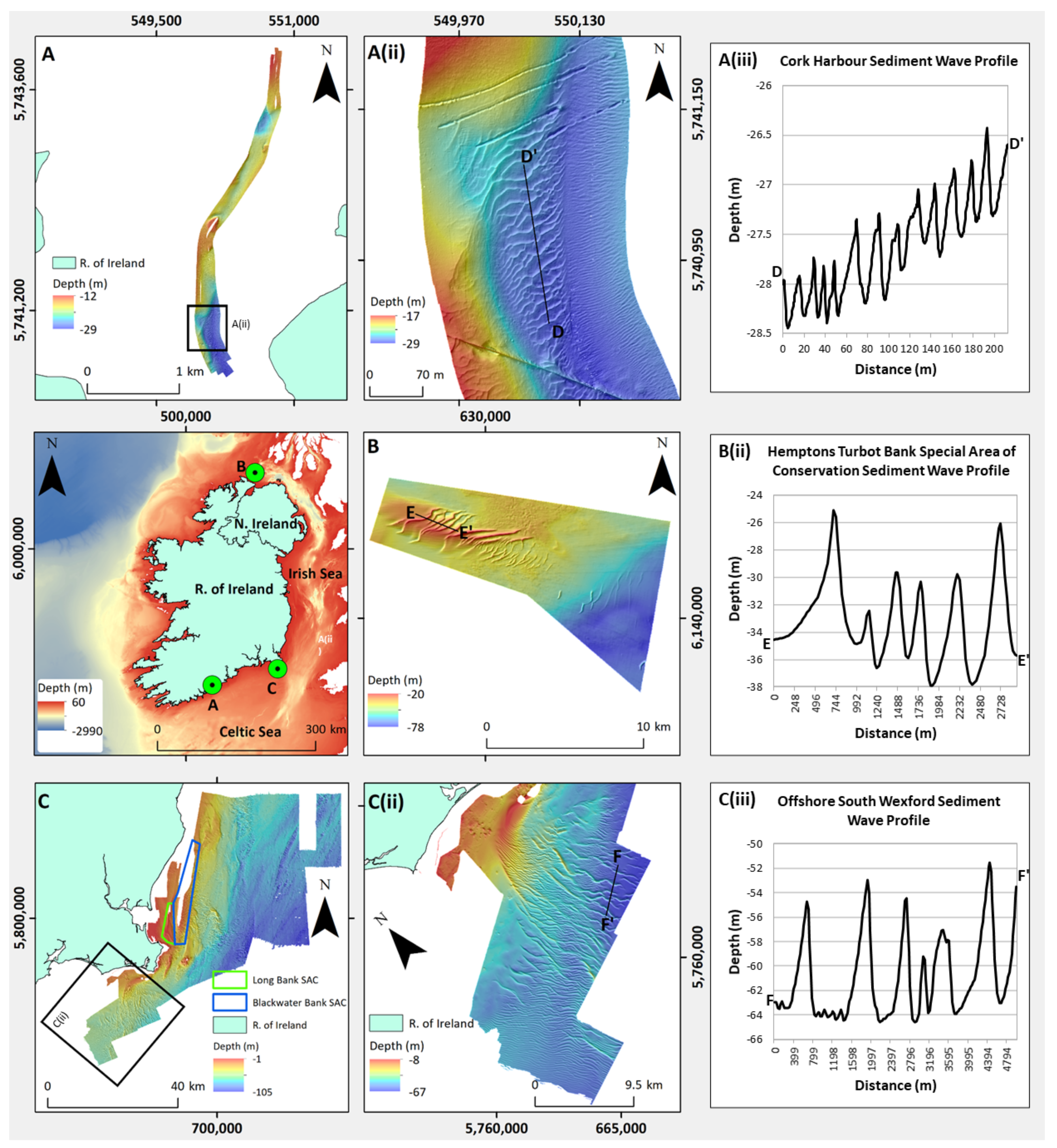
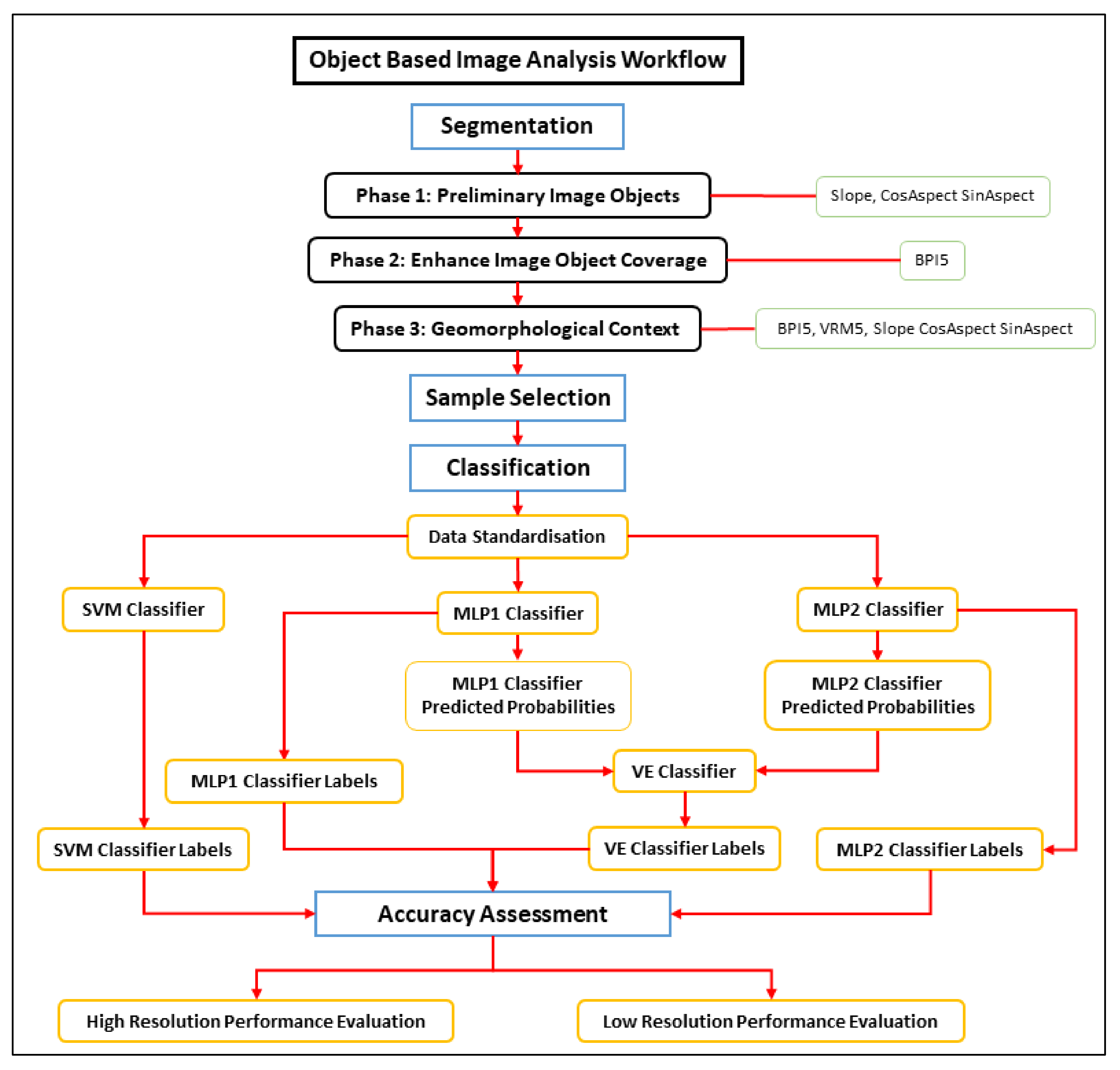
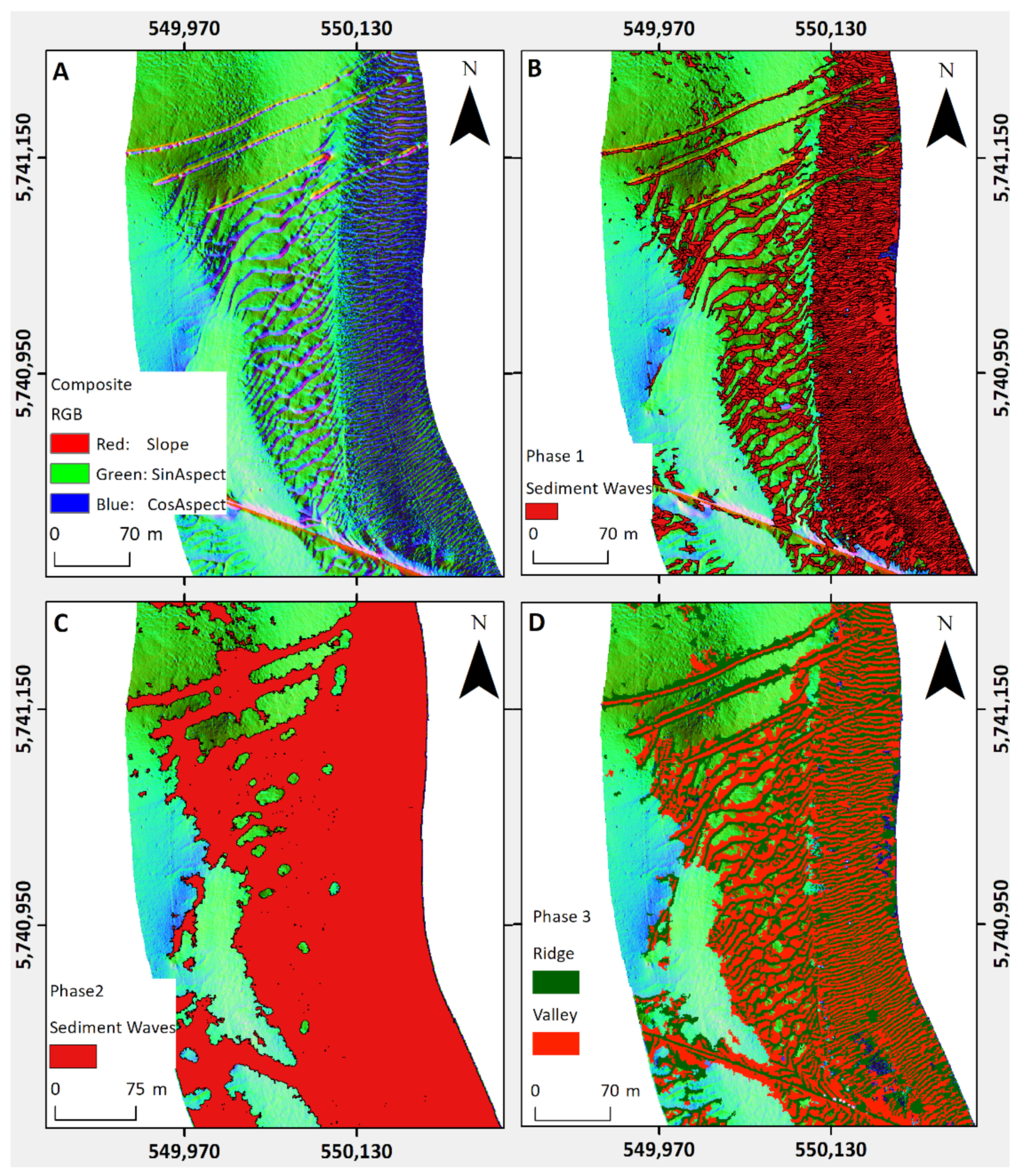
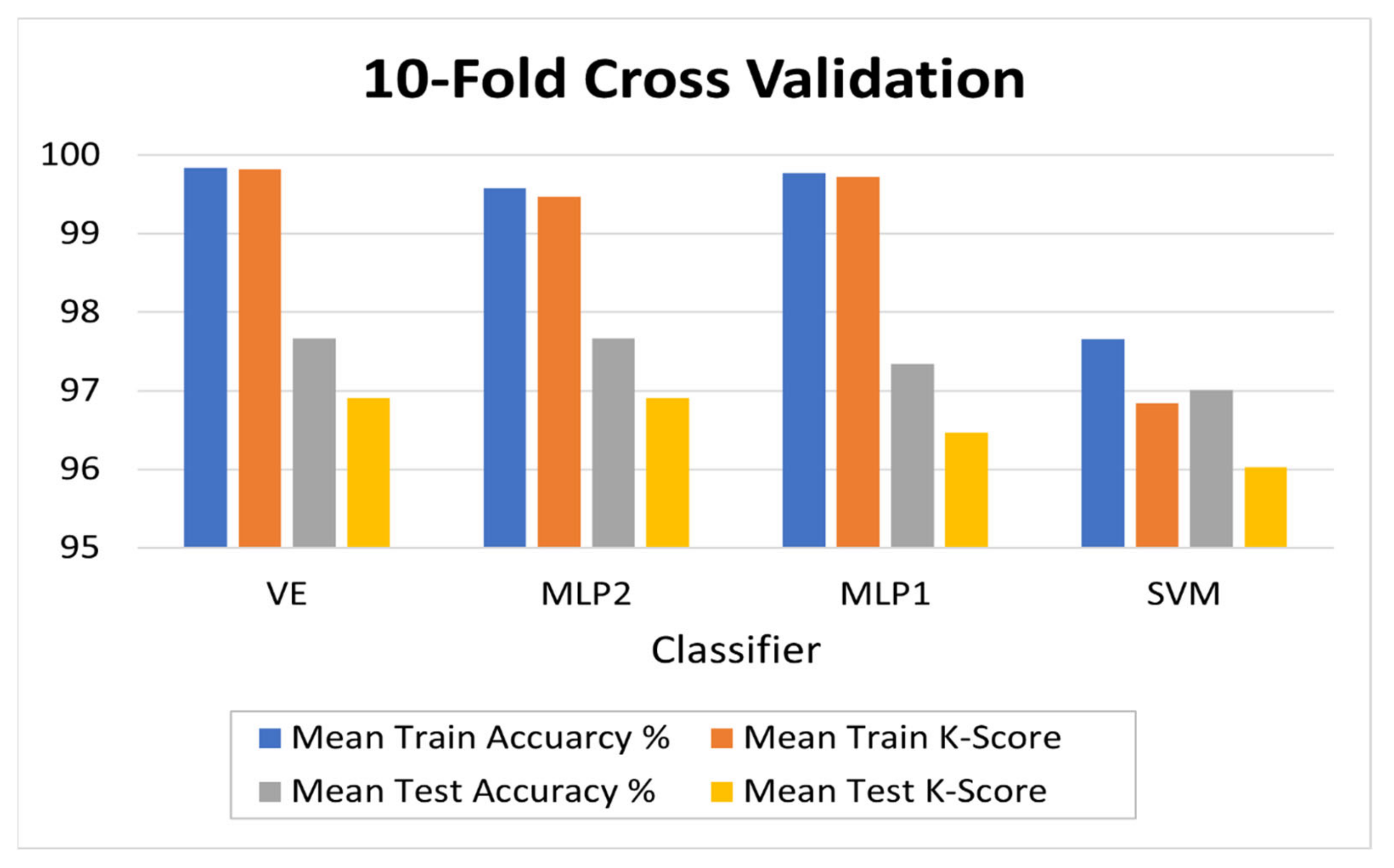
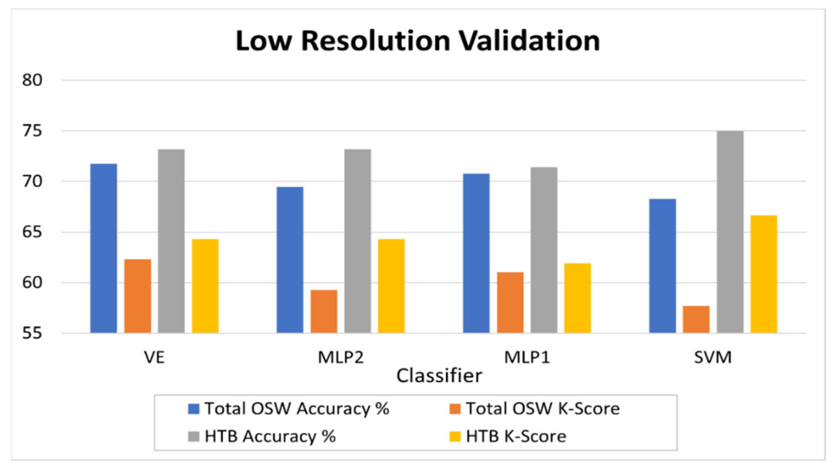
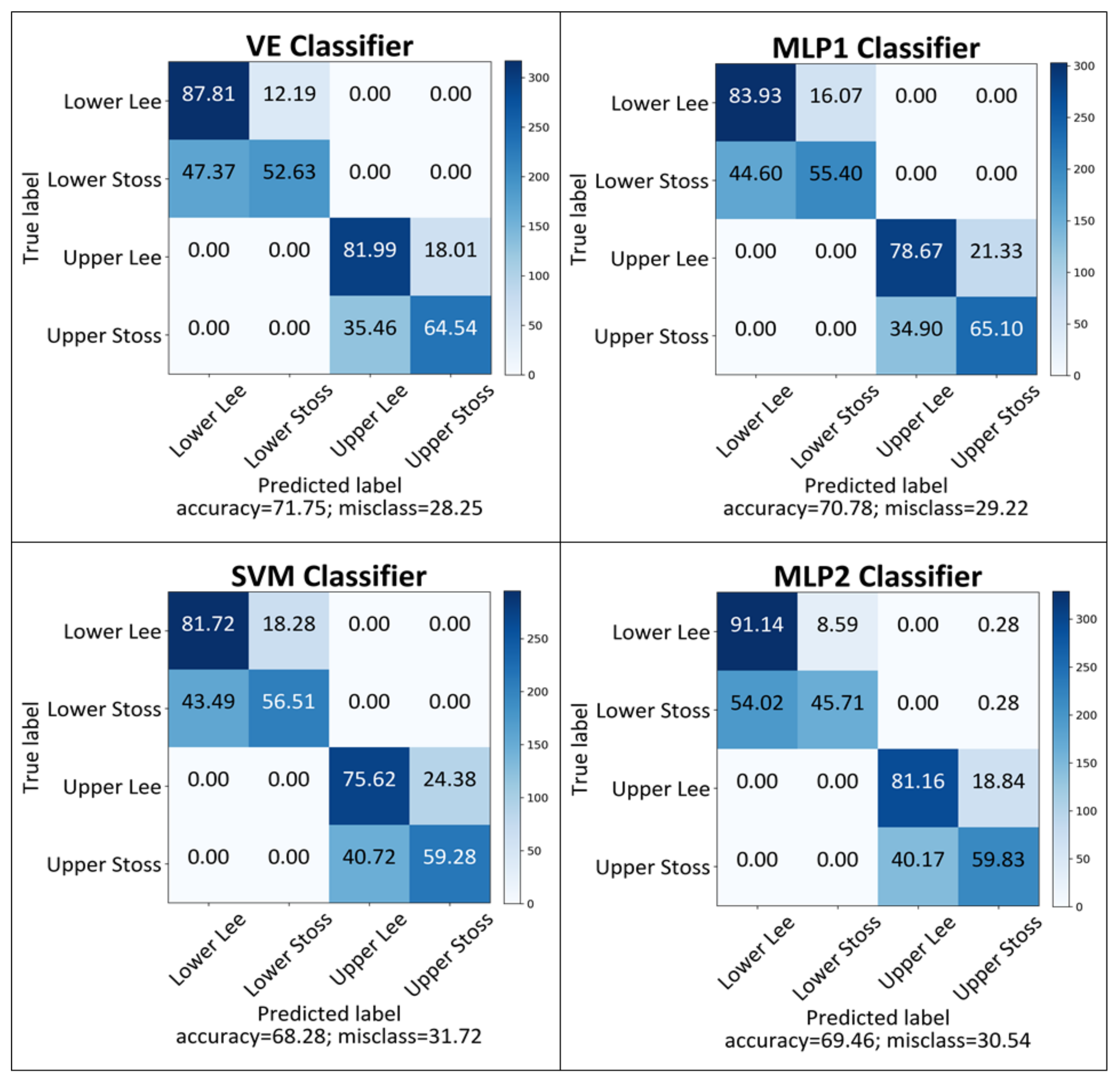
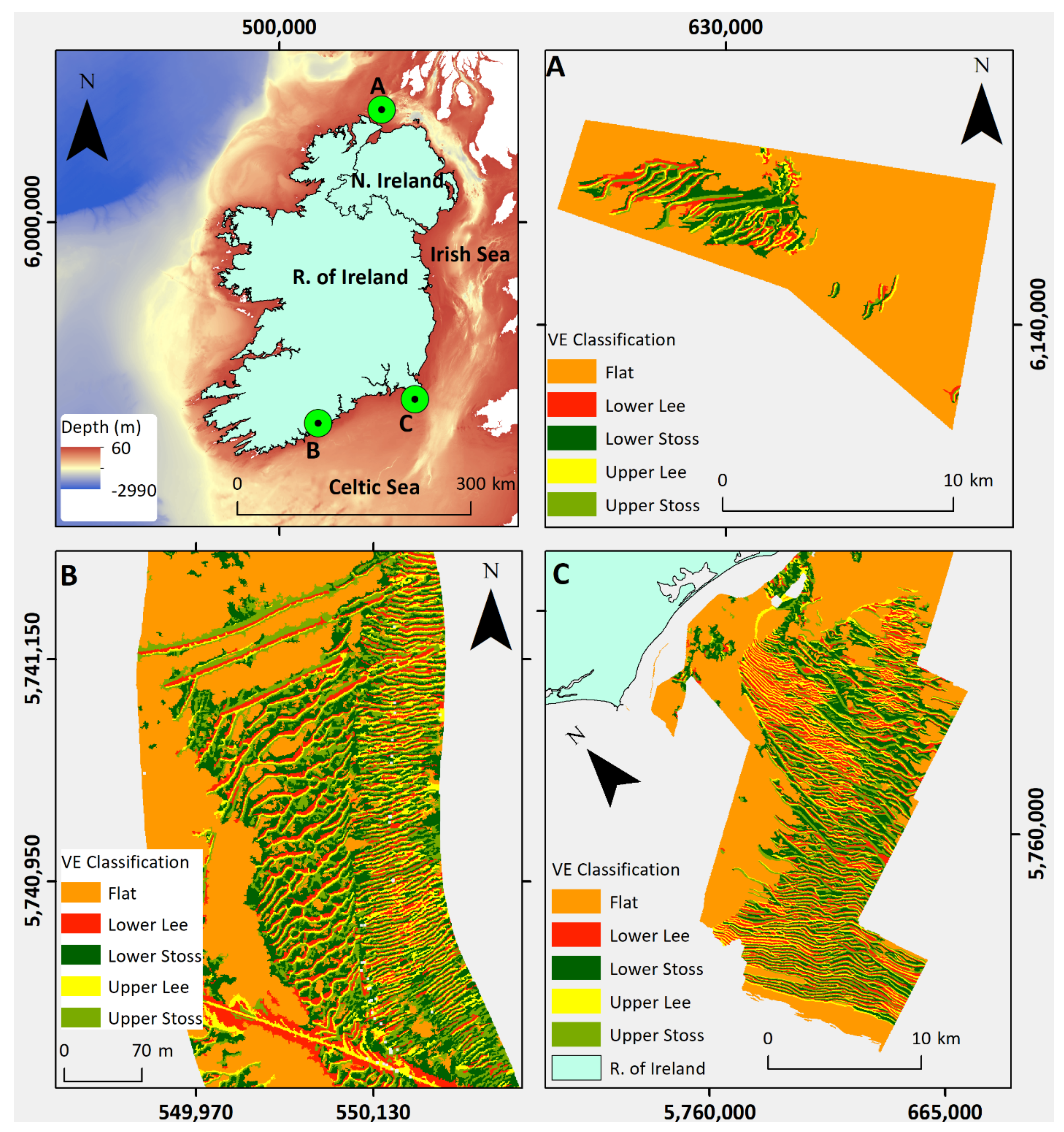
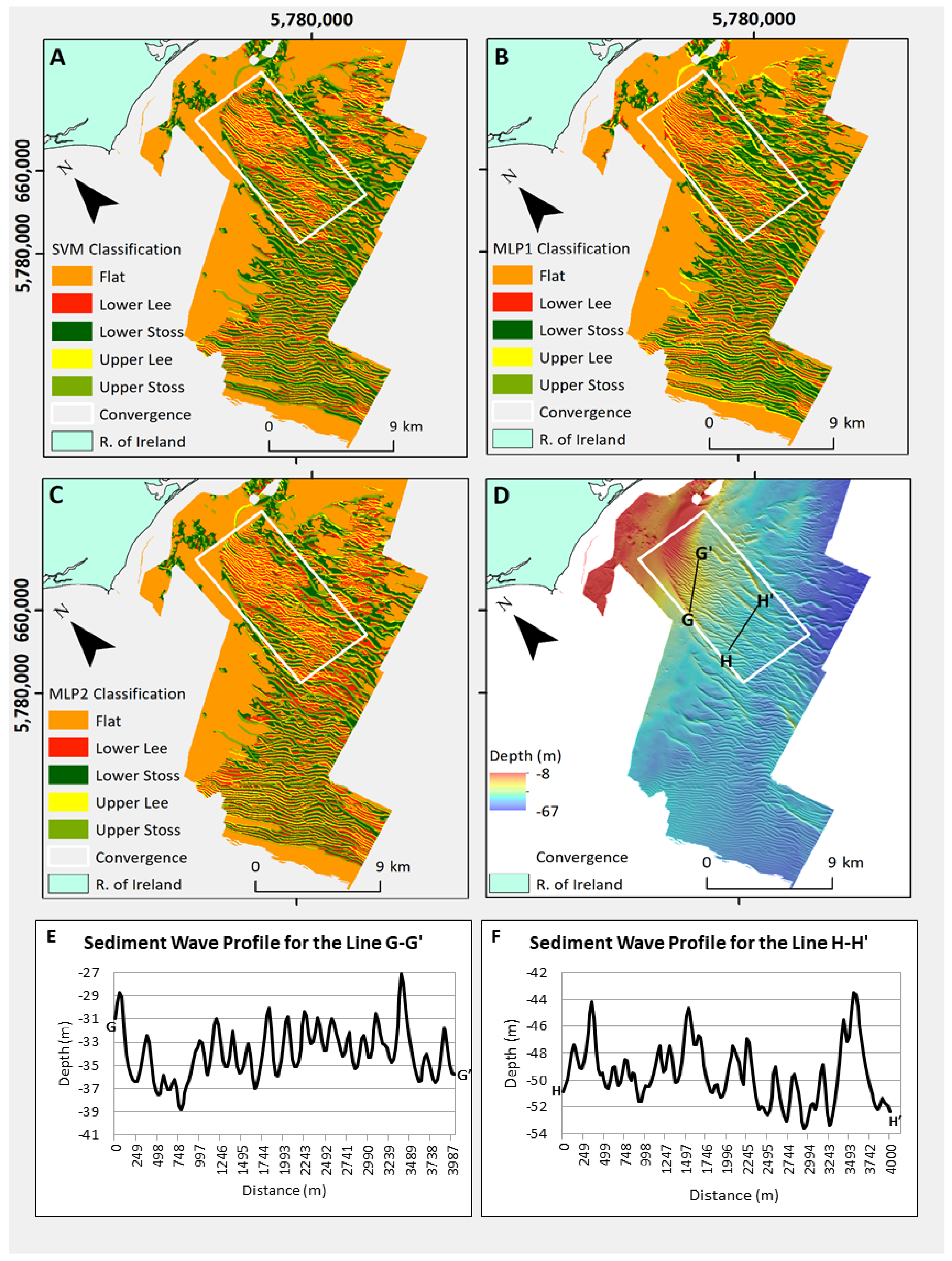
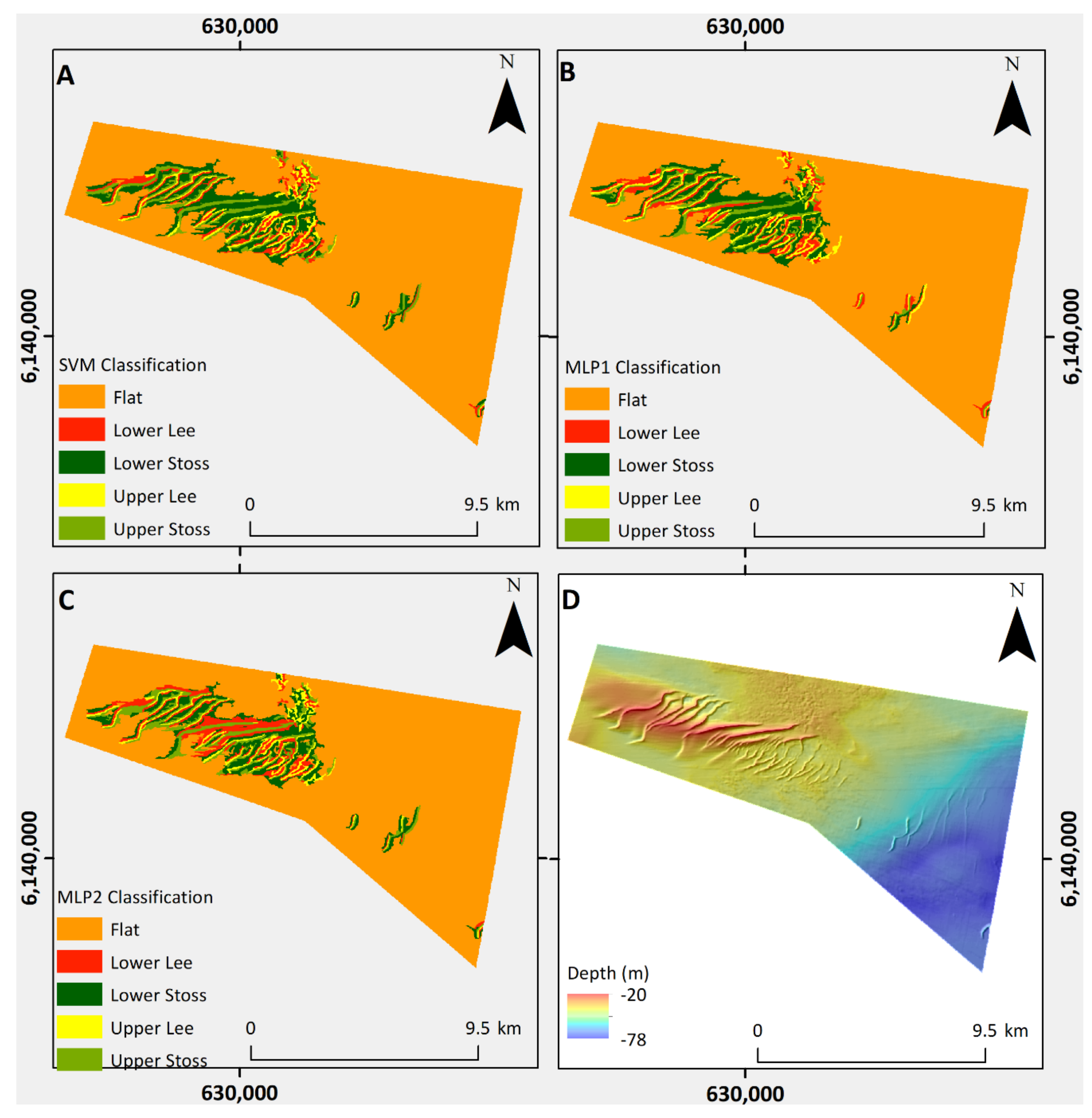
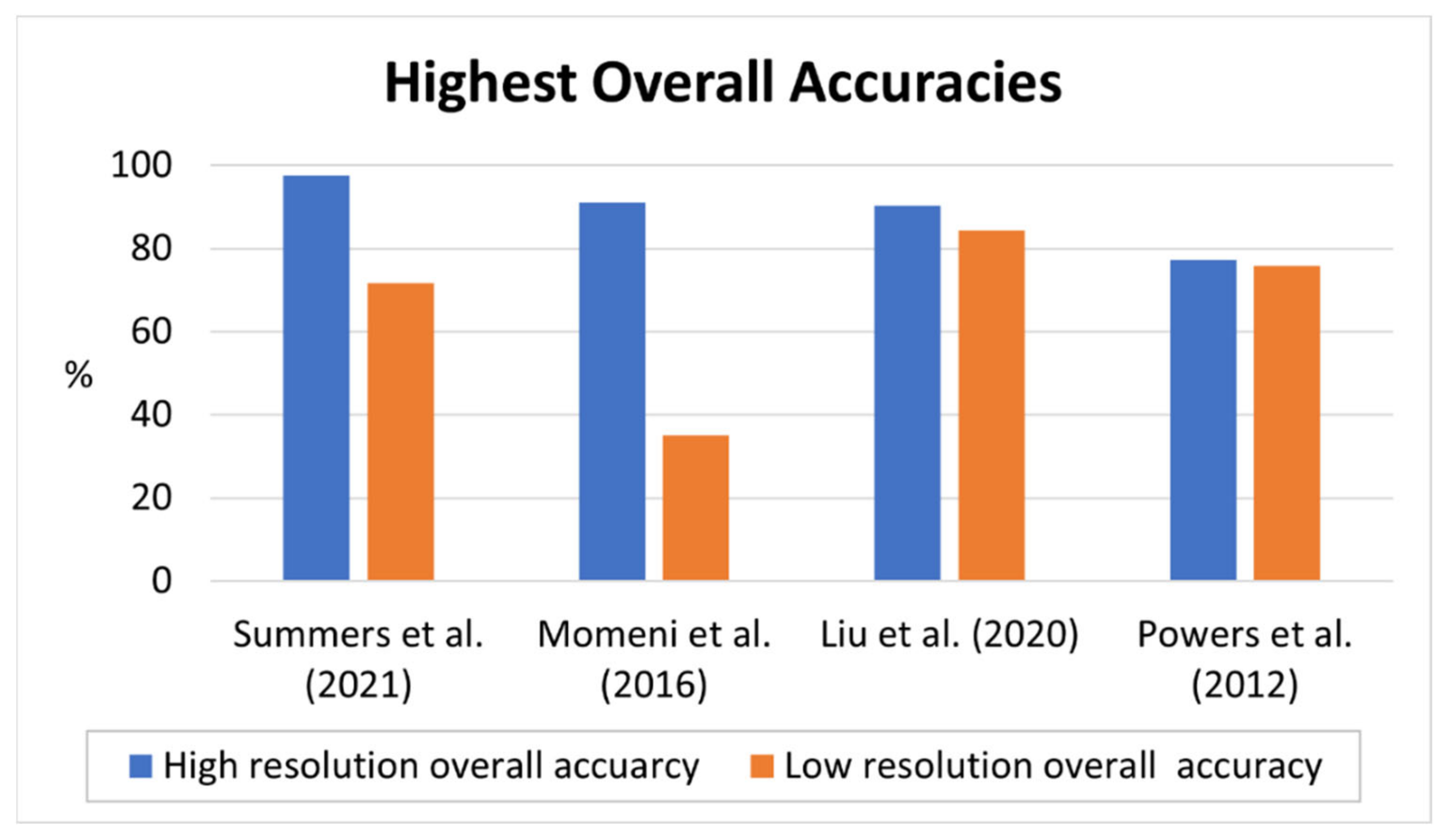
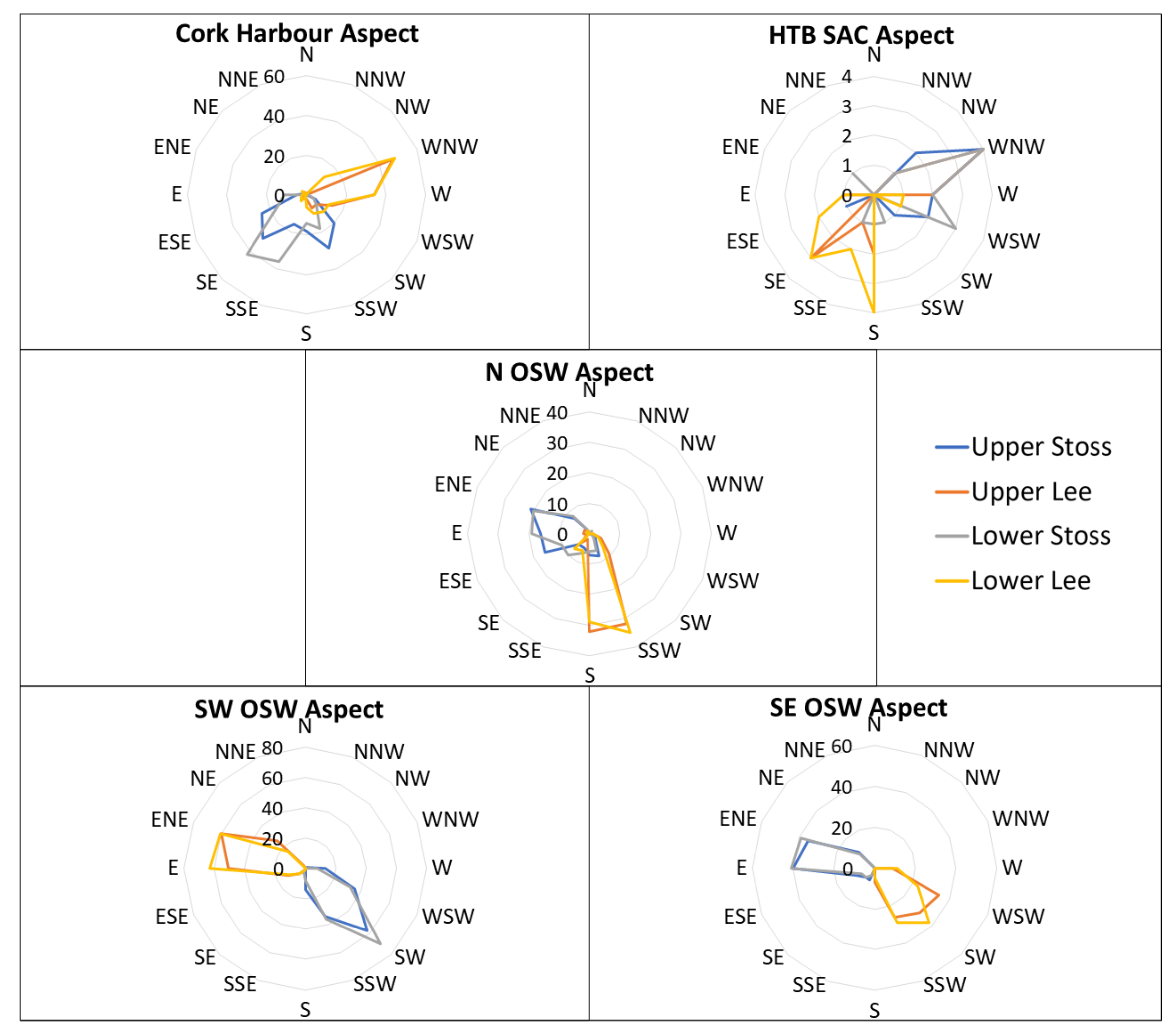
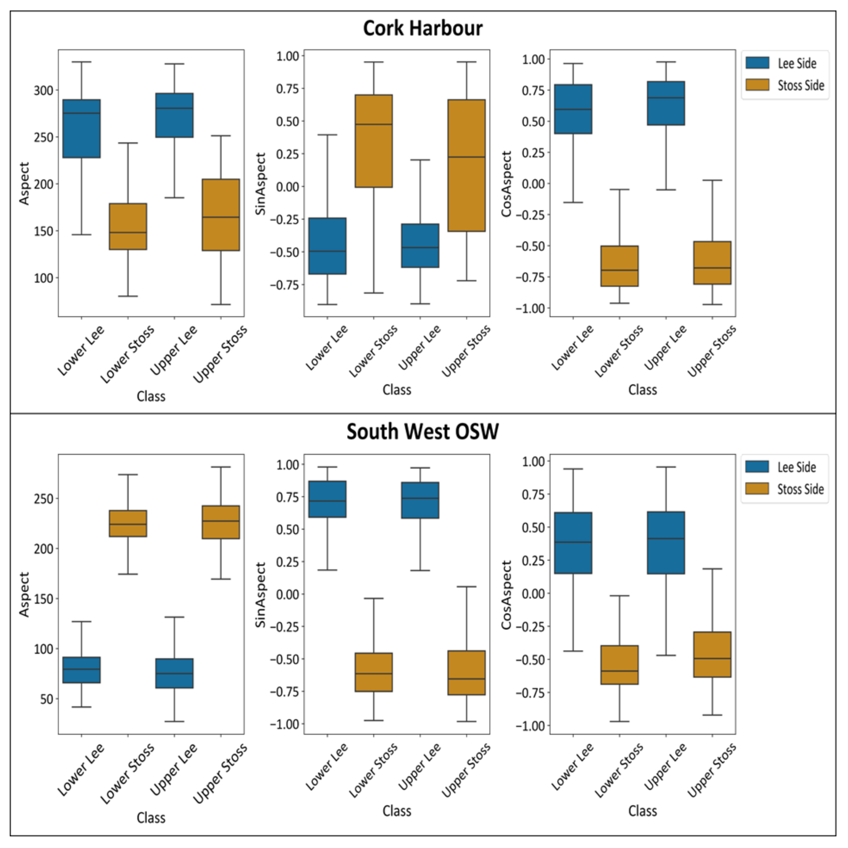
Table 1.
Datasets acquired from the EMODnet bathymetry data portal, including the original name of each file as designated on the EMODnet bathymetry data portal [53].
Table 1.
Datasets acquired from the EMODnet bathymetry data portal, including the original name of each file as designated on the EMODnet bathymetry data portal [53].
| EMODnet Dataset Name | Corresponding Region | Resolution (m) |
|---|---|---|
| CV16 CelticSeaIreland 14 m | South–West Offshore South Wexford (OSW) | 25 |
| HRDTM IrishSeaWexford 14 m | North–East OSW | 25 |
| 366_NorthAtlanticOceanDonegal | Hemptons Turbot Bank Special Area of Conservation (HTB SAC) | 25 |
Table 2.
Bathymetric derivatives extracted at each site. * Variable directly used in the segmentation process.
Table 2.
Bathymetric derivatives extracted at each site. * Variable directly used in the segmentation process.
| Bathymetric Derivatives | Scale (Pixel) |
|---|---|
| Aspect | 3 |
| Bathymetric Position Index (BPI) * | 3, 5 *, 9, 25 |
| CosAspect (Northness) * | 3 |
| Curvature | 3 |
| Planiform Curvature | 3 |
| Profile Curvature | 3 |
| Relative Topographic Position (RTP) | 3 |
| SinAspect (Eastness) * | 3 |
| Slope * | 3 |
| Vector Terrain Ruggedness (VRM) * | 3, 5 *, 9, 25 |
| Zeromean | 3, 9 |
Table 3.
Cross-validation summary scores across all 10 folds.
| Model | Statistic | Train Acc Score | Test Acc Score | Acc Score Diff | Train K-Score | Test K-Score | K-Score Diff |
|---|---|---|---|---|---|---|---|
| SVM | Mean | 97.66 | 97.01 | 1.57 | 96.84 | 96.03 | 2.10 |
| St Dev | 0.25 | 2.18 | 1.59 | 0.31 | 2.92 | 2.15 | |
| MLP2 | Mean | 99.58 | 97.67 | 2.23 | 99.47 | 96.91 | 2.98 |
| St Dev | 0.23 | 1.60 | 1.34 | 0.33 | 2.14 | 1.78 | |
| VE | Mean | 99.84 | 97.67 | 2.27 | 99.82 | 96.91 | 3.00 |
| St Dev | 0.21 | 1.60 | 1.50 | 0.24 | 2.14 | 2.03 | |
| MLP1 | Mean | 99.77 | 97.34 | 2.48 | 99.72 | 96.47 | 3.29 |
| St Dev | 0.34 | 1.39 | 1.37 | 0.43 | 1.87 | 1.84 |
Table 4.
The accuracy and K-scores for each of the North OSW (N OSW), the South–East OSW (SE OSW), and the South–West OSW (SW OSW) subset sites.
Table 4.
The accuracy and K-scores for each of the North OSW (N OSW), the South–East OSW (SE OSW), and the South–West OSW (SW OSW) subset sites.
| Study Site | North OSW | South–East OSW | South–West OSW |
|---|---|---|---|
| VE Accuracy (%) | 66.48 | 67.06 | 76.43 |
| VE K-score | 0.55 | 0.56 | 0.69 |
| MLP1 Accuracy (%) | 65.66 | 67.99 | 74.52 |
| MLP1 K-score | 0.54 | 0.57 | 0.66 |
| MLP2 Accuracy (%) | 65.11 | 62.62 | 75.48 |
| MLP2 K-score | 0.53 | 0.50 | 0.67 |
| SVM Accuracy (%) | 62.36 | 65.89 | 73.25 |
| SVM K-score | 0.50 | 0.55 | 0.64 |
Publisher’s Note: MDPI stays neutral with regard to jurisdictional claims in published maps and institutional affiliations. |
© 2021 by the authors. Licensee MDPI, Basel, Switzerland. This article is an open access article distributed under the terms and conditions of the Creative Commons Attribution (CC BY) license (https://creativecommons.org/licenses/by/4.0/).
Share and Cite
MDPI and ACS Style
Summers, G.; Lim, A.; Wheeler, A.J. A Scalable, Supervised Classification of Seabed Sediment Waves Using an Object-Based Image Analysis Approach. Remote Sens. 2021, 13, 2317. https://0-doi-org.brum.beds.ac.uk/10.3390/rs13122317
AMA Style
Summers G, Lim A, Wheeler AJ. A Scalable, Supervised Classification of Seabed Sediment Waves Using an Object-Based Image Analysis Approach. Remote Sensing. 2021; 13(12):2317. https://0-doi-org.brum.beds.ac.uk/10.3390/rs13122317
Chicago/Turabian StyleSummers, Gerard, Aaron Lim, and Andrew J. Wheeler. 2021. "A Scalable, Supervised Classification of Seabed Sediment Waves Using an Object-Based Image Analysis Approach" Remote Sensing 13, no. 12: 2317. https://0-doi-org.brum.beds.ac.uk/10.3390/rs13122317
Note that from the first issue of 2016, this journal uses article numbers instead of page numbers. See further details here.