Progressive Structure from Motion by Iteratively Prioritizing and Refining Match Pairs

Abstract

Structure from motion (SfM) has been treated as a mature technique to carry out the task of image orientation and 3D reconstruction. However, it is an ongoing challenge to obtain correct reconstruction results from image sets consisting of problematic match pairs. This paper investigated two types of problematic match pairs, stemming from repetitive structures and very short baselines. We built a weighted view-graph based on all potential match pairs and propose a progressive SfM method (PRMP-PSfM) that iteratively prioritizes and refines its match pairs (or edges). The method has two main steps: initialization and expansion. Initialization is developed for reliable seed reconstruction. Specifically, we prioritize a subset of match pairs by the union of multiple independent minimum spanning trees and refine them by the idea of cycle consistency inference (CCI), which aims to infer incorrect edges by analyzing the geometric consistency over cycles of the view-graph. The seed reconstruction is progressively expanded by iteratively adding new minimum spanning trees and refining the corresponding match pairs, and the expansion terminates when a certain completeness of the block is achieved. Results from evaluations on several public datasets demonstrate that PRMP-PSfM can successfully accomplish the image orientation task for datasets with repetitive structures and very short baselines and can obtain better or similar accuracy of reconstruction results compared to several state-of-the-art incremental and hierarchical SfM methods.

1. Introduction

Structure from motion (SfM) can automatically reconstruct sparse 3D points and estimate camera poses (also known as image orientation) from a set of 2D images, and has been extensively employed in photogrammetry [1,2]. Most feature-based SfM methods contain modules such as for feature extraction and matching [3], geometric verification [4,5,6], view-graph construction of match pairs [7,8,9], initial camera pose estimation [10,11,12], triangulation [13], and bundle adjustment [2,13,14]. Vertices in a view-graph denote images, and edges denote match pairs, which indicate a set of mutually overlapped image pairs. Taking the view-graph as an input, subsequent modules are used for image orientation tasks. According to the strategy of utilizing the view-graph, SfM can be categorized as incremental, hierarchical, or global.

Incremental SfM [10,12,15] typically starts with an initial reconstruction of a match pair or triplet and sequentially adds new images to the block. As the block grows, bundle adjustment is repeatedly conducted to refine the reconstruction results, which makes it time-consuming. While the efficacy of incremental methods has been widely demonstrated, they may have limitations in the presence of outliers in match pairs. First, the two-view reconstruction of the initial match pair is crucial, because the robustness and accuracy of the final reconstruction result relies heavily on it. Second, block growing is sensitive to the order of added new images. If a block grows in a wrong way, e.g., visually drifts of the newly oriented images arise, the whole reconstruction may be incorrectly estimated. This can occur, for example, due to the incorrect match pair of a repetitive structure, which typically causes ambiguities when finding the correct order. Third, triangulation to estimate 3D points suffers from limited robustness on match pairs stemming from very short baselines. Based on incremental methods, hierarchical SfM [16,17,18,19] creates atomic reconstructions in a divide-and-conquer manner and combines them hierarchically. While efficient due to the parallelization of dealing with atomic reconstructions, it is sensitive to the method by which these reconstructions grow. Global SfM [11,20,21] simultaneously considers all images to obtain consistent image orientation results. It is of high efficiency but is sensitive to outliers in match pairs. Recent developments of SfM focus on large-scale image sets, such as internet photo collections [21,22,23] and UAV image sets [18,24]. They typically consider moderate match pairs and pay less attention to those due to repetitive structures [8,25,26] and very short baselines [27,28,29]. These problematic match pairs can degrade SfM reconstruction results, or even lead to failure. We propose an SfM method to obtain correct reconstruction results for image sets with problematic match pairs stemming from repetitive structures and very short baselines.

Before detailing our contributions, we shortly review the state of the art of those related methods. Many strategies have been tried to cope with problematic match pairs [8,26,27,28,29,30,31]. It has been suggested to find a reliable subset of match pairs before executing image orientation [8,9,28]. This strategy is known as refining match pairs (or view-graph filtering [9]), which is equivalent to obtaining a robust subgraph from the original view-graph. RANSAC was used to delete inconsistent edges, randomly sampling spanning trees, generating cycles by walking two edges in the tree and one edge in the remaining set, deleting edges that lead to large discrepancies on rotation over cycles, and keeping the solution with the largest number of edges [20]. A Bayesian framework was designed to infer incorrect edges based on the inconsistency over cycles, which we call cycle consistency inference (CCI) [32]. Consistency was checked by chaining relative transformations to find erroneous image triplets and eliminating all match pairs among these at once [33]. These last three schemes considered only inconsistency using rotation that might not be able to find unreliable match pairs if image sets were captured by nearly pure translation motion. Verification was performed on both rotation and translation for every triplet in the view-graph, eliminating edges that could not pass [34]. 3D relative translations of all match pairs were projected in multiple 1D directions, eliminating match pairs whose relative translations stood out in the majority of directions [21]. However, the paper’s authors acknowledged that the this method fails to deal with match pairs due to repetitive structures [21,26]. Criteria were designed to indicate the probability of a match pair due to repetitive structure and a very short baseline [26]. The criterion on the repetitive structure was based on the assumption that match pairs overlap by a nearly constant amount, making it less general. The problem of the repetitive structure was addressed by prioritizing edges in one so-called verified maximum spanning tree and extending it to a sufficiently redundant view-graph [9].

Two strategies can be employed to improve the time efficiency and robustness of incremental SfM in the manipulation of the view-graph. First, view-graph partition and merging are typically used in hierarchical SfM. The idea was to divide the view-graph into a number of overlapping sub-graphs, each solved independently to create atomic reconstructions, and hierarchically merging these to obtain a complete reconstruction. To ensure accurate reconstruction, match pairs shared in different sub-graphs should be sufficiently redundant for reliable merging [24]. Thus, the quality of these shared match pairs has a significant influence on the merging process, and outliers might cause large drifts. A graph-based method for building reliable overlapping relations of images [29] was proposed to improve a previous hierarchical merging approach [16] in the presence of very short baselines and wide baselines (Wide baselines typically occur when terrestrial and UAV images are connected, and can lead to inaccurate SfM reconstruction results [29]). Second, the progressive scheme on the view-graph allows SfM to be carried out by iteratively prioritizing a subset of edges or match pairs, a strategy known as prioritizing match pairs. One maximum spanning tree was extracted from the view-graph to select the match pairs with the highest weights, which were used for an initial reconstruction, and expanded until no new images were added to the block among three consecutive iterations, implying that the block is completely built [35], alleviating the negative influence of some outliers in match pairs by carefully selecting the edges of the view-graph. However, a single tree is insufficiently robust if outliers are contained [9]; thus, it is dangerous to directly feed them into SfM pipelines, especially with a repetitive structure and very short baselines. A skeletal subset—not the full view-graph—was utilized to improve efficiency by up to an order of magnitude or more, with little or no loss in accuracy [36].

Based on an incremental method [10], termed COLMAP, we propose a progressive SfM pipeline (PRMP-PSfM) to obtain robust and accurate SfM reconstruction results. The remainder of this paper is organized as follows. Section 2 introduces COLMAP and discusses its limitations in the presence of a repetitive structure and very short baselines. Section 3 presents the proposed method, including initialization, which focuses on accurate seed reconstruction, and expansion, which yields a complete reconstruction result by progressively adding match pairs and corresponding images. Section 4 demonstrates the performance of our method on various image datasets. Some important components and settings of our method are discussed in Section 5. Section 6 concludes our work.

2. Incremental SfM Pipeline

2.1. COLMAP

Figure 1 depicts the workflow of the incremental SfM method (COLMAP), which is the basis of PRMP-PSfM. Given a set of images, feature extraction and matching (e.g., SIFT and nearest neighbor ratio matching [3]) are carried out to obtain all possible relations of images and corresponding conjugate points. These image pairs are verified by a two-view epipolar geometric constraint, i.e., geometric verification, which usually employs a five- [5] or eight-point method [4] with RANSAC [6] to yield all potential match pairs. They can be represented by a view-graph, where red vertices indicate images and gray edges indicate corresponding match pairs. Two-view reconstruction is initially built in the following estimation pipeline, and the next-best view selection and image registration orientate candidate images. Tracks are updated by concatenating the correspondences of match pairs, and track triangulation generates new 3D points to expand the reconstruction, which is refined by bundle adjustment. Outlier filtering eliminates inaccurate 3D points with large reprojection errors and images whose camera poses cause refinement to fail. The procedures of block growing, including next-best view selection, image registration, track triangulation, bundle adjustment, and outlier filtering, are repeated to obtain the final reconstruction result; red triangles in Figure 1 denote the estimated camera poses (i.e., image orientation parameters).

2.2. The Negative Influence of Problematic Match Pairs

Although many outliers in match pairs can be eliminated by RANSAC, some problematic match pairs still exist in the case of a repetitive structure or very short baselines. We take COLMAP (Figure 1) as an example of a conventional incremental SfM method and study its limitations in these instances.

2.2.1. Repetitive Structure

A repetitive structure in a human-made environment often yields ambiguities in pairwise image matching, e.g., wrong match pairs that observe similar but different objects, such as rows of windows and similar building facades. Many suspicious correspondences can be generated due to very similar descriptors, and some can pass epipolar geometric verification. Consequently, a repetitive structure typically results in wrong match pairs [26]. Figure 2 shows an example of a dataset with a repetitive structure. Images were captured along a closed loop of one cup whose front and back sides are symmetric. Figure 2a shows a correct match pair whose images view the same area, and Figure 2b shows a wrong match pair due to a repetitive structure. We represent all potential match pairs by a view-graph (Figure 2c), and insert it in COLMAP to obtain the SfM reconstruction result (Figure 2d). To make a comparison, we manually select the correct match pairs, yielding the filtered view-graph in Figure 2e, and generate a more reasonable reconstruction in Figure 2f. Investigating these two reconstruction results, the one from the original view-graph is a folded scene with large drifts of camera poses. This implies that wrong match pairs due to a repetitive structure can indeed have a negative impact on the reconstruction result. COLMAP adds candidate images with more visible 3D points and a more uniform distribution of correspondences, reflecting the inherent assumption that the match pairs are correctly overlapped. However, this assumption is sometimes invalid due to ambiguities caused by a repetitive structure. Once the block grows in a wrong way, it yields an incorrect reconstruction result, such as the folded scene in Figure 2d.

2.2.2. Very Short Baselines

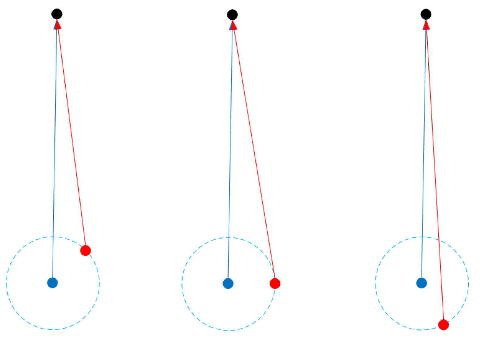
Very short baselines arise when the distance between images is insufficient or extremely close to pure rotation motion. Figure 3 shows two images (blue and red points) and one 3D point (a black point), which is the intersection point of two view rays (blue and red arrows). When we keep one image (blue) and the 3D point (back) fixed, and move the another image (red) along a circle (dotted line) with the center of the blue point with a constant radius, different cases of two-view intersection can be observed. If the radius is very small, i.e., with a very short baseline between these two images, it leads to a small intersection angle. Such poor intersection geometry typically results in an ill-posed problem of estimating coordinated 3D points [13,26,27].

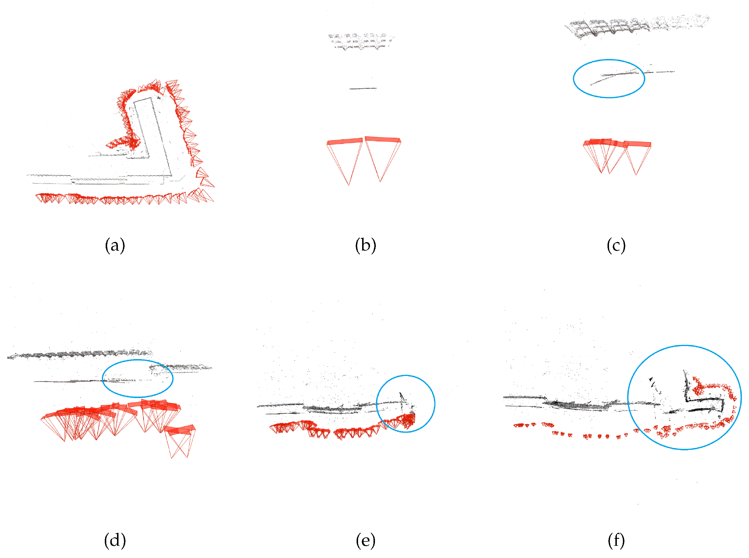
To illustrate the influence on SfM results, we tested a dataset with very short baselines in COLMAP; corresponding reconstruction results are shown in Figure 4. The reference reconstruction result (Figure 4a) was obtained by only using correct match pairs. When both correct match pairs and ones with very short baselines were input, the reconstruction result becomes worse, as can be seen in Figure 4b–f. In comparison to the reference, it can be seen that COLMAP can obtain a good two-view reconstruction (Figure 4b), but shows increasing drifts of camera poses as the block grows. As Figure 4c shows, some inaccurate 3D points (blue ellipses) are generated in the expanded reconstruction, mainly due to corresponding match pairs with very short baselines. The final reconstruction result (Figure 4f) suffers from obvious visual drifts due to error accumulation.

3. Method

3.1. Overview

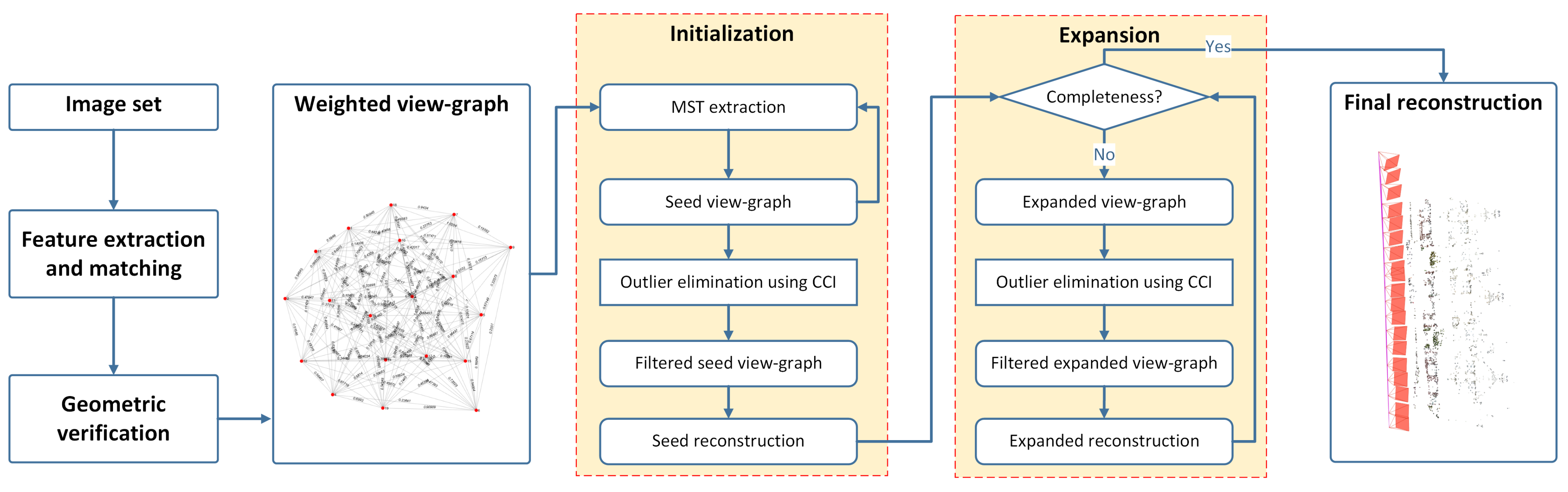
We present PRMP-PSfM, whose workflow is shown in Figure 5. The input is a set of images, following the procedures of COLMAP (Figure 1) to obtain all potential match pairs, from which we construct a weighted view-graph in Section 3.2. Weights of edges indicate the costs of match pairs; the smaller the weight, the more the possibility that a match pair is correct. The image orientation pipeline includes initialization and expansion. In initialization, we generate a seed view-graph comprising multiple independent minimum spanning trees (MSTs), containing subsets of match pairs with smaller costs, and apply outlier elimination using CCI for a filtered seed view-graph. We insert this robust view-graph in COLMAP to obtain an accurate reconstruction result, a procedure called seed reconstruction. Images are sometimes excluded from seed reconstruction due to the filtering procedure; expansion is designed to achieve a more complete reconstruction. Completeness is checked to decide whether the expansion is necessary. If this condition is met by the seed reconstruction, then we set it as the final reconstruction result. Otherwise, seed reconstruction is incomplete and expansion is carried out. New MSTs are progressively added to the filtered seed view-graph to realize a denser graph, i.e., an expanded view-graph, which is filtered by outlier elimination using CCI before applying incremental SfM. The procedure is repeated until completeness is achieved.

3.2. Construction of Weighted View-Graph

The undirected view-graph $G=(V,E)$ is often used to represent relations between images. Vertices V indicate images, and edges E indicate match pairs; $e_{ij}\in E$ means two images of vertices $\{v_i,v_j\}\in V$ are successfully matched after geometric verification. To prioritize the edges by MST, we need to construct a weighted view-graph $G=(V,E,W)$, where W is a set of scalar values indicating the costs of edges. The smaller the cost, the more likely it is that the edge is correct. It has been suggested to calculate the cost for each edge by Equation (1) [37], where M is the number of feature correspondences, and $\mathsf{\Theta }$ is the mean intersection angle of all correspondences; they are normalized to [0, 1] and balanced by a factor $\mu$, which is set by default to 0.1. After the costs of edges were calculated, one MST was extracted to select the most reliable match pairs. Only tracks generated from these selected match pairs were used in the proposed method, which yielded a robust method to avoid abundant or outlier tracks [37]. More feature correspondences of one match pair can generally produce a more robust estimate [8,9,37], which is also reasonable in the presence of repetitive structures because after geometric verification, the feature correspondences of a correctly overlapping match pair outnumber those of a match pair with a repetitive structure [9,35]. For very short baselines, which typically result in very small intersection angles, $\mathsf{\Theta }$ is a suitable criterion to indicate their lengths. Hence, we generate the weight view-graph as [37]

$$W=\frac{1}{M}+\mu \times \frac{1}{\mathsf{\Theta }}$$

(1)

3.3. Outlier Elimination Using CCI

We introduce a general outlier detection method, CCI [32], by analyzing the geometric consistencies over cycles. Given a view-graph (Figure 6a) and the estimated relative transformations $\left\{T_e\right\}$ of all potential match pairs, the exhaustive cycles of the length of all image triplets C are extracted (Figure 6b), and the deviation or inconsistency of each cycle is computed using a non-negative function $d\left(T_c\right)$, $c\in C$, where $T_c$ is the chained transformation along the cycle. If one cycle is ideally consistent, then $d\left(T_c\right)$ should equal zero, while noise or outliers in match pairs can lead to a nonzero value. If $d\left(T_c\right)$ exceeds a threshold, then at least one problematic match pair exists in the cycle. Based on this idea, a Bayesian inference framework was proposed [32]. Define the following:

$P(d\left(T_c\right)\mid x_c=1)$: probability of deviation $d\left(T_c\right)$ for a cycle, assuming all its edges are correct;

$P(d\left(T_c\right)\mid x_c=0)$: probability of deviation $d\left(T_c\right)$ for a cycle, assuming at least one edge in the cycle is incorrect;

$P\left(x_e\right)$: prior probability for indicating the quality of an edge.

Latent binary variables, $x_e$, $x_c$, are introduced for each edge and cycle, respectively, where $x_e=0$ indicates an incorrect edge, $x_e=1$ indicates a correct edge, and after chaining all the edges over a cycle, $x_c=\underset{e\in c}{min}{x}_e$. Hence, $x_c=1$ indicates all edges of the cycle are correct, and $x_c=0$ if at least one incorrect edge exists. $x_e\in \{0,1\}$ should be assigned to all edges to maximize the joint probability function:

$$\prod _{c\in C}P(x_{e\in c}\mid d\left(T_c\right))\propto \prod _{e}P\left(x_e\right)\prod _{c\in C}P(d\left(T_c\right)\mid x_c)$$

(2)

The inference problem can be represented by factor graphs and solved by loopy belief propagation [38]. Once the inference is finished, we determined a set of incorrect edges (dark lines in Figure 6c), i.e., $\{x_e=0\}$, and eliminate them to form a filtered view-graph, as seen in Figure 6d.

We elaborate on the calculation of the probability mode of cycles $P(d\left(T_c\right)\mid x_c=1)$. For image sets with known intrinsic parameters, we obtained the estimated relative orientations of match pairs by decomposing the essential matrix. These relative orientations have five degrees of freedom, including relative rotations and translations. For a cycle formed by three images i, j, k, when the estimated relative rotation matrices of image pairs $R_{ij}$, $R_{ik}$, $R_{jk}$ are known, we denote the chained rotation over the cycle as $c_R=R_{ij}{R}_{jk}{R}_{ik}^{\top }$, and the difference on rotation as $d_{\angle }\left(c_R\right)=arccos(\frac{\mathrm{trace}\left(c_R\right)-1}{2})$. Given the estimated relative translation vectors $t_{ij}$, $t_{ik}$, $t_{jk}$, the chained translation angle is $c_T={\theta }_i+{\theta }_j+{\theta }_k$, where angles ${\theta }_i$, ${\theta }_j$, ${\theta }_k$ for the images are, respectively, calculated, i.e., ${\theta }_i=arccos(\frac{t_{ij}^{\top }{t}_{ik}}{\parallel t_{ij}\parallel \parallel t_{ik}\parallel })$. We calculated the difference on translation $d_{\angle }\left(c_T\right)=\left|c_T-180°\right|$, where 180° is the sum of the interior intersection angles of this triangle (cycle of length three). We set the deviation as the larger of the two differences in Equation (3). We fit the inlier portions $\{d\left(T_c\right)\le \sqrt{\left|c\right|}\epsilon \}$ as an exponential distribution and empirically set $\epsilon$ to 2 degrees. $F(d\left(T_c\right);\lambda )$ is the cumulative distribution function, where $\lambda$ is the parameter of the exponential function, which is adaptively estimated from the inlier data. As inconsistent cycles may have small $d\left(T_c\right)$, e.g., when the error of one incorrect edge is offset by another, we limit the maximum value of $P(d\left(T_c\right)\mid x_c=1)$ in Equation (4) to 0.9 instead of to 1:

$$d\left(T_c\right)=max\left[d_{\angle }\left(c_R\right),d_{\angle }\left(c_T\right)\right]$$

(3)

$$P(d\left(T_c\right)\mid x_c=1)=\left\{\begin{array}{ccc}\hfill 0.9[1-F(d\left(T_c\right);\lambda )]& ,\hfill & \hfill d\left(T_c\right)\le \sqrt{\left|c\right|}\epsilon ,\\ \hfill 0& ,\hfill & \hfill d\left(T_c\right)>\sqrt{\left|c\right|}\epsilon .\end{array}\right.$$

(4)

3.4. Initialization

For good seed reconstruction, the input view-graph should be as accurate as possible. Most incremental methods [10,33] employ the original view-graph. As discussed in Section 2.2, problematic match pairs must be eliminated because they have a negative influence on the reconstruction results of the incremental SfM method. One MST can be used as the input view-graph [35]. However, it is difficult to guarantee that its edges are correct, especially for image sets with problematic match pairs. Images in one MST are only two-fold overlapping, and the redundancy of edges is insufficient for accurate seed reconstruction if a selected edge in the MST is not correct [9].

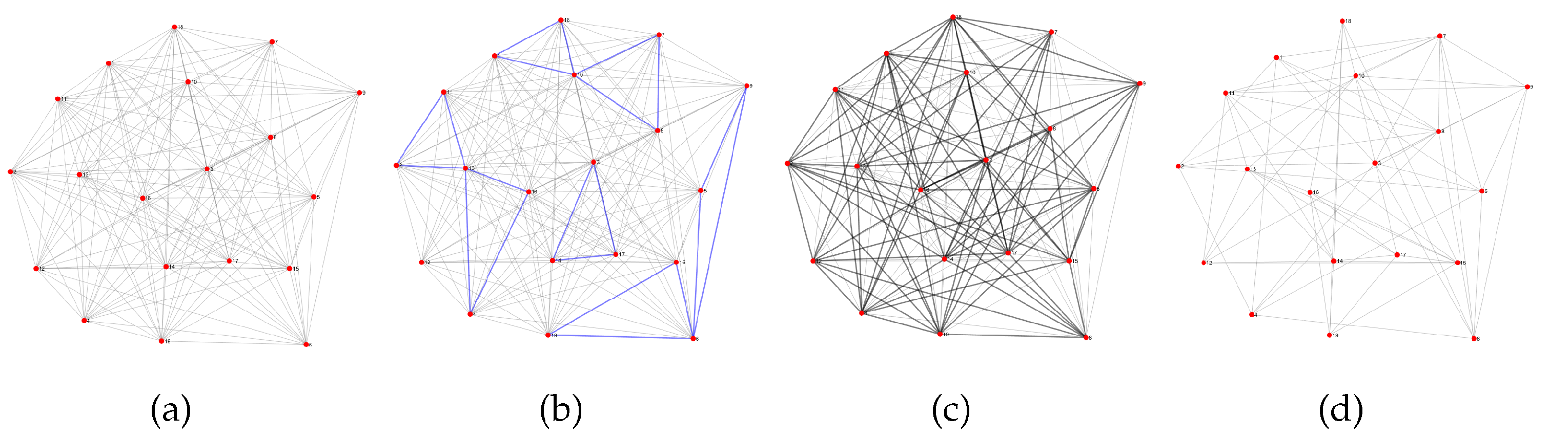
As Figure 5 shows, we generate the filtered seed view-graph considering both accuracy and redundancy of match pairs, as shown in Figure 7. Given the original view-graph (Figure 7a), a number of MSTs comprise the seed view-graph (Figure 7b), and a filtered one, the filtered seed view-graph (Figure 7c), is obtained by outlier elimination using CCI. Specifically, given the weighted view-graph $G=(V,E,W)$, the first MST is extracted [39], which contains all vertices of V and $\left|V\right|-1$ edges with the smallest costs, and these edges are removed from G, yielding a new graph $G^{\prime }$. Here, $\left|·\right|$ counts the number of vertices. The second MST is extracted from $G^{\prime }$, and this ensures there are no repeated edges between two MSTs, i.e., so-called orthogonal MSTs [25,35]. The above processes are repeated several times, and these extracted orthogonal MSTs compose a seed view-graph $G_{seed}$ with $N_{seed}$ iterations. With a smaller $N_{seed}$, the graph contains more accurate and less redundant edges, whereas a larger $N_{seed}$ makes for a denser graph that may contain some unreliable edges. We first compute the averaging degree for all vertices, $\Delta \left(G\right)$, which indicates the density of the original view-graph, and multiply by a factor $\alpha$ to determine $N_{seed}$ for adaptability:

$$\begin{array}{c}\hfill N_{seed}=\alpha \times \Delta \left(G\right)\\ \hfill \Delta \left(G\right)=\frac{{\sum }_{i=1}^{\left|V\right|}deg\left(v_i\right)}{\left|V\right|}\end{array}$$

(5)

where $deg\left(v_i\right)$ is the degree of vertex $v_i\in V$, i.e., the number of edges that are incident to it. Hence, our method is less sensitive to the density of view-graphs. CCI is then used to detect and eliminate outliers on $G_{seed}$ to yield a filtered seed view-graph $G_{seed}^f$. We employ the largest connected component (in graph theory, a connected component of an undirected graph is a subgraph in which any two vertices are connected to each other by paths, and which is connected to no additional vertices in the rest of the graph) of $G_{seed}^f$ for seed reconstruction. Note that some edges are possibly filtered out, which might cause $G_{seed}^f$ to be disconnected and lead to several individual reconstructions. Therefore, the biggest connected component is selected for seed reconstruction.

3.5. Expansion

Expansion aims to obtain a more complete reconstruction result. In general, when the block completely grows, complete reconstruction is reached; thus, regarding the condition of completeness, we suggest that all images in the input view-graph should be successfully orientated. Initialization uses the filtered seed view-graph with rather good match pairs to ensure accurate seed reconstruction. However, its completeness is not strictly guaranteed. Incomplete seed reconstruction might arise for two reasons: (1) the largest connected component of the filtered seed view-graph does not cover all images, yielding only part of the complete reconstruction result; (2) some unstable images are excluded by the procedure of outlier filtering (see Figure 1).

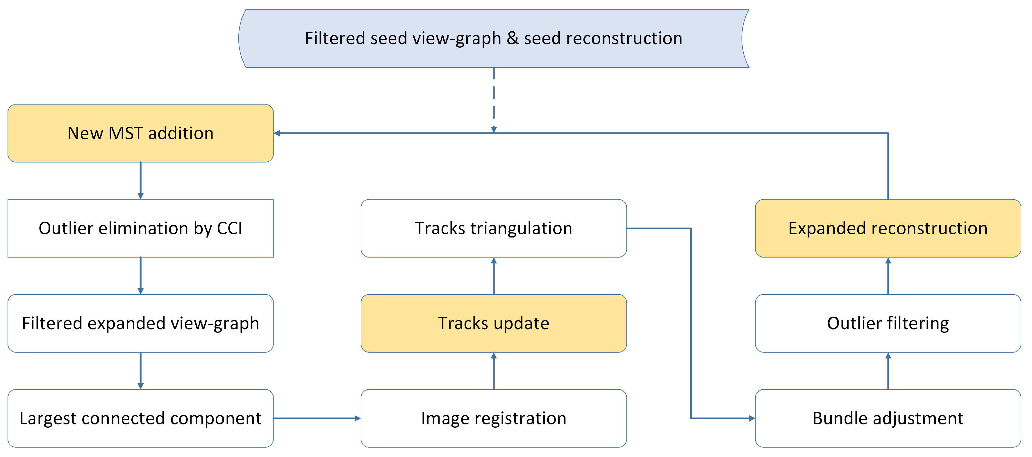
As Figure 5 shows, the condition of completeness is checked at the beginning of expansion. If the condition is reached, then the seed reconstruction is output as the final result. It is otherwise necessary to expand the seed reconstruction for completeness, and the filtered expanded view-graph and expanded reconstruction are similarly generated. A workflow is given in Figure 8. We progressively add new MSTs to the filtered seed view-graph to generate a denser graph. By conducting outlier elimination using CCI, we can obtain the filtered expanded view-graph. Analogously, we employ the largest connected component to add new edges and corresponding new images. Once these new images are orientated, the tracks are updated by concatenating the correspondences of match pairs of the current view-graph. Subsequent processes, as shown in Figure 1, are progressively conducted until the condition of completeness is reached.

4. Results

We quantitatively and qualitatively evaluated the efficacy of PRMP-PSfM at generating accurate SfM reconstruction results. Experiments were conducted on datasets with different types of problematic match pairs, including repetitive structures and very short baselines. PRMP-PSfM was then compared to several state-of-the-art SfM pipelines, including three incremental methods (COLMAP [10], (COLMAP software was downloaded from https://github.com/colmap/colmap/releases, version 3.6-dev.2 [released 24 March 2019]. All experiments were conducted with the settings suggested by [10]) VisualSFM [15], (VisualSFM software was downloaded from http://ccwu.me/vsfm/, version V0.5.26 [accessed September 2020]. All experiments were conducted with the default settings) and OpenMVG [33] (Code was downloaded from https://github.com/openMVG/openMVG, version v1.5 [released 16 July 2019]. We used its incremental SfM pipeline. Details can be found at https://openmvg.readthedocs.io/en/latest/)) and two hierarchical methods (GraphSfM [19] (Code was downloaded from https://github.com/AIBluefisher/EGSfM. The version provided by the original author was implemented based on OpenMVG) and APE [29] (Note that we were unable to obtain the APE source code. We referred to the results of the original paper for comparison)). APE integrates a series of processes of dealing with problematic match pairs due to wide baselines and very short baselines. Some processes of these methods used in the experiments are listed in

Table 1. Some properties of the methods used in our experiments: FE—feature extraction; FM—feature matching; MP—match pairs; BA—bundle adjustment; PRMP—prioritizing and refining match pairs; LM—Levenberg–Marquardt; PCG—preconditioned conjugate gradient; RBA—robust bundle adjustment. “Original” indicates that the original view-graph is taken as input and there is no specified process on its match pairs. “-” indicates that the corresponding items are unavailable.

Framework	FE	FM	MP	BA
PRMP-PSfM	SiftGPU [15]	Nearest neighbor ratio	PRMP	LM [14]
COLMAP	SiftGPU [15]	Nearest neighbor ratio	Original	LM [14]
VisualSFM	SiftGPU [15]	Preemptive feature matching [15]	Original	PCG [15]
OpenMVG	SIFT	Cascade hashing [40]	Original	LM [14]
GraphSfM	SIFT	Cascade hashing [40]	Original	LM [14]
APE	SiftGPU [15]	Wide baseline method [29]	Classification [29]	RBA [29]

. Considering that they are all complex systems, the processes related to the view-graph are mainly summarized. We set $\alpha =0.25$ for all experiments.

4.1. Datasets

Table 2. The description of image datasets used in our experiments.

Name	Images	Resolution	Type	Reference
Books	21	1067 × 800	Repetitive structure	Yes
Cereal	25
Cup	64
Desk	31
Street	19
Indoor	152	1200 × 800	Repetitive structure	No
Redmond	148	3968 × 2232
ToH	341	4368 × 2912
B1	182	3936 × 2624	Repetitive structure Very short baselines	Yes
B2	215
B3	342
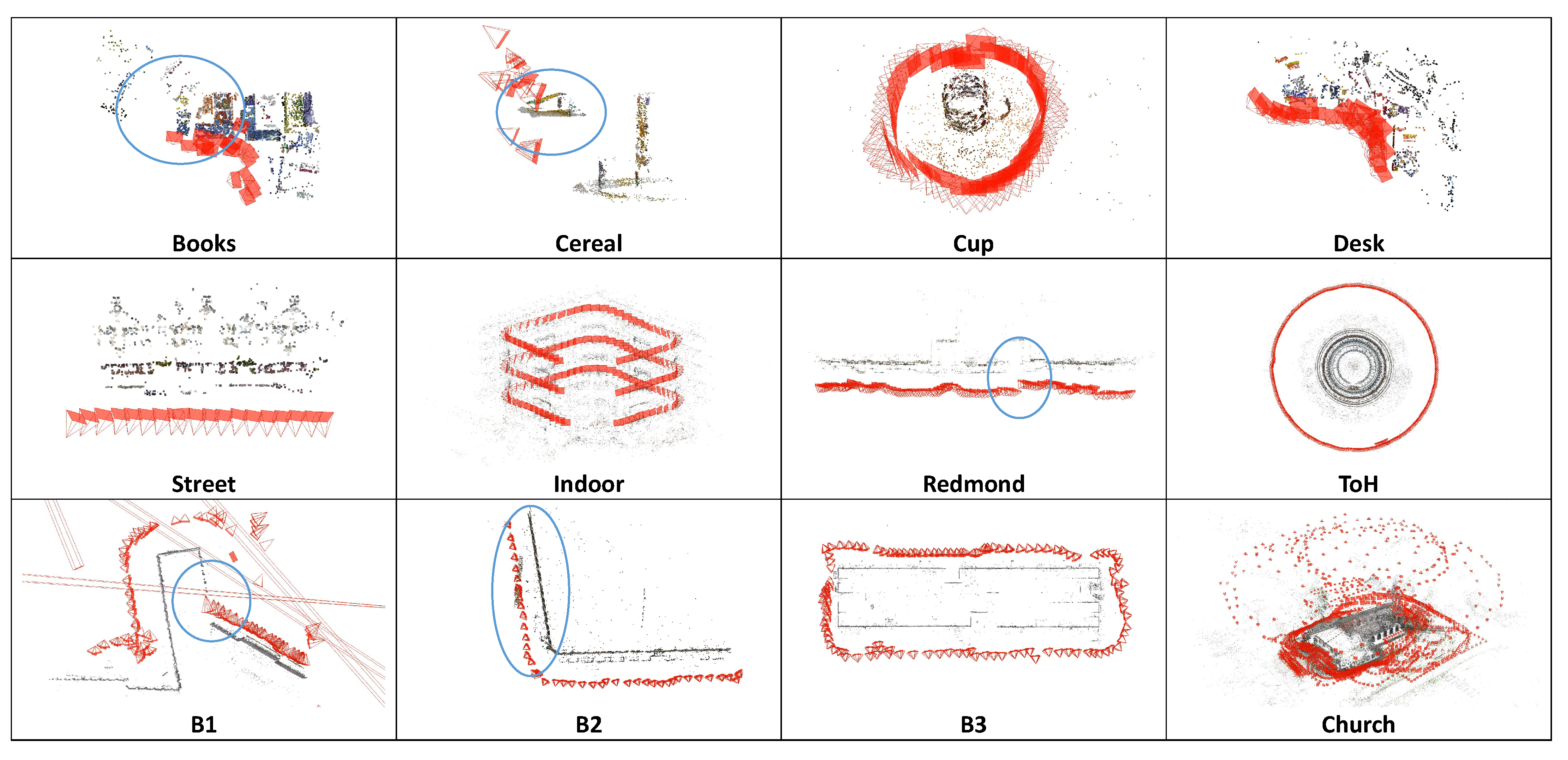
Church	1455	3264 × 2448 3648 × 2736 7360 × 4912	Repetitive structure Very short baselines	No

lists the image datasets used in our experiments, consisting of five small public datasets (Books, Cereal, Cup, Desk and Street [8]), three middle-scale datasets Indoor, Temple-of-Heaven (ToH) [8], and Redmond [41]), three benchmark datasets (B1, B2, B3 [26]), and one large image set (Church [29]). The “Type” column indicates two types of problematic match pairs: repetitive structure and very short baselines. To investigate the ability to cope with different problematic match pairs and demonstrate the performance of our method, eight image datasets with only repetitive structures were tested (Section 4.2 and Section 4.3), followed by three benchmark datasets with both repetitive structures and very short baselines (Section 4.4), and one large-scale dataset with repetitive structures and very short baselines (Section 4.5).

4.2. Performance on Five Small Datasets

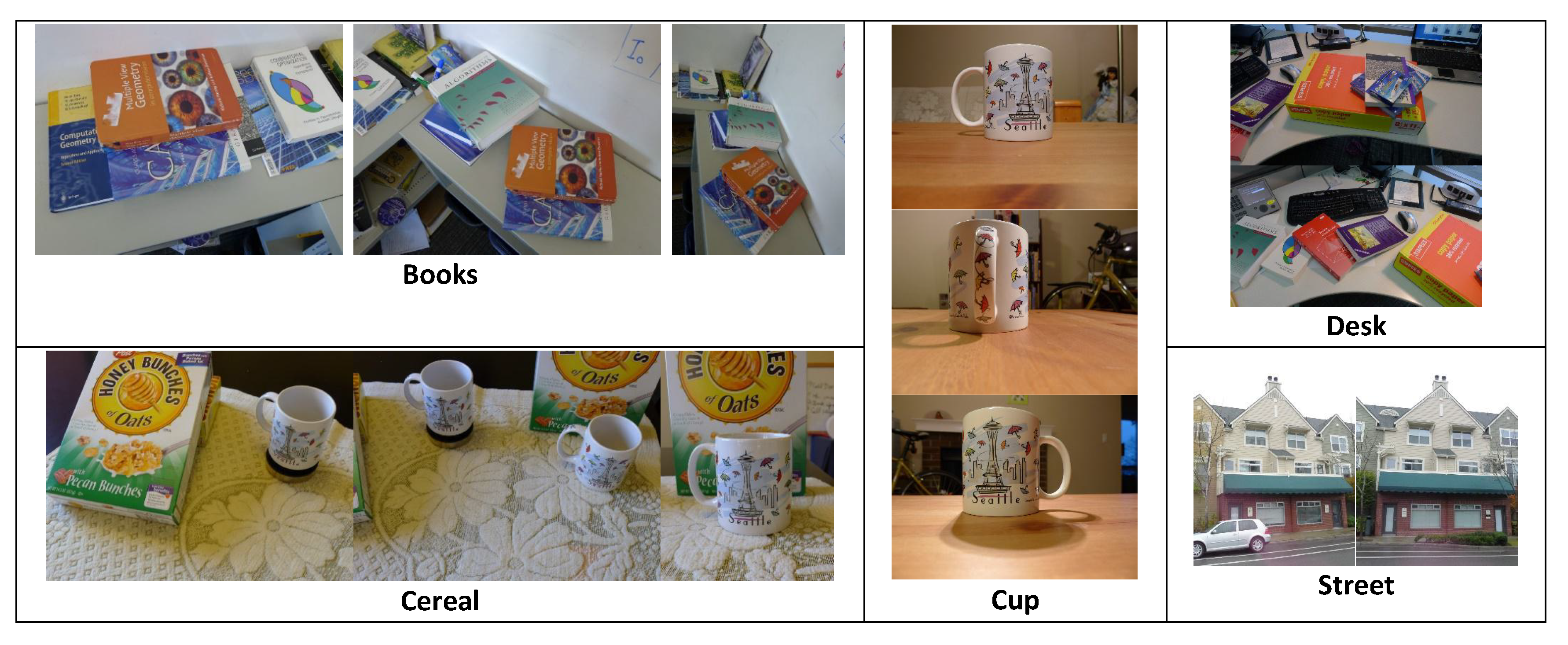
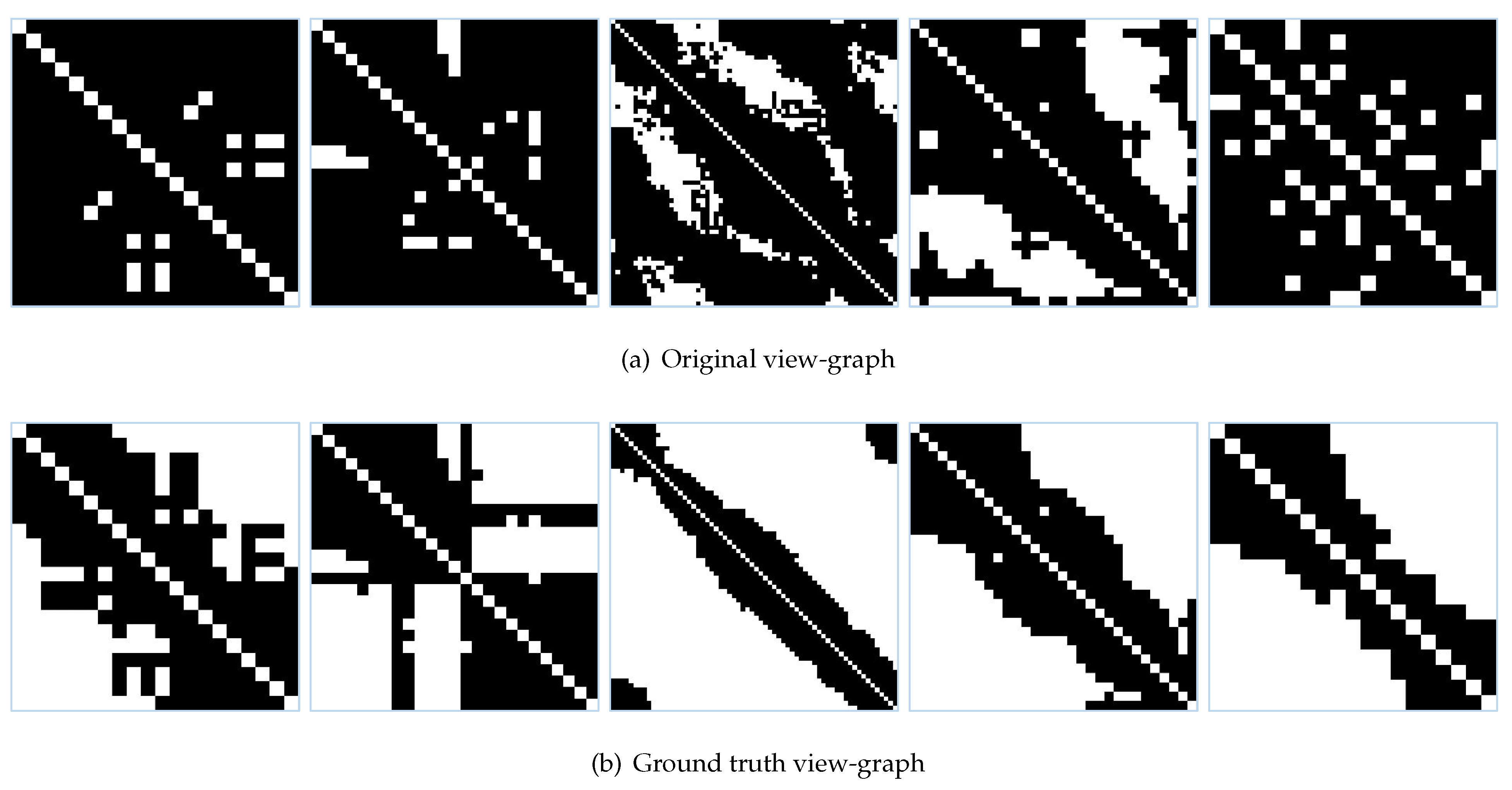
We tested five small datasets with different degrees of repetitive structures; some sample images are shown in Figure 9. Since these datasets were rather small, we could manually establish the ground-truth view-graph by selecting a subset with the correct overlapping relations of match pairs from the original view-graph. We used the adjacency matrix to represent the view-graph (see Figure 10), the horizontal and vertical directions of which indicate image IDs, and dark pixels indicate that the corresponding match pairs are considered correct. Figure 10a corresponds to the original view-graphs generated after the default matching process [10], and Figure 10b to the ground-truth view-graphs. We can see that the original view-graphs had many wrong match pairs stemming from the repetitive structure.

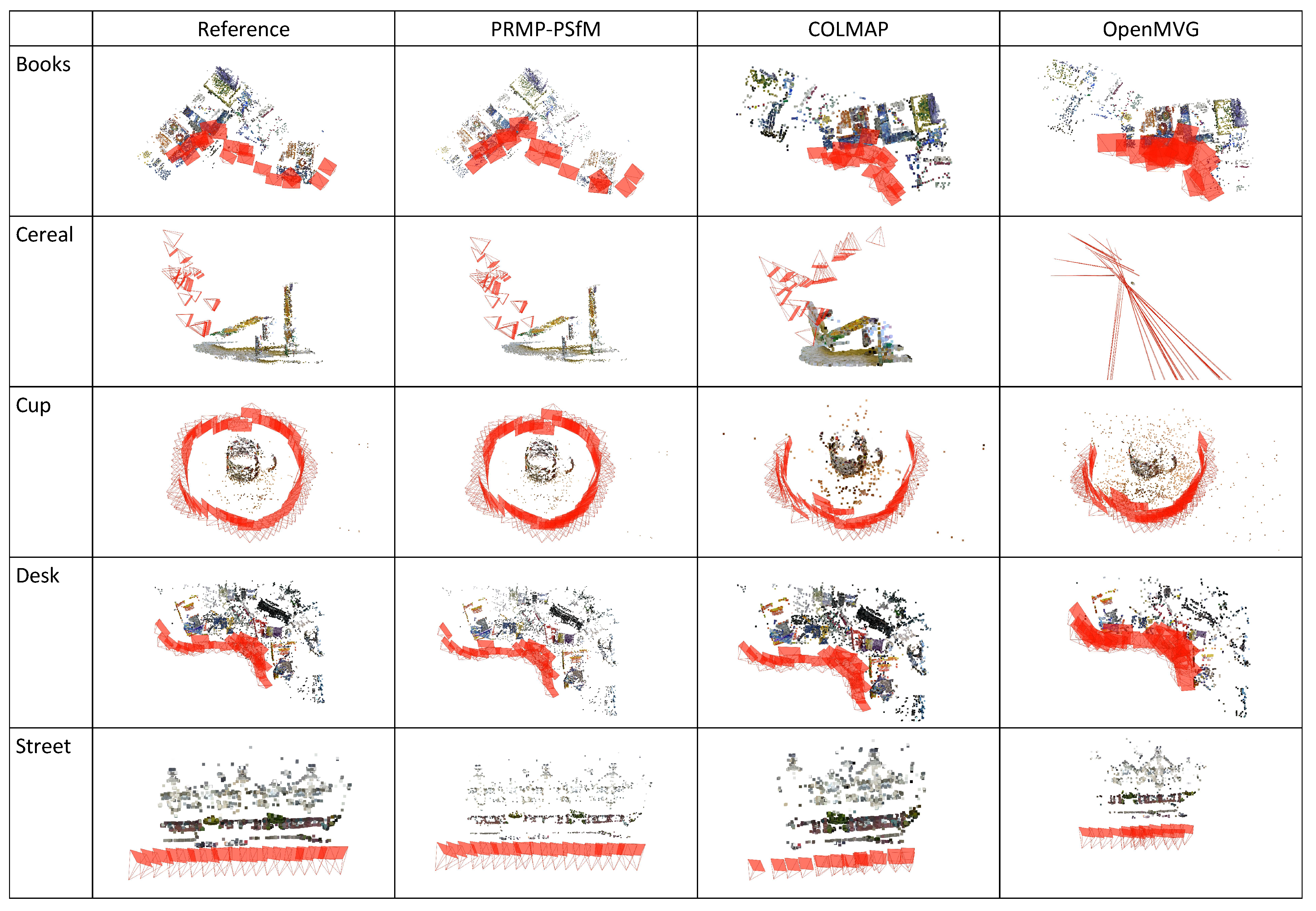
We inserted the ground-truth view-graphs (Figure 10b) in the incremental SfM pipeline (COLMAP, see Figure 1) to obtain reference reconstruction results, as shown in Figure 11. To compare different SfM methods, we input the original view-graphs (Figure 10a) to the PRMP-PSfM, COLMAP and OpenMVG SfM pipelines to determine whether they were capable of dealing with images of a repetitive structure. The reconstruction results from these five small datasets are shown in Figure 11. Compared to the reference, PRMP-PSfM generated the best reconstruction results for all five datasets; COLMAP and OpenMVG only successfully reconstructed the Desk dataset and obtained various folded structures for the other four datasets. For repetitive structures, wrong overlapping relations of image pairs in the original view-graph can possibly make the next-best view selection (Figure 1) invalid. We propose an improved method to overcome this by manipulating the view-graph, and PRMP-PSfM could generate the best SfM reconstruction results on all five datasets (with repetitive structures).

4.3. Performance on Three Middle-Scale Datasets with Repetitive Structures

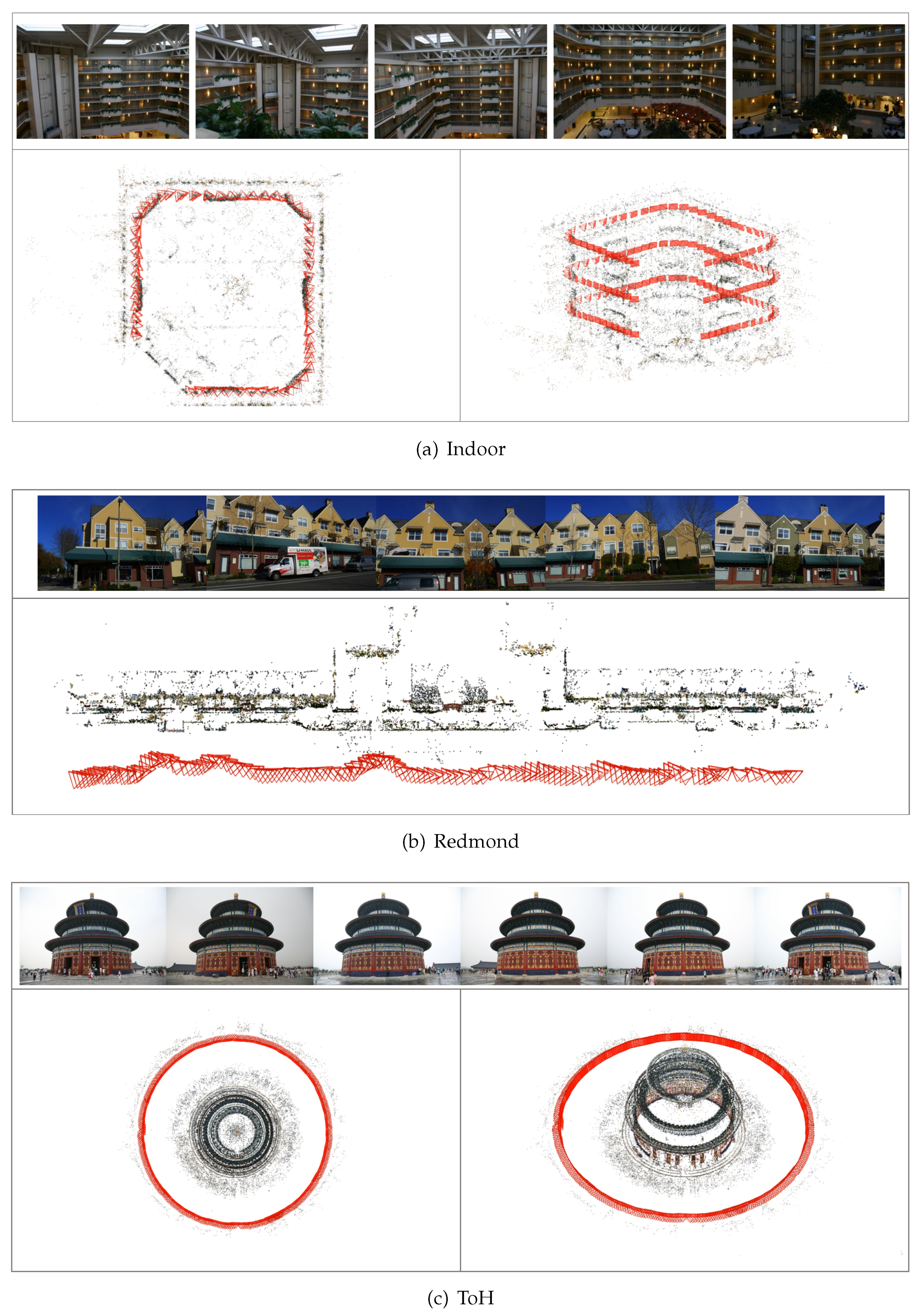
We reported on experiments on three middle-scale datasets with repetitive structures: Indoor, Redmond and ToH, whose sample images and reconstruction results are given in Figure 12a–c, respectively, [28]. The Indoor dataset was captured in an indoor scene, and its camera trajectory (red triangles) contained three single strips on three floors. For Redmond, the camera trajectory was nearly along a straight line when capturing a set of images in a row of some similar building facades. The scene of ToH contained nearly 360-degree symmetry, and images were captured with a closed loop.

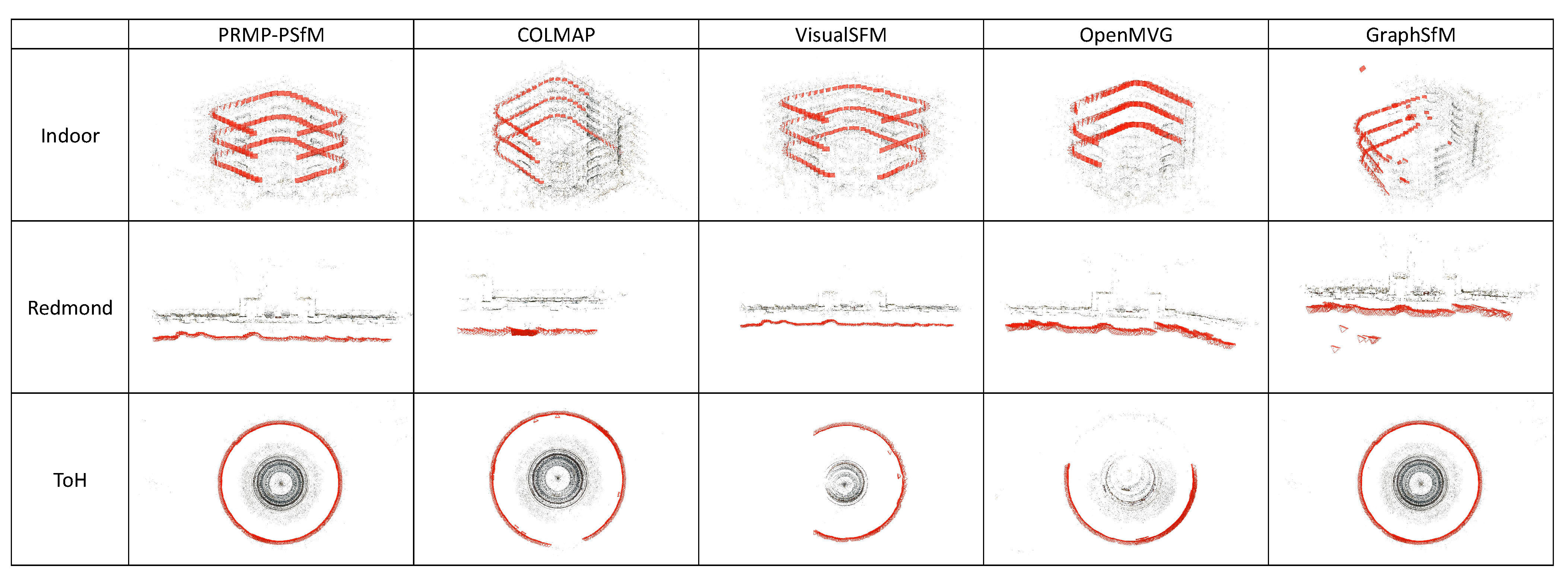
Because there are no ground-truths of these three datasets, based on visualization results [28] (see Figure 12), we carried out qualitative evaluations of PRMP-PSfM, COLMAP, VisualSFM, OpenMVG, and GraphSfM, whose reconstruction results are shown in Figure 13. For Indoor and Redmond, the results of PRMP-PSfM and VisualSFM were visually similar to the visualization results, but COLMAP, OpenMVG, and GraphSfM failed with regard to correct and complete the camera poses. For ToH, only PRMP-PSfM and GraphSfM were able to close the loop, while COLMAP, VisualSFM, and OpenMVG could only solve parts of the whole scene. We generated the best results on these three datasets, further demonstrating the capability of PRMP-PSfM to deal with images with repetitive structures.

4.4. Performance on Three Benchmark Datasets

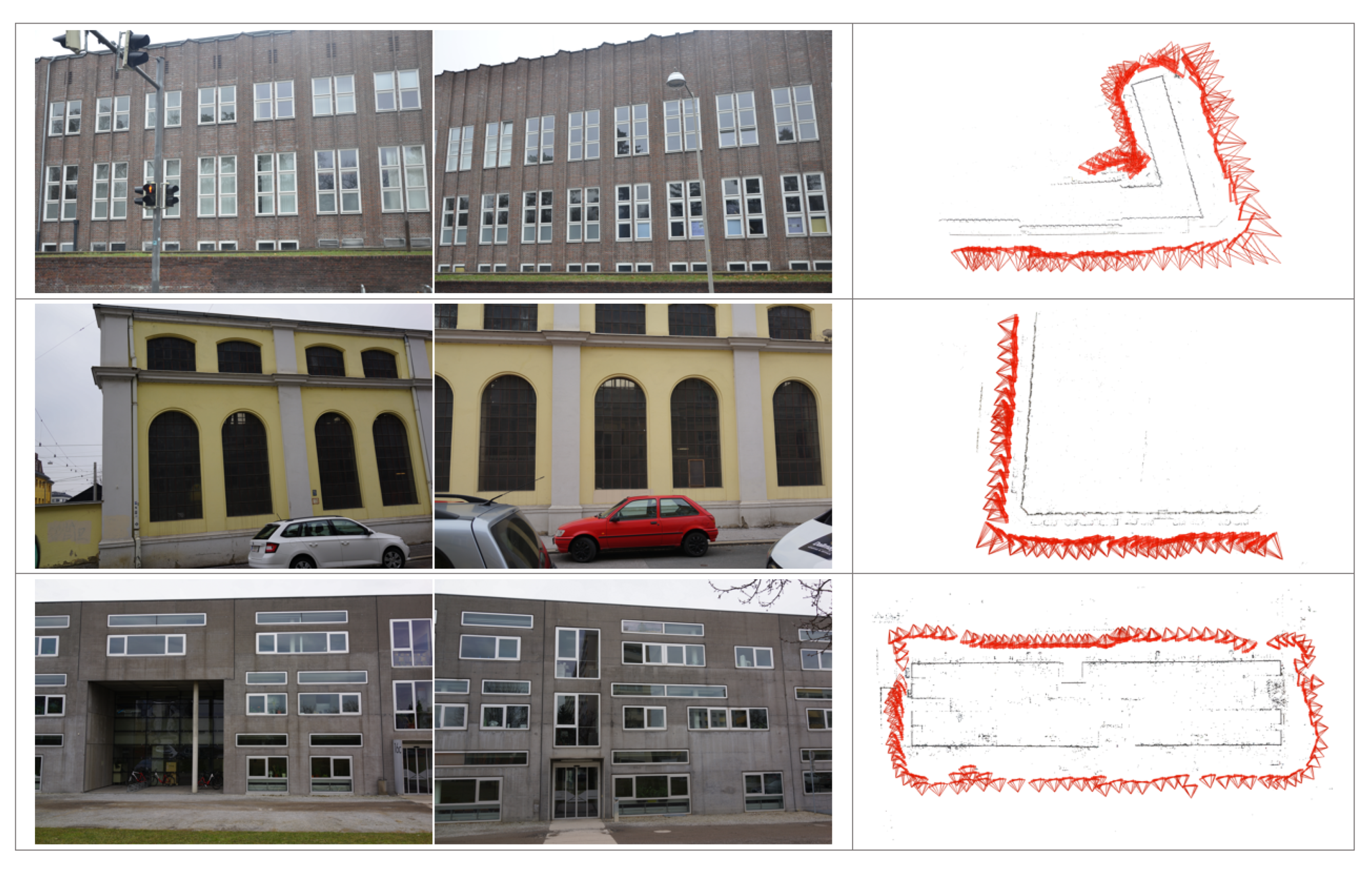
The ground-truth for benchmark datasets B1, B2 and B3 for match pairs [26] means that the corresponding correct match pairs and problematic ones due to repetitive structures and very short baselines were manually found and labeled. We inserted these correct match pairs in COLMAP to obtain reference reconstruction results, which, along with sample images, are shown in Figure 14.

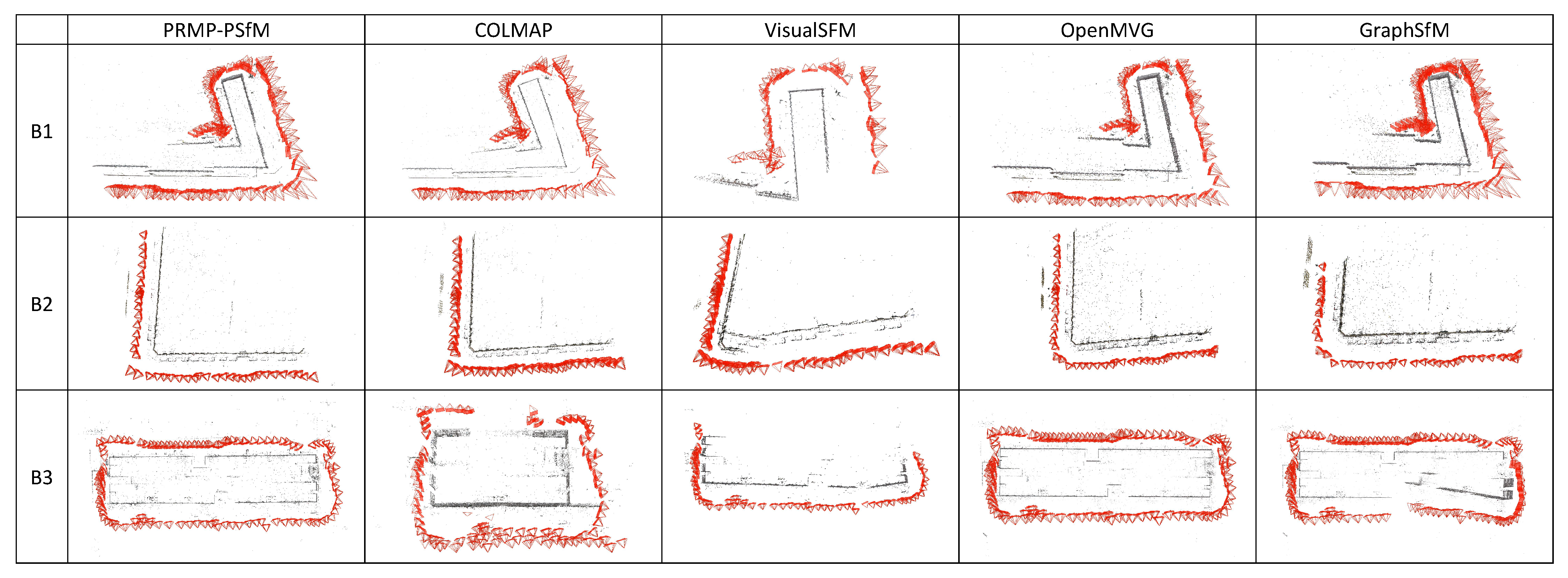
Figure 15 shows the final reconstruction results on these three benchmarks by the five SfM pipelines. Compared to the reference, only PRMP-PSfM and OpenMVG obtained similar results for all three datasets, while the other pipelines generated various visual drifts. For dataset B1, all pipelines except VisualSFM were able to obtain similar reconstruction results, which were generally identical to the reference. PRMP-PSfM, COLMAP, and OpenMVG were able to reconstruct dataset B2, but the result of VisualSFM showed large drift, and GraphSfM only recovered part of the scene. Dataset B3 contained a closed loop around one building, and only PRMP-PSfM and OpenMVG could recover a complete reconstruction. To further demonstrate the performance of PRMP-PSfM, we quantitatively evaluated the reconstruction results that were qualitatively similar to the reference, i.e., those of B1 and B2 by PRMP-PSfM, COLMAP and OpenMVG, and those of B3 by PRMP-PSfM and OpenMVG. We calculated the rotation and translation errors, which are listed in

Table 3. Quantitative evaluation for benchmark datasets B1, B2 and B3. Rotation error is the angular difference from the reference, in degrees; translation error is the position difference from the reference in ground-truth units.

Dataset	Pipeline	Rotation Error				Translation Error ($\times {10}^{-2}$)
		$\mathit{Min}$	$\mathit{Mean}$	$\mathit{Median}$	$\mathit{Max}$	$\mathit{Min}$	$\mathit{Mean}$	$\mathit{Median}$	$\mathit{Max}$
B1	PRMP-PSfM	0.02	0.11	0.13	0.52	0.11	0.53	0.54	3.21
	COLMAP	0.17	1.47	1.27	2.21	1.25	8.93	9.78	18.4
	OpenMVG	0.18	1.7	1.63	3.74	1.55	10.02	10.40	18.66
B2	PRMP-PSfM	0.03	0.08	0.07	0.32	0.08	0.55	0.49	3.27
	COLMAP	0.15	0.91	1.02	1.84	1.05	4.58	4.86	9.89
	OpenMVG	0.15	0.66	0.46	4.54	0.22	7.29	4.84	48.61
B3	PRMP-PSfM	0.02	0.10	0.09	0.46	0.06	0.74	0.66	2.89
	OpenMVG	0.06	0.39	0.40	0.89	0.58	3.02	2.55	88.61

. It can be seen that our method obtained the highest accuracy on all three datasets. Although PRMP-PSfM and OpenMVG were able to obtain visually similar results, the numerical evaluation in Table 3 shows that reconstruction results of OpenMVG were less accurate than those of PRMP-PSfM. In particular, the results of max rotation error and max translation error indicate that some of the camera poses of OpenMVG were gross errors. In contrast, PRMP-PSfM was able to estimate the accurate rotation and translation parameters for all images, which shows its superiority at coping with problematic match pairs.

4.5. Performance on a Large-Scale Dataset

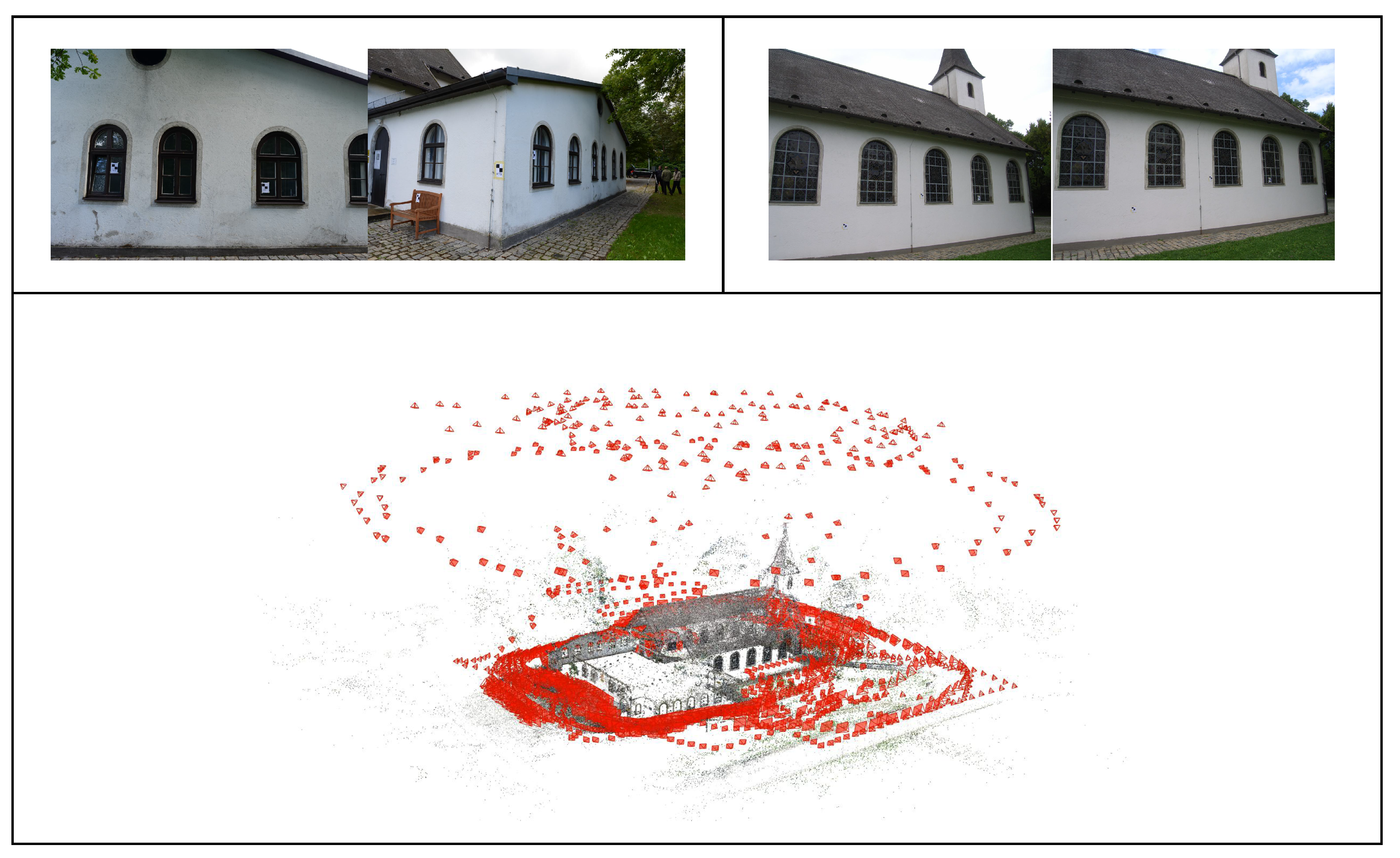
We evaluated PRMP-PSfM on the large-scale Church dataset [29], which consisted of 1455 unordered images with repetitive structures and very short baselines. Sample match pairs and our reconstruction results are shown in Figure 16. We present the numerical evaluation of five incremental and one hierarchical SfM pipeline in

Table 4. Numerical comparison on Church dataset for different SfM pipelines. $N_{img}$ is the number of orientated images in the final reconstruction results, and the % values refer to the number of orientated images compared with that of the input images, ${\delta }_0$ is the mean projection error in pixels, $N_p$ is the number of tie points, and “-” indicates that the corresponding items are unavailable.

Pipeline	${\mathit{N}}_{\mathit{img}}(\%)$	${\mathit{\delta }}_0$	${\mathit{N}}_{\mathit{p}}$
PRMP-PSfM	1448 (99.5)	0.37	491,992
COLMAP	1454 (99.9)	1.09	549,957
VisualSFM	288(19.8)	0.74	14,295
OpenMVG	1452 (99.8)	0.54	1,687,694
GraphSfM	1439 (98.9)	0.51	2,762,371
APE	-	0.55	290,748

. The results of COLMAP, OpenMVG, and GraphSfM were obtained with default settings, and those of APE and VisualSFM are cited from Michelini et al. [29]. In terms of completeness, all pipelines except VisualSFM were able to orientate more than 98.9% of images, while COLMAP gave the most complete result (up to 99.9% of all images were solved). PRMP-PSfM, OpenMVG, GraphSfM, and APE generated similar mean reprojection errors, while COLMAP obtained the largest, implying that COLMAP did not obtain a convergent result. There are various reasons for the big differences in the number of reconstructed 3D points of these pipelines, such as different settings for feature extraction and rules for selecting tracks. PRMP-PSfM and COLMAP deleted tracks only observed by two images, while OpenMVG and GraphSfM retained them. Hence, it can be concluded that PRMP-PSfM, OpenMVG, GraphSfM, and APE obtained comparable precision and completeness results.

4.6. Performance of without Iteratively Refining Match Pairs

In PRMP-PSfM, the process of iteratively refining match pairs is implemented by repeatedly executing “outlier elimination using CCI” (Figure 5). To investigate how it influences SfM reconstruction results, we turned off that function. Figure 17 shows the reconstruction results for all datasets by PRMP-PSfM without iteratively refining match pairs, which we refer to as PSfM. Blue ellipses indicate visual drifts. The generated drifts in Books and Redmond were due to ambiguous tracks generated from match pairs with repetitive structures. The results of Cereal and B1 contained large-scale drifts (see blue ellipses), which occurred at the beginning of the expansion. The reconstruction result of B2 was negatively influenced by a repetitive structure and very short baselines.

We show a numerical comparison for the four datasets whose reconstruction results of PRMP-PSfM and PSfM were visually similar, i.e., Cup, Desk, Street and B3, in

Table 5. Numerical comparison of reconstruction results between PRMP-PSfM and PSfM. ${\delta }_0$ is the mean projection error, $m_r$ is the mean rotation error in degrees and $m_t$ is the mean translation error in ground-truth units $\times {10}^{-1}$.

Dataset	PRMP-PSfM			PSfM
	${\mathit{\delta }}_0$	${\mathit{m}}_{\mathit{r}}$	${\mathit{m}}_{\mathit{t}}$	${\mathit{\delta }}_0$	${\mathit{m}}_{\mathit{r}}$	${\mathit{m}}_{\mathit{t}}$
Cup	0.26	0.67	0.23	0.26	0.73	0.23
Desk	0.32	1.32	0.90	0.47	6.46	1.78
Street	0.18	0.78	0.11	0.35	1.16	0.29
B3	0.39	0.06	0.16	0.36	0.35	0.42

. Regarding the reprojection error, PRMP-PSfM showed better performance on Desk and Street and comparable results on Cup and B3. For errors on camera poses, we calculated the discrepancies between their results and the reference ones. PRMP-PSfM obtained higher accuracy than PSfM on both rotation and translation.

4.7. Settings of Parameter $\alpha$

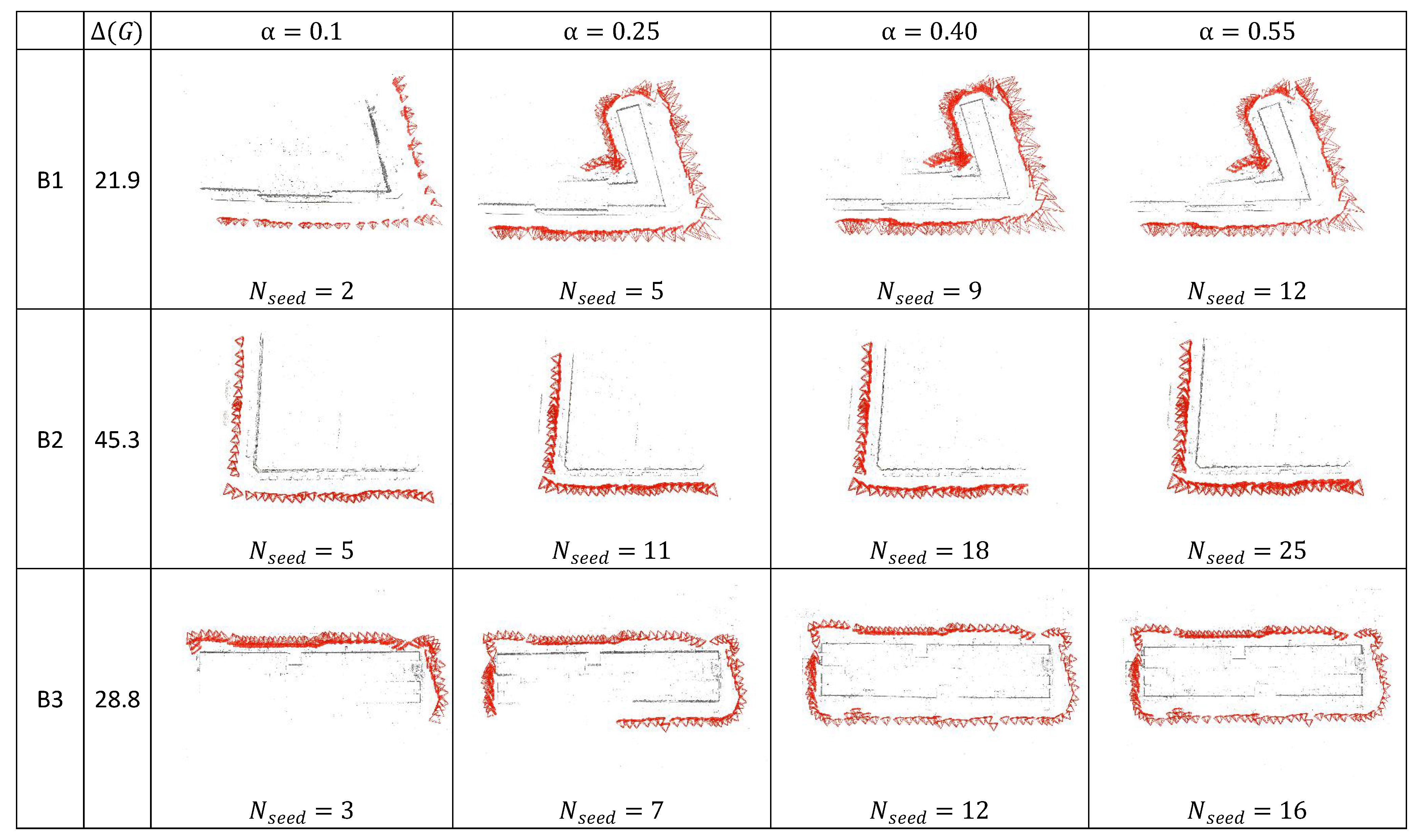
To investigate to what degree the key parameter $\alpha$ can influence the performance of PRMP-PSfM, we alternated the value of the free parameter $\alpha$ to qualitatively and quantitatively evaluate it on benchmark datasets B1, B2 and B3, with results as shown in Figure 18 and

Table 6. Numerical comparisons of seed reconstruction results from different values of $\alpha$. $N_{img}$ is the number of orientated images in the final reconstruction results. $m_r$ is the mean rotation error in degrees and $m_t$ is the mean translation error in ground-truth units $\times {10}^{-2}$.

Dataset	$\mathit{\alpha }=0.1$			$\mathit{\alpha }=0.25$			$\mathit{\alpha }=0.40$			$\mathit{\alpha }=0.55$
	${\mathit{N}}_{\mathit{img}}$	${\mathit{m}}_{\mathit{r}}$	${\mathit{m}}_{\mathit{t}}$	${\mathit{N}}_{\mathit{img}}$	${\mathit{m}}_{\mathit{r}}$	${\mathit{m}}_{\mathit{t}}$	${\mathit{N}}_{\mathit{img}}$	${\mathit{m}}_{\mathit{r}}$	${\mathit{m}}_{\mathit{t}}$	${\mathit{N}}_{\mathit{img}}$	${\mathit{m}}_{\mathit{r}}$	${\mathit{m}}_{\mathit{t}}$
B1	109	0.93	7.82	182	0.11	0.53	182	0.18	1.24	182	1.47	8.89
B2	215	0.06	0.51	215	0.08	0.55	215	0.31	1.08	215	0.43	1.22
B3	182	0.26	1.26	275	0.22	1.07	342	0.35	1.44	342	0.47	1.93

. Figure 18 shows the seed reconstruction results (Section 3.4) obtained for different values of $\alpha$. Table 6 shows the discrepancies between these and the reference results. As emphasized in Section 3.4, the objective of initialization is to obtain good seed reconstruction. As Table 6 shows, when setting $\alpha =0.25$, our initialization step obtained the highest accuracy on B1 and B3, and accuracy on B2 comparable to that of $\alpha =0.1$. We obtained the best result on B2 with $\alpha =0.1$, but less accurate results on B1 and B3. Accuracy was lower for $\alpha =0.40$ and $\alpha =0.55$, because a denser view-graph leads to a higher possibility of including incorrect match pairs.

The case of $\alpha =0.25$ was good enough for complete reconstruction results on B1 and B2, revealing that PRMP-PSfM achieved the final reconstruction results by only applying the seed view-graph. Compared with other pipelines at handling the full view-graph, PRMP-PSfM has good potential to improve efficiency.

5. Discussion

We investigate some characteristics of PRMP-PSfM and discuss the effect of iteratively prioritizing match pairs (Section 5.2) and the effect of iteratively refining match pairs (Section 5.1). A limitation on the condition of completeness is discussed in Section 5.3.

5.1. Effect of Iteratively Refining Match Pairs

In Section 4.6, without iteratively refining match pairs, our PRMP-PSfM becomes PSfM. From the visualization results in Figure 17, it can be seen that PSfM produced worse results than PRMP-PSfM, which could successfully reconstruct all these datasets (Figure 11, Figure 13, Figure 15 and Figure 16). According to the numerical comparison presented in Table 5, PSfM obtained lower accuracy on SfM reconstruction. These results indicate that without iteratively refining match pairs, the outliers in match pairs degraded the SfM reconstruction results of PRMP-PSfM. In other words, iteratively refining match pairs can benefit PRMP-PSfM in regard to robustness and accuracy.

5.2. Effect of Iteratively Prioritizing Match Pairs

Iteratively prioritizing match pairs using MST yields the progressive scheme on view-graph, which aims to generate the filtered seed view-graph, and subsequently expands until the complete reconstruction is achieved. COLMAP directly applies the original view-graph, whereas PSfM employs the progressive scheme on the view-graph. Comparing the results of COLMAP (Figure 11, Figure 13, Figure 15 and Figure 16) and PSfM (Figure 17), we can see that for datasets with a repetitive structure only, PSfM could successfully handle Cup, Desk, Street, Indoor, and ToH. In contrast, COLMAP could only obtain good results for Desk. This shows the advantages of the progressive scheme at handling images with repetitive structures. However, PSfM failed on Books, Cereal, and Redmond because the prioritized match pairs still exist some outliers that need to be eliminated. This demonstrates that only using the progressive scheme cannot perfectly prevent the negative influence of outliers in match pairs and implies that refining match pairs is necessary.

5.3. Limitation on Condition of Completeness

We discuss one limitation on the condition of completeness. For Church (Table 4), the condition of completeness that all images are successfully orientated could not be strictly met. For this dataset, the original view-graph obtained in PRMP-PSfM contained 1454 images, which was actually not 100% of all images. In the expansion period, some images causing the refinement of bundle adjustment to not converge were filtered. Hence, we set a relaxed condition of completeness, that 95% of images contained in the original view-graph were solved. Thus, the setting on the condition of completeness might need to be adjusted when dealing with various image sets, e.g., those containing both terrestrial and UAV images.

6. Conclusions

The SfM pipeline PRMP-PSfM was proposed for robust and accurate reconstruction from images with problematic match pairs due to repetitive structures and very short baselines; it can also be considered an improved incremental method. The limitations of conventional incremental methods in dealing with these problematic match pairs were discussed. All potential match pairs were first cast into a weighted view-graph, which could be manipulated to form a progressive scheme with initialization and expansion. In the initialization step, a subset of match pairs was prioritized using multiple MSTs. This was refined using an outlier elimination technique of consistency inference or CCI to generate the filtered seed view-graph for good seed reconstruction, which was expanded for more complete reconstruction by progressively adding new MSTs. As the reconstruction expanded, new match pairs were iteratively refined before carrying out the SfM process at each iteration. The above steps compose PRMP-PSfM, whose performance was demonstrated on datasets with repetitive structures and very short baselines. Experimental results showed that PRMP-PSfM could achieve better robustness and accuracy on reconstruction results than several state-of-the-art incremental and hierarchical SfM methods. Some cases may require the relaxation of the condition of completeness used in PRMP-PSfM. In the future, we hope to improve the condition of completeness and combine PRMR-PSfM with hierarchical SfM to efficiently deal with large-scale image sets.

References

- Förstner, W.; Wrobel, B.P. Photogrammetric Computer Vision; Springer: Berlin/Heidelberg, Germany, 2016. [Google Scholar]
- McGlone, C.; Mikhail, E.; Bethel, J. Manual of Photogrammetry, 5th ed.; American Society of Photogrammetry: Falls Church, VA, USA, 2004. [Google Scholar]
- Lowe, D.G. Distinctive image features from scale-invariant keypoints. Int. J. Comput. Vis. 2004, 60, 91–110. [Google Scholar] [CrossRef]
- Longuet-Higgins, H.C. A computer algorithm for reconstructing a scene from two projections. Nature 1981, 293, 133–135. [Google Scholar] [CrossRef]
- Stewenius, H.; Engels, C.; Nistér, D. Recent developments on direct relative orientation. ISPRS J. Photogramm. Remote Sens. 2006, 60, 284–294. [Google Scholar] [CrossRef]
- Fischler, M.A.; Bolles, R.C. Random sample consensus: A paradigm for model fitting with applications to image analysis and automated cartography. Commun. ACM 1981, 24, 381–395. [Google Scholar] [CrossRef]
- Sweeney, C.; Sattler, T.; Hollerer, T.; Turk, M.; Pollefeys, M. Optimizing the viewing graph for structure-from-motion. In Proceedings of the IEEE International Conference on Computer Vision, Santiago, Chile, 7–13 December 2015; pp. 801–809. [Google Scholar]
- Shen, T.; Zhu, S.; Fang, T.; Zhang, R.; Quan, L. Graph-based consistent matching for structure-from-motion. In European Conference on Computer Vision; Springer: Berlin/Heidelberg, Germany, 2016; pp. 139–155. [Google Scholar]
- Cui, H.; Shi, T.; Zhang, J.; Xu, P.; Meng, Y.; Shen, S. View-graph construction framework for robust and efficient structure-from-motion. Pattern Recognit. 2020, 114, 107712. [Google Scholar] [CrossRef]
- Schonberger, J.L.; Frahm, J.M. Structure-from-motion revisited. In Proceedings of the IEEE Conference on Computer Vision and Pattern Recognition, Las Vegas, NV, USA, 27–30 June 2016; pp. 4104–4113. [Google Scholar]
- Wang, X.; Xiao, T.; Kasten, Y. A hybrid global structure from motion method for synchronously estimating global rotations and global translations. ISPRS J. Photogramm. Remote Sens. 2021, 174, 35–55. [Google Scholar] [CrossRef]
- Snavely, N.; Seitz, S.M.; Szeliski, R. Modeling the World from Internet Photo Collections. Int. J. Comput. Vis. 2008, 80, 189–210. [Google Scholar] [CrossRef] [Green Version]
- Hartley, R.; Zisserman, A. Multiple View Geometry in Computer Vision; Cambridge University Press: Cambridge, UK, 2003. [Google Scholar]
- Triggs, B.; McLauchlan, P.F.; Hartley, R.I.; Fitzgibbon, A.W. Bundle adjustment—A modern synthesis. In International Workshop on Vision Algorithms; Springer: Berlin/Heidelberg, Germany, 1999; pp. 298–372. [Google Scholar]
- Wu, C. Towards linear-time incremental structure from motion. In Proceedings of the 2013 International Conference on 3D Vision-3DV 2013, Seattle, WA, USA, 29 June–1 July 2013; IEEE: Piscataway, NJ, USA, 2013; pp. 127–134. [Google Scholar]
- Mayer, H. Efficient hierarchical triplet merging for camera pose estimation. In German Conference on Pattern Recognition; Springer: Berlin/Heidelberg, Germany, 2014; pp. 399–409. [Google Scholar]
- Toldo, R.; Gherardi, R.; Farenzena, M.; Fusiello, A. Hierarchical structure-and-motion recovery from uncalibrated images. Comput. Vis. Image Underst. 2015, 140, 127–143. [Google Scholar] [CrossRef] [Green Version]
- Xie, X.; Yang, T.; Li, D.; Li, Z.; Zhang, Y. Hierarchical clustering-aligning framework based fast large-scale 3D reconstruction using aerial imagery. Remote Sens. 2019, 11, 315. [Google Scholar] [CrossRef] [Green Version]
- Chen, Y.; Shen, S.; Chen, Y.; Wang, G. Graph-based parallel large scale structure from motion. Pattern Recognit. 2020, 107, 107537. [Google Scholar] [CrossRef]
- Govindu, V.M. Robustness in motion averaging. In Asian Conference on Computer Vision; Springer: Berlin/Heidelberg, Germany, 2006; pp. 457–466. [Google Scholar]
- Wilson, K.; Snavely, N. Robust global translations with 1dsfm. In European Conference on Computer Vision; Springer: Berlin/Heidelberg, Germany, 2014; pp. 61–75. [Google Scholar]
- Agarwal, S.; Furukawa, Y.; Snavely, N.; Simon, I.; Curless, B.; Seitz, S.M.; Szeliski, R. Building rome in a day. Commun. ACM 2011, 54, 105–112. [Google Scholar] [CrossRef]
- Wang, X.; Rottensteiner, F.; Heipke, C. Structure from motion for ordered and unordered image sets based on random kd forests and global pose estimation. ISPRS J. Photogramm. Remote Sens. 2019, 147, 19–41. [Google Scholar] [CrossRef]
- Jiang, S.; Jiang, C.; Jiang, W. Efficient structure from motion for large-scale UAV images: A review and a comparison of SfM tools. ISPRS J. Photogramm. Remote Sens. 2020, 167, 230–251. [Google Scholar] [CrossRef]
- Cui, H.; Shen, S.; Gao, W.; Liu, H.; Wang, Z. Efficient and robust large-scale structure-from-motion via track selection and camera prioritization. ISPRS J. Photogramm. Remote Sens. 2019, 156, 202–214. [Google Scholar] [CrossRef]
- Wang, X.; Xiao, T.; Gruber, M.; Heipke, C. Robustifying relative orientations with respect to repetitive structures and very short baselines for global SfM. In Proceedings of the IEEE Conference on Computer Vision and Pattern Recognition Workshops, Long Beach, CA, USA, 16–17 June 2019. [Google Scholar]
- Enqvist, O.; Kahl, F.; Olsson, C. Non-sequential structure from motion. In Proceedings of the 2011 IEEE International Conference on Computer Vision Workshops (ICCV Workshops), Barcelona, Spain, 6–13 November 2011; IEEE: Piscataway, NJ, USA, 2011; pp. 264–271. [Google Scholar]
- Wang, X.; Heipke, C. An Improved Method of Refining Relative Orientation in Global Structure from Motion with a Focus on Repetitive Structure and Very Short Baselines. Photogramm. Eng. Remote Sens. 2020, 86, 299–315. [Google Scholar] [CrossRef]
- Michelini, M.; Mayer, H. Structure from motion for complex image sets. ISPRS J. Photogramm. Remote Sens. 2020, 166, 140–152. [Google Scholar] [CrossRef]
- Jiang, N.; Tan, P.; Cheong, L.F. Seeing double without confusion: Structure-from-motion in highly ambiguous scenes. In Proceedings of the 2012 IEEE Conference on Computer Vision and Pattern Recognition, Providence, RI, USA, 16–21 June 2012; IEEE: Piscataway, NJ, USA, 2012; pp. 1458–1465. [Google Scholar]
- Heinly, J.; Dunn, E.; Frahm, J.M. Correcting for duplicate scene structure in sparse 3D reconstruction. In European Conference on Computer Vision; Springer: Berlin/Heidelberg, Germany, 2014; pp. 780–795. [Google Scholar]
- Zach, C.; Klopschitz, M.; Pollefeys, M. Disambiguating visual relations using loop constraints. In Proceedings of the 2010 IEEE Computer Society Conference on Computer Vision and Pattern Recognition, San Francisco, CA, USA, 13–18 June 2010; IEEE: Piscataway, NJ, USA, 2010; pp. 1426–1433. [Google Scholar]
- Moulon, P.; Monasse, P.; Perrot, R.; Marlet, R. Openmvg: Open multiple view geometry. In International Workshop on Reproducible Research in Pattern Recognition; Springer: Berlin/Heidelberg, Germany, 2016; pp. 60–74. [Google Scholar]
- Jiang, N.; Cui, Z.; Tan, P. A global linear method for camera pose registration. In Proceedings of the IEEE International Conference on Computer Vision, Sydney, Australia, 1–8 December 2013; pp. 481–488. [Google Scholar]
- Cui, H.; Shen, S.; Gao, W.; Wang, Z. Progressive large-scale structure-from-motion with orthogonal msts. In Proceedings of the 2018 International Conference on 3D Vision (3DV), Verona, Italy, 5–8 September 2018; IEEE: Piscataway, NJ, USA, 2018; pp. 79–88. [Google Scholar]
- Snavely, N.; Seitz, S.M.; Szeliski, R. Skeletal graphs for efficient structure from motion. In Proceedings of the 2008 IEEE Conference on Computer Vision and Pattern Recognition, Anchorage, AK, USA, 24–26 June 2008; IEEE: Piscataway, NJ, USA, 2008; pp. 1–8. [Google Scholar]
- Cui, Z.; Jiang, N.; Tang, C.; Tan, P. Linear Global Translation Estimation with Feature Tracks. Proc. ECCV 2014, 3, 61–75. [Google Scholar]
- Kschischang, F.R.; Frey, B.J.; Loeliger, H.A. Factor graphs and the sum-product algorithm. IEEE Trans. Inf. Theory 2001, 47, 498–519. [Google Scholar] [CrossRef] [Green Version]
- Prim, R.C. Shortest Connection Networks and Some Generalizations. Bell Syst. Tech. J. 1957, 36, 1389–1401. [Google Scholar] [CrossRef]
- Cheng, J.; Leng, C.; Wu, J.; Cui, H.; Lu, H. Fast and accurate image matching with cascade hashing for 3D reconstruction. In Proceedings of the IEEE Conference on Computer Vision and Pattern Recognition, Columbus, OH, USA, 23–28 June 2014; pp. 1–8. [Google Scholar]
- Cohen, A.; Zach, C.; Sinha, S.N.; Pollefeys, M. Discovering and exploiting 3D symmetries in structure from motion. In Proceedings of the 2012 IEEE Conference on Computer Vision and Pattern Recognition, Providence, RI, USA, 16–21 June 2012; IEEE: Piscataway, NJ, USA, 2012; pp. 1514–1521. [Google Scholar]
Figure 1.
Workflow of COLMAP [10].
Figure 2.
Example of a repetitive structure: (a) a correct match pair, and (b) a wrong match pair due to repetitive structure, where colored lines show correspondences; (c) original view-graph estimated by COLMAP; (d) reconstruction result from inputting (c) in [10], where red triangles describe camera poses; (e) filtered view-graph, and (f) corresponding reconstruction result, where edges in (e) are correct match pairs manually selected from (c).
Figure 3.
Different cases of two-view intersection with a constant baseline. Blue, red and black points indicate two images and one 3D point, respectively. Blue and red arrows indicate two view rays. The radius of circle (dotted line) indicates a constant baseline between two images.
Figure 4.
Example of very short baselines: (a) the reference reconstruction result; (b) initial two-view reconstruction; (c–f) reconstruction results as the block grows, where blue ellipses indicate areas where 3D points are incorrectly estimated.
Figure 5.
Workflow of PRMP-PSfM.
Figure 6.
Illustrative process of outlier elimination using CCI to filter incorrect match pairs: (a) input original view-graph, where red vertices indicate images and gray edges are match pairs; (b) procedure of cycle extraction on view-graph, where only some sample cycles are highlighted by blue lines; (c) CCI infers incorrect edges, which are highlighted by black lines; and (d) filtered view-graph after eliminating incorrect edges.
Figure 7.
Illustrative process of generating the filtered seed view-graph: (a) original view-graph; (b) seed view-graphs obtained by uniting a number of MSTs; and (c) filtered seed view-graph after outlier elimination using CCI.
Figure 8.
Workflow of expansion of seed reconstruction.
Figure 9.
Sample images of five small datasets with repetitive structures.
Figure 10.
Adjacency matrices of view-graph for five small datasets. From left to right: Books, Cereal, Cup, Desk, Street.
Figure 11.
Reconstruction results from five small datasets.
Figure 12.
Sample images and reconstruction results [28] of three middle-scale datasets with repetitive structures.
Figure 13.
Reconstruction results on three middle-scale datasets with repetitive structures.
Figure 14.
Sample images and correct reconstruction results of three benchmark datasets with both repetitive structures and very short baselines. From top to bottom: B1, B2 and B3.
Figure 15.
Reconstruction results of three benchmark datasets from different SfM pipelines.
Figure 16.
Sample images and our reconstruction result of the Church dataset. The top shows the sample match pairs, and on the left and right are match pairs due to repetitive structure and very short baselines, respectively. The bottom shows our SfM reconstruction result.
Figure 17.
Reconstruction results for various datasets by PSfM, i.e., PRMP-PSfM without iteratively refining match pairs.
Figure 18.
Seed reconstruction results for different values of .