Inter-Comparison of Methods for Chlorophyll-a Retrieval: Sentinel-2 Time-Series Analysis in Italian Lakes

Abstract

Different methods are available for retrieving chlorophyll-a (Chl-a) in inland waters from optical imagery, but there is still a need for an inter-comparison among the products. Such analysis can provide insights into the method selection, integration of products, and algorithm development. This work aims at inter-comparison and consistency analyses among the Chl-a products derived from publicly available methods consisting of Case-2 Regional/Coast Colour (C2RCC), Water Color Simulator (WASI), and OC3 (3-band Ocean Color algorithm). C2RCC and WASI are physics-based processors enabling the retrieval of not only Chl-a but also total suspended matter (TSM) and colored dissolved organic matter (CDOM), whereas OC3 is a broadly used semi-empirical approach for Chl-a estimation. To pursue the inter-comparison analysis, we demonstrate the application of Sentinel-2 imagery in the context of multitemporal retrieval of constituents in some Italian lakes. The analysis is performed for different bio-optical conditions including subalpine lakes in Northern Italy (Garda, Idro, and Ledro) and a turbid lake in Central Italy (Lake Trasimeno). The Chl-a retrievals are assessed versus in situ matchups that indicate the better performance of WASI. Moreover, relative consistency analyses are performed among the products (Chl-a, TSM, and CDOM) derived from different methods. In the subalpine lakes, the results indicate a high consistency between C2RCC and WASI when $a_{CDOM}\left(440\right)$ < 0.5 m⁻¹, whereas the retrieval of constituents, particularly Chl-a, is problematic based on C2RCC for high-CDOM cases. In the turbid Lake Trasimeno, the extreme neural network of C2RCC provided more consistent products with WASI than the normal network. OC3 overestimates the Chl-a concentration. The flexibility of WASI in the parametrization of inversion allows for the adaptation of the method for different optical conditions. The implementation of WASI requires more experience, and processing is time demanding for large lakes. This study elaborates on the pros and cons of each method, providing guidelines and criteria on their use.

1. Introduction

Sustainable management of the quality of inland and coastal waters has emerged as a growing demand due to human-driven nearshore activities and climate change that substantially threaten the aquatic ecosystems [1,2]. For instance, eutrophication mainly caused by increased agricultural and industrial activities introduces major problems to the ecosystem health, aquaculture and fisheries activities, recreation, and tourism [3,4]. In this context, spatially and temporally explicit information on the water quality parameters is central in furthering our understanding of ecosystem services and health as well as environmental impact assessment [5,6]. Field-based measurements of constituents have traditionally been a key source for monitoring the water quality in inland and coastal environments. However, in situ observations are limited in space and time, which severely restricts their utility for capturing the spatiotemporal dynamics of the constituents such as Chl-a, TSM, and CDOM [7,8]. Moreover, field sampling and analyzing the samples in the laboratory are costly and time consuming. To overcome these issues, remote sensing techniques are pursued as complementary to in situ measurements, particularly in open oceans and coastal waters. The variation of every optically active constituent such as Chl-a, TSM, and CDOM alters the water-leaving radiance across the spectrum [8]. The concentration of Chl-a, i.e., the photosynthetic pigment of every phytoplankton species, is a common proxy of the trophic status in the water bodies [1,9,10]. The dynamics of phytoplankton biomass and particularly harmful blooms are major stressors impacting the aquatic food web and habitats, biogeochemical cycles, and aquaculture [6,11]. TSM encompasses organic and mineral suspended solids and is closely associated with water turbidity and Secchi depth [10]. The spatiotemporal monitoring of TSM can contribute to studies of sediment transportation, water quality assessment, and lake management [10,12]. CDOM is a blend of organic molecules arising from terrestrial and aquatic vegetation, phytoplankton, and bacteria [10]. This parameter affects the available light in the water and serves as a proxy of the carbon content in lakes, which can contribute to the carbon cycle studies and water treatment projects for drinking water [13,14].

A variety of techniques are developed for the spectrally based retrieval of constituents that can be categorized into three main approaches [8]. (i) The first approach consists of empirical methods that train/calibrate a regression model (e.g., polynomial) between image-derived features (e.g., band ratios) and associated concentrations of the constituent of interest known from in situ observations. Upon forming the relation between spectral features and the concentrations of the constituent (i.e., estimation of the coefficients of the regression model), the model can be used for estimation of the constituent for any other spectrum. (ii) The second approach includes semi-empirical methods that are built upon training a regression model using a broad range of in situ observations. Unlike empirical methods for which the training is local (site-specific), the semi-empirical methods are designed as generic models due to the large database of in situ bio-optical measurements used through training the regression model such as the OC3 bio-optical model [15,16]. However, the training samples of existing models are mostly from oceanic or coastal waters [15], which can introduce uncertainties applying them to optically complex waters. (iii) The third approach consists of physics-based methods that rely on inverting the radiative transfer model to retrieve the constituents. The inversion procedure is mainly based on two different approaches: (1) neural networks that are trained using a large database of radiative transfer simulations such as the Case-2 Regional/Coast Colour (C2RCC) algorithm [17], and (2) inverse modeling that compares any measured (image) spectrum with radiative transfer simulations in a range of constituents seeking the best fit such as the Water Color Simulator (WASI) model [18]. There are several studies in the literature relying on one of the mentioned approaches: for instance, the WASI processor was used for physics-based estimation of TSM and bathymetry in the Venice Lagoon using high-resolution PlanetScope imagery [19] as well as for the first study on retrieving water quality parameters from hyperspectral PRISMA imagery [20]. Time-series of Landsat imagery are exploited to capture the dynamics of the Chl-a in inland lakes in Finland based on empirical methods [6]. Multi-sensor imagery and in situ observations are integrated for the long-term retrieval of constituents over the Dutch Wadden Sea [21]. Empirical methods are applied to Landsat TM imagery to map the constituents of lakes and reservoirs in Spain [22]. A set of novel features such as those derived from the transformation of the color space or coordinate system of the feature space is proposed through the empirical retrieval of constituents over a broad range of optical conditions [8].

The remote sensing of inland waters still requires significant advancements compared to the studies carried out in the coastal and oceanic environments [23,24,25,26,27,28,29]. With the recent availability of imagery captured by Landsat-8 Operational Land Imager (OLI) and Sentinel-2 MultiSpectral Instrument (MSI), there is a growing trend in applications of this imagery in mapping constituents of inland bodies of water [30,31]. This is mainly due to the enhanced radiometric resolution (12-bit) and high spatial resolution (10−30 m) of the imagery provided by these sensors, because the spatial resolution of ocean color sensors that are either sun-synchronous or geostationary are too coarse (hundreds of meters at the best) for most of the inland waters [32,33,34]. The first attempts to derive lake constituents using Sentinel-2 imagery have been made in Estonian lakes based upon empirical methods [31] and in an oligotrophic German lake using a physics-based method [35], which demonstrated promising potential. A set of empirical methods are examined through Chl-a estimation from Sentinel-2 data with particular attention to the atmospheric correction methods [7]. The applicability of Sentinel-2 images in the estimation of TSM is demonstrated in Poyang Lake, China [36]. The utility of the MSI’s red-edge band (centered at 783 nm) is proved in estimating water quality parameters in black lakes where the reflectance over the visible spectrum is negligible due to high absorption by CDOM [5]. The WASI tool is employed for the estimation of constituents across an oligotrophic lake (Lake Starnberg, Germany) using Sentinel-2 images, which is accompanied by the retrieval of bathymetry and substrate types in optically shallow parts of the lake [35]. C2RCC is examined through the estimation of constituents in Baltic lakes using Sentinel-2 images [10].

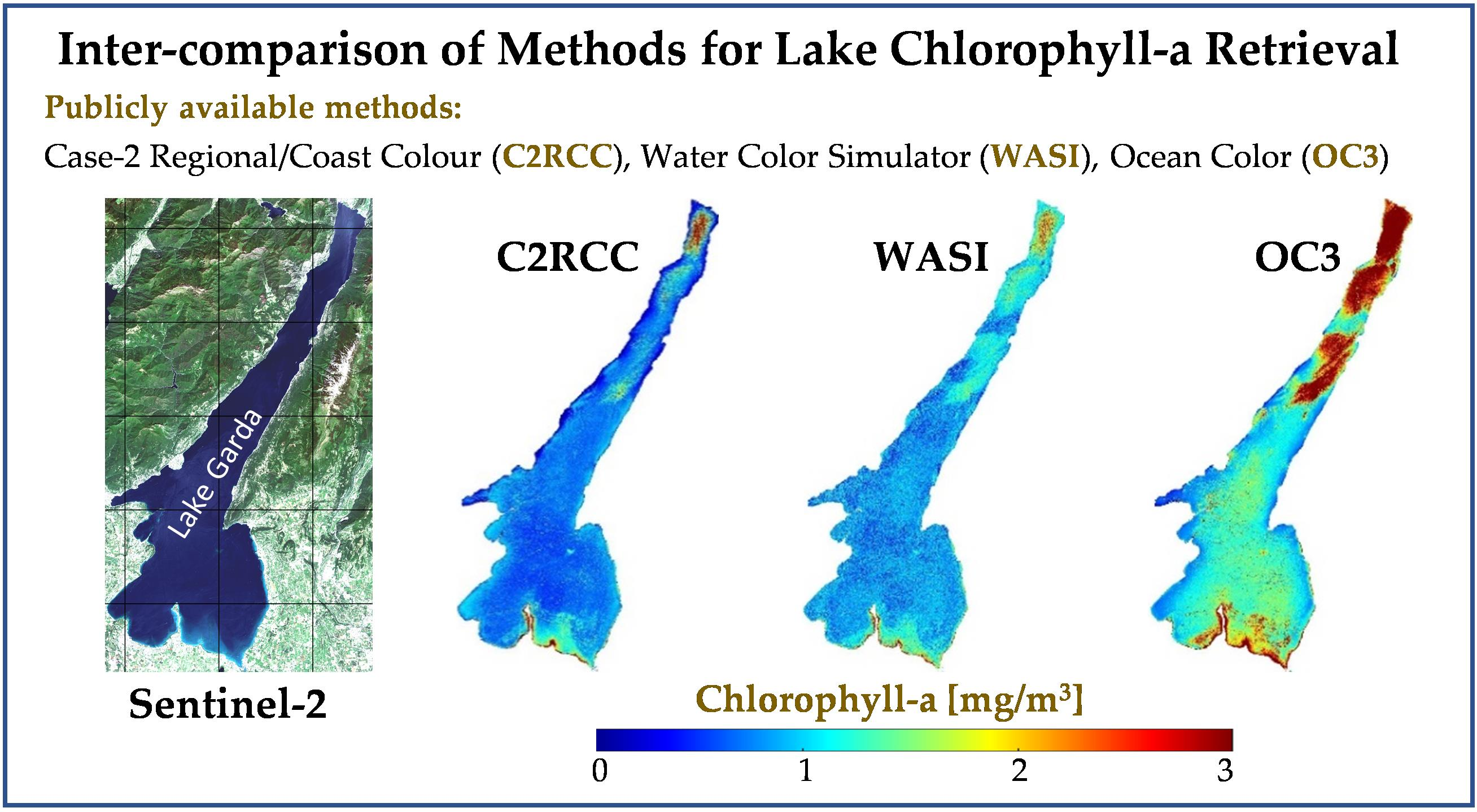
Given that current versions of C2RCC and WASI are relatively new tools available to the public, their applications in inland waters are yet scarce, and there is not yet available any comparison between their products. Moreover, OC3 is being used also in optically complex waters for retrieving the Chl-a concentration [37,38]. Thus, there is a need to perform a comparative analysis among the three methods to better understand the effectiveness of each processor in retrieving water quality parameters over lakes with different bio-optical conditions. The main goal of this study is to perform such cross-method comparison for evaluating the retrievals of Chl-a for which in situ matchup data are also available from Italian lakes. Complementary to our Chl-a analyses, relative comparisons are performed for all constituents including TSM and CDOM retrievals of C2RCC and WASI. In this regard, the following objectives are pursued: (i) demonstrating the utility, challenges, and performance of publicly available methods (C2RCC, WASI, and OC3) in retrieving Chl-a concentration of lakes; (ii) analyzing the cross-method consistency of Chl-a and other constituents (TSM and CDOM), and (iii) demonstration of the potential of Sentinel-2 (MSI) imagery in multitemporal retrieval of the mentioned constituents in lakes.

Section 2 introduces the studied lakes and datasets. Section 3 describes C2RCC, WASI, and OC3 methods and compares their characteristics. A set of metrics for accuracy and consistency assessments are also described. The results and discussions are provided in Section 4 and Section 5, respectively. The conclusions and outlooks are given in Section 6.

2. Studied Lakes and Datasets

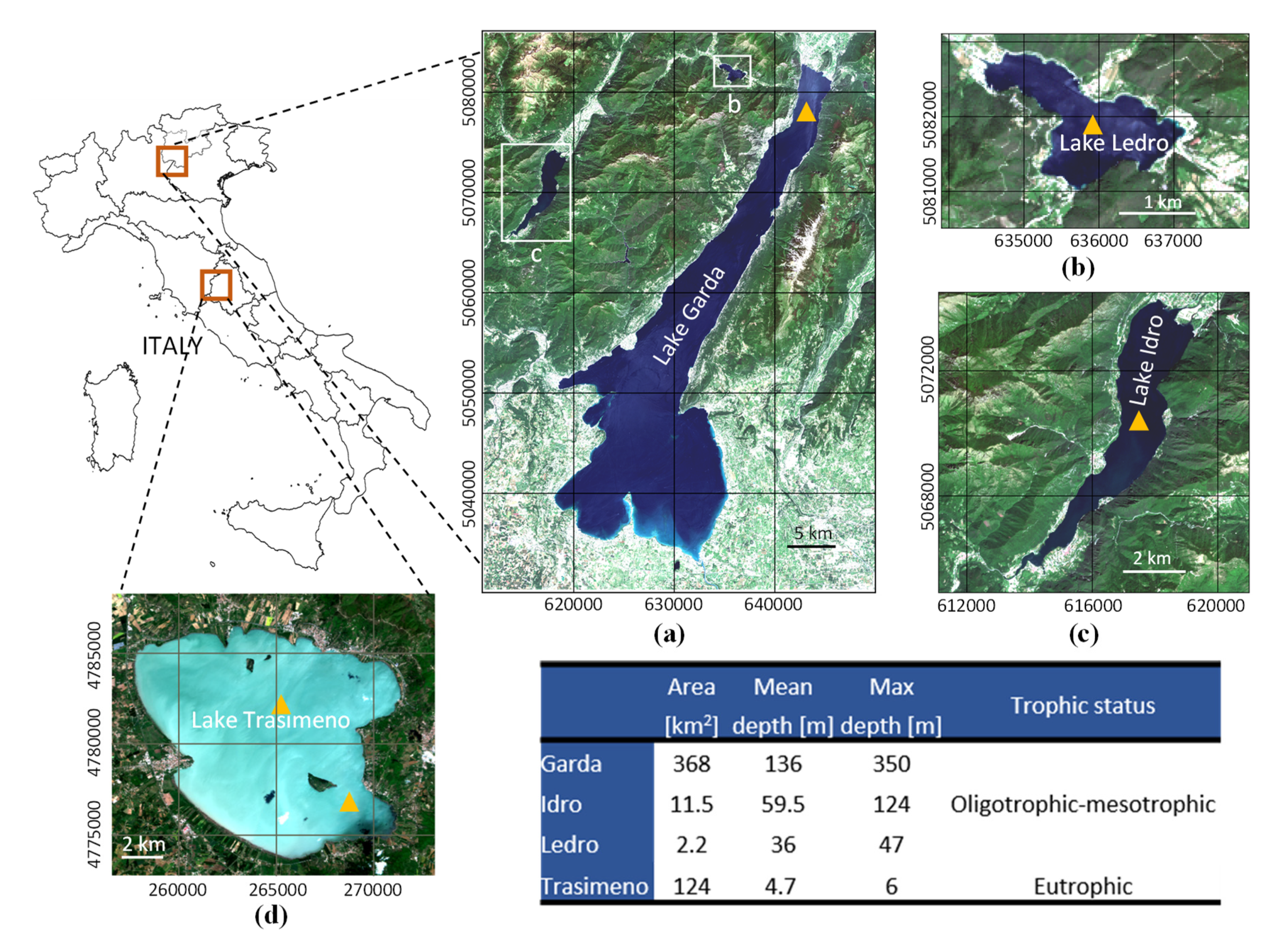
We have considered three subalpine lakes including Garda, Idro, and Ledro in northern Italy as well as a turbid lake in Central Italy (Trasimeno) for evaluation of the water quality retrieval algorithms in a multitemporal analysis framework (Figure 1). The studied lakes are considered as case II waters with complex optical properties [39,40]. Lake Garda (Figure 1a) is the largest lake in Italy. It is a key source of drinking and agricultural water and hydropower production. The main inflow of Lake Garda is the Sarca River in the northern part of the lake. Lakes Ledro (Figure 1b) and Idro (Figure 1c) are smaller lakes close to Lake Garda. The Chl-a concentration is low in these subalpine lakes and particularly in Lake Garda (<2.5 mg/m³ since 2012, [41]) and TSM < 15 g/m³ and $a_{CDOM}\left(440\right)$ < 1.1 m⁻¹ [42]. Lake Trasimeno (Figure 1d) has different bio-optical conditions than the other lakes. It is a shallow (depth < 6 m), turbid (Secchi depth ≈ 1.1 m), and eutrophic lake. Long-term measurement of Chl-a shows a range of 2 to 40 mg/m³ in two stations in the lake (Figure 1). The average TSM is about 10 g/m³ [40], and a mean value of 0.3 m⁻¹ can be considered for $a_{CDOM}\left(440\right)$ [43]. The southeast corner of Lake Trasimeno is colonized by aquatic vegetation. Seasonal algal blooms occur in the lake mostly in the period between July to September [40,43]. The selected lakes cover a relatively broad range of bio-optical conditions (from oligotrophic-mesotrophic to eutrophic) [44,45] that provide a comprehensive dataset for our inter-comparison analyses (Figure 1). They are optically deep, so the target methods are all applicable.

2.1. Sentinel-2 Imagery

Forty and 23 scenes (in total 63) with minimal cloud cover (<5% within the frame) from Sentinel-2A and Sentinel-2B, respectively, are selected for the subalpine lakes for a multitemporal analysis spanning from July 2016 to September 2019. The joint use of Sentinel-2A and Sentinel-2B data allows for denser temporal analysis and increasing the number of in situ matchups. Each image covers all three subalpine lakes. Seventeen cloud-free images (12 from Sentinel-2A and 5 from Sentinel-2B) of Lake Trasimeno are also available with corresponding in situ Chl-a data. Since most of the water quality relevant bands (< 1000 nm) are acquired at either 10 or 20 m, level-1C images are resampled to 20 m spatial resolution. Downsampling of the bands with 10 m resolution to 20 m enhances the signal-to-noise ratio and tends to enhance the retrievals.

The atmospheric correction is performed by the C2RCC processor, which provided accurate remote sensing reflectance (R_rs) in previous studies [34,46,47]. Apart from the demonstrated high quality of R_rs derived from C2RCC, it should be noted that the publicly available version of C2RCC works only with the built-in atmospheric correction. Thus, to make results consistent and comparable, the water quality retrieval methods are supplied with the same R_rs after C2RCC atmospheric correction. To ensure the reliability of input R_rs data, we investigated C2RCC’s quality flags [46] including (i) Rtosa_OOS: the input spectrum is out of the training range of the atmospheric correction neural net, (ii) Rtosa_OOR: the input spectrum is out of the training range of the atmospheric correction neural net, (iii) Rhow_OOS: the Rhow input spectrum to the inherent optical properties (IOPs) neural net is probably not within the training range of the neural net and the inversion is likely to be wrong, (iv) Rhow_OOS: one of the inputs to the IOP retrieval neural net is out of training range, and (v) Cloud risk: high downwelling transmission indicates cloudy conditions. None of the first four flags were raised for the analyzed images, indicating no issue identified by the processor regarding the quality of inputs to the atmospheric correction and IOP retrieval neural networks. We excluded the pixels with the cloud risk flag for all images. 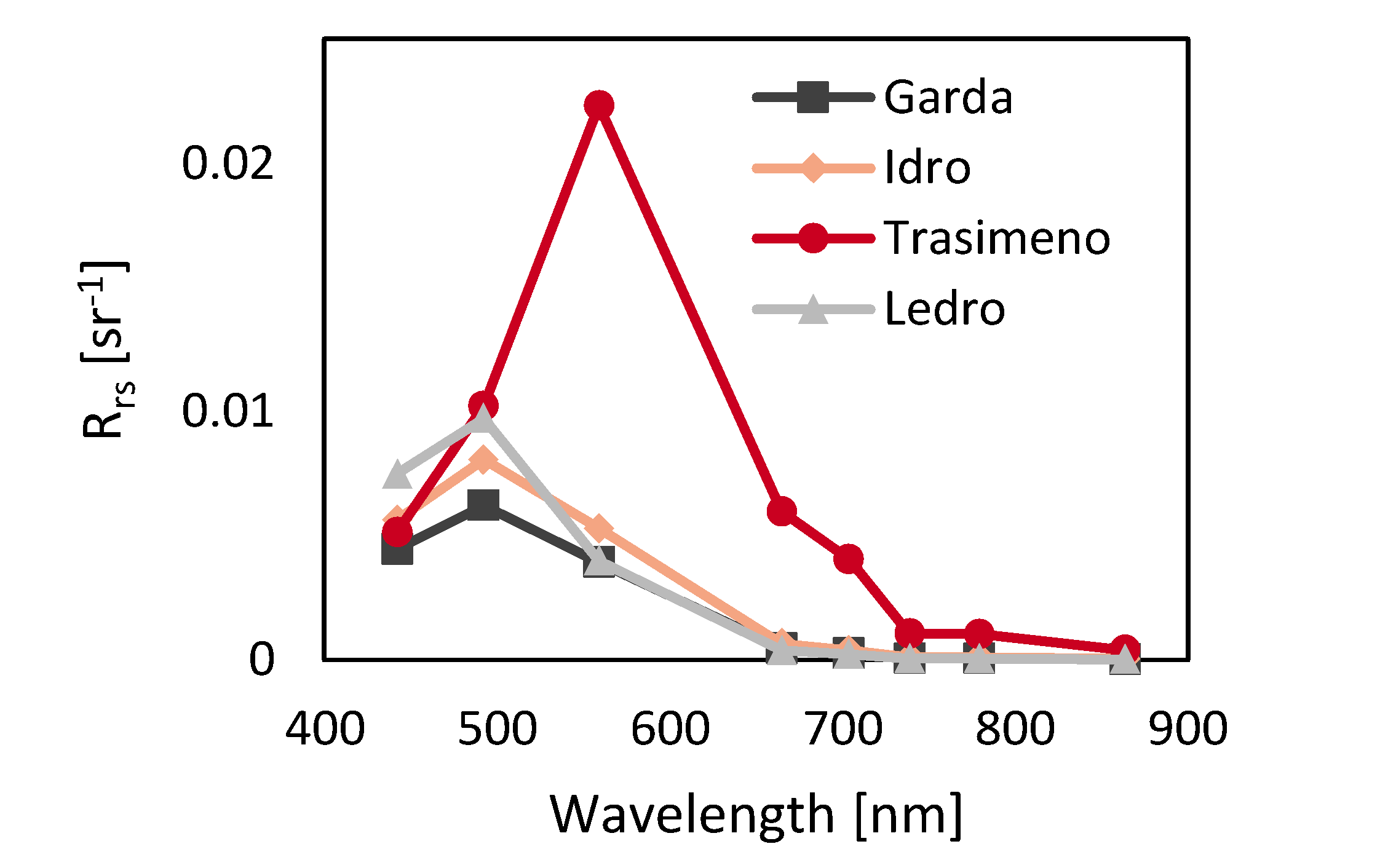Samples of R_rs spectra derived from the C2RCC atmospheric correction are illustrated in Figure 2. The spectra are provided for 8 July 2017 when all case studies are captured by Sentinel-2. Spatial windows (5 × 5 pixels) are applied to extract the average spectra at the location of stations (the central station for Trasimeno). As expected, Lake Trasimeno has very different optical characteristics from the others. In particular, the significantly higher R_rs across the spectrum (>500 nm) can be attributed to the higher TSM concentration [48] of Lake Trasimeno compared to the others.

2.2. In Situ Data

Twenty-eight samples were available from a measurement station in the northern part of Lake Garda (shown in Figure 1a). Furthermore, two stations in Lake Trasimeno (Figure 1d) provided 33 in situ matchups. Moreover, four and five in situ matchups were available from stations in Lake Idro and Ledro, respectively (Figure 1b,c). The measurements in Lakes Idro and Ledro are less frequent than the other lakes, and the availability of the data is further restricted by preserving a minimal time gap with the satellite overpass. The stations do not provide TSM and CDOM measurements. The image-derived values of Chl-a centered at the location of the stations are averaged for the matchup analyses [49]. The in situ concentration of Chl-a is measured based on spectrophotometric experiments following the standard methods [50,51]. The measurements in Lake Garda are all near simultaneous ($\pm 1$ h) with the Sentinel-2 overpasses. The measurements in other lakes are acquired within $\pm 2$ days on average from the satellite overpasses.f.

3. Methods

Although several algorithms exist for inversion of the water-leaving radiance [52,53], there are only a few available freely. In this study, the multitemporal dynamics of constituents are retrieved based on publicly available physics-based models of C2RCC and WASI. In addition, the semi-empirical OC3 algorithm is used for Chl-a estimation (

Table 1. Main characteristics of C2RCC, WASI, and OC3. TOA/BOA: top/bottom-of-atmosphere.

	Inversion Approach	Sensor Type	Input Spectral Data	Optical Depth of Water	Water Type	Sky/Sun Glint Correction
C2RCC	Neural networks	Pre-defined	TOA	Deep	Case-2	No
WASI	Analytical spectrum-matching	Independent	BOA	Shallow and deep	Case-1 and Case-2	Yes
OC3	Semi-empirical	Pre-defined	BOA	Deep	Case-1 and Case-2	No

The empirical methods are discarded in our inter-comparison analyses as gathering a sufficient amount of in situ data required for calibration of the regression model for each image is mainly infeasible when dealing with long time series. The methods are briefly discussed in the following subsections.

).

3.1. Case-2 Regional/Coast Colour (C2RCC)

The core of the C2RCC processor is based on inverting the top-of-atmosphere (TOA) radiance to water-leaving radiance (i.e., atmospheric part) and accordingly inverting the surface spectra to the IOPs of the water column (in-water part). The inversions are performed by means of a set of neural networks where the atmospheric and in-water parts are independent [17]. A large database (≈5 million) of radiative transfer simulations of water-leaving and TOA radiances in a range of IOPs are used to train the neural networks [17]. The simulations are performed by varying five IOPs including pigment absorption (a_pig), absorption of detritus (a_det), CDOM absorption ($a_{CDOM}$), scattering of white particles (b_wit) characterized by calcareous sediments, and typical sediment scatter (b_part). Two different optical conditions are assumed for the IOPs: (i) normal condition (C2RCC-N) in which all the mentioned IOPs vary in a relatively limited range, e.g., absorption of CDOM at 443 nm $a_{CDOM}$ < 1 m⁻¹, and (ii) extreme condition (C2RCC-E) in which IOPs span over a broad range including extreme conditions, e.g., $a_{CDOM}$ < 60 m⁻¹ (

Table 2. The range of IOPS considered in training C2RCC neural networks [17].

	apig [m−1]	adet [m−1]	${\mathit{a}}_{\mathit{C}\mathit{D}\mathit{O}\mathit{M}}$ [m−1]	bwit [m−1]	bpart [m−1]
C2RCC-N	[≈0, 5.3]	[≈0, 5.9]	[≈0, 1]	[≈0, 60]	[≈0, 60]
C2RCC-E	[≈0, 51]	[≈0, 60]	[≈0, 60]	[≈0, 590]	[≈0, 590]

).

Then, the retrieved IOPs are converted to the concentration of constituent by applying conversion factors. The TSM estimation involves scaling factors for b_part and b_wit termed as fac_b_part and fac_b_wit, respectively (Equtation (1)). Chl-a exponent (exp_Chl) and factor (fac_Chl) are used to convert a_pig to the Chl-a concentration (Equtaion (2)). Although C2RCC was originally developed as the MERIS case 2 water algorithm [54], major improvements are introduced in the current version available through ESA’s Sentinel Toolbox SNAP [55]. In this context, the recent C2RCC processor incorporates revised and extended neural networks, and it allows for processing the Sentinel-2 imagery. C2RCC is employed also for the generation of standard ESA Case-2 water products from Sentinel-3 (OLCI) imagery [17]. The C2RCC can be applied to the TOA radiance data of predefined sensors (OLI, MSI, etc.).

$$TSM=b_{part}\times fac\_b_{part}+b_{wit}\times fac\_b_{wit}$$

(1)

$$Chl={a_{pig}}^{exp\_Chl}\times fac\_Chl$$

(2)

3.2. Water Color Simulator (WASI)

The WASI processor [56] is capable of performing both forward and inverse modeling, i.e., simulation of water-leaving spectra and estimation of IOPs/constituents from spectral data, respectively. The inversion of the imagery data is implemented as a module called WASI-2D [18] (hereafter, we refer to WASI for brevity). WASI can be adapted to any multi- and hyper-spectral sensor and any aquatic environment including oceanic, coastal, and inland waters (case-1 and case-2 waters). The inverse modeling involves well-established analytical approaches and can be applied to the bottom-of-atmosphere (BOA, i.e., atmospherically corrected) imagery. In this context, WASI minimizes the mismatch between observed (image) and simulated spectrum by varying a set of parameters defining the shape and magnitude of the simulated spectra. The fitting procedure requires initialization of the variable parameters, which can be defined based on any pre-knowledge about the optical conditions and/or according to the user’s pre-fit exercises (the detailed descriptions are provided in the user manual of WASI [18]). Then, WASI examines the goodness of fit of the observed spectrum versus simulated spectrum for a maximum number of radiative transfer simulations in a given range of variable parameters. The outputs for a given input spectrum/pixel encompass the magnitudes of variable parameters associated with the simulated spectrum, which provides the best fit among the others. The goodness of fit is quantified based on the residuals of spectrum matching and also spectral angle as a measure of how good the spectral shapes match [57]. WASI performs this analysis on a pixel-by-pixel basis to retrieve the water quality parameters of the entire water body. Although a variety of parameters can be varied through the fitting procedure of WASI, by default, four parameters are set as standard variable parameters for analyzing optically deep waters. These parameters are (1) the concentration of a phytoplankton class (Chl-a) among six different classes available in WASI [57], (2) the concentration of TSM, (3) the absorption coefficient of CDOM at 440 nm $a_{CDOM}\left(440\right)$, and (4) the sun glint parameter $g_{dd}$. The parameter $g_{dd}$ is to compensate the artifacts on the water-leaving radiance due to sun glint (i.e., direct reflections from the water surface) and atmospheric effects. Further parameters characterize other IOPs (such as the spectral slope of CDOM absorption) as well as the artifacts from the water surface and atmospheric effects, which can be considered as variable or fixed parameters depending on the site-specific conditions. WASI allows for wavelength-dependent modeling of sun and sky glints at the water surface as well as phytoplankton classification using up to six species simultaneously through the bio-optical modeling [18,56,58]. WASI is a standalone and publicly available software [59]. The applicability of WASI in terms of the range of the constituents is provided in

Table 3. The applicability of WASI in terms of the range of constituents [60].

	Chl-a [mg/m3]	TSM [g/m3]	${\mathit{a}}_{\mathit{C}\mathit{D}\mathit{O}\mathit{M}}$ [m−1]
WASI	[≈0.5, 100]	[0.5, 50]	[0.05, 5]

.

3.3. Ocean Color (OC) Algorithm for Chl-a Estimation

The general form of the OC algorithm is a fourth-order polynomial expression relating a blue-green band ratio to the concentration of Chl-a [15,16]. The blue wavelength is considered as the maximum R_rs value within the blue (and slightly toward the green) portion of the spectrum, and the green wavelength refers to a spectral band located within 545 and 570 nm [15]. Therefore, more than two bands can be involved through retrieving the Chl-a depending on the band designation of the desired sensor. For instance, a traditional SeaWiFS OC algorithm incorporates three spectral bands centered at 443, 490, and 510 nm as candidate blue bands along with the one at 555 nm as the green band. This algorithm is called OC4, as four bands are involved in total. Recently, OC5 and OC6 algorithms [15] are also proposed for SeaWiFS by involving a short wavelength blue band (412 nm) as well as a red band (670 nm). In this context, OC3 (three-band version) considers the maximum R_rs value of the bands centered near 443 nm and 490 nm as $R_{rs}\left({\lambda }_b\right)$, which is applicable on Sentinel-2 (MSI) data. To define the coefficients of the polynomial, coincident in situ measurements of Chl-a and R_rs data are employed from different available databases. The authors of [15] provided the latest version of tuned coefficients using a globally representative dataset [60]. The polynomial coefficients are given for the MSI sensor based on the three-band (OC3) maximum band ratio, i.e., R_rs(443 > 493)/R_rs(559):

$$\begin{gathered} {log}_{10}\left(Chl-a\right)=a_0+a_{1}X+a_2{X}^2+a_3{X}^3+a_4{X}^4,X={log}_{10}\frac{R_{rs}\left({\lambda }_b\right)}{R_{rs}\left({\lambda }_g\right)} \\ OC3 \left(MSI\right):a=\left[0.3308,-2.66837, 1.59899, 0.55248,-1.4876\right]. \end{gathered}$$

(3)

3.4. Products Accuracy and Consistency Analyses

A variety of analyses and indices are employed to examine the accuracy and cross-method consistency of water quality products. A recent study [49] suggests the use of a comprehensive set of metrics to evaluate the performance of water quality retrieval methods. Thus, along with commonly used least-square metrics of the coefficient of determination (R²) and root mean square error/difference (RMSE/RMSD), other metrics such as bias, mean absolute error (MAE), and win rate are employed [49]. Bias is an indicator of either the overestimation (bias > 1) or underestimation (bias < 1) of the retrieved values on average. A bias value close to the unity indicates that the estimates are less biased. For example, a bias of 1.3 indicates that the estimated values are on average 1.3 times (30%) greater than the observed values. MAE always exceeds unity, indicating the relative error of estimates. Bias and MAE are both calculated in log-transformed space to account for the proportionality of the errors with the concentration of the constituents [49]. These metrics are unitless, allowing for comparison of the errors and biases related to parameters with different measurement units. The win rate (percent wins) is a metric that accounts for the pairwise comparison of the estimated and observed values. For every estimation, the algorithm that provides the lowest absolute residual (observed—estimated) is the winner. Then, the total number of wins for an algorithm divided by the total number of estimated samples provides the win rate for that algorithm [49]. We consider relative standard deviation (RSTD) as a metric for quantifying the spatial variations of the constituents within a single map. The metrics are given in Equations (4)–(8) for a total number of n estimated values E_i with associated observed values O_i. Note that RMSD is calculated similarly to RMSE but considering the estimated values from another method instead of O_i, which is used for relative comparison of the methods.

$$R^2=\frac{{\sum }_{i=1}^n{\left(E_i-\overline{O}\right)}^2}{{\sum }_{i=1}^n{\left(O_i-\overline{O}\right)}^2}, \overline{O}=\frac{1}{n}{\displaystyle \sum }_{i=1}^n{O}_i$$

(4)

$$RMSE={\left(\frac{{\sum }_{i=1}^n{\left(E_i-O_i\right)}^2}{n}\right)}^{1/2}$$

(5)

$$bias={10}^{\frac{{{\displaystyle \sum }}_{i=1}^{n}lo{g}_{10}\left(E_i/O_i\right)}{n}}$$

(6)

$$MAE={10}^{\frac{{{\displaystyle \sum }}_{i=1}^n\left|lo{g}_{10}\left(E_i/O_i\right)\right|}{n}}$$

(7)

$$RSTD=\frac{Std}{\overline{E}}, Std={\left(\frac{1}{n-1}{\displaystyle \sum }_{i=1}^n{\left|E_i-\overline{E}\right|}^2\right)}^{1/2}, \overline{E}=\frac{1}{n}{\displaystyle \sum }_{i=1}^n{E}_i$$

(8)

We consider also a temporal coefficient of variation (CV) to quantify the rate of changes in the concentration of constituents over time. Temporal CV provides a metric for not only evaluating the temporal consistency of the products for the cross-method comparison but also showing the temporal behavior of constituents:

$$Temporal\_CV=\frac{St{d}_{temp}}{{\overline{E}}_{temp}}, St{d}_{temp}={\left(\frac{1}{T-1}{\sum }_{t=1}^T{\left|{\overline{E}}_t-{\overline{E}}_{temp}\right|}^2\right)}^{1/2}, {\overline{ E}}_{temp}=\frac{1}{T}{\sum }_{t=1}^T{\overline{E}}_t.$$

(9)

T is the total number of images. ${\overline{E}}_t$ denotes the spatially averaged estimation at time t.

3.5. Parametrization of C2RCC and WASI

Analyzing the multitemporal Sentinel-2A/B images of the subalpine lakes (63 scenes) by means of WASI, two different optical properties of the water column are identified for different dates: (i) low CDOM and (ii) high CDOM. The detection of the dates with relatively high CDOM occurred while processing the imagery with WASI, as the normal initialization of the parameters led to significant mismatches between the observed (image) and simulated spectra. Then, setting a higher initial value for $a_{CDOM}$ provided accurate fitting. The R_rs values over the visible bands are very low for high-CDOM cases that can be attributed to the strong absorption of CDOM at short wavelengths [5]. This physical interpretation confirms the choice of higher CDOM initialization for those dates. Moreover, considering $g_{dd}$ as an indicator of the quality of atmospheric and glint correction, the values of this parameter do not show any significant differences among high-CDOM and low-CDOM cases (average $g_{dd}$ of each image < 0.005 sr⁻¹). This further proves the dominant impact of CDOM on the water-leaving spectra for the high-CDOM cases. The estimation of constituents for the high-CDOM dates was problematic using the C2RCC-N. C2RCC-N provided extremely high Chl-a values for the identified high-CDOM cases, whereas $a_{CDOM}$ remained quite low. As mentioned before, the training of C2RCC-N has been based on $a_{CDOM}$ ranging from 0 to 1 m⁻¹, which is not suitable for high-CDOM cases. We examined C2RCC-E for these cases, and it provided relatively reasonable retrievals of Chl-a, although TSM and CDOM were more reasonable employing C2RCC-N in terms of the range of estimated values and the level of noise on the maps. Thus, C2RCC-E is used for Chl-a retrieval in high-CDOM cases, whereas the rest of retrievals are based on C2RCC-N. Note that $a_{CDOM}$ outputs of C2RCC and WASI are at 443 nm and 440 nm, respectively. However, we consider the effect of this small wavelength shift (3 nm) negligible on our results and analyses.

For Lake Trasimeno, we considered three different initial values for Chl-a based on a pre-fit analysis in WASI. This is because the range of variations of Chl-a is relatively high in Lake Trasimeno, and different initializations were required for the WASI-based inversion. We applied both C2RCC-N and C2RCC-E for retrieving the constituents in this lake. The initial values of fit parameters for WASI and also the conversion factors of the C2RCC are given in

Table 4. The initial values of fit parameters and conversion factors for WASI and C2RCC.

WASI			C2RCC
Fit Parameters	Initial Values		Conversion Factors	Fixed Values
	Subalpine Lakes	Trasimeno
Chl-a [mg/m3]	1	5, 12, 20	fac_bpart	1.31
TSM [g/m3]	1	7	fac_bwit	1.7
$a_{CDOM}$ [m−1]	0.2, 0.9	0.2	exp_Chl	1.04
S [nm−1]	0.014	0.014	fac_Chl	21
$g_{dd}$ [sr−1]	0.02	0.02

. We considered Chl-a concentration associated with the fifth phytoplankton class (i.e., green algae) available in WASI. The phytoplankton class is chosen based on a pre-fit analysis in WASI that provided the optimal matches between the observed and simulated spectra. It is worth noting that the impact of any possible difference in the species of phytoplankton on the spectral signature becomes more sensible when using hyperspectral data [61]. Thus, possible variations or differences of the phytoplankton class would have minimal impacts on our retrievals from multispectral imagery. The initial values of the fit parameters are considered based on pre-fit analyses and the knowledge about the characteristics of the lakes (Section 2). The C2RCC conversion factors are used to estimate the concentrations of TSM and Chl-a from associated IOPs. TSM-related factors are derived based on IOPs reported in the GLaSS report [42]. The estimation of $a_{CDOM}$ does not involve any conversion factor as a direct output of C2RCC.

4. Results

The results are presented for each of the lakes individually. As the main target parameter, Chl-a results and maps are presented in more detail with accuracy assessment using in situ matchups.

4.1. Constituent Retrievals in Lake Garda

The multitemporal profiles of retrieved constituents averaged over pixels that none of the quality flags (Section 2.1) raised are shown in Figure 3 and Figure 4 for Lake Garda. There are 12 dates identified with high CDOM concentration (Figure 4a). The Chl-a estimates based on C2RCC-N are overestimated for those dates and inconsistent with the results of WASI and OC3 (Figure 3a). Employing C2RCC-E for the high-CDOM dates, the Chl-a retrievals are in better agreement with those derived from WASI and OC3 (

Table 5. Agreement analysis of the average Chl-a retrieval in Lake Garda based on different algorithms. Comparisons are in terms of R² and RMSD by including/excluding the high-CDOM cases.

	R2		RMSD [mg/m3]
	Incl.	Excl.	Incl.	Excl.
C2RCC-N vs. WASI	0.35	0.74	0.30	0.09
C2RCC-NE vs. WASI	0.50	NA	0.26	NA
C2RCC-N vs. OC3	0.39	0.90	1.12	0.40
C2RCC-NE vs. OC3	0.65	NA	0.84	NA
WASI vs. OC3	0.20	0.75	1.28	0.63

). The estimates of CDOM and TSM based on C2RCC-E for high-CDOM dates were extremely unreliable (extremely large values and noisy maps), so we excluded them from the analyses. Note that C2RCC-NE indicates the use of C2RCC-N and C2RCC-E for low-CDOM and high-CDOM dates, respectively. C2RCC-N and WASI retrievals are in good agreement for TSM (Figure 4a) and CDOM (Figure 4b). The RSTD analyses indicate that C2RCC retrievals of Chl-a are extremely spread out around the average value (Figure 3b). The temporal average of the RSTD for C2RCC is 1.65, whereas it is much lower for WASI (0.63) and OC3 (0.80).

Table 6. Agreement of C2RCC-N and WASI in the estimation of TSM and CDOM in Lake Garda in terms of R² and RMSD by including/excluding the high-CDOM cases.

	R2		RMSD
TSM	Incl.	Excl.	Incl.	Excl.
	0.77	0.87	0.14 g/m3	0.10 g/m3
${\mathit{a}}_{\mathit{C}\mathit{D}\mathit{O}\mathit{M}}$	0.75	0.86	0.15 m−1	0.03 m−1

shows the agreement analysis between C2RCC-N and WASI for TSM and CDOM products in Lake Garda. As evident, the agreements associated with both TSM and CDOM are stronger than that of the Chl-a either including or excluding the high-CDOM dates. However, exclusion of the high-CDOM cases improves the agreements, e.g., 0.11 (15%) improvement of R² and 0.12 m⁻¹ (80%) improvement of RMSD for $a_{CDOM}$ estimates (Table 6). Figure 5 illustrates the temporal variations of the Chl-a derived from different methods at the measurement station in Lake Garda. The values are extracted by averaging over a window of 5 × 5 pixels centered at the station coordinates. The available in situ values are also plotted for comparison. The in situ measurements (Figure 5) further confirm that C2RCC-N extremely overestimates Chl-a for the high-CDOM dates (bias= 7.8), whereas other methods, particularly WASI, provide more reliable estimates.

Figure 6 shows retrieved-to-observed matchups of Chl-a in Lake Garda. The WASI-based estimates (Figure 6b) exhibit the highest correspondence (R² = 0.68). Although C2RCC-E provided more reliable estimates of Chl-a than C2RCC-N for the high-CDOM cases, the estimates are less accurate than those of WASI. This leads to lower accuracy of the C2RCC-NE (R² = 0.41, Figure 6a). OC3 provided less accurate retrievals than others (Figure 6c). The agreement of methods is strong excluding the high-CDOM cases (R² = 0.74, Table 5). The scatter plots (Figure 6) do not indicate any systematic pattern for each cluster of points associated with Sentinel-2A/B data. This is an indicator of consistent retrievals from the twin Sentinel-2 (MSI) sensors so that their joint use enhances the revisit frequency. The WASI-based estimates of Chl-a have a reasonable bias close to unity (0.91), indicating slight underestimation by 9% (Figure 6b), while C2RCC on average underestimates Chl-a by 22% (bias = 0.78, Figure 6a) and OC3 overestimates it by 27% (bias = 1.27, Figure 6c). Moreover, WASI leads to the lowest MAE and the highest win rate compared to the other methods. The win rate of OC3 is higher than C2RCC, although other accuracy metrics are in the favor of C2RCC (Figure 6).

Figure 7 illustrates examples of Chl-a maps derived from WASI, C2RCC-N, and C2RCC-E for a high-CDOM case (24 October 2018). As evident, the Chl-a map based on C2RCC-N is oversaturated with extreme values. Note that the range of the color bar is retained consistently for a better interpretation, but Chl-a values exceed 25 mg/m³. C2RCC-E leads to more realistic values of Chl-a than C2RCC-N though the resulting map is slightly noisy. Examples of multitemporal Chl-a maps are shown in Figure 8 for low-CDOM cases. The visual inspection implies that the multitemporal maps of WASI and C2RCC are in good agreement. The OC3 overestimates Chl-a compared to other methods, yet the spatial patterns of Chl-a are in good accordance, particularly with WASI. Multitemporal retrievals of TSM and CDOM in Lake Garda by means of C2RCC and WASI methods are shown in Figure 9 and Figure 10 for the dates of the Chl-a examples. Visual comparison of the corresponding maps for a given date reveals strong agreement of the maps, particularly for the CDOM parameter. Note that the shoreline pixels (shallow water) are excluded from the analyses.

4.2. Constituent Retrievals in Lake Ledro

C2RCC-E provided extreme values and noisy maps for all of the three constituents; therefore, it is dropped from further analyses. The temporal profiles of the Chl-a averaged over Lake Ledro are illustrated in Figure 11. The agreements of the average values of constituents retrieved by different methods in Lake Ledro are expressed in terms of R² and RMSD in

Table 7. Agreement analysis of Chl-a, TSM, and CDOM retrievals in Lake Ledro based on different algorithms. Comparisons are in terms of R² and RMSD.

	Chl-a [mg/m3]		TSM [g/m3]		${\mathit{a}}_{\mathit{C}\mathit{D}\mathit{O}\mathit{M}}$ [m−1]
	R2	RMSD	R2	RMSD	R2	RMSD
C2RCC-N vs. WASI	0.65	0.17	0.75	0.16	0.88	0.04
C2RCC-N vs. OC3	0.93	0.44	NA	NA	NA	NA
WASI vs. OC3	0.66	0.94	NA	NA	NA	NA

. There are strong agreements between the retrievals of C2RCC and WASI. The R² of $a_{CDOM}$ reaches 0.88, and there is a strong agreement for TSM retrievals (R² = 0.75). The agreements between different methods of Chl-a estimation are strong, although C2RCC-N vs. WASI yielded the lowest RMSD (0.17 mg/m³). In situ matchup analysis indicates the reliability of Chl-a retrievals and the high consistency of C2RCC (Figure 12a) and WASI (Figure 12b) retrievals. OC3 (Figure 12c) tends to overestimate the Chl-a concentrations (bias = 1.32).

Multitemporal examples of Chl-a maps are shown in Figure 13. The visual comparison indicates good agreement between the maps derived from different methods except for one case (28 November 2018) where the estimates of OC3 exhibit larger values.

4.3. Constituent Retrievals in Lake Idro

For Lake Idro, the Chl-a retrievals of C2RCC-NE are more comparable than C2RCC-N with those of WASI and OC3 (Figure 14). Quantitative assessment of the Chl-a estimates indicates a very strong agreement (R² > 0.7) among the methods by excluding the high-CDOM cases (

Table 8. Agreement analysis of the Chl-a retrieval in Lake Idro based on different algorithms. Comparisons are in terms of R² and RMSD by including/excluding the high-CDOM cases.

	R2		RMSD [mg/m3]
	Incl.	Excl.	Incl.	Excl.
C2RCC-N vs. WASI	0.32	0.72	0.27	0.16
C2RCC-NE vs. WASI	0.28	NA	0.28	NA
C2RCC-N vs. OC3	0.85	0.86	1.63	0.79
C2RCC-NE vs. OC3	0.22	NA	3.75	NA
WASI vs. OC3	0.50	0.70	3.01	1.16

). The in situ Chl-a matchups (low-CDOM cases) indicate the reliability of retrievals and high consistency among WASI (Figure 15b) and C2RCC (Figure 15a) products. The estimates of OC3 are largely biased (Figure 15c). The agreement metrics are estimated for TSM and CDOM retrievals as well (

Table 9. Agreement of C2RCC-N and WASI in the estimation of TSM and CDOM in Lake Idro in terms of R² and RMSD by including/excluding the high-CDOM cases.

	R2		RMSD
TSM	Incl.	Excl.	Incl.	Excl.
	0.64	0.71	0.23 g/m3	0.20 g/m3
${\mathit{a}}_{\mathit{C}\mathit{D}\mathit{O}\mathit{M}}$	0.72	0.76	0.18 m−1	0.07 m−1

). The agreement between the TSM temporal profiles is strong, either including or excluding the high-CDOM cases, though for the latter case, it is stronger. The estimates of CDOM are also in good agreement in terms of R² (0.72), even including the high-CDOM cases. However, excluding the high-CDOM dates, the RMSD reduces on the order of 60%.

A series of temporal Chl-a maps derived from the investigated methods are shown in Figure 16. The general patterns of the maps are comparable, although the WASI vs. C2RCC maps show stronger agreements. The OC3-based maps are mostly overestimated with respect to the two other methods.

4.4. Constituent Retrievals in Lake Trasimeno

Figure 17 shows the temporal profile of Chl-a averaged over Lake Trasimeno. The highest correlation is between C2RCC-E and WASI (

Table 10. Agreement among C2RCC-N, C2RCC-E, and WASI in the estimation of Chl-a, TSM, and CDOM in Lake Trasimeno in terms of R² and RMSD.

	R2			RMSD
	Chl-a	TSM	CDOM	Chl-a [mg/m3]	TSM [g/m3]	CDOM [m−1]
C2RCC-N vs. WASI	0.10	0.17	0.18	6.7	6.2	0.65
C2RCC-E vs. WASI	0.76	0.52	0.63	3.3	16.1	0.38
C2RCC-N vs. OC3	0.28	NA	NA	9.3	NA	NA
C2RCC-E vs. OC3	0.47	NA	NA	5.4	NA	NA
WASI vs. OC3	0.41	NA	NA	8.5	NA	NA

). The reduced R² of C2RCC-N can be attributed to a better adaptation of C2RCC-E for turbid and optically complex lakes such as Trasimeno. C2RCC-E provides stronger agreements than C2RCC-N with both WASI and OC3. For instance, the RMSD of Chl-a for C2RCC-E vs. WASI is 3.4 mg/m³ lower than that of C2RCC-N vs. WASI (Table 10). Note that the estimates for the southeast corner of the lake (open bay) and the shorelines are excluded from the averaging.

Samples of multitemporal Chl-a maps derived in Lake Trasimeno based on different methods are shown in Figure 18.

The matchup analyses show the outperformance of WASI in the estimation of Chl-a in Lake Trasimeno (Figure 19). Similar to the results derived for the subalpine lakes, OC3 retrievals are highly overestimated (Figure 19c). WASI-based estimates of Chl-a provided lower bias and MAE compared to other methods (Figure 19b). The win rate of WASI is also ≈20% higher than C2RCC-E (Figure 19a,b). On average, OC3 estimates are ≈2.3 times higher than the in situ data.

4.5. Temporal Variation of the Constituents

The temporal variations of the constituents are quantified in terms of temporal CV (

Table 11. Temporal CV of the constituents derived from different methods.

	Chl-a			TSM		${\mathit{a}}_{\mathit{C}\mathit{D}\mathit{O}\mathit{M}}\left(440\right)$
	C2RCC	WASI	OC3	C2RCC	WASI	C2RCC	WASI
Garda	0.79	0.36	0.76	0.44	0.39	0.88	1.28
Ledro	1.23	0.39	1.37	0.74	0.50	1.69	1.57
Idro	1.4	0.31	0.61	0.59	0.53	0.94	1.25
Trasimeno	0.52	0.67	0.41	0.30	0.31	0.54	0.76

). The WASI-based retrievals provided more plausible temporal CVs for the subalpine lakes given the vicinity and similar characteristics of these lakes. In the three subalpine lakes, the temporal CV of Chl-a is about 0.35 based on WASI estimates, which is almost half that of Lake Trasimeno. Given the low concentration of Chl-a in the subalpine lakes, this rate of variation has no significant impact on the Chl-a concentration, which is in line with the available information [41]. The higher variation of Chl-a in Lake Trasimeno is also indicated in previous studies [40]. Higher concentrations of Chl-a (algal blooms) are identified in September 2016 and September 2018 (Figure 17). Thus, WASI-based retrievals captured the temporal trend of the constituents that is more plausible.

4.6. Computational Time of the Methods

WASI is time demanding for large lakes such as Garda, whereas the processing time for small lakes (Idro and Ledro) is more comparable with the other methods (

Table 12. The computational time of different methods for a single image.

	WASI	C2RCC	OC3
Garda	≈16 h	≈5 min Atmospheric correction and retrieval of constituents for three lakes	≈1 min Chl-a retrieval for three lakes
Idro	≈30 min
Ledro	≈6 min
Trasimeno	≈7 h	≈2 min	<1 min

). The methods are implemented on a computer with an Intel Xeon 3.8 GHz quad-core processor and 64 GB RAM. This allowed us to run six WASI instances in parallel on the single machine without any interruption, which reduced the computational time about six times. It should be noted that Sentinel-2 imagery can be down-sampled to a coarser resolution depending on the application (e.g., 60 m) for large lakes such as Garda. This will reduce the computational time by a factor of 3 × 3 = 9.

5. Discussion

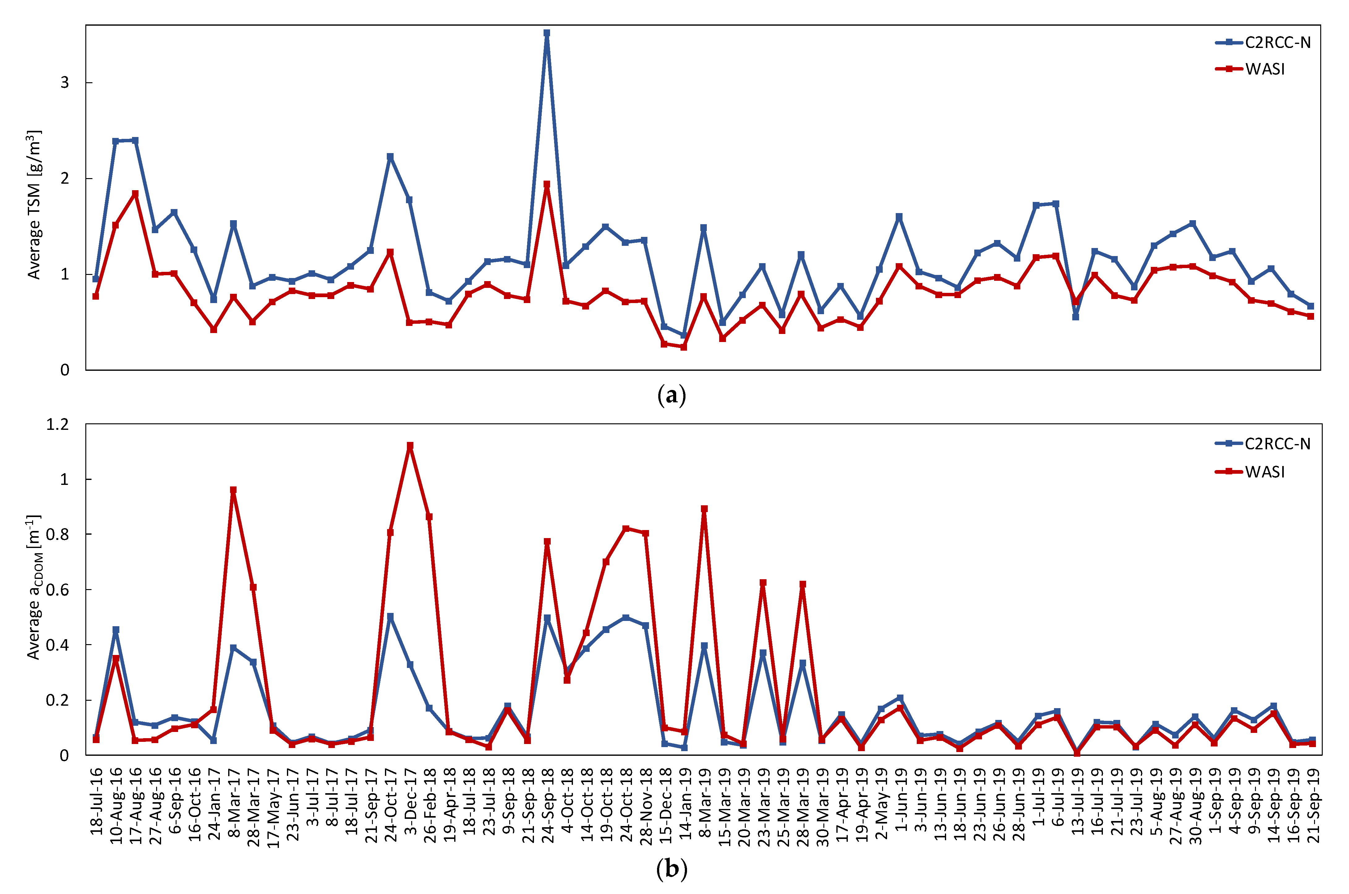
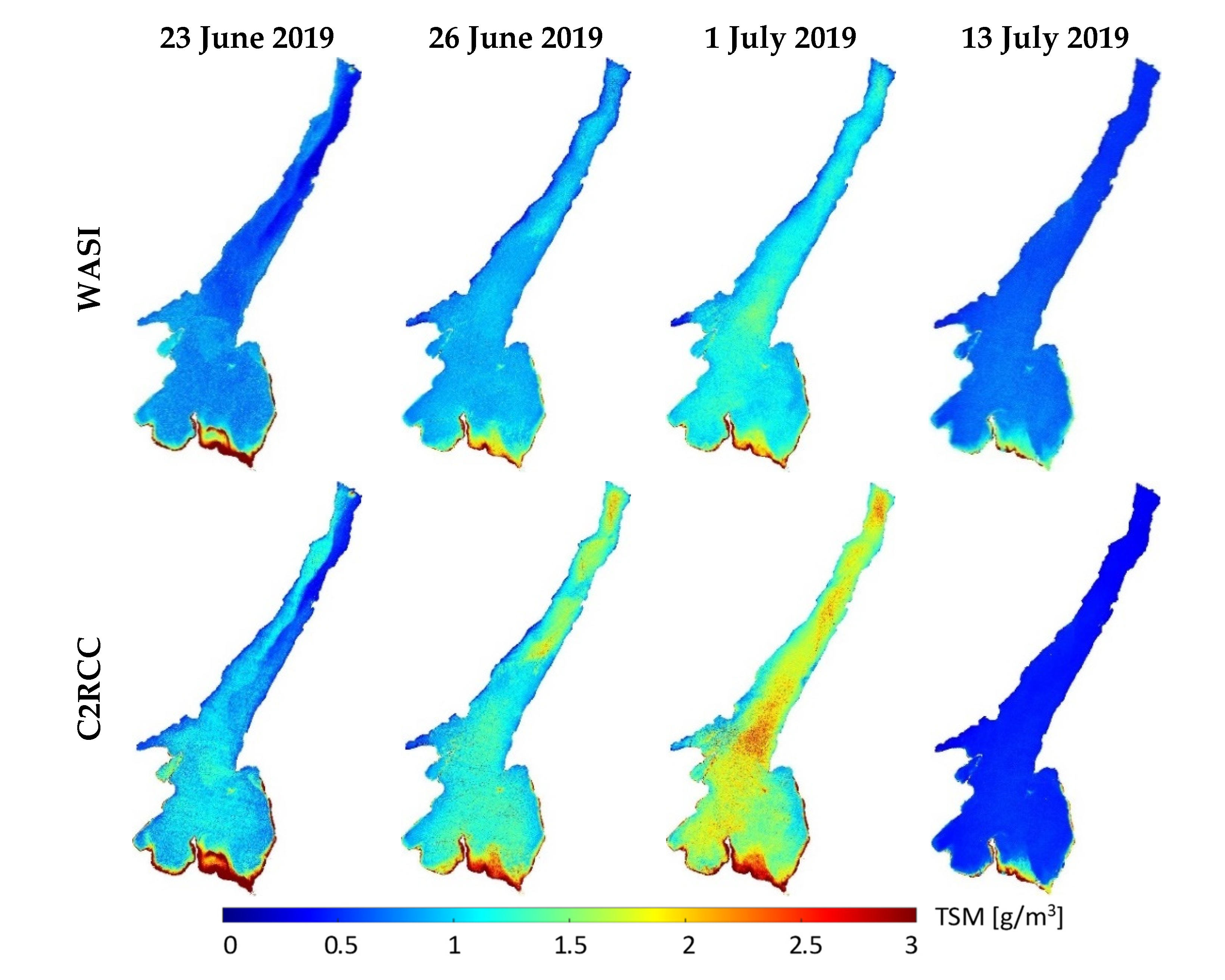
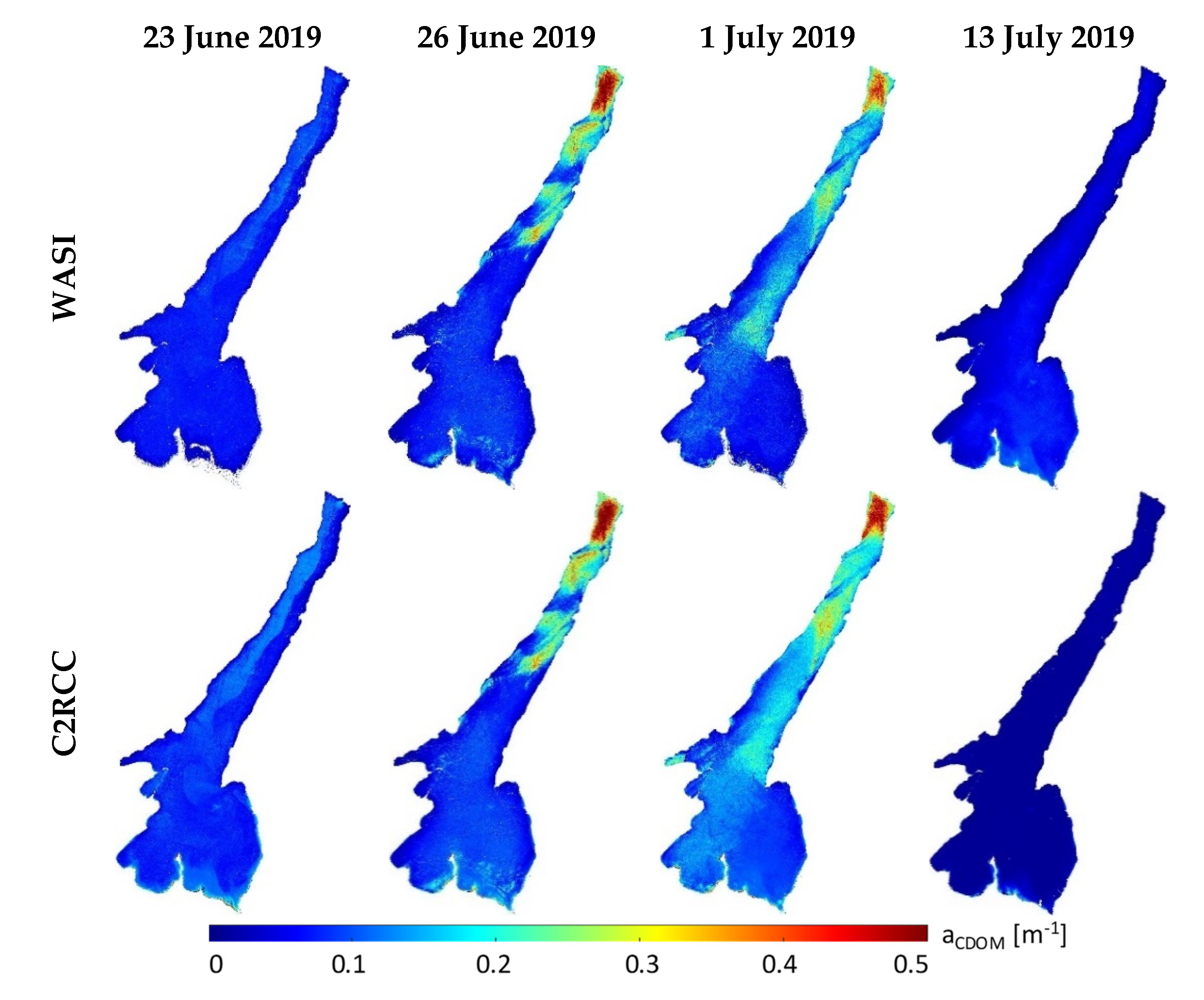
In this study, the freely available inversion methods of C2RCC and WASI, as well as the semi-empirical OC3 method, are examined and compared through processing a long time-series of Sentinel-2 imagery acquired over different bio-optical conditions. In the subalpine lakes, C2RCC and WASI provided products with high consistency over low-CDOM cases ($a_{CDOM}$< 0.5 m⁻¹). Although in situ matchup validation is performed only for Chl-a (the main goal of the study), the high consistency of the derived TSM and CDOM concentrations and their spatial distributions derived from two independent methods indicates their reliability also for these parameters. Given the very different inversion approaches of C2RCC and WASI, it is unlikely that there is a systematic error that affects both methods in the same way. 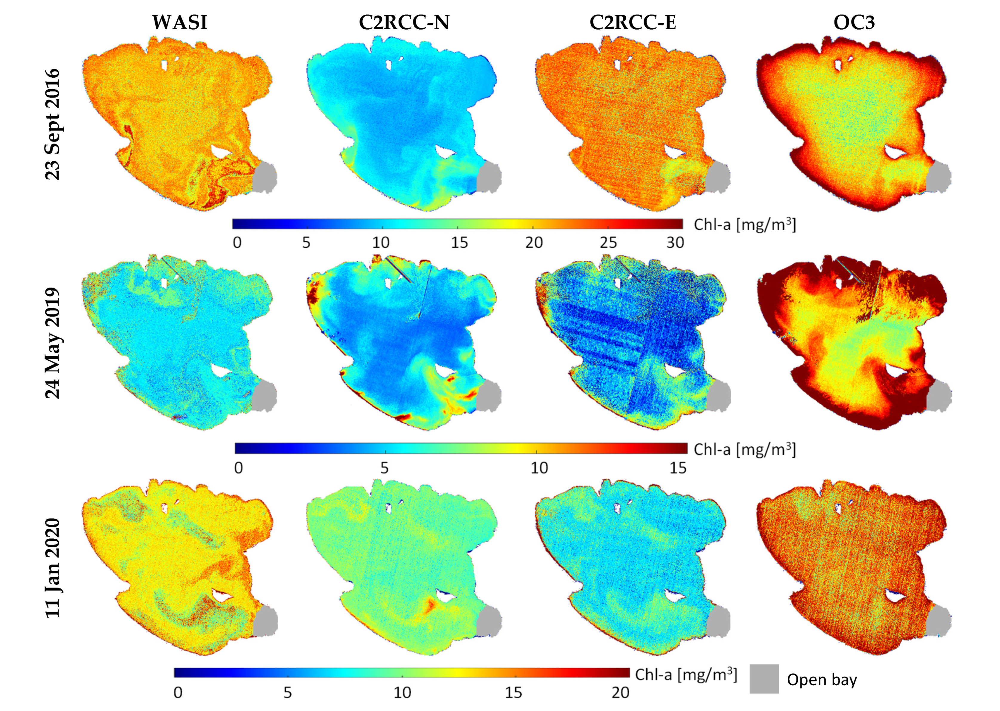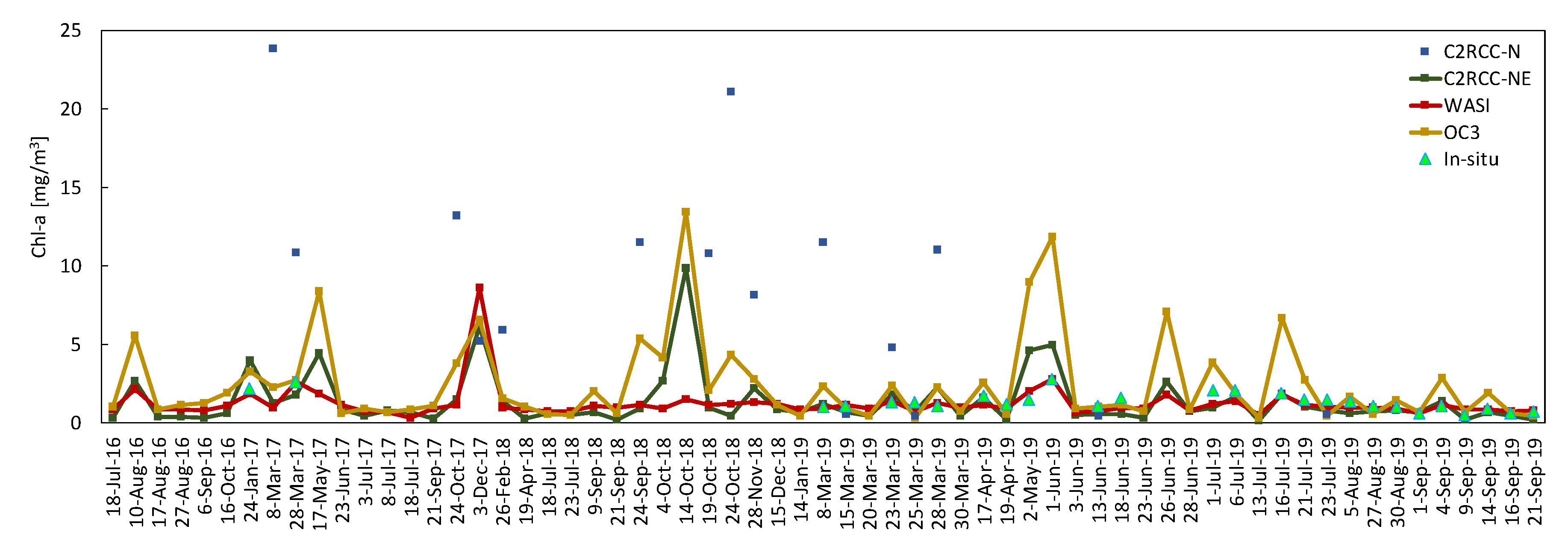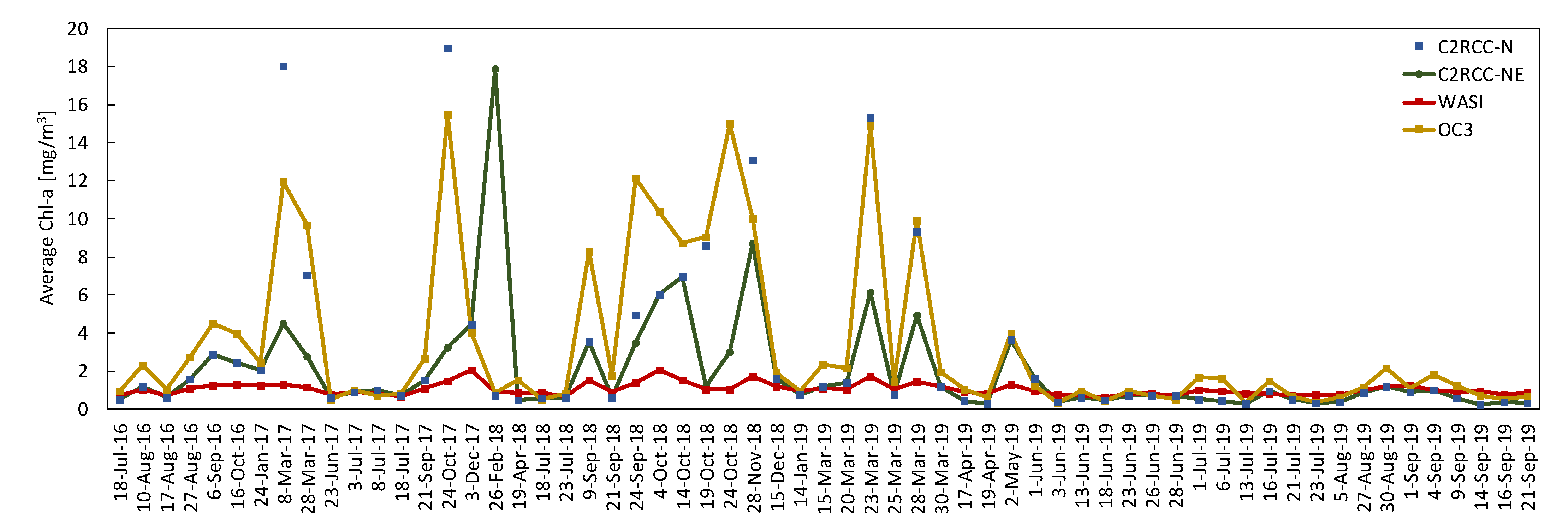Moreover, the ranges of parameters agree well with the available information from the studied lakes (Section 2). This is also in line with the in situ Chl-a data. The comparison of methods and in situ matchups from Lake Garda reveal unrealistic high Chl-a estimates of C2RCC-N when WASI-based $a_{CDOM}$ is relatively high. The Chl-a values based upon C2RCC-N exceed 25 mg/m³ for the high-CDOM cases (Figure 5 and Figure 7), which is much higher than the values reported in a recent study in Lake Garda (< 2.5 mg/m³) over the studied period [41]. A visual inspection of Figure 4 conveys that temporal trends of average TSM and CDOM derived from WASI and C2RCC-N are in good agreement in Lake Garda. The large mismatches are again related to high-CDOM cases. The training of C2RCC-N has been based on relatively low values of $a_{CDOM}$(< 1 m⁻¹), whereas according to the long-term observations, this parameter can reach values above 1.2 m⁻¹ in Lake Garda [42]. 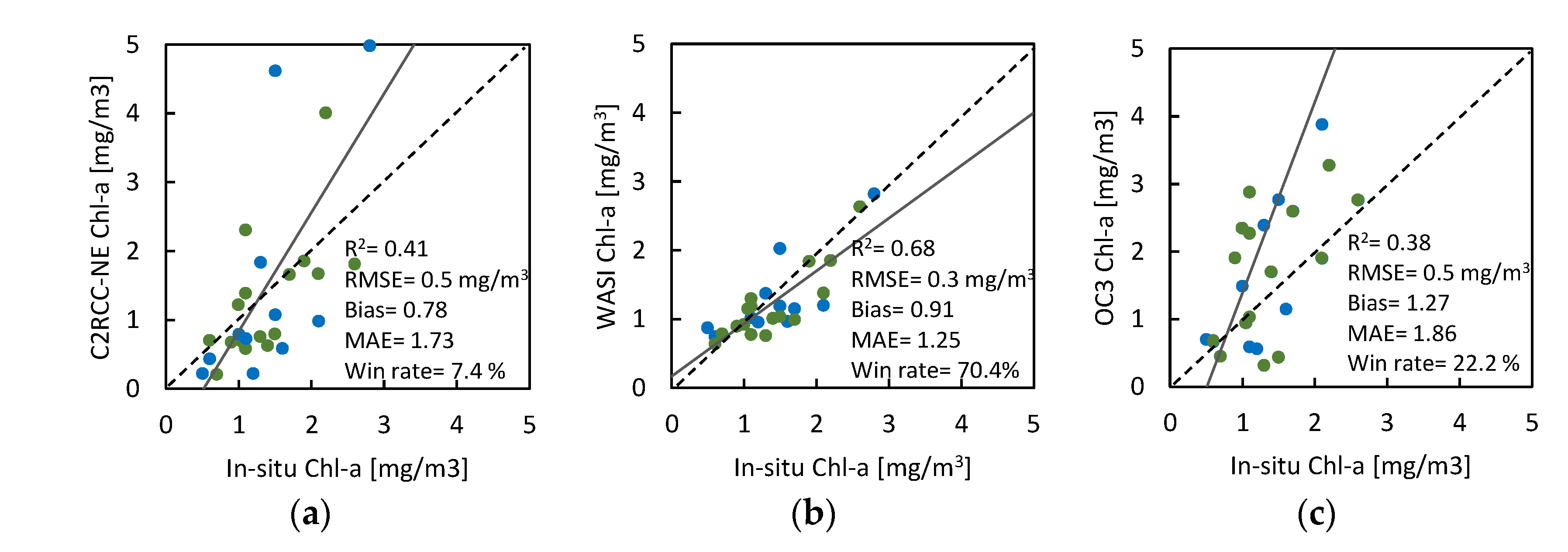The limited range of $a_{CDOM}$ considered through training the C2RCC leads to an underestimation of this parameter for the high-CDOM cases. 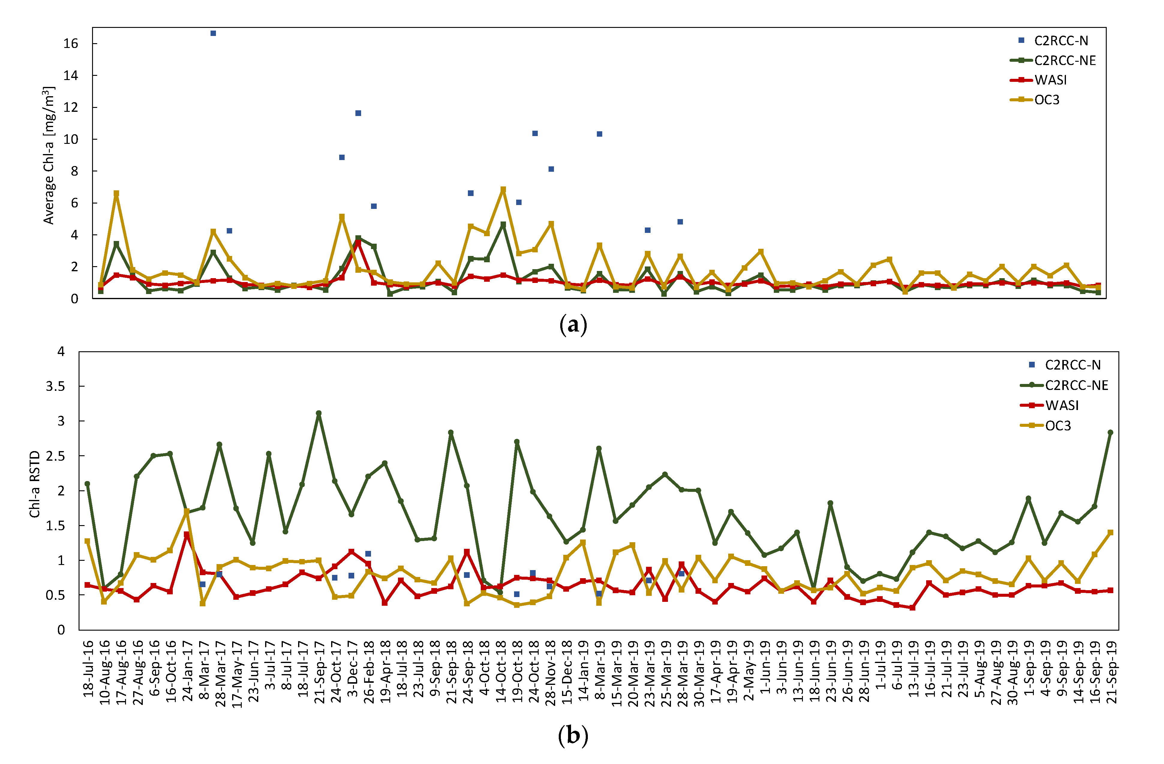Excluding the high-CDOM cases leads to a remarkable enhancement of the agreements, e.g., improvement of Chl-a R² on the order of 0.39 and RMSD of 0.21 mg/m³ comparing C2RCC-N against WASI. 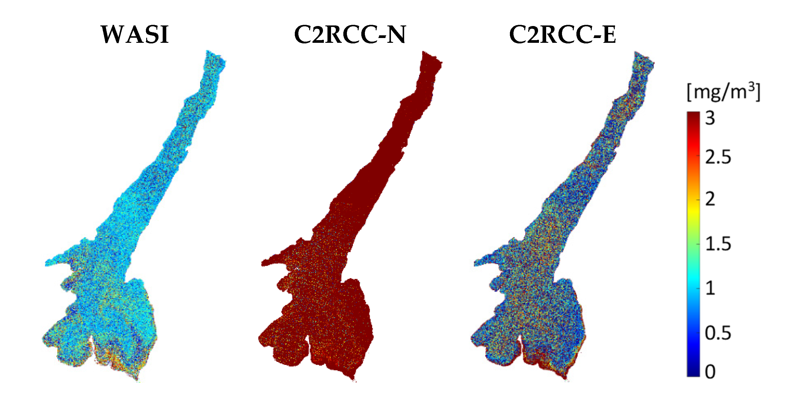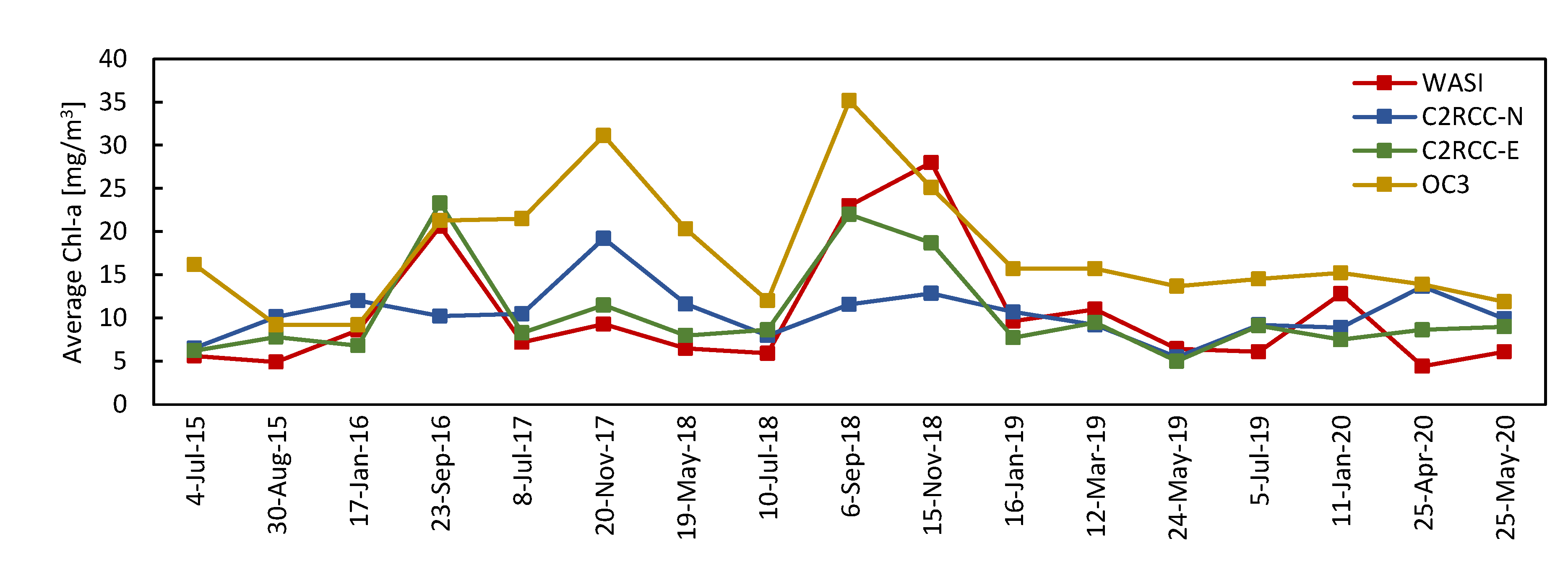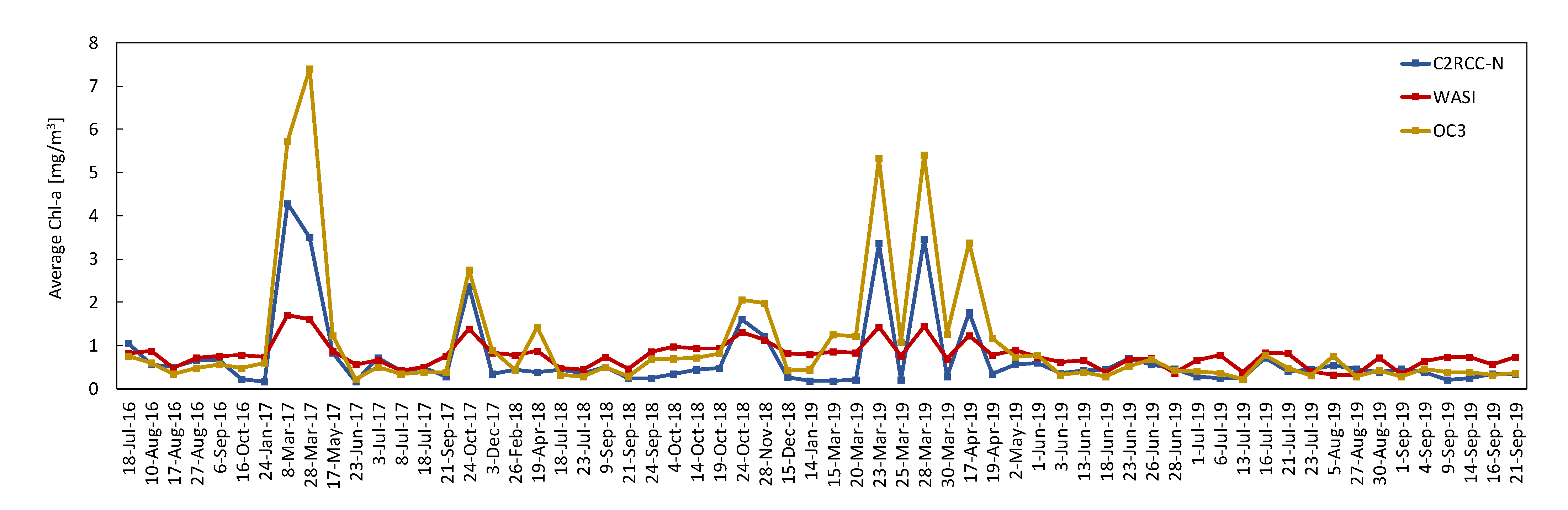According to a previous long-term study of Chl-a, it can be inferred that the spatiotemporal RSTD does not exceed 0.8 within three representative stations considered over Lake Garda [42]. This serves as a proxy that the RSTD values of WASI and OC3 are more reliable than those of C2RCC. In Lake Ledro, the largest discrepancies among retrievals of methods are again associated with relatively higher values of CDOM. The differences are not as large as those for the high-CDOM cases of Lake Garda. However, this indicates a potential confusion between CDOM and Chl-a spectral characteristics while processing the data with C2RCC. 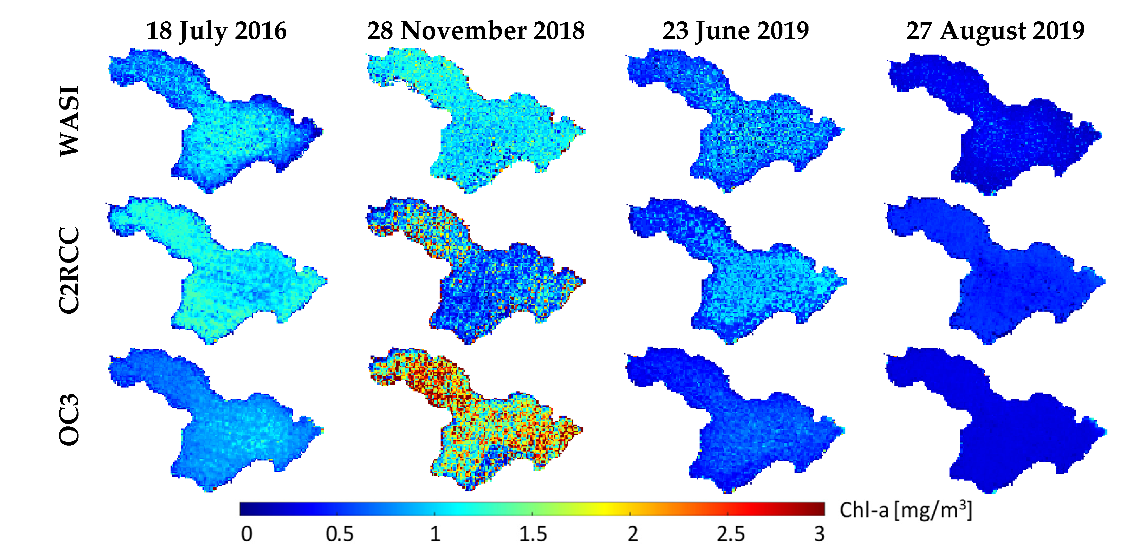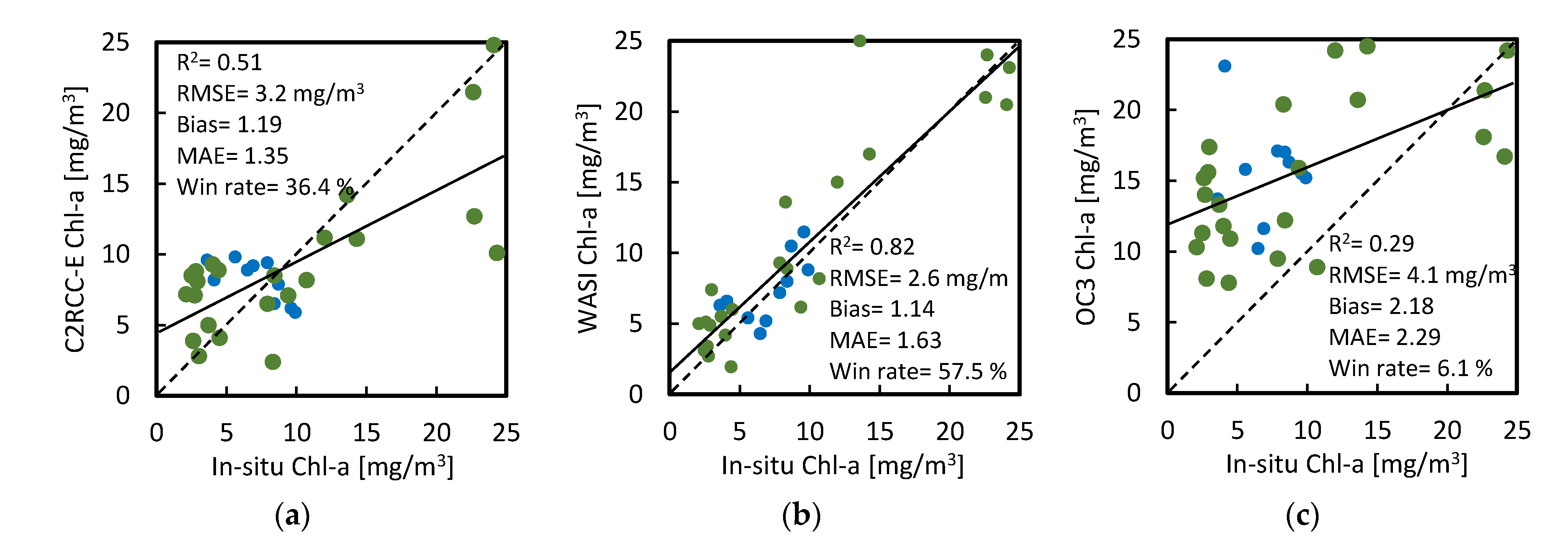The temporal profile of average Chl-a for Lake Idro is in line with the results from Lake Garda, which confirms that retrievals of Chl-a based on C2RCC-N are problematic (extreme values) for high-CDOM cases (Figure 14). Although C2RCC-E provided more reliable estimates of Chl-a for the high-CDOM cases, the retrievals of CDOM and TSM were problematic (extreme values and noisy maps). 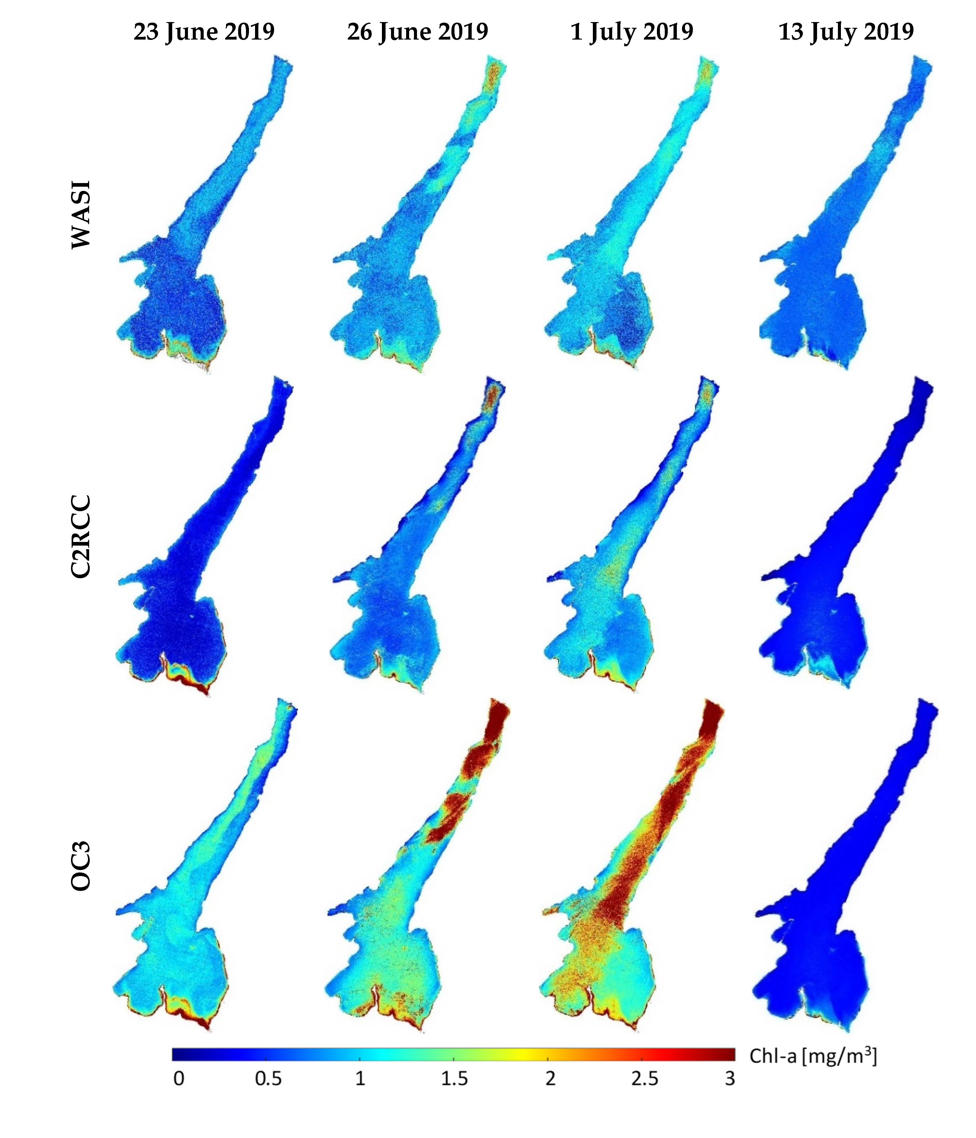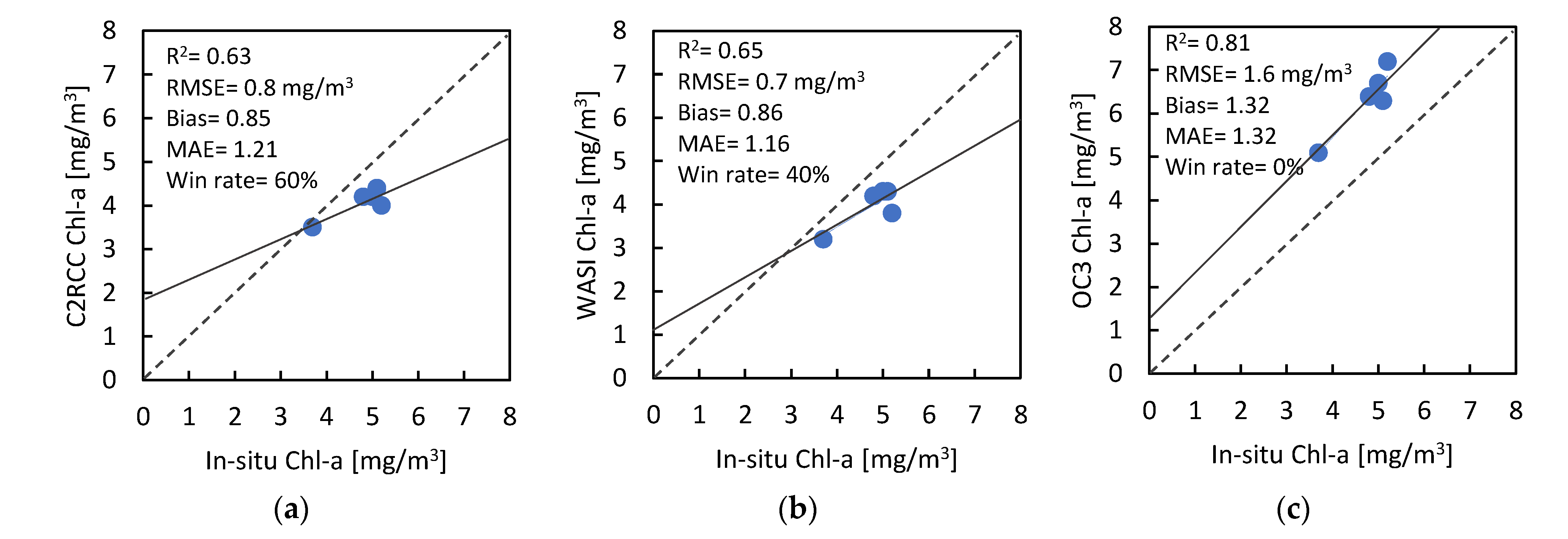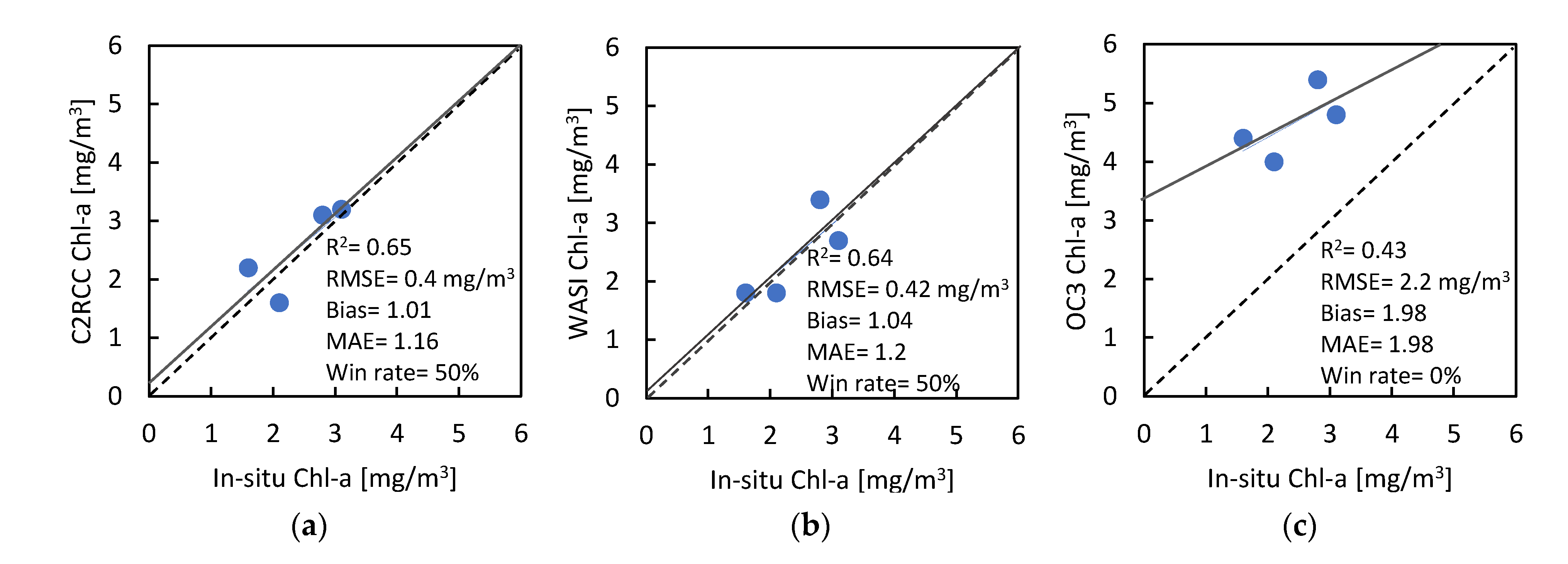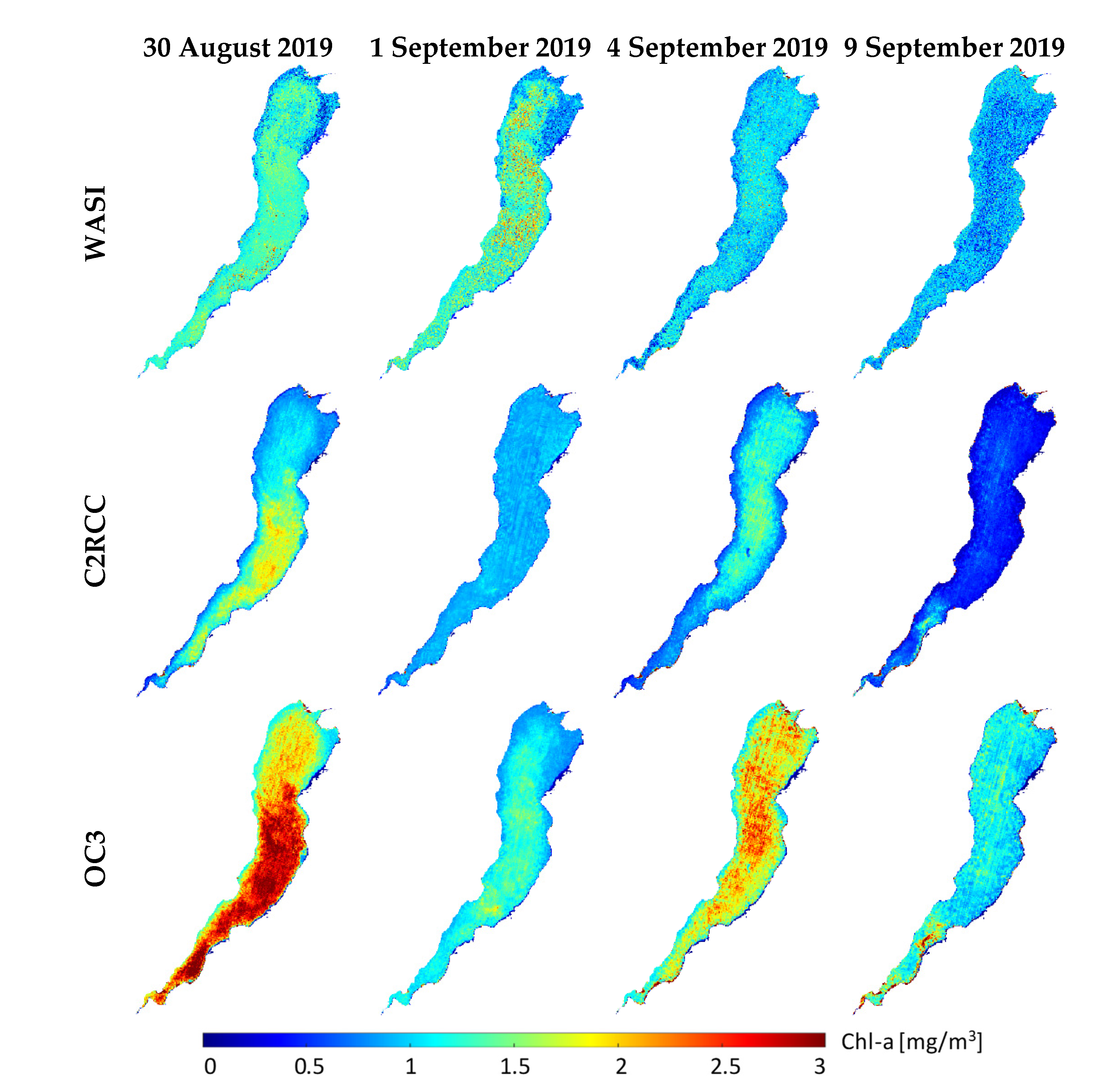C2RCC-E involves a very broad range of IOPs (e.g., $a_{CDOM}$ up to 60 m⁻¹) that may introduce a risk of diverging from the actual solution through the inversion. However, the effect of the range of training IOPs requires more investigations. C2RCC-E showed benefits in the estimation of constituents in Lake Trasimeno. The flexibility of WASI in parametrization allowed for better characterization of the high-CDOM cases in the subalpine lakes and high-Chl-a cases in Lake Trasimeno. In situ matchups of Chl-a reveal the better overall performance of WASI. OC3 captures the overall relative spatiotemporal changes of Chl-a, although the values are mainly overestimated. This problem was noted also in other studies [37,38].

6. Conclusions and Outlooks

This study thoroughly studied the effectiveness of C2RCC, WASI, and OC3 for the estimation of constituents in four Italian lakes representing a relatively wide range of bio-optical conditions. Every method demonstrated its advantages and disadvantages with respect to the others. Therefore, the choice of a suitable method can be assisted by considering some criteria. (i) The first is the complexity of the optical properties of the study area: as demonstrated, WASI provides more flexibility to adapt the inversion to any optical condition. The retrieval of some parameters (e.g., Chl-a in this study) can be problematic based on C2RCC if neither of the two pre-trained networks is representative of the test site. This aspect of C2RCC (i.e., a limited number of pre-defined networks) requires more investigation to better understand its performance in other optically complex conditions. Our results suggest training other networks representative for specific lake water types (e.g., turbid, CDOM-rich, etc.). A globally representative training set (as considered in C2RCC-E) can provide a generic inversion method, although the network type and architecture require more development to provide reliable and robust retrievals. WASI can be applied also in optically shallow waters, which requires the bottom albedo as input, whereas C2RCC and OC3 work only in optically deep waters. Moreover, it should be noted that the coefficients of OC3 are estimated based on samples measured in oceanic and coastal waters [15,60]. Extension of the samples to inland waters may improve the retrievals in inland lakes and rivers. (ii) The size of the water body and the spatial resolution of the imagery affect the computational time: C2RCC is preferable in terms of the computational efficiency, although WASI can be implemented in small lakes with a processing time comparable to that of C2RCC. Moreover, WASI requires more experience and supervision in defining the initial values of the parameters. OC3 also provides a fast means of characterizing the spatiotemporal variations of Chl-a (e.g., anomaly events), although the absolute values might be biased. (iii) The third criteria to consider is the sensor: C2RCC can be applied only to data of pre-defined sensors. Although the C2RCC processor supports most of the important optical satellite data, WASI can be applied on any multi- and hyperspectral dataset acquired from airborne platforms as well as from newly launched and upcoming hyperspectral spaceborne missions such as DESIS, PRISMA, EnMAP, and PACE [20].

References

1. Gurlin, D.; Gitelson, A.A.; Moses, W.J. Remote estimation of chl-a concentration in turbid productive waters—Return to a simple two-band NIR-red model? Remote Sens. Environ. 2011, 115, 3479–3490. [Google Scholar] [CrossRef]
2. Dörnhöfer, K.; Klinger, P.; Heege, T.; Oppelt, N. Multi-sensor satellite and in situ monitoring of phytoplankton development in a eutrophic-mesotrophic lake. Sci. Total Environ. 2018, 612, 1200–1214. [Google Scholar] [CrossRef] [PubMed]
3. Anderson, D.M.; Glibert, P.M.; Burkholder, J.M. Harmful algal blooms and eutrophication: Nutrient sources, composition, and consequences. Estuaries 2002, 25, 704–726. [Google Scholar] [CrossRef]
4. Chislock, M.F.; Doster, E.; Zitomer, R.A.; Wilson, A.E. Eutrophication: Causes, consequences, and controls in aquatic ecosystems. Nat. Educ. Knowl. 2013, 4, 10. [Google Scholar]
5. Kutser, T.; Paavel, B.; Verpoorter, C.; Ligi, M.; Soomets, T.; Toming, K.; Casal, G. Remote Sensing of Black Lakes and Using 810 nm Reflectance Peak for Retrieving Water Quality Parameters of Optically Complex Waters. Remote Sens. 2016, 8, 497. [Google Scholar] [CrossRef]
6. Maeda, E.E.; Lisboa, F.; Kaikkonen, L.; Kallio, K.; Koponen, S.; Brotas, V.; Kuikka, S. Temporal patterns of phytoplankton phenology across high latitude lakes unveiled by long-term time series of satellite data. Remote Sens. Environ. 2019, 221, 609–620. [Google Scholar] [CrossRef]
7. Ansper, A.; Alikas, K. Retrieval of Chlorophyll a from Sentinel-2 MSI Data for the European Union Water Framework Directive Reporting Purposes. Remote Sens. 2018, 11, 64. [Google Scholar] [CrossRef] [Green Version]
8. Niroumand-Jadidi, M.; Bovolo, F.; Bruzzone, L. Novel Spectra-Derived Features for Empirical Retrieval of Water Quality Parameters: Demonstrations for OLI, MSI, and OLCI Sensors. IEEE Trans. Geosci. Remote Sens. 2019, 57, 10285–10300. [Google Scholar] [CrossRef]
9. Lillesand, T.M.; Johnson, W.L.; Deuell, R.L. Use of landsat data to predict the trophic state of Minnesota lakes. Photogramm. Eng. Remote Sens. 1983, 49, 219–229. [Google Scholar]
10. Soomets, T.; Uudeberg, K.; Jakovels, D.; Brauns, A.; Zagars, M.; Kutser, T. Validation and comparison of water quality products in baltic lakes using sentinel-2 msi and sentinel-3 OLCI data. Sensors 2020, 20, 742. [Google Scholar] [CrossRef] [Green Version]
11. Gower, J.; King, S.; Borstad, G.; Brown, L. Detection of intense plankton blooms using the 709 nm band of the MERIS imaging spectrometer. Int. J. Remote Sens. 2005, 26, 2005–2012. [Google Scholar] [CrossRef]
12. Nechad, B.; Ruddick, K.G.; Park, Y. Calibration and validation of a generic multisensor algorithm for mapping of total suspended matter in turbid waters. Remote Sens. Environ. 2010, 114, 854–866. [Google Scholar] [CrossRef]
13. Kutser, T.; Pierson, D.C.; Kallio, K.Y.; Reinart, A.; Sobek, S. Mapping lake CDOM by satellite remote sensing. Remote Sens. Environ. 2005, 94, 535–540. [Google Scholar] [CrossRef]
14. Kutser, T.; Verpoorter, C.; Paavel, B.; Tranvik, L.J. Estimating lake carbon fractions from remote sensing data. Remote Sens. Environ. 2015, 157, 138–146. [Google Scholar] [CrossRef]
15. O’Reilly, J.E.; Werdell, P.J. Chlorophyll algorithms for ocean color sensors—OC4, OC5 & OC6. Remote Sens. Environ. 2019, 229, 32–47. [Google Scholar] [CrossRef]
16. O’Reilly, J.E.; Maritorena, S.; Mitchell, B.G.; Siegel, D.A.; Carder, K.L.; Garver, S.A.; Kahru, M.; McClain, C. Ocean color chlorophyll algorithms for SeaWiFS. J. Geophys. Res. Ocean. 1998, 103, 24937–24953. [Google Scholar] [CrossRef] [Green Version]
17. Brockmann, C.; Doerffer, R.; Peters, M.; Stelzer, K.; Embacher, S.; Ruescas, A. Evolution of the C2RCC neural network for Sentinel 2 and 3 for the retrieval of ocean colour products in normal and extreme optically complex waters. In Proceedings of the ESA Living Planet; ESA: Prague, Czech Republic, 2016. [Google Scholar]
18. Gege, P. WASI-2D: A software tool for regionally optimized analysis of imaging spectrometer data from deep and shallow waters. Comput. Geosci. 2014, 62, 208–215. [Google Scholar] [CrossRef] [Green Version]
19. Niroumand-Jadidi, M.; Bovolo, F.; Bruzzone, L.; Gege, P. Physics-based Bathymetry and Water Quality Retrieval Using PlanetScope Imagery: Impacts of 2020 COVID-19 Lockdown and 2019 Extreme Flood in the Venice Lagoon. Remote Sens. 2020, 12, 2381. [Google Scholar] [CrossRef]
20. Niroumand-Jadidi, M.; Bovolo, F.; Bruzzone, L. Water Quality Retrieval from PRISMA Hyperspectral Images: First Experience in a Turbid Lake and Comparison with Sentinel-2. Remote Sens. 2020, 12, 3984. [Google Scholar] [CrossRef]
21. Arabi, B.; Salama, M.S.; Pitarch, J.; Verhoef, W. Integration of in-situ and multi-sensor satellite observations for long-term water quality monitoring in coastal areas. Remote Sens. Environ. 2020, 239, 111632. [Google Scholar] [CrossRef]
22. Dona, C.; Sanchez, J.M.; Caselles, V.; Dominguez, J.A.; Camacho, A. Empirical relationships for monitoring water quality of lakes and reservoirs through multispectral images. IEEE J. Sel. Top. Appl. Earth Obs. Remote Sens. 2014, 7, 1632–1641. [Google Scholar] [CrossRef]
23. Niroumand-Jadidi, M.; Pahlevan, N.; Vitti, A. Mapping Substrate Types and Compositions in Shallow Streams. Remote Sens. 2019, 11, 262. [Google Scholar] [CrossRef] [Green Version]
24. Xu, M.; Liu, H.; Beck, R.; Lekki, J.; Yang, B.; Shu, S.; Liu, Y.; Benko, T.; Anderson, R.; Tokars, R.; et al. Regionally and Locally Adaptive Models for Retrieving Chlorophyll-a Concentration in Inland Waters from Remotely Sensed Multispectral and Hyperspectral Imagery. IEEE Trans. Geosci. Remote Sens. 2019, 57, 4758–4774. [Google Scholar] [CrossRef]
25. Niroumand-Jadidi, M.; Bovolo, F.; Bruzzone, L. SMART-SDB: Sample-specific multiple band ratio technique for satellite-derived bathymetry. Remote Sens. Environ. 2020, 251, 112091. [Google Scholar] [CrossRef]
26. Niroumand-Jadidi, M.; Vitti, A. Reconstruction of river boundaries at sub-pixel resolution: Estimation and spatial allocation of water fractions. ISPRS Int. J. Geo-Inf. 2017, 6, 383. [Google Scholar] [CrossRef] [Green Version]
27. Niroumand-Jadidi, M.; Vitti, A. Optimal band ratio analysis of WorldView-3 imagery for bathymetry of shallow rivers (case study: Sarca River, Italy). In International Archives of the Photogrammetry, Remote Sensing and Spatial Information Sciences—ISPRS Archives; ISPRS: Prague, Czech Republic, 2016; Volume 41. [Google Scholar]
28. Niroumand-Jadidi, M.; Vitti, A.; Lyzenga, D.R. Multiple Optimal Depth Predictors Analysis (MODPA) for river bathymetry: Findings from spectroradiometry, simulations, and satellite imagery. Remote Sens. Environ. 2018, 218, 132–147. [Google Scholar] [CrossRef]
29. Niroumand-Jadidi, M.; Bovolo, F.; Vitti, A.; Bruzzone, L. A novel approach for bathymetry of shallow rivers based on spectral magnitude and shape predictors using stepwise regression. In Image and Signal Processing for Remote Sensing XXIV; Bruzzone, L., Bovolo, F., Benediktsson, J.A., Eds.; SPIE: Berlin, Germany, 2018; Volume 10789, p. 23. [Google Scholar]
30. Hansen, C.H.; Burian, S.J.; Dennison, P.E.; Williams, G.P. Evaluating historical trends and influences of meteorological and seasonal climate conditions on lake chlorophyll a using remote sensing. Lake Reserv. Manag. 2020, 36, 45–63. [Google Scholar] [CrossRef]
31. Toming, K.; Kutser, T.; Laas, A.; Sepp, M.; Paavel, B.; Nõges, T. First Experiences in Mapping Lake Water Quality Parameters with Sentinel-2 MSI Imagery. Remote Sens. 2016, 8, 640. [Google Scholar] [CrossRef] [Green Version]
32. Hafeez, S.; Wong, M.S.; Abbas, S.; Jiang, G. Assessing the potential of geostationary himawari-8 for mapping surface total suspended solids and its diurnal changes. Remote Sens. 2021, 13, 336. [Google Scholar] [CrossRef]
33. Park, J.E.; Park, K.A. Application of deep learning for speckle removal in goci chlorophyll-a concentration images (2012–2017). Remote Sens. 2021, 13, 585. [Google Scholar] [CrossRef]
34. Kyryliuk, D.; Kratzer, S. Evaluation of Sentinel-3A OLCI Products Derived Using the Case-2 Regional CoastColour Processor over the Baltic Sea. Sensors 2019, 19, 3609. [Google Scholar] [CrossRef] [PubMed] [Green Version]
35. Dörnhöfer, K.; Göritz, A.; Gege, P.; Pflug, B.; Oppelt, N. Water Constituents and Water Depth Retrieval from Sentinel-2A—A First Evaluation in an Oligotrophic Lake. Remote Sens. 2016, 8, 941. [Google Scholar] [CrossRef] [Green Version]
36. Liu, H.; Li, Q.; Shi, T.; Hu, S.; Wu, G.; Zhou, Q. Application of Sentinel 2 MSI Images to Retrieve Suspended Particulate Matter Concentrations in Poyang Lake. Remote Sens. 2017, 9, 761. [Google Scholar] [CrossRef] [Green Version]
37. Freitas, F.H.; Dierssen, H.M. Evaluating the seasonal and decadal performance of red band difference algorithms for chlorophyll in an optically complex estuary with winter and summer blooms. Remote Sens. Environ. 2019, 231, 111228. [Google Scholar] [CrossRef]
38. Le, C.; Hu, C.; Cannizzaro, J.; English, D.; Muller-Karger, F.; Lee, Z. Evaluation of chlorophyll-a remote sensing algorithms for an optically complex estuary. Remote Sens. Environ. 2013, 129, 75–89. [Google Scholar] [CrossRef]
39. Giardino, C.; Brando, V.E.; Dekker, A.G.; Strömbeck, N.; Candiani, G. Assessment of water quality in Lake Garda (Italy) using Hyperion. Remote Sens. Environ. 2007, 109, 183–195. [Google Scholar] [CrossRef]
40. Bresciani, M.; Pinardi, M.; Free, G.; Luciani, G.; Ghebrehiwot, S.; Laanen, M.; Peters, S.; Della Bella, V.; Padula, R.; Giardino, C. The Use of Multisource Optical Sensors to Study Phytoplankton Spatio-Temporal Variation in a Shallow Turbid Lake. Water 2020, 12, 284. [Google Scholar] [CrossRef] [Green Version]
41. Free, G.; Bresciani, M.; Pinardi, M.; Ghirardi, N.; Luciani, G.; Caroni, R.; Giardino, C. A regional evaluation of the influence of climate change on long term trends in chlorophyll-a in large Italian lakes from satellite data. Earth Syst. Dyn. 2020, 1–19. [Google Scholar] [CrossRef]
42. GLaSS. WP5 Innovation and Application through Use Cases D.5.3 Use Case 2: Deep Clear Lakes with Increasing Eutrophication; CNR: Milan, Italy, 2015. [Google Scholar]
43. Giardino, C.; Bresciani, M.; Valentini, E.; Gasperini, L.; Bolpagni, R.; Brando, V.E. Airborne hyperspectral data to assess suspended particulate matter and aquatic vegetation in a shallow and turbid lake. Remote Sens. Environ. 2015, 157, 48–57. [Google Scholar] [CrossRef]
44. Bresciani, M.; Cazzaniga, I.; Austoni, M.; Sforzi, T.; Buzzi, F.; Morabito, G.; Giardino, C. Mapping phytoplankton blooms in deep subalpine lakes from Sentinel-2A and Landsat-8. Hydrobiologia 2018, 824, 197–214. [Google Scholar] [CrossRef] [Green Version]
45. Cerasino, L.; Salmaso, N. Diversity and distribution of cyanobacterial toxins in the Italian subalpine lacustrine district. Oceanol. Hydrobiol. Stud. 2012, 41, 54–63. [Google Scholar] [CrossRef]
46. Pereira-Sandoval, M.; Ruescas, A.; Urrego, P.; Ruiz-Verdú, A.; Delegido, J.; Tenjo, C.; Soria-Perpinyà, X.; Vicente, E.; Soria, J.; Moreno, J. Evaluation of Atmospheric Correction Algorithms over Spanish Inland Waters for Sentinel-2 Multi Spectral Imagery Data. Remote Sens. 2019, 11, 1469. [Google Scholar] [CrossRef] [Green Version]
47. Warren, M.A.; Simis, S.G.H.; Martinez-Vicente, V.; Poser, K.; Bresciani, M.; Alikas, K.; Spyrakos, E.; Giardino, C.; Ansper, A. Assessment of atmospheric correction algorithms for the Sentinel-2A MultiSpectral Imager over coastal and inland waters. Remote Sens. Environ. 2019, 225, 267–289. [Google Scholar] [CrossRef]
48. Ritchie, J.C.; Zimba, P.V.; Everitt, J.H. Remote Sensing Techniques to Assess Water Quality. Photogramm. Eng. Remote Sens. 2003, 69, 695–704. [Google Scholar] [CrossRef] [Green Version]
49. Seegers, B.N.; Stumpf, R.P.; Schaeffer, B.A.; Loftin, K.A.; Werdell, P.J. Performance metrics for the assessment of satellite data products: An ocean color case study. Opt. Express 2018, 26, 7404. [Google Scholar] [CrossRef] [PubMed] [Green Version]
50. APHA. Standard Methods for the Examination of Water and Wastewater; American Public Health Association: Washington, DC, USA, 1985. [Google Scholar]
51. APAT. Metodi Analitici Per Le Acque. Available online: https://www.isprambiente.gov.it/it/pubblicazioni/manuali-e-linee-guida/metodi-analitici-per-le-acque (accessed on 4 November 2020).
52. Dekker, A.G.; Phinn, S.R.; Anstee, J.; Bissett, P.; Brando, V.E.; Casey, B.; Fearns, P.; Hedley, J.; Klonowski, W.; Lee, Z.P.; et al. Intercomparison of shallow water bathymetry, hydro-optics, and benthos mapping techniques in Australian and Caribbean coastal environments. Limnol. Oceanogr. Methods 2011, 9, 396–425. [Google Scholar] [CrossRef] [Green Version]
53. Giardino, C.; Candiani, G.; Bresciani, M.; Lee, Z.; Gagliano, S.; Pepe, M. BOMBER: A tool for estimating water quality and bottom properties from remote sensing images. Comput. Geosci. 2012, 45, 313–318. [Google Scholar] [CrossRef]
54. Doerffer, R.; Schiller, H. The MERIS Case 2 water algorithm. Int. J. Remote Sens. 2007, 28, 517–535. [Google Scholar] [CrossRef]
55. SNAP Entinel Application Platform (SNAP). Available online: step.esa.int/main/download/snap-download (accessed on 10 June 2021).
56. Gege, P. The water color simulator WASI: An integrating software tool for analysis and simulation of optical in situ spectra. Comput. Geosci. 2004, 30, 523–532. [Google Scholar] [CrossRef]
57. Gege, P. WASI (Water Colour Simulator). Available online: www.ioccg.org/data/software.html (accessed on 10 June 2021).
58. Gege, P.; Albert, A. A Tool for Inverse Modeling of Spectral Measurements in Deep and Shallow Waters. In Remote Sensing of Aquatic Coastal Ecosystem Processes; Richardson, L.L., LeDrew, E.F., Eds.; Springer Netherlands: Dordrecht, The Netherlands, 2006; pp. 81–109. ISBN 978-1-4020-3968-3. [Google Scholar]
59. Gege, P. Chapter 2—Radiative Transfer Theory for Inland Waters. In Bio-Optical Modeling and Remote Sensing of Inland Waters; Mishra, D.R., Ogashawara, I., Gitelson, A.A., Eds.; Elsevier: Amsterdam, The Netherlands, 2017; pp. 25–67. ISBN 978-0-12-804644-9. [Google Scholar]
60. Valente, A.; Sathyendranath, S.; Brotas, V.; Groom, S.; Grant, M.; Taberner, M.; Antoine, D.; Arnone, R.; Balch, W.M.; Barker, K.; et al. A compilation of global bio-optical in situ data for ocean-colour satellite applications. Earth Syst. Sci. Data 2016, 8, 235–252. [Google Scholar] [CrossRef] [Green Version]
61. Soja-Woźniak, M.; Darecki, M.; Wojtasiewicz, B.; Bradtke, K. Laboratory measurements of remote sensing reflectance of selected phytoplankton species from the Baltic Sea. Oceanologia 2018, 60, 86–96. [Google Scholar] [CrossRef]
Figure 1. The studied lakes (a) Garda, (b) Ledro, (c) Idro, and (d) Trasimeno illustrated on Sentinel-2 images. The measurement stations are shown by yellow symbols.
Remotesensing 13 02381 g001
Figure 2. Remote sensing reflectance (Rrs) derived from C2RCC for the studied lakes.
Remotesensing 13 02381 g002
Figure 3. Temporal variation of (a) average Chl-a and (b) its RSTD derived from different methods in Lake Garda. C2RCC-NE is the combined results of C2RCC-N (low-CDOM) and C2RCC-E (high-CDOM).
Remotesensing 13 02381 g003
Figure 4. Temporal variation of (a) TSM and (b) CDOM derived from different methods in Lake Garda.
Remotesensing 13 02381 g004
Figure 5. Temporal variation of Chl-a derived from different methods at the measurement station in Lake Garda.
Remotesensing 13 02381 g005
Figure 6. Matchup validation of Chl-a for (a) C2RCC-NE, (b) WASI, and (c) OC3 methods at the measurement station in Lake Garda. The dashed lines are the 1:1 lines, and the solid lines are the regression lines. Samples associated with Sentinel-2A and Sentinel-2B are shown by green and blue colors, respectively.
Remotesensing 13 02381 g006
Figure 7. Chl-a maps derived from different methods for a high-CDOM case (24 October 2018).
Remotesensing 13 02381 g007
Figure 8. Multitemporal Chl-a maps derived from different methods for low-CDOM cases.
Remotesensing 13 02381 g008
Figure 9. Multitemporal TSM maps derived from different methods for low-CDOM cases.
Remotesensing 13 02381 g009
Figure 10. Multitemporal CDOM maps derived from different methods for low-CDOM cases.
Remotesensing 13 02381 g010
Figure 11. Temporal profile of the average Chl-a derived from different methods in Lake Ledro.
Remotesensing 13 02381 g011
Figure 12. Matchup validation of Chl-a for (a) C2RCC, (b) WASI, and (c) OC3 methods at the measurement station in Lake Ledro. The dashed lines are the 1:1 lines, and the solid lines are the regression lines.
Remotesensing 13 02381 g012
Figure 13. Multitemporal Chl-a maps derived from different methods in Lake Ledro.
Remotesensing 13 02381 g013
Figure 14. Temporal profile of the average Chl-a derived from different methods in Lake Idro.
Remotesensing 13 02381 g014
Figure 15. Matchup validation of Chl-a for (a) C2RCC, (b) WASI, and (c) OC3 methods at the measurement station in Lake Idro. The dashed lines are the 1:1 lines, and the solid lines are the regression lines.
Remotesensing 13 02381 g015
Figure 16. Multitemporal Chl-a maps derived from different methods in Lake Idro.
Remotesensing 13 02381 g016
Figure 17. Temporal profile of the average Chl-a derived from different methods in Lake Trasimeno.
Remotesensing 13 02381 g017
Figure 18. Multitemporal Chl-a maps derived from different methods in Lake Trasimeno.
Remotesensing 13 02381 g018
Figure 19. Matchup validation of Chl-a derived from (a) C2RCC-E, (b) WASI, and (c) OC3 at the two measurement stations in Lake Trasimeno. The dashed lines are the 1:1 lines, and the solid lines are the regression lines. Samples associated with Sentinel-2A and Sentinel-2B are shown by green and blue colors, respectively.
Remotesensing 13 02381 g019