
Integrating Geophysical and Photographic Data to Visualize the Quarried Structures of the Roman Town of Bassianae

 ,
, 
 , , , ,
Abstract
:1. Introduction
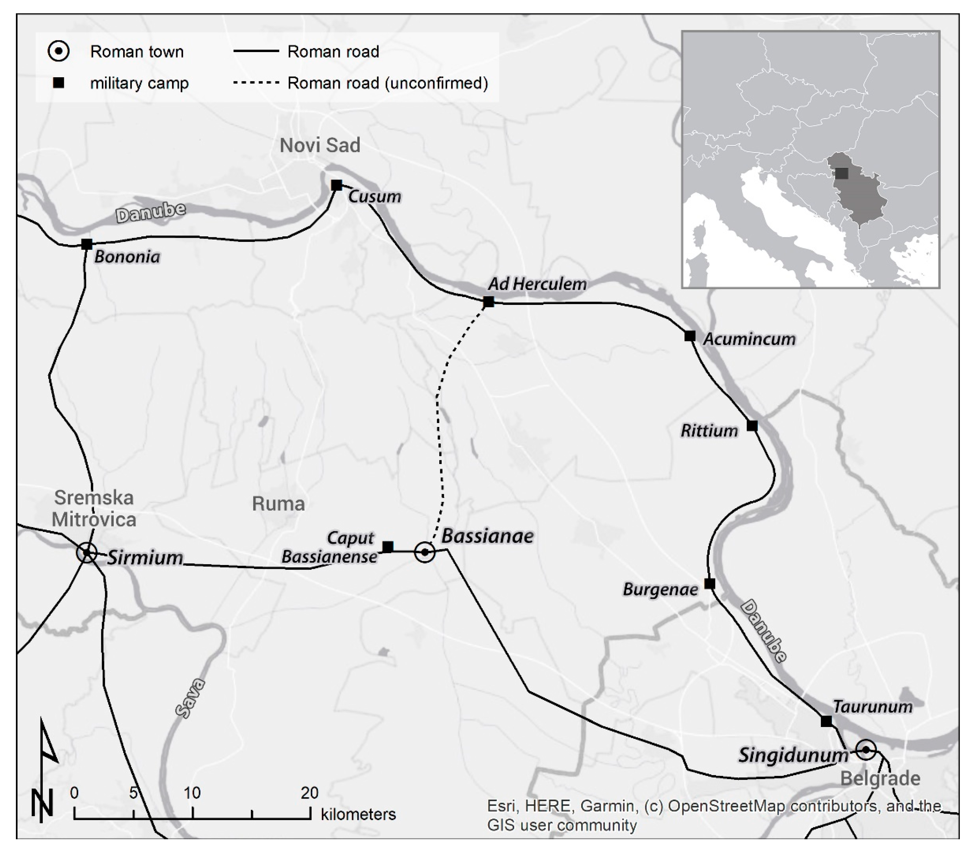
1.1. Bassianae’s History
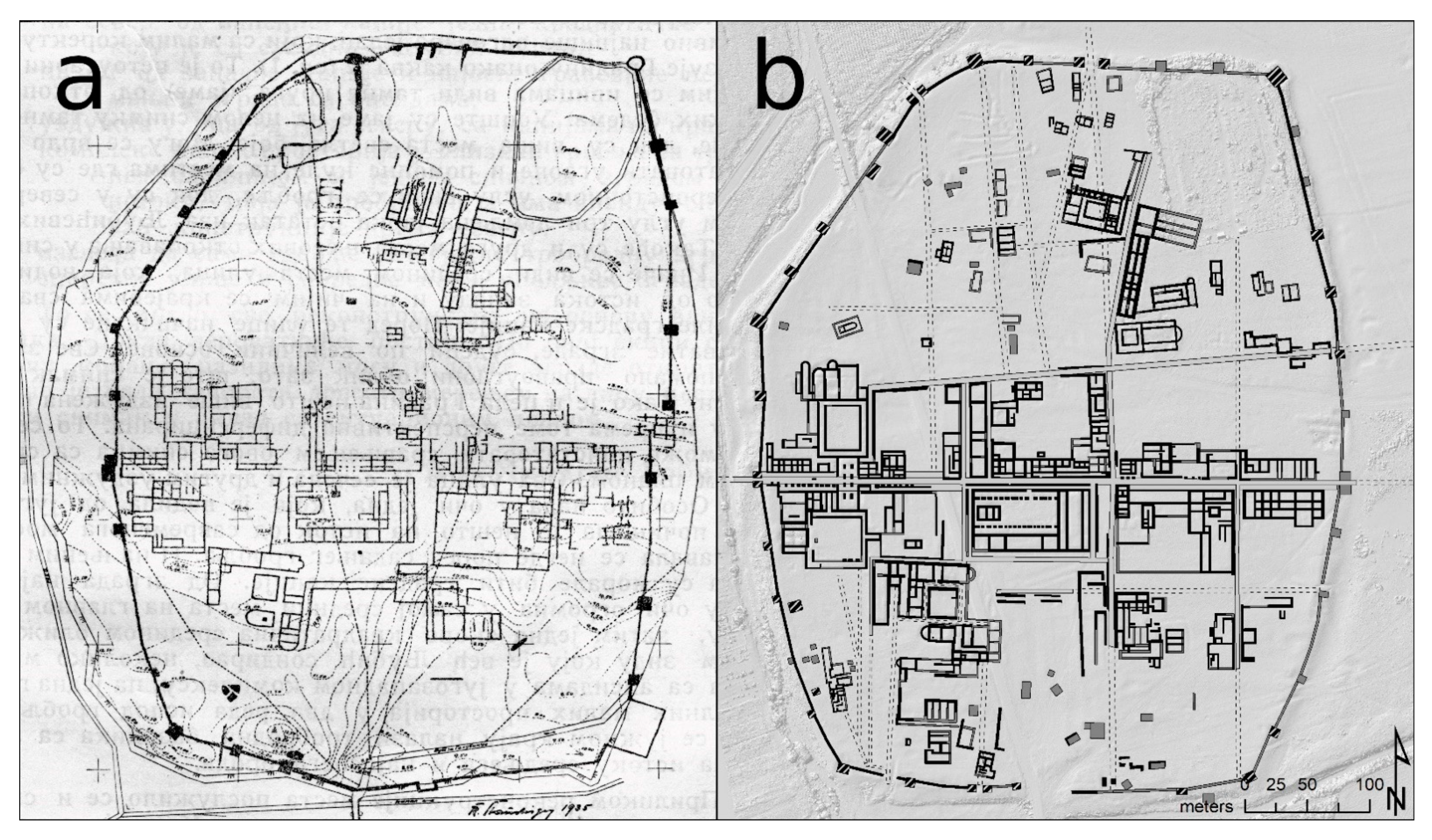
1.2. Research History
1.3. New Goals and Research Questions
2. Materials and Methods
2.1. Geophysical Prospection
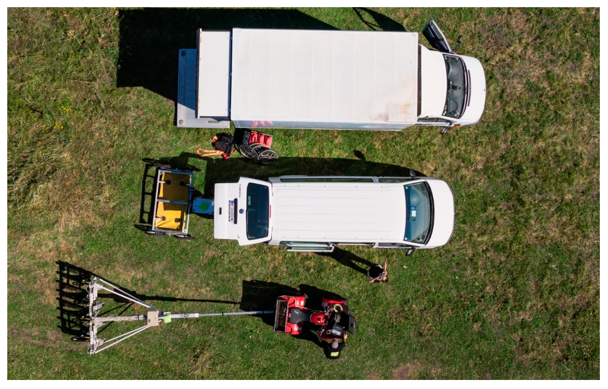
2.1.1. Data Acquisition
2.1.2. Data Processing
2.2. Airborne Imaging
2.2.1. Data Acquisition
2.2.2. Data Processing
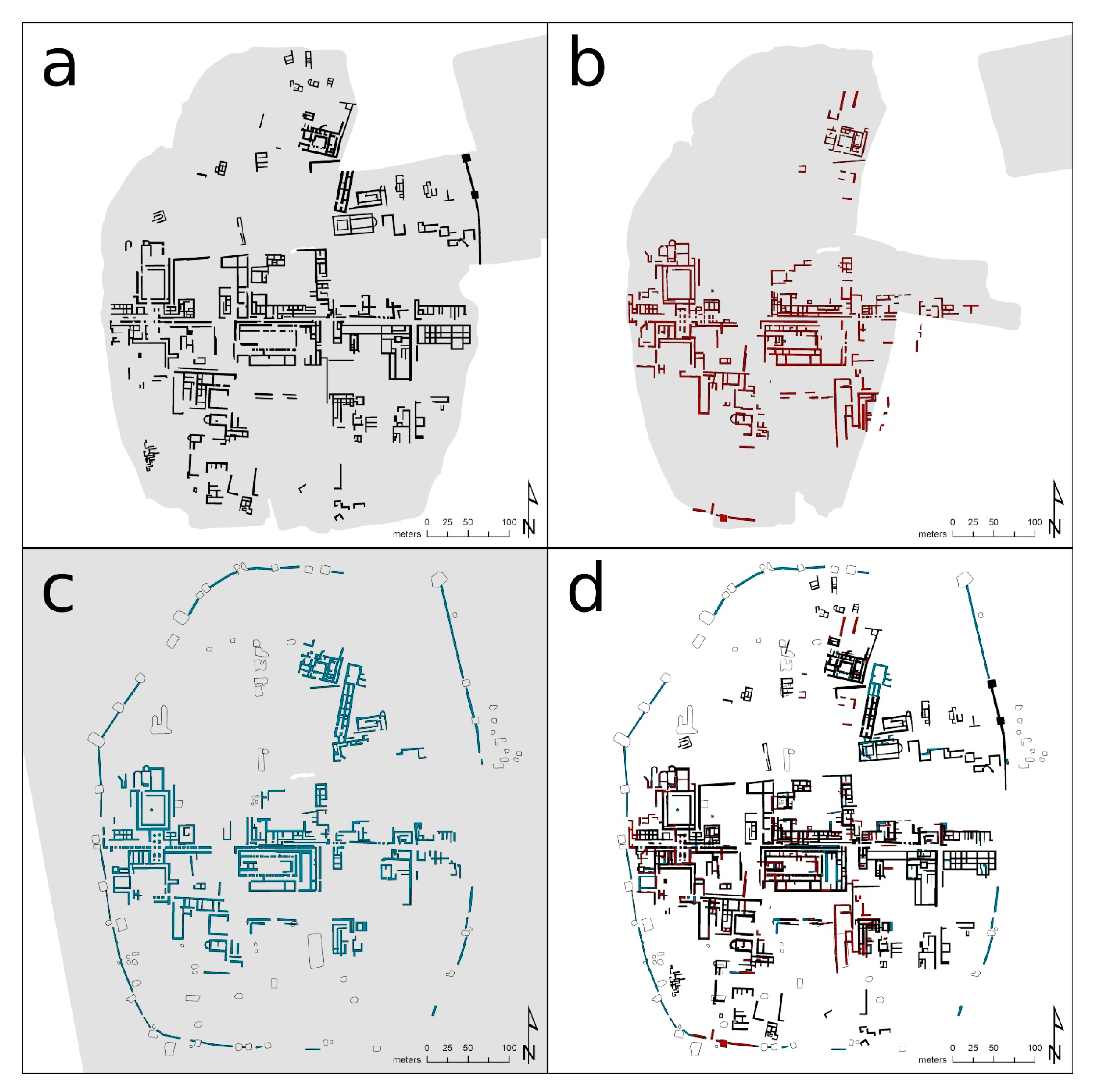
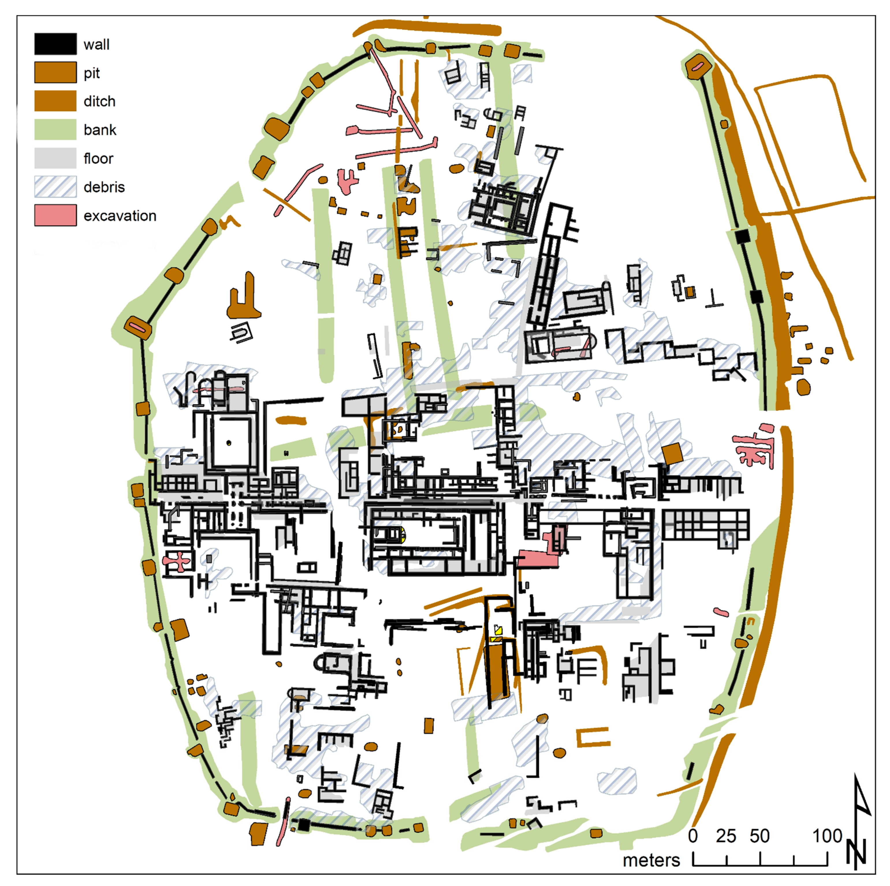
3. Results
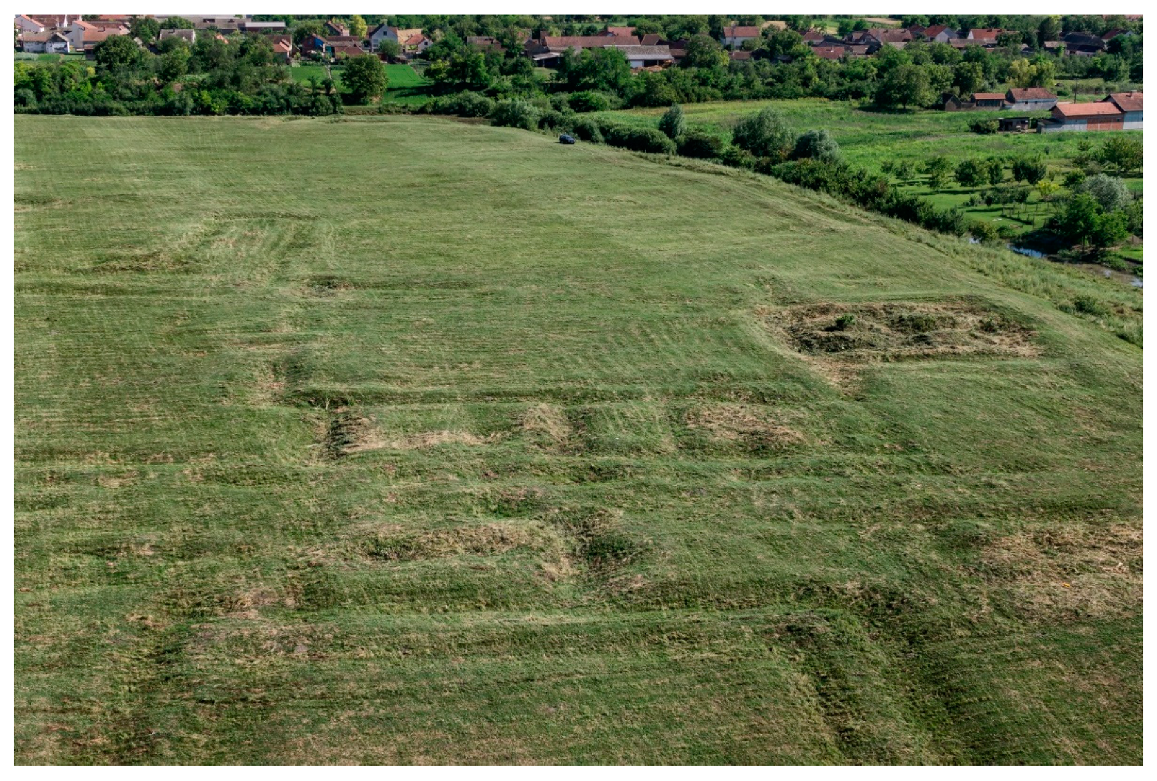
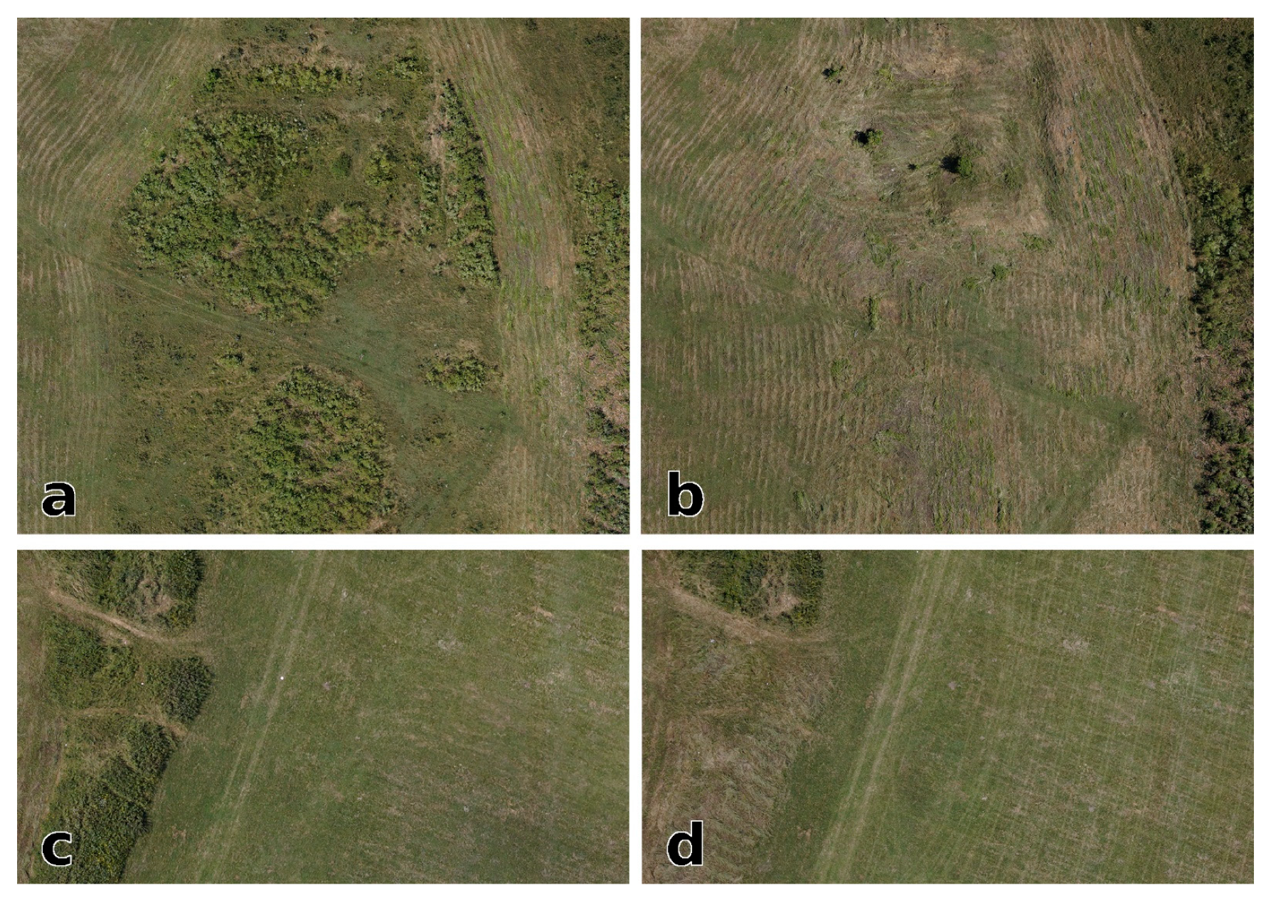
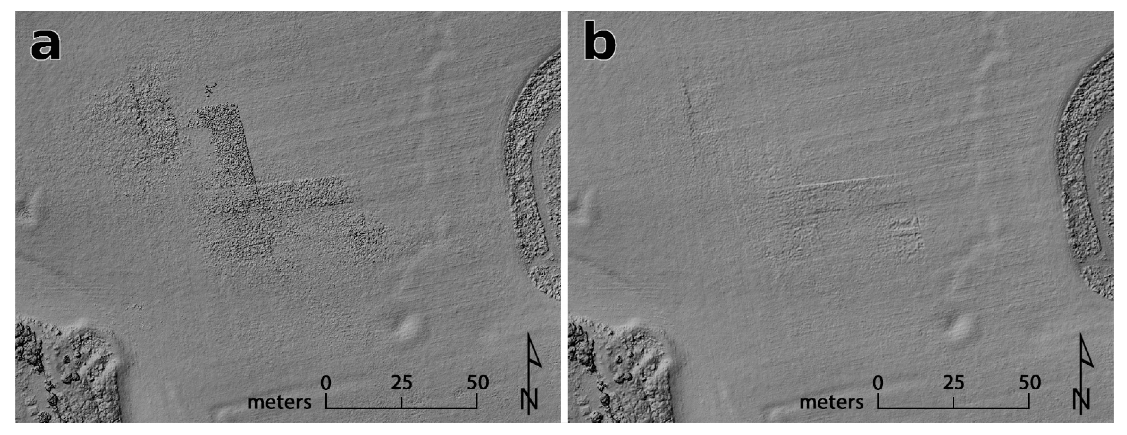
3.1. Digital Surface Model
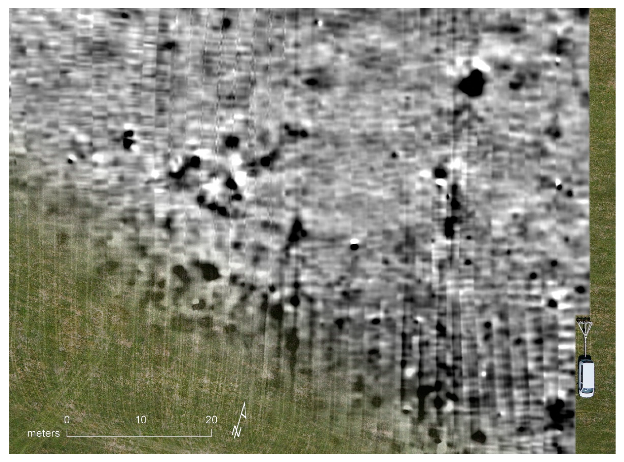
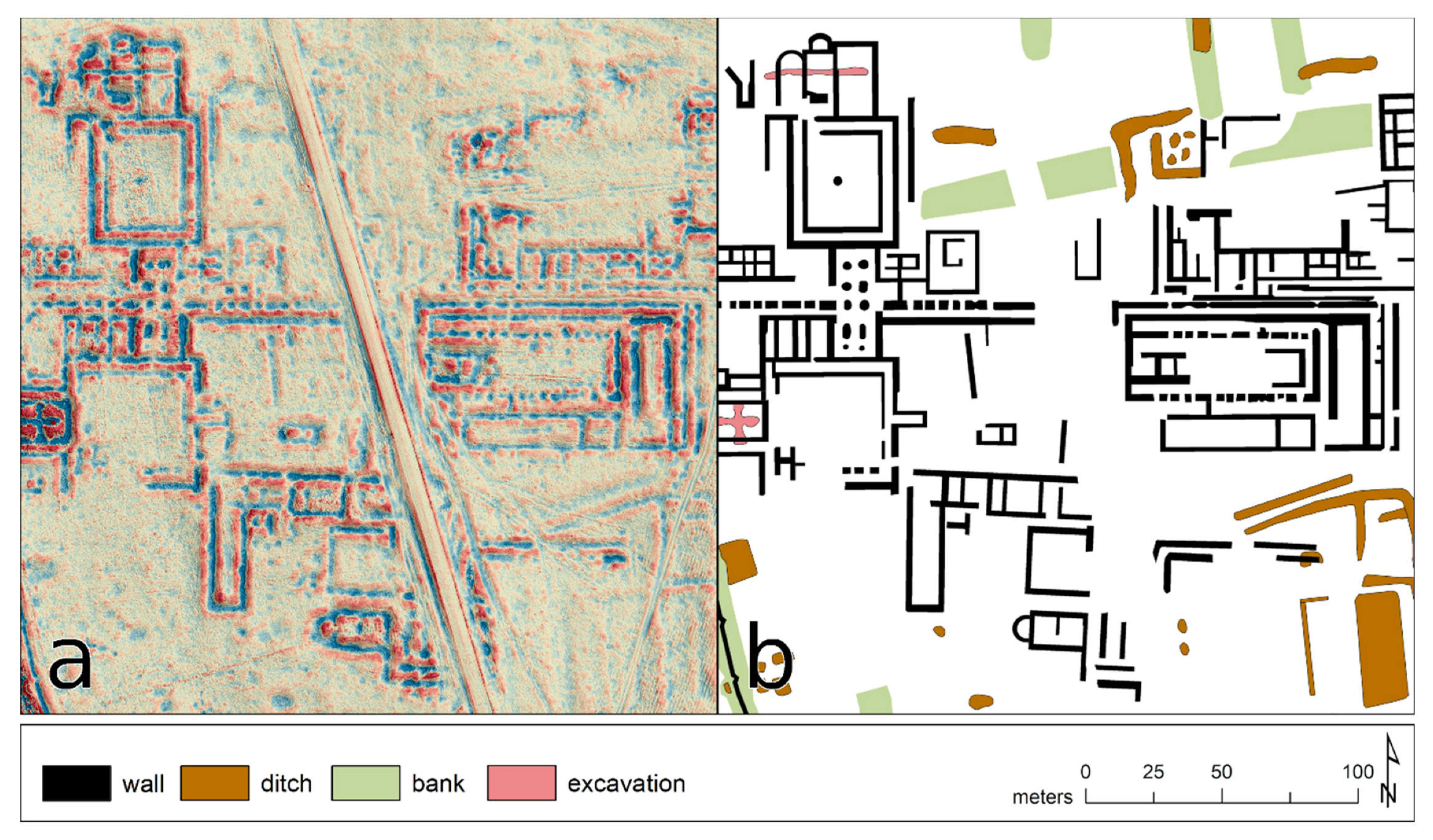
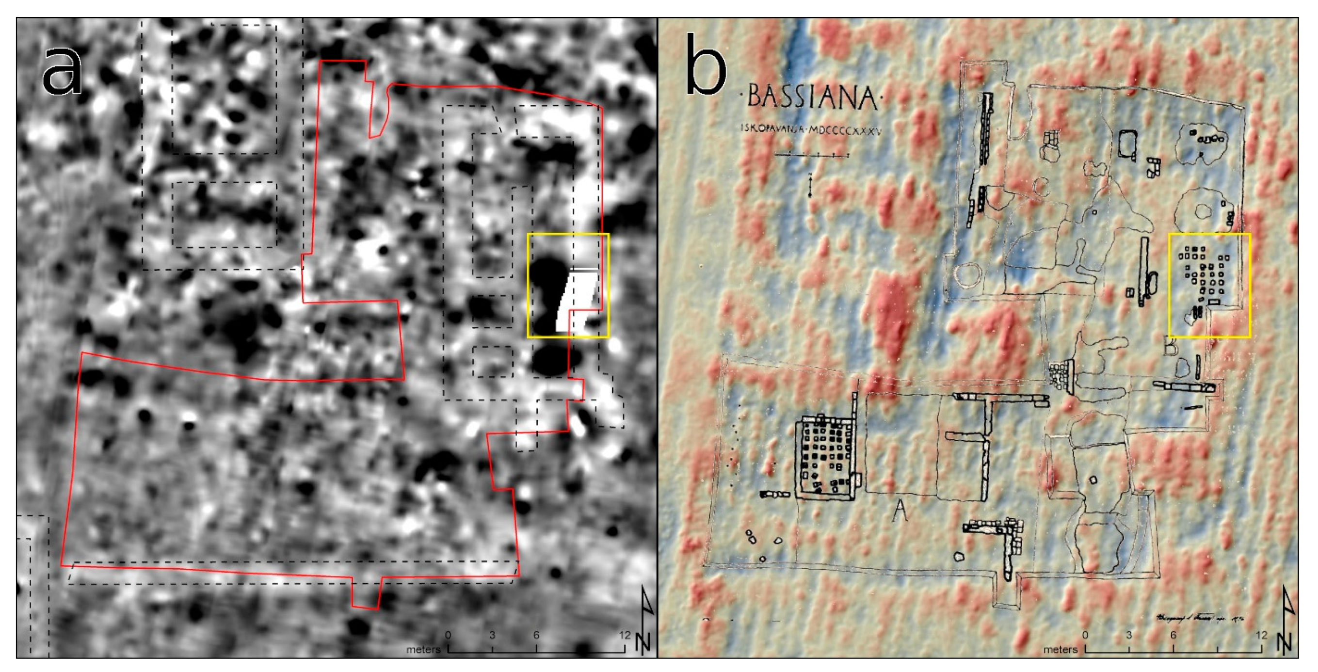
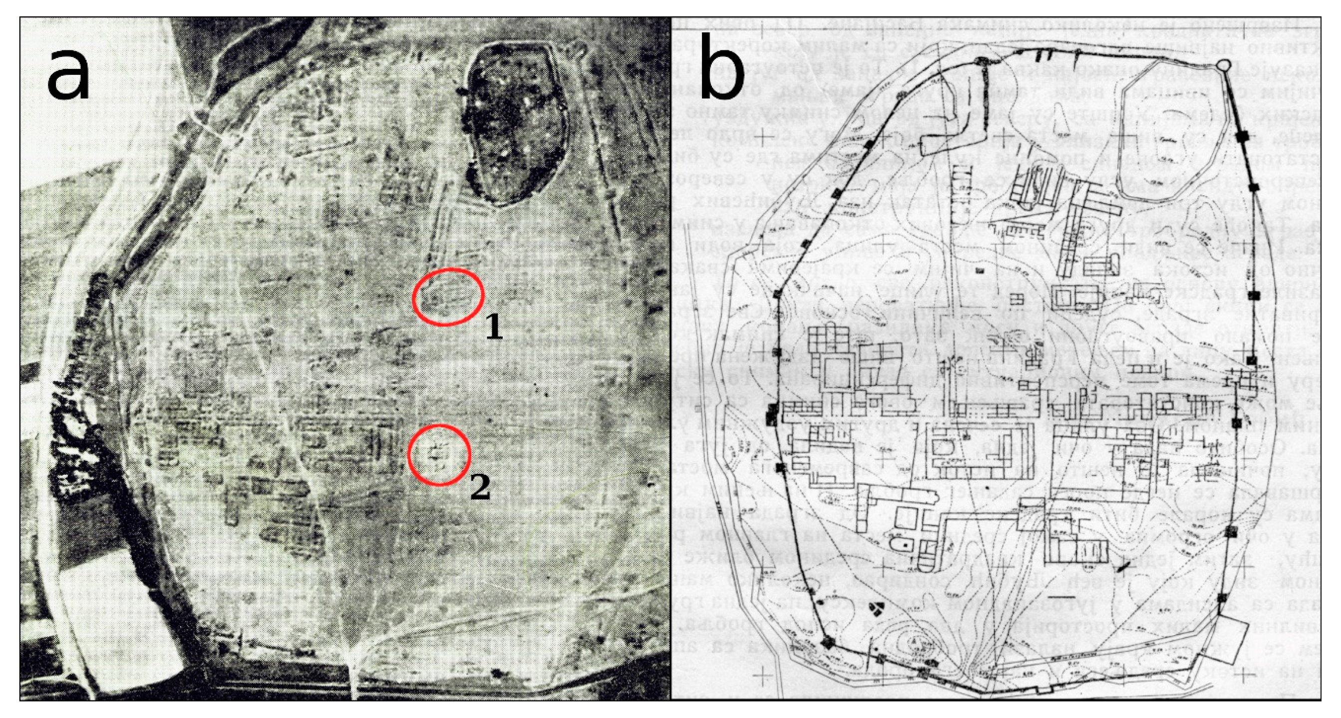
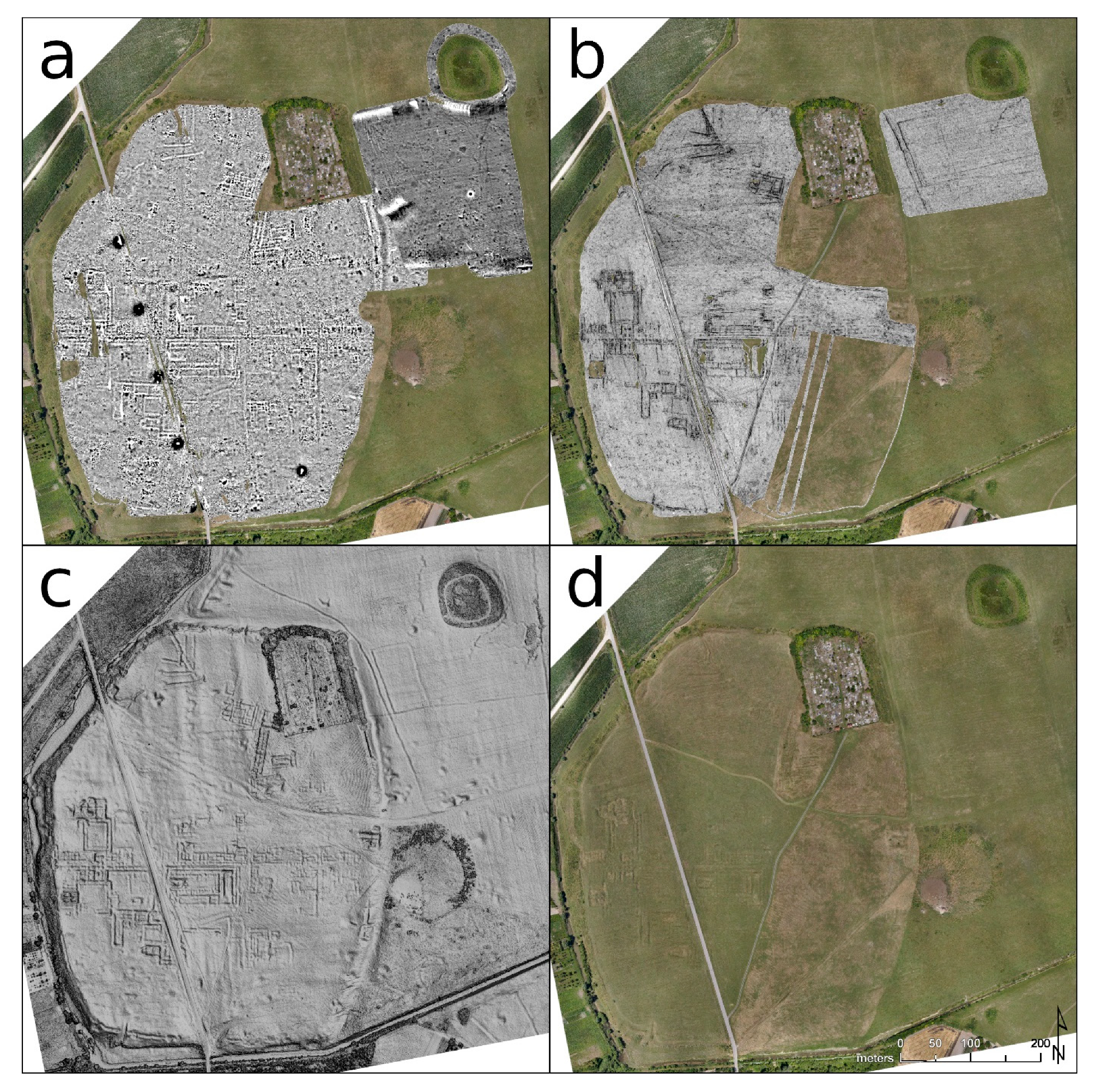
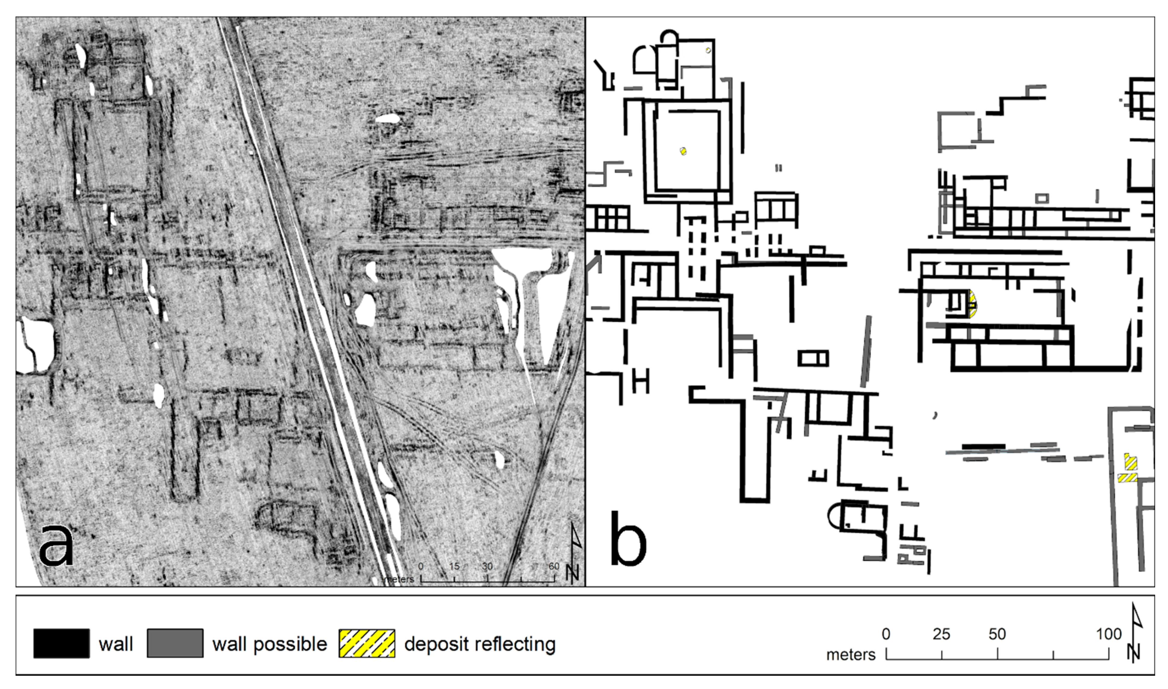
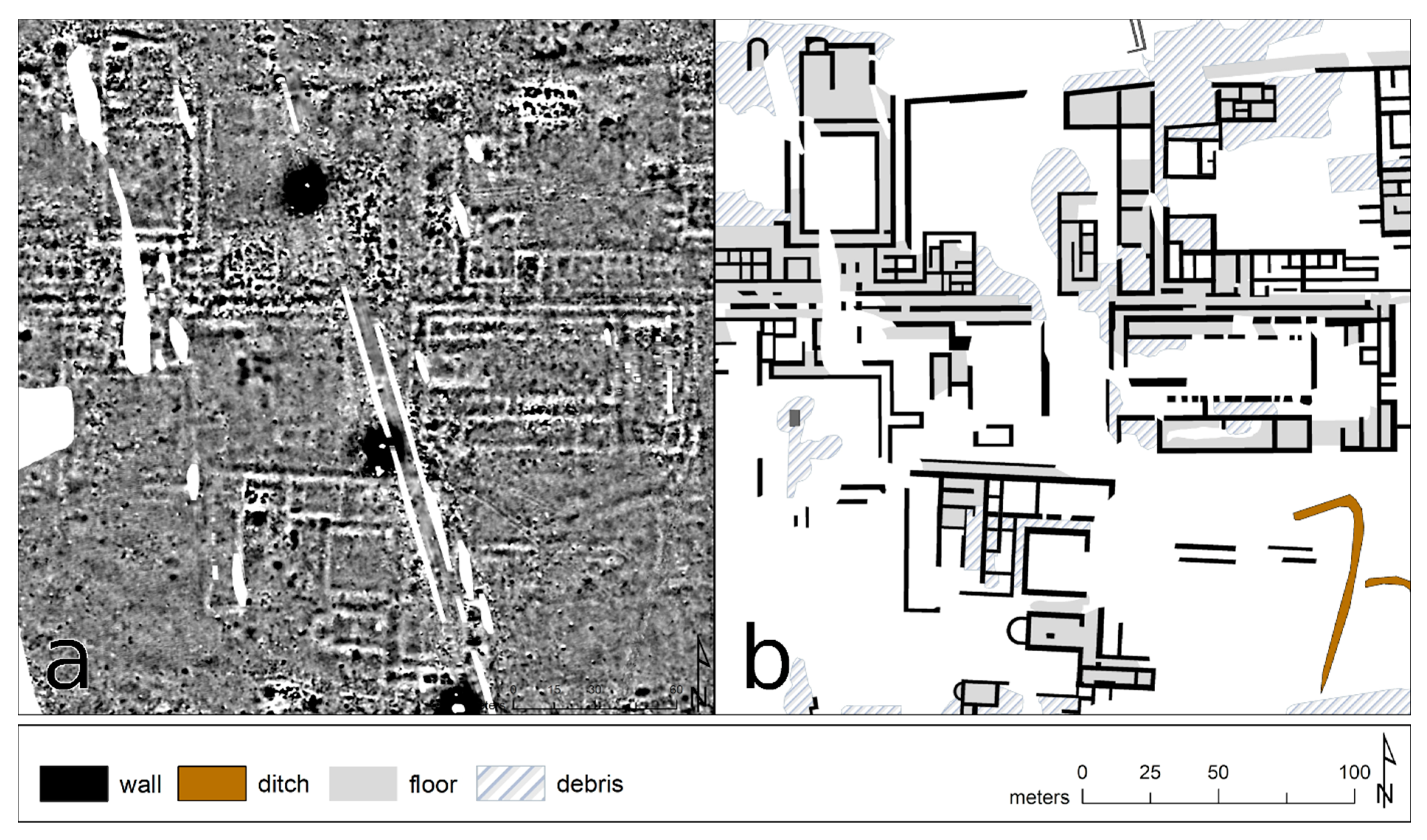
3.2. Ground-Penetrating Radar
3.3. Magnetometry
4. Discussion
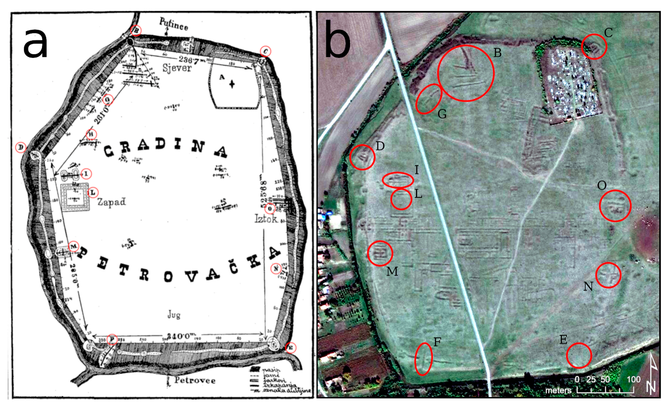
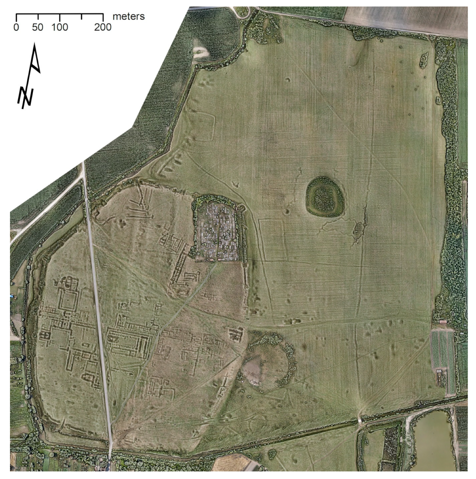
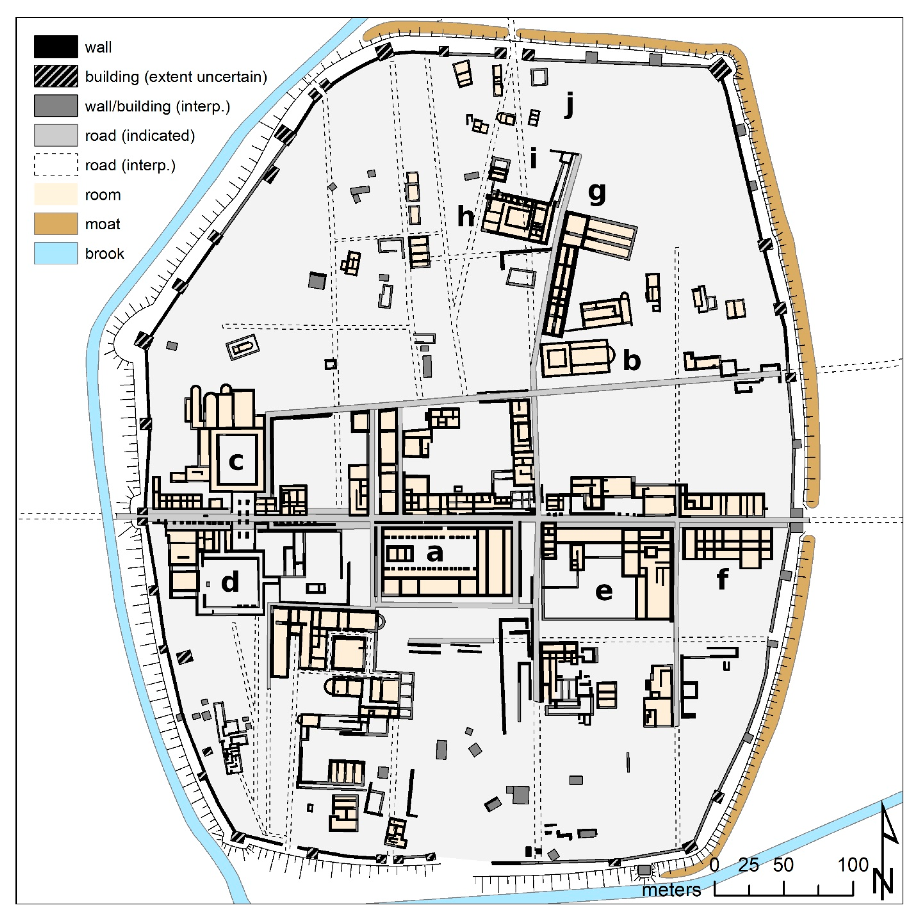
4.1. Fortification
4.2. Road Network and Insulae
4.3. Outer Area
4.4. Round-Up
5. Conclusions
Author Contributions
Funding
Acknowledgments
Conflicts of Interest
References
- Beutler, F. Ein neuer Decurio von Bassianae. In “Eine ganz normale Inschrift” … und ähnliches zum Geburtstag von Ekkehard Weber—Festschrift zum 30. April 2005; Beutler, F., Hameter, W., Eds.; Österreichische Gesellschaft für Archäologie: Wien, Austria, 2005; pp. 215–216. [Google Scholar]
- Milin, M. Bassianae. In The Autonomous Towns of Noricum and Pannonia. Pannonia II; Šašel Kos, M., Scherrer, P., Eds.; Narodni muzej Slovenije: Ljubljana, Slovenia, 2004; pp. 253–268. ISBN 961-6169-30-0. [Google Scholar]
- Dušanić, S. Bassianae and Its Territory. Archaeol. Iugosl. 1967, 8, 67–81. [Google Scholar]
- Notitia Dignitatum, Accedunt Notitia Urbis Constantinopolitanae et Latercula Provinciarum; Seeck, O. (Ed.) Minerva: Frankfurt am Main, Germany, 1962. [Google Scholar]
- Ljubić, Š. Arkeologička izkapanja na Petrovačkoj gradini u Sriemu, gdje tobož starorimska Bassianis. Viestn. Hrvat. Arkeol. Družtva 1883, 5, 33–49. [Google Scholar]
- Grbić, M. Arhitektura u Basijani (Sremski Petrovci) II. Glas. Istor. Društva Novom Sadu 1937, 10, 1–7. [Google Scholar]
- Grbić, M. Bassianae, Yugoslavia (Plate VI). Antiquity 1936, 10, 475–477. [Google Scholar] [CrossRef]
- Grbić, M. Arhitektura u Basijani (Sremski Petrovci) I. Glas. Istor. Društva Novom Sadu 1936, 9, 19–31. [Google Scholar]
- Crawford, O.G.S. Air Survey and Archaeology. Geogr. J. 1923, 61, 342–360. [Google Scholar] [CrossRef]
- Reeves, D.M. Aerial Photography and Archaeology. Am. Antiq. 1936, 2, 102–107. [Google Scholar] [CrossRef]
- Bugarski, I.; Ivanišević, V. Primena aerofotografije u srpskoj arheologiji. Saopštenja 2014, 46, 251–263. [Google Scholar]
- Crawford, O.G.S. Letter of O.G.S. Crawford to Miodrag Grbić; Archive of the Serbian Academy of Sciences and Arts: Sremski Karlovci, Serbia, 13 October 1936. [Google Scholar]
- Bandović, A.D. Miodrag Grbić I Nastanak Kulturno-Istorijske Arheologije U Srbiji. Ph.D. Thesis, University of Belgrade, Belgrade, Serbia, 2019. [Google Scholar]
- Keay, S.; Millett, M.; Poppy, S.; Robinson, J.; Taylor, J.; Terrenato, N. Falerii Novi: A new survey of the walled area. Pap. Br. Sch. Rome 2000, 68, 1–93. [Google Scholar] [CrossRef]
- Eder-Hinterleitner, A.; Ertel, C.; Ferschin, P.; Kandler, M.; Löcker, K.; Melichar, P.; Neubauer, W.; Seren, S. Das Forum des municipium Aelium Karnuntum. In Legionsadler Und Druidenstab: Vom Legionslager Zur Donaumetropole; Katalogband; Sonderausstellung Aus Anlass Des Jubiläums “2000 Jahre Carnuntum”, Archäologisches Museum Carnuntinum Bad Deutsch-Altenburg 21 März 2006–11 November 2007; Humer, F., Ed.; Amt der NÖ Landesregierung: St. Pölten, Austria, 2006; pp. 280–295. ISBN 9783854602293. [Google Scholar]
- Keay, S.; Earl, G.P.; Hay, S.; Kay, S.; Ogden, J.; Strutt, K.D. The role of integrated geophysical survey methods in the assessment of archaeological landscapes: The case of Portus. Archaeol. Prospect. 2009, 16, 154–166. [Google Scholar] [CrossRef]
- Seren, S.; Hinterleitner, A.; Gschwind, M.; Neubauer, W.; Löcker, K. Combining data of different GPR systems of surveys of the roman fort Qreiye-cAyyash, Syria. Archeosciences 2009, 33, 353–355. [Google Scholar] [CrossRef] [Green Version]
- Saey, T.; Van Meirvenne, M.; de Smedt, P.; Neubauer, W.; Trinks, I.; Verhoeven, G.J.J.; Seren, S. Integrating multi-receiver electromagnetic induction measurements into the interpretation of the soil landscape around the school of gladiators at Carnuntum. Eur. J. Soil Sci. 2013, 64, 716–727. [Google Scholar] [CrossRef]
- Gugl, C.; Neubauer, W.; Nau, E.; Jernej, R. Das Militärlager in Virunum (Noricum): Zur Stationierung von römischen Truppen (singulares) an Statthaltersitzen-Teil 2. CarnuntumJB 2016, 2014, 55–66. [Google Scholar] [CrossRef]
- Keay, S.J.; Parcak, S.H.; Strutt, K.D. High resolution space and ground-based remote sensing and implications for landscape archaeology: The case from Portus, Italy. JAS 2014, 52, 277–292. [Google Scholar] [CrossRef]
- Neubauer, W.; Gugl, C.; Scholz, M.; Verhoeven, G.J.J.; Trinks, I.; Löcker, K.; Doneus, M.; Saey, T.; Van Meirvenne, M. The discovery of the school of gladiators at Carnuntum, Austria. Antiquity 2014, 88, 173–190. [Google Scholar] [CrossRef] [Green Version]
- Gugl, C.; Neubauer, W.; Nau, E.; Jernej, R. New evidence for a Roman military camp at Virunum (Noricum). Archaeol. Pol. 2015, 53, 289–292. [Google Scholar]
- Gugl, C.; Neubauer, W.; Wallner, M.; Löcker, K.; Verhoeven, G.J.J.; Humer, F. Die Canabae von Carnuntum. Erste Ergebnisse der geophysikalischen Messungen 2012–2015. In Legionslager und Canabae Legionis in Pannonien: Internationale Archäologische Konferenz. Budapest, 16–17 November 2015; Beszédes, J., Ed.; Historisches Museum der Stadt Budapest: Budapest, Hungary, 2016; pp. 29–43. ISBN 978-615-5341-31-1. [Google Scholar]
- Lambers, L.; Fassbinder, J.; Ritter, S.; Ben Tahar, S. Meninx-Geophysical prospection of a Roman town in Jerba, Tunisia. In AP2017: 12th International Conference of Archaeological Prospection, University of Bradford, Bradford, UK, 12–16 September 2017; Jennings, B., Gaffney, C.F., Sparrow, T., Gaffney, S., Eds.; Archaeopress Publishing: Oxford, UK, 2017; pp. 135–137. ISBN 9781784916787. [Google Scholar]
- Neubauer, W.; Wallner, M.; Gugl, C.; Löcker, K.; Vonkilch, A.; Trausmuth, T.; Nau, E.; Jansa, V.; Wilding, J.; Hinterleitner, A.; et al. Zerstörungsfreie archäologische Prospektion des römischen Carnuntum—erste Ergebnisse des Forschungsprojekts “ArchPro Carnuntum”. In Carnuntum Jahrbuch 2017; Pülz, A., Ed.; Verlag der Österreichischen Akademie der Wissenschaften: Wien, Austria, 2018; pp. 55–75. ISBN 978-3-7001-8372-3. [Google Scholar]
- Ritter, S.; Ben Tahar, S.; Fassbinder, J.W.E.; Lambers, L. Landscape archaeology and urbanism at Meninx: Results of geophysical prospection on Jerba (2015). J. Rom. Archaeol. 2018, 31, 357–372. [Google Scholar] [CrossRef] [Green Version]
- Pasquinucci, M.; Ducci, S.; Menchelli, S.; Ribolini, A.; Bianchi, A.; Bini, M.; Sartini, S. Ground Penetrating Radar Survey of Urban Sites in North Coastal Etruria: Pisae, Portus Pisanus, Vada Volaterrana. In Urban Landscape Survey in Italy and the Mediterranean; Vermeulen, F., Burgers, G.-J., Keay, S.J., Corsi, C., Eds.; Oxbow Books: Oxford, UK, 2012; pp. 149–159. ISBN 978-1-84217-486-9. [Google Scholar]
- The Isola Sacra Survey: Ostia, Portus and the Port System of Imperial Rome; Keay, S.; Millett, M.; Strutt, K.; Germoni, P. (Eds.) McDonald Institute for Archaeological Research, University of Cambridge: Cambridge, UK, 2020; ISBN 978-1-902937-94-6. [Google Scholar]
- Pisz, M.; Tomas, A.; Hegyi, A. Non-destructive research in the surroundings of the Roman Fort Tibiscum (today Romania). Archaeol. Prospect. 2020, 27, 219–238. [Google Scholar] [CrossRef] [Green Version]
- Verdonck, L.; Launaro, A.; Vermeulen, F.; Millett, M. Ground-penetrating radar survey at Falerii Novi: A new approach to the study of Roman cities. Antiquity 2020, 94, 705–723. [Google Scholar] [CrossRef]
- Martorella, F. Magnetic Survey at the Roman Military Camp of el Benian in Mauretania Tingitana (Morocco): Results and Implications. Remote Sens. 2021, 13, 28. [Google Scholar] [CrossRef]
- Kandler, M. Das Forum der Colonia Carnuntum: Erste Ergebnisse von geophysikalischen Bodenprospektionen im Tiergarten des Schlosses Petronell. In Steine und Wege: Festschrift für Dieter Knibbe zum 65. Geburtstag; Scherrer, P., Taeuber, H., Thür, H., Eds.; Österreichisches Archäologisches Institut: Wien, Austria, 1999; pp. 359–368. ISBN 9783900305291. [Google Scholar]
- Neubauer, W.; Doneus, M.; Trinks, I.; Verhoeven, G.J.J.; Hinterleitner, A.; Seren, S.; Löcker, K. Long-term Integrated Archaeological Prospection at the Roman Town of Carnuntum/Austria. In Archaeological Survey and the City; Johnson, P., Millett, M., Eds.; Oxbow Books: Oxford, UK, 2012; pp. 202–221. ISBN 978-1842175095. [Google Scholar]
- Opitz, R. Integrating lidar and geophysical surveys at Falerii Novi and Falerii Veteres (Viterbo). Pap. Br. Sch. Rome 2009, 77, 1–27. [Google Scholar] [CrossRef]
- Sandici, V.; Scherzer, D.; Hinterleitner, A.; Trinks, I.; Neubauer, W. An unified magnetic data acquisition software for motorized geophysical prospection. In Archaeological Prospection, Proceedings of the 10th International Conference on Archaeological Prospection, Vienna, Austria, 29 May–2 June 2013; Neubauer, W., Trinks, I., Salisbury, R.B., Einwögerer, C., Eds.; Austrian Academy of Sciences Press: Vienna, Austria, 2013; pp. 378–379. ISBN 978-3-7001-7459-2. [Google Scholar]
- Hinterleitner, A.; Neubauer, W.; Trinks, I. Removing the influence of vehicles used in motorized magnetic prospection systems. In Archaeological prospection, Proceedings of the 10th International Conference on Archaeological Prospection, Vienna, Austria, 29 May–2 June 2013; Neubauer, W., Trinks, I., Salisbury, R.B., Einwögerer, C., Eds.; Austrian Academy of Sciences Press: Vienna, Austria, 2013; pp. 384–386. ISBN 978-3-7001-7459-2. [Google Scholar]
- Trinks, I.; Hinterleitner, A.; Neubauer, W.; Nau, E.; Löcker, K.; Wallner, M.; Gabler, M.; Filzwieser, R.; Wilding, J.; Schiel, H.; et al. Large-area high-resolution ground-penetrating radar measurements for archaeological prospection. Archaeol. Prospect. 2018, 25, 171–195. [Google Scholar] [CrossRef]
- Förstner, W.; Wrobel, B.P. Photogrammetric Computer Vision: Statistics, Geometry, Orientation and Reconstruction; Springer International Publishing: Cham, Switzerland, 2016; ISBN 978-3-319-11549-8. [Google Scholar]
- Luhmann, T.; Fraser, C.S.; Maas, H.-G. Sensor modelling and camera calibration for close-range photogrammetry. ISPRS J. Photogramm. Remote Sens. 2016, 115, 37–46. [Google Scholar] [CrossRef]
- Verhoeven, G.J.; Filzwieser, R.; Wallner, M. 3D surface modelling from multi-copter images: It is not always an obvious success. Drones 2021. in preparation. [Google Scholar]
- Brovelli, M.A.; Crespi, M.; Fratarcangeli, F.; Giannone, F.; Realini, E. High resolution satellite imagery orientation accuracy assessment by leave-one-out method: Accuracy index selection and accuracy uncertainty. In GeoInformation in Europe: Proceedings of the 27th Symposium of the European Association of Remote Sensing Laboratories, Bolzano, Italy, 4–7 June 2007; Gomarasca, M.A., Ed.; Millpress: Rotterdam, The Netherlands, 2008; pp. 617–624. ISBN 978-90-5966-061-8. [Google Scholar]
- Verhoeven, G.J. Mesh Is More—Using All Geometric Dimensions for the Archaeological Analysis and Interpretative Mapping of 3D Surfaces. J. Archaeol. Method Theory 2017, 24, 999–1033. [Google Scholar] [CrossRef]
- Agisoft LLC. Agisoft Metashape Change Log. 2021. Available online: https://www.agisoft.com/pdf/metashape_changelog.pdf (accessed on 31 March 2021).
- Brovelli, M.A.; Crespi, M.; Fratarcangeli, F.; Giannone, F.; Realini, E. Accuracy assessment of High Resolution Satellite Imagery by Leave-one-out method. In Proceedings of the Accuracy 2006: 7th International Symposium on Spatial Accuracy Assessment in Natural Resources and Environmental Sciences, Lisbon, Portugal, 5–7 July 2006; Caetano, M., Painho, M., Eds.; Instituto Geográfico Português: Lisboa, Portugal, 2006; pp. 533–542, ISBN 978-972-8867-27-0. [Google Scholar]
- Brovelli, M.A.; Crespi, M.; Fratarcangeli, F.; Giannone, F.; Realini, E. Accuracy assessment of high resolution satellite imagery orientation by leave-one-out method. ISPRS J. Photogramm. Remote Sens. 2008, 63, 427–440. [Google Scholar] [CrossRef]
- Trinks, I.; Neubauer, W.; Doneus, M. Prospecting Archaeological Landscapes. In Progress in Cultural Heritage Preservation, Proceedings of the 4th International Conference, EuroMed 2012, Lemessos, Cyprus, 29 October–3 November 2012; Ioannides, M., Fritsch, D., Leissner, J., Davies, R., Remondino, F., Caffo, R., Eds.; Springer: Berlin/Heidelberg, Germany, 2012; pp. 21–29. ISBN 978-3-642-34233-2. [Google Scholar]
- Filzwieser, R.; Olesen, L.H.; Verhoeven, G.J.J.; Mauritsen, E.S.; Neubauer, W.; Trinks, I.; Nowak, M.; Nowak, R.; Schneidhofer, P.; Nau, E.; et al. Integration of Complementary Archaeological Prospection Data from a Late Iron Age Settlement at Vesterager—Denmark. J. Archaeol. Method Theory 2018, 25, 313–333. [Google Scholar] [CrossRef]
- Doneus, N.; Neubauer, W.; Doneus, M.; Wallner, M. Die archäologische Landschaft von Halbturn. Ergebnisse aus drei Jahrzehnten integrierter archäologischer Prospektion. Archaeologia 2018, 1, 201–226. [Google Scholar] [CrossRef]
- Hesse, R. Visualisierung hochauflösender Digitaler Geländemodelle mit LiVT. In 3D-Anwendungen in der Archäologie. Computeranwendungen und Quantitative Methoden in der Archäologie. Workshop der AG CAA und des Exzellenzclusters Topoi 2013; Lieberwirth, U., Herzog, I., Eds.; Edition Topoi: Berlin, Germany, 2016; pp. 109–128. ISBN 978-3-9816751-4-6. [Google Scholar]
- Yokoyama, R.; Shirasawa, M.; Pike, R.J. Visualizing topography by Openness: A new application of image processing to digital elevation models. Photogramm. Eng. Remote Sens. 2002, 68, 251–266. [Google Scholar]
- Doneus, M. Openness as Visualization Technique for Interpretative Mapping of Airborne Lidar Derived Digital Terrain Models. Remote Sens. 2013, 5, 6427–6442. [Google Scholar] [CrossRef] [Green Version]
- Hesse, R. LiDAR-derived Local Relief Models—A new tool for archaeological prospection. Archaeol. Prospect. 2010, 17, 67–72. [Google Scholar] [CrossRef]
- Zakšek, K.; Oštir, K.; Kokalj, Ž. Sky-View Factor as a Relief Visualization Technique. Remote Sens. 2011, 3, 398–415. [Google Scholar] [CrossRef] [Green Version]
- Kokalj, Ž.; Somrak, M. Why Not a Single Image? Combining Visualizations to Facilitate Fieldwork and On-Screen Mapping. Remote Sens. 2019, 11, 747. [Google Scholar] [CrossRef] [Green Version]
- Filzwieser, R.; Aladzhov, A.; Schlegel, J.; Hinterleitner, A.; Doneus, N.; Schiel, H.; Dimitrov, J.; Gamon, M.; Daim, F.; Neubauer, W. Pliska—Integrated geophysical prospection of the first Early Medieval Bulgarian capital. Bulg. e-Spis. Arkheologiya-Bulg. e-J. Archaeol. 2019, 9, 229–261. [Google Scholar]
- Dimitrov, J. Zur historischen Topographie Pliskas einhundert Jahre nach den ersten Ausgrabungen. In Post-Roman Towns, Trade and Settlement in Europe and Byzantium: Volume 2: Byzantium, Pliska, and the Balkans; Henning, J., Ed.; De Gruyter: Berlin, Germany, 2007; pp. 253–271. ISBN 9783110218831. [Google Scholar]
- Neubauer, W.; Eder-Hinterleitner, A.; Seren, S.; Melichar, P. Georadar in the Roman civil town Carnuntum, Austria: An approach for archaeological interpretation of GPR data. Archaeol. Prospect. 2002, 9, 135–156. [Google Scholar] [CrossRef]
- Brunšmid, J.; Kubitschek, W. Bericht über eine Reise in die Gegend zwischen Essegg und Mitrovica. Archäol.-Epigr. Mitt. Österr.-Ung. 1880, 4, 97–124. [Google Scholar]
- Zanni, S.; De Rosa, A. Remote Sensing Analyses on Sentinel-2 Images: Looking for Roman Roads in Srem Region (Serbia). Geosciences 2019, 9, 25. [Google Scholar] [CrossRef] [Green Version]
- Gömöri, J. Scarbantia. In The Autonomous Towns of Noricum and Pannonia I; Šašel Kos, M., Scherrer, P., Eds.; Narodni muzej Slovenije: Ljubljana, Slovenia, 2003; pp. 81–92. ISBN 961-6169-29-7. [Google Scholar]
- Le Forum en Gaule et Dans les Régions Voisines: Ouvrage Édité avec le Concours du Laboratoire TRACES (Toulouse II-Le Mirail-CNRS, UMR 5608); Bouet, A. (Ed.) Ausonius Éditions: Bordeaux, France, 2012; ISBN 978-2-35613-075-4. [Google Scholar]
- Bouet, A. Le problème du “forum” dans les agglomérations secondaires: L’exemple de Verdes (Loir-et-Cher). In Territoires et Paysages de L’âge du Fer au Moyen Âge: Mélanges Offerts à Philippe Leveau; Bouet, A., Verdin, F., Eds.; Ausonius Éditions: Bordeaux, France, 2005; pp. 63–73. ISBN 978-2910023652. [Google Scholar]
- Schalles, H.-J. Forum Und Zentraler Tempel Im 2. Jahrhundert n. Chr. In Die Römische Stadt im 2. Jahrhundert n.Chr. Der Funktionswandel des Öffentlichen Raumes: Kolloquium in Xanten vom 2. bis 4 Mai 1990; Schalles, H.-J., von Hesberg, H., Zanker, P., Eds.; Rheinland Verlag: Köln, Germany, 1992; pp. 183–212. ISBN 9783792712528. [Google Scholar]
- Mozzi, P.; Fontana, A.; Ferrarese, F.; Ninfo, A.; Campana, S.; Francese, R. The Roman City of Altinum, Venice Lagoon, from Remote Sensing and Geophysical Prospection. Archaeol. Prospect. 2016, 23, 27–44. [Google Scholar] [CrossRef]
- Groh, S.; Láng, O.; Sedlmayer, H.; Zsidi, P. Neues zur Urbanistik der Zivilstädte von Aquincum-Budapest und Carnuntum-Petronell. Acta Archaeol. 2014, 65, 361–403. [Google Scholar] [CrossRef] [Green Version]
- Gömöri, J. Neue Erkenntnisse Zur Topographie des Forums in Scarbantia. CarnuntumJB 1991, 1991, 57–70. [Google Scholar]


| Parameter | Flight 1 | Flight 2 | Flight 3 | Flight 4 | … |
|---|---|---|---|---|---|
| Date (day/month in 2014) | 27/06 | 27/06 | 27/06 | 27/06 | … |
| Starting time | 14:15 | 14:46 | 15:33 | 16:04 | … |
| Ending time | 14:38 | 15:11 | 15:53 | 16:21 | … |
| Flight duration (minutes) | 23 | 25 | 20 | 17 | … |
| Useful IBM images | 604 | 679 | 451 | 468 | … |
| Average object distance (m) | 195 | 164 | 260 | 207 | … |
| Average image GSD (cm) | 3.1 | 2.6 | 4.1 | 3.3 | … |
| Footprint (width (m) × height (m)) | 152 × 101 | 128 × 85 | 203 × 135 | 161 × 108 | … |
| Flight 5 | Flight 6 | Flight 7 | Flight 8 | Flight 9 | |
| 28/06 | 28/06 | 28/06 | 29/06 | 29/06 | |
| 09:24 | 15:54 | 16:27 | 11:44 | 12:16 | |
| 09:50 | 16:20 | 16:47 | 12:12 | 12:36 | |
| 26 | 26 | 20 | 28 | 20 | |
| 685 | 671 | 228 | 877 | 432 | |
| 112 | 171 | 37 | 127 | 144 | |
| 1.8 | 2.7 | 0.6 | 2 | 2.3 | |
| 87 × 58 | 133 × 89 | 29 × 19 | 99 × 66 | 112 × 75 |
Publisher’s Note: MDPI stays neutral with regard to jurisdictional claims in published maps and institutional affiliations. |
© 2021 by the authors. Licensee MDPI, Basel, Switzerland. This article is an open access article distributed under the terms and conditions of the Creative Commons Attribution (CC BY) license (https://creativecommons.org/licenses/by/4.0/).
Share and Cite
Filzwieser, R.; Ivanišević, V.; Verhoeven, G.J.; Gugl, C.; Löcker, K.; Bugarski, I.; Schiel, H.; Wallner, M.; Trinks, I.; Trausmuth, T.; et al. Integrating Geophysical and Photographic Data to Visualize the Quarried Structures of the Roman Town of Bassianae. Remote Sens. 2021, 13, 2384. https://0-doi-org.brum.beds.ac.uk/10.3390/rs13122384
Filzwieser R, Ivanišević V, Verhoeven GJ, Gugl C, Löcker K, Bugarski I, Schiel H, Wallner M, Trinks I, Trausmuth T, et al. Integrating Geophysical and Photographic Data to Visualize the Quarried Structures of the Roman Town of Bassianae. Remote Sensing. 2021; 13(12):2384. https://0-doi-org.brum.beds.ac.uk/10.3390/rs13122384
Chicago/Turabian StyleFilzwieser, Roland, Vujadin Ivanišević, Geert J. Verhoeven, Christian Gugl, Klaus Löcker, Ivan Bugarski, Hannes Schiel, Mario Wallner, Immo Trinks, Tanja Trausmuth, and et al. 2021. "Integrating Geophysical and Photographic Data to Visualize the Quarried Structures of the Roman Town of Bassianae" Remote Sensing 13, no. 12: 2384. https://0-doi-org.brum.beds.ac.uk/10.3390/rs13122384