Neural Network-Based Active Fault-Tolerant Control Design for Unmanned Helicopter with Additive Faults

Abstract

A novel adaptive neural network-based fault-tolerant control scheme is proposed for six degree-of-freedom nonlinear helicopter dynamic. The proposed approach can detect and mitigate actuators and sensors’ faults in real time. An adaptive observer-based on neural network (NN) and extended Kalman filter (EKF) is designed, which incorporates the helicopter’s dynamic model to detect faults in the actuators and navigation sensors. Based on the detected faults, an active fault-tolerant controller, including three loops of dynamic inversion, is designed to compensate for the occurred faults in real time. The simulation results showed that the proposed approach is able to detect and mitigate different types of faults on the helicopter actuators, and the helicopter tracks the desired trajectory without any interruption.

1. Introduction

In recent years, unmanned aerial vehicles (UAVs), especially unmanned helicopters, have achieved significant improvement because of their remarkable vertical landing and take-off capabilities, hovering, and maneuverability. The unmanned helicopters have a complex and inherently unstable nonlinear dynamic system [1]. Therefore, they require an efficient flight control mechanism to ensure a successful mission, such as fire suppression, urban traffic control, mapping, and surveillance. To this, the proper application of sensors in a UAV has a significant role. Sensor fusion is a solution to reduce the uncertainty in the measurement of the UAV parameters [2]. However, UAVs’ nonlinear characteristic implies the importance of mitigating any possible disturbance in the actuators and sensors’ application. Conventional controllers employ linearization methods to deal with the nonlinear characteristics of the dynamic flight model [3,4]. Since the linearized model is an approximate estimation of the nonlinear system, it cannot cover most of the nonlinear characteristics of helicopter dynamics; thus, the derived control system is vulnerable against the inherent uncertainties and nonlinearities in the helicopter behavior.

In the last decade, due to the striking development in computing power and technology, more efficient strategies for designing helicopter flight control based on the nonlinear dynamic model of systems have been introduced, such as differential programming method [5,6]. Basically, a helicopter’s dynamic system is a multiple-input and multiple-output (MIMO) subject to considerable external uncertainties [7]. Recently, many studies have been applied on helicopter dynamics, e.g., a study by Abbaspour et al. focuses on nonlinear optimized adaptive control of helicopter [8]. In their study, a six degree-of-freedom (DoF) model of a helicopter is controlled using three time-scale separation architecture through nonlinear dynamic inversion (NDI). Their study leveraged a neural network (NN) algorithm whose gains were tuned using an offline optimization algorithm. Dalamakidis et al. studied nonlinear model predictive optimization for small unmanned helicopters, which presents a predictive controller improved by a recurrent neural network (RNN) applying a nonlinear optimization [9]. Their algorithm could control an unmanned helicopter that uses an objective function programmed to reduce the risk of fatalities to humans on the ground. However, in their study, due to the significance of the UAV application in terms of human safety, the algorithm’s accuracy must be improved to prevent probable failure. In [10], a fuzzy gain-scheduler is applied to control an APID-MK3 unmanned helicopter attitude in the whole range of the angles and tracking a given trajectory at the highest possible velocity. Their controller consists of a realistic nonlinear MIMO model that could show its stability concerning external disturbances.

Faults in the sensors directly impact the controller’s performance due to their role in providing system feedback to the controller [11]. This problem attracts more attention for inherently unstable systems like helicopters that need constant control and supervision. In order to increase the system’s reliability, redundancy is a solution for replacing faulty sensors. However, it increases the UAV’s cost and weight, which could be a notable drawback in the application of small-scale UAVs. Another approach to tackle the probable faults in a UAV is the concept of active fault-tolerant control (AFTC) [12,13,14]. AFTC techniques use fault detection data to compensate faults based on the occurred fault; however, passive FTC performance is not dependent on fault detection and isolation (FDI) information and acts regardless of fault information. Park et al. applied a secure AFTC air transportation system design under the disrupt attacks through the satellite-based navigation system [15]. Park’s method applied a detection and defense technique using the Doppler/received signal strength. Their method included an AFTC to detect and damp the attacks. In addition, the AFTC algorithm’s evaluation shows a sustainable detection and correction mechanism even in intentional data sabotaging. Rudin et al. introduced a method to control a nonlinear dynamic system with imperfect fault detection information by employing the AFTC [16]. Their proposed FDI system could identify the faulty actuator; however, it was unable to recognize the fault’s size and type. Their method was successfully tested on a UAV experimental setup in the presence of aileron and flap faults.

This work proposes a new control design for an unmanned helicopter by introducing an AFTC design that uses an artificial neural network (ANN) FDI system to detect faults and false data injection attacks. An extended Kalman filter (EKF) is incorporated to update the ANN weights and improve the algorithm’s accuracy and response time. This algorithm is implemented on a six DoF model of Yamaha R-50 unmanned helicopter to evaluate the proposed controller’s efficiency. Most of the previous works focused on 3 DoF models of helicopters where they could not cover all the nonlinear behavior of helicopters motion. Therefore, using 6 DoF in designing the helicopter will lead to obtaining an accurate controller which covers most of the nonlinear behavior helicopter that is robust against uncertainties. The complexity of controlling a naturally unstable system requires a massive amount of calculation. Moreover, the UAV’s control design must be reliable enough to ensure a successful function during significant missions such as rescue missions. The proposed neural network-based active fault-tolerant controller is applied to a small-scale helicopter to improve its capability in controlling the attitudes in the presence of faults and false data injection attacks on the actuators and navigation sensors. In this method, based on the FDI system’s data, the algorithm compensates the injected fault by the proposed AFTC design, consisting of the proposed FDI and the nonlinear dynamic inversion (NDI) controller. The main contribution of this paper can be summarized as follows:

(1)

Introducing a novel design to detect and isolate possible faults and false data injected attacks in a nonlinear six DoF model of the helicopter’s navigation sensors.

(2)

Designing a new AFTC system based on a three-loop NDI to compensate for the occurred faults/false data in real time.

(3)

Using six DoF models to design the FDI and AFTC system, which makes the controller performance robust against nonlinearities and uncertainties in simplified and linear models.

In the following, Section 2 presents the nonlinear dynamic model of unmanned helicopters. Section 3 explains the proposed algorithm, and Section 4 is the implementation of this algorithm on the UAV. Finally, Section 5 provides the conclusion.

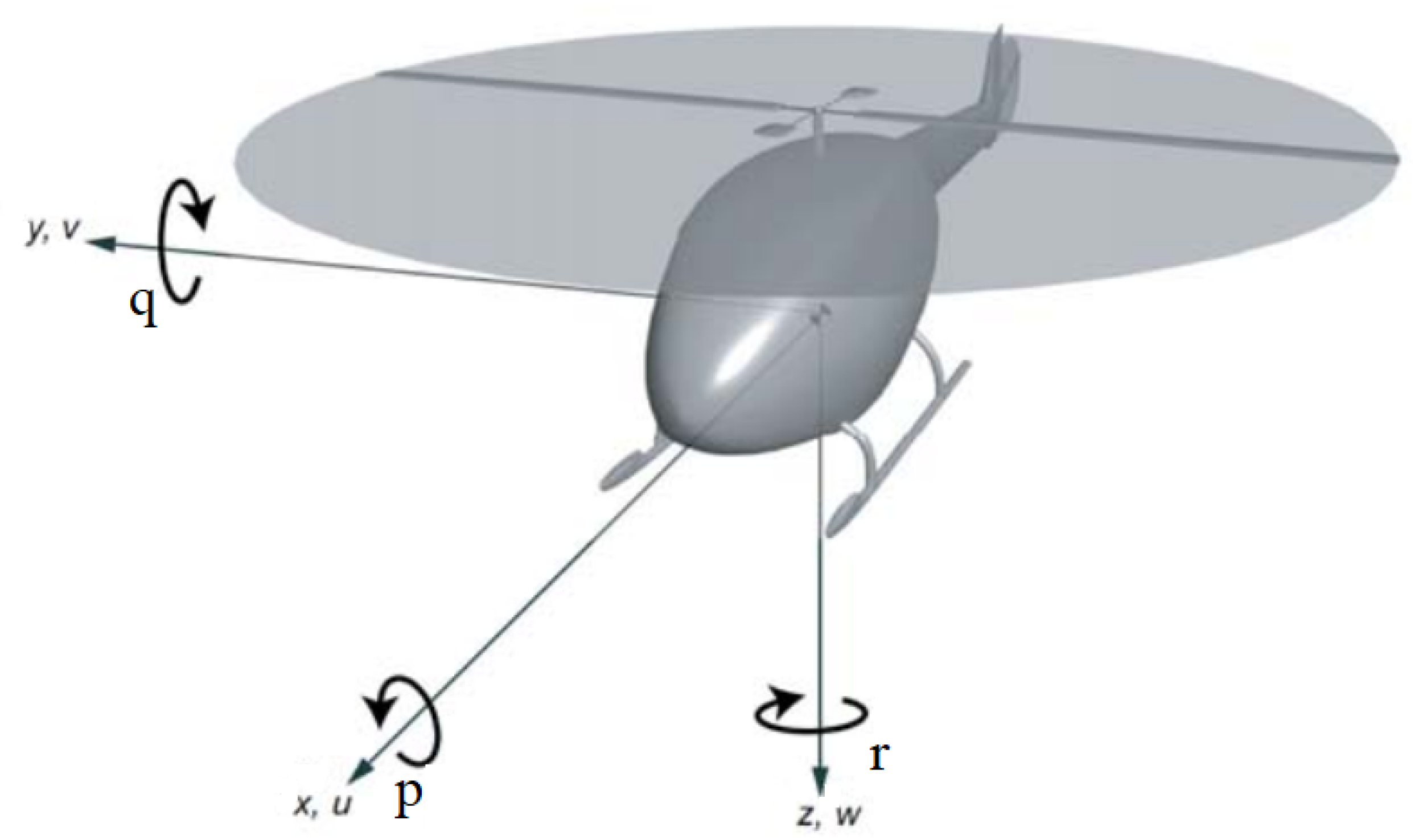
2. Helicopter Nonlinear Dynamic Model

In this section, a precise flight dynamic model has been presented for a small-scale UAV called Yamaha R-50 [8]. To achieve the best attitude approximation of the helicopter, a six DoF rigid-body dynamic model is employed. Based on Figure 1, the state space equations of the helicopter model are described below

$$\begin{array}{c}\dot{p}=pq\frac{(I_x+I_z-I_y)}{I}+qr\frac{I_y{I}_z-I_z^2-I_{xz}^2}{I}+\frac{I_z}{I}O+\frac{I_{xz}}{I}K\end{array}$$

(1)

$$\begin{array}{c}\dot{q}=(r^2-p^2)\frac{I_{xz}}{I_y}+pr\frac{(I_z-I_x)}{I_y}+\frac{J}{I_y}\end{array}$$

(2)

$$\begin{array}{c}\dot{r}=pq\frac{I_x^2+I_{xz}^2-I_x{I}_y}{I}+qr\frac{(I_y-Ix-I_z)I_{xz}}{I}+\frac{I_{xz}}{I}J+\frac{I_x}{I}K\end{array}$$

(3)

$$\begin{array}{c}I=I_x{I}_z-I_{xz}^2\end{array}$$

(4)

where O, J, and K are the rolling, pitching, and yawing moments, respectively. The states of this dynamic model p, q, and r are roll, pitch, and yaw rates related to the body-fixed frame. The parameter I indicates the moments of inertia. In addition, the states describing the associated angles with the roll, pitch, and yaw are defined as follows

$$\begin{array}{c}\dot{\alpha }=p+qcos\alpha tan\beta +rcos\alpha tan\beta \hfill \end{array}$$

(5)

$$\begin{array}{c}\dot{\beta }=qcos\alpha -rsin\alpha \end{array}$$

(6)

$$\begin{array}{c}\dot{\gamma }=qcos\alpha sec\beta +rcos\alpha sec\beta \end{array}$$

(7)

where $\alpha$, $\beta$, and $\gamma$ are the angle of the roll, pitch, and yaw, respectively. In this model, $\theta$ and $\varphi$ are known as lateral and longitudinal flapping angles, respectively, which can be defined as

$$\begin{array}{c}\dot{\theta }=-\frac{nm}{16}\theta -q+\frac{n}{16}p-\frac{nm}{16}{L}_{long}\end{array}$$

(8)

$$\begin{array}{c}\dot{\varphi }=-\frac{nm}{16}\varphi -p+\frac{n}{16}q-\frac{nm}{16}{L}_{lat}\end{array}$$

(9)

where n is the blade lock number which explains the aerodynamic forces and the blade inertia moments rate. The rotational speed of the rotor is indicated by m.

This helicopter is supposed to be controlled by a remote controller. Regarding Equation (10), the control vector of this remote controller consists of four inputs.

$$\begin{array}{c}v=\left[L_{lat}{L}_{long}{L}_{ped}{L}_{col}\right]\end{array}$$

(10)

UAVs have four main control inputs, which are lateral cyclic ($L_{lat}$), longitudinal cyclic ($L_{long}$), collective cyclic ($L_{col}$), and the collective pedal input of tail rotor ($L_{ped}$) used to control yawing moment. In this paper, to indicate the relation between the remote controller vector, v, and the moments of UAV, a simplified model of the rotor aerodynamics during hovering situation is employed [17] and described as

$$\begin{array}{c}O=o_{lat}{L}_{lat}+o_{long}{L}_{long}+o_{ped}{L}_{ped}+o_0\\ J=j_{lat}{L}_{lat}+j_{long}{L}_{long}+j_{ped}{L}_{ped}+j_0\\ K=k_{lat}{L}_{lat}+k_{long}{L}_{long}+k_{ped}{L}_{ped}+k_0\end{array}$$

(11)

where $o_{lat}$, $j_{lat}$, and $k_{lat}$ relate the lateral moment to the lateral remote controller input, $L_{lat}$. In addition, $o_{long}$, $j_{long}$, and $k_{long}$ relate the longitudinal moment to the longitudinal remote controller input $L_{lat}$. In addition, $o_{ped}$, $j_{ped}$ and $k_{ped}$ are related to the pedal collective remote controller input $L_{ped}$. The initial momentum values are shown as $o_0$, $j_0$, and $k_0$. The UAV model parameters are defined in

Table 1. The helicopter model parameters definition.

Parameter	Description
$p,q,r$	Roll, pitch, and yaw rates [rad/s]
$\alpha ,\beta ,\gamma$	Roll, pitch, and yaw angles [rad]
$\theta ,\varphi$	Lateral, and longitudinal flapping angle [rad]
O, J, K	Rolling, pitching, and yawing moments [rad]
n	Blade lock number
m	Rotational speed of rotor
v	Remote controller commands vector
$L_{lat}$	Lateral cyclic inputs [rad]
$L_{long}$	Longitudinal cyclic inputs [rad]
$L_{ped}$	Pedal collective inputs of tail rotor [rad]
$L_{col}$	Collective inputs of tail rotor [rad]
$o_{lat}$, $j_{lat}$, $k_{lat}$	Lateral moment to $L_{lat}$
$o_{long}$, $j_{long}$, $k_{long}$	Longitudinal moment to $L_{long}$
$o_{ped}$, $j_{ped}$, $k_{ped}$	Pedal collective moment to $L_{ped}$
$o_0$, $j_0$, $k_0$	Initial momentum values
$I_x,I_y,I_z$	Moments of inertia [kg.m${}^2$]
$I_{xz}$	moment of inertia around $xz$ plane

. Considering the rotor aerodynamics model for a hovered UAV, not only the cost of data collecting is decreased but also the accuracy of moments measurement is boosted [18].

3. Neural Network, EKF Adaptive Approach

Active fault-tolerant control algorithms are based on an online fault detection and diagnostic (FDI) method employed to update the controlling system. This method is responsible for distinguishing faults by analyzing the system’s data. This paper presents an FDI strategy based on a neural network algorithm updating EKF algorithm. The neural network adaptive structure is used to control the proposed helicopter dynamic model.

3.1. Neural Network Adaptive Structure

In complex nonlinear and naturally unstable dynamic systems such as helicopters, any probable fault can significantly impact the desired performance, leading to a system failure. Moreover, considering the random nature of nonlinear faults, it is challenging to predict them. In recent decades, remarkable methods are introduced in the field of fault detection [19,20,21,22,23]. Regarding these methods, the adaptive neural network algorithm shows a powerful capability in estimating the fault behavior [24,25,26]. The neural network adaptive structure (NNAS) detects faults based on the nonlinear observer output. In contrast, the adaptive neural network (ANN) tries to predict the behavior of the nonlinear system [27]. Equation (12) describes the state space equation of a nonlinear system with additive noise and adaptive neural network as follows

$$\begin{array}{c}\dot{\widehat{x}}=f\left(\widehat{x}\left(t\right)\right)+g\left(\widehat{x}\left(t\right)\right)u\left(t\right)+\zeta \left(t\right)\\ \widehat{y}=h\left(\widehat{x}\left(t\right)\right)\end{array}$$

(12)

where $\widehat{y}$ is the observer’s output vector, $\widehat{x}\left(t\right)$ indicates the state space vector of the nonlinear observer, and $\zeta \left(t\right)$ presents the neural network observer as

$$\begin{array}{c}{\zeta }_i\left(t\right)=M_i\left(t\right)\sigma \left(N_i\left(t\right){\lambda }_i\left(t\right)\right),i=1,...,b\\ suchthat:\sigma \left(x\right)=\frac{1-e^{-x}}{1+e^{-x}}\\ N_i\left(t\right)=[N_{i,1}\left(t\right),...,N_{i,a+b}\left(t\right)]\\ {\lambda }_i\left(t\right)={[{\zeta }_i(t-\tau ),...,{\zeta }_i(t-a\tau ),e_i(t-\tau ),...,e_i(t-b\tau )]}^T\\ e_i\left(t\right)=y_i\left(t\right)-{\widehat{y}}_i\left(t\right)\end{array}$$

(13)

where ${\zeta }_i\left(t\right)$ is the $i^{th}$ vector of $\zeta \left(t\right)$. $M_i\left(t\right)$ and $N_i\left(t\right)$ are presenting the weights of $i^{th}$ output of the neural network algorithm. $\tau$ is the observer step size that is defined as the sampling period. In addition, Equation (14) defines the $N_i\left(t\right){\lambda }_i\left(t\right)$ value as

$$\begin{array}{c}{N}_i\left(t\right){\lambda }_i\left(t\right)=\sum _{j=1}^a{N}_{i,j}\left(t\right){\zeta }_i(t-j\tau )+\sum _{j=1}^b{N}_{i,a+j}\left(t\right)e_i(t-j\tau )\end{array}$$

(14)

where a and b are the weight parameters in the neural network algorithm tuning the algorithm’s accuracy and calculation time. More values of a and b lead to more accuracy in the neural network algorithm [28]. Although increasing the neural network weights ensures the method’s convergence, the calculation time will be increased due to more required computation. Therefore, optimizing the neural network algorithm’s weight parameters should be based on the required accuracy and response time.

3.2. EKF and Neural Network Weight Update

The extended Kalman filter is an estimation method that can be employed to optimize the weight parameters in the neural network algorithm. Employing the EKF for tuning the weights parameters helps decrease the neural network computation time. This could make it possible to apply this algorithm in a real-time problem. To apply the EKF, an update parameter should be considered as [29]

$$\begin{array}{c}{E}_i\left(k\right)={[N_i\left(k\right),{\zeta }_{i,1}\left(k\right),...,{\zeta }_{i,a+b}\left(k\right)]}^T\end{array}$$

(15)

where $E_i\left(k\right)$ indicates the EKF updating parameters for the $k^{th}$ sampling instant and the $i^{th}$ element of the neural network adaptive structure algorithm. To calculate each updated parameter for the $k^{th}$ sample, $E_i\left(k\right)$ can be reformulated as

$$\begin{array}{c}{E}_i\left(k\right)=E_i(k-1)+l_i{K}_i\left(k\right)[y_i\left(k\right)-{\widehat{y}}_i\left(k\right)]\end{array}$$

(16)

where $l_i$ is the learning coefficient and $K_i\left(k\right)$ shows the Kalman gain in the EKF algorithm. The Kalman gain is calculated as below

$$\begin{array}{c}{K}_i\left(k\right)=C_i^e\left(k\right)D_i\left(k\right){[D_i{\left(k\right)}^T{C}_i^e\left(k\right)D_i\left(k\right)+C_i^b\left(k\right)]}^{-1}\\ D_i\left(k\right)=\frac{\partial e_i\left(k\right)}{\partial E_i}{|}_{E_i=E_i(k-1)}\end{array}$$

(17)

where $C_i^e\left(k\right)$ is the state estimation error covariance matrix, and $C_i^b\left(k\right)$ is the estimated noise covariance matrix. In order to calculate the covariance matrices, a recursive approach is employed [30] and formulated as

$$\begin{array}{c}{C}_i^e(k+1)=C_i^e\left(k\right)-K_i\left(k\right)D_i^T\left(k\right)C_i^e\left(k\right)\\ C_i^b\left(k\right)=C_i^b(k-1)+\frac{e_i^T\left(k\right)e_i\left(k\right)-C_i^b(k-1)}{k}.\end{array}$$

(18)

Considering Equations (13) and (17), $D_i\left(k\right)$ can be computed as below

$$\begin{array}{c}{D}_i\left(k\right)=\left\{\begin{array}{cc}\sigma \left(N_i\left(k\right){\lambda }_i\left(k\right)\right)\hfill & E_i=M_i\\ M_i\left(k\right)\zeta (k-j)\acute{\sigma }\left(N_i\left(k\right){\lambda }_i\left(k\right)\right)\hfill & E_i=N_{i,j}\\ M_i\left(k\right)e(k-j)\acute{\sigma }\left(N_i\left(k\right){\lambda }_i\left(k\right)\right)\hfill & E_i=N_{i,a+j}.\end{array}\right.\end{array}$$

(19)

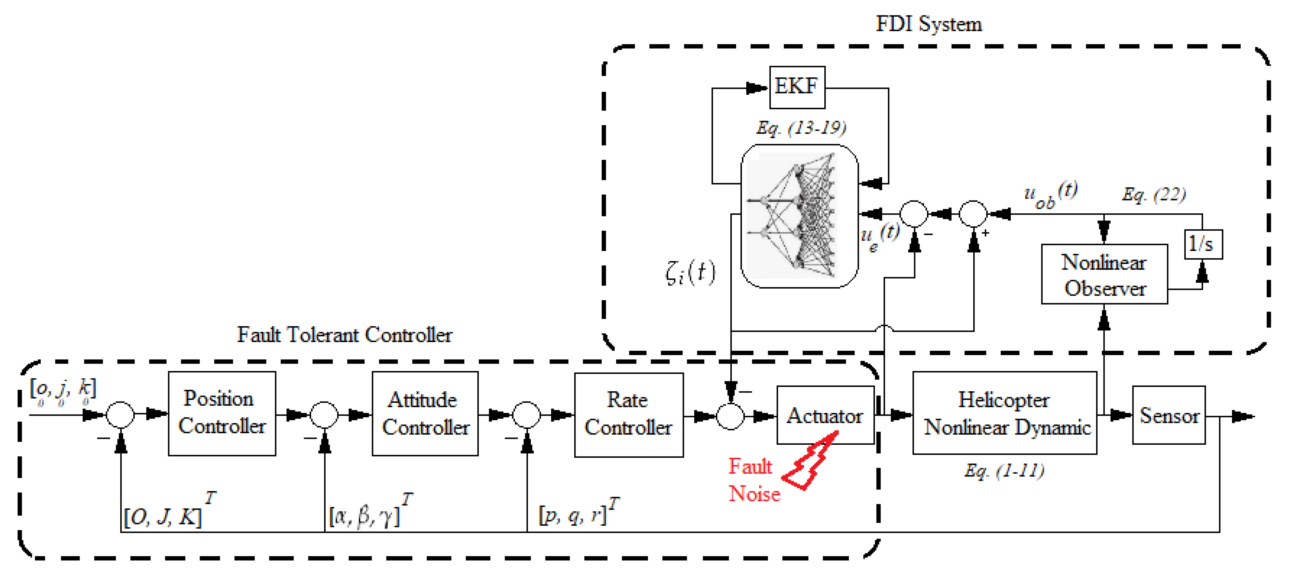
3.3. Fault Detection and Diagnostic Design for Actuator

The actuator in the dynamic system of a helicopter plays a critical role in the control of its attitude. This component requires the fastest response to the operator commands. Therefore, the fault detection and controlling procedure should be processed in a required amount of time to maintain the actuator performance successfully. To indicate the motion equations of the helicopter angular rate with actuator disturbances, we have

$$\begin{array}{c}\dot{x}=f\left(x\right)+g_{in}\left(x\right)u\left(t\right)+\omega \left(t\right)\\ x={\left[pqr\right]}^T\end{array}$$

(20)

where $\omega \left(t\right)$ is the actuator fault, $f\left(x\right)$ and $g\left(x\right)$ can be derived from Equations (1)–(3) as

$$\begin{array}{c}f\left(x\right)={\left[f_p\left(x\right)f_q\left(x\right)f_r\left(x\right)\right]}^T=\left[\begin{array}{c}pq\frac{(I_x+I_z-I_y)I_{xz}}{I}+qr\frac{I_y{I}_z-I_z^2-I_{xz}^2}{I}+{\frac{I_z}{I}}_{j_0}\\ (r^2-q^2)\frac{I_{xz}}{I_y}+pr\frac{I_z-I_x}{I_y}+\frac{1}{I_y}{o}_0\\ pq\frac{I_x^2+I_{xz}^2-I_x{I}_y}{I}+qr\frac{(I_y-I_x-I_z)I_{xz}}{I}+\frac{I_{xz}}{I}{j}_0+\frac{I_x}{I}{y}_0\end{array}\right]\\ g_{in}\left(x\right)={\left[\begin{array}{ccc}\frac{I_z}{I}{j}_{lat}+\frac{I_{xz}}{I}{k}_{lat}\hfill & \frac{o_{lat}}{I_y}& \frac{I_{xz}}{I}{j}_{lat}+\frac{I_x}{I}{k}_{lat}\\ \frac{I_z}{I}{j}_{long}+\frac{I_{xz}}{I}{k}_{long}\hfill & \frac{o_{long}}{I_y}& \frac{I_{xz}}{I}{j}_{long}+\frac{I_x}{I}{k}_{long}\\ \frac{I_z}{I}{j}_{ped}+\frac{I_{xz}}{I}{k}_{ped}\hfill & \frac{o_{ped}}{I_y}& \frac{I_{xz}}{I}{j}_{ped}+\frac{I_x}{I}{k}_{ped}\end{array}\right]}^T.\end{array}$$

(21)

Finally, considering the above equations, fault detection and isolation design for the helicopter actuators can be described as

$$\begin{array}{c}{u}_{ob}=g_{in}^{-1}\left(x\right)(\dot{x}-f\left(x\right))\\ u_e=u-(u_{ob}+{\zeta }_i\left(t\right))\end{array}$$

(22)

where $u_{ob}$ and $u_e$ are the nonlinear observer model of the actuator and the error in the fault detection procedure, respectively. In addition, u is defined in Equation (28). ${\zeta }_i$ updated by the sampling period can be formulated as

$$\begin{array}{c}{\zeta }_i(k+1)=M_i\sigma \left(\sum _{j=1}^a{N}_{i,j}{\zeta }_i(k-j+1)+Z_i\left(k\right)\right)\\ Z_i\left(k\right)=\sum _{j=1}^b{N}_{i,a}+e_i(k-j+1).\end{array}$$

(23)

To explain the updating process of the proposed method, Figure 2 shows the flowchart of updating the NN parameters.

4. Active Fault Tolerant Control Strategy

In the control design of a UAV attitude, an accurate and fast fault detection method is essential, but a reliable controller is required to filter the detected faults. In this paper, the proposed controller is divided into two main feedbacks. The first feedback controller, known as nonlinear dynamic inversion controller, consists of two inner and outer loops. The second feedback is the adaptive fault compensation controller.

4.1. First Feedback Controller: Nonlinear Dynamic Inversion

Nonlinear dynamic inversion can control the helicopter attitude by feedback linearization technique [12]. This method consists of two control loops, which have to be completely different in frequency bandwidth to prevent any probable interaction [31]. Hence, the state dynamics should be controlled by inner and outer control loops that have faster and slower responses, respectively.

In the helicopter control system, the six DoF controller model can be formulated as [32]

$$\ddot{x}=f(x,\dot{x},\kappa )$$

(24)

$$\widehat{\kappa }={\widehat{f}}^{-1}(x,\dot{x},\ddot{\widehat{x}})$$

(25)

where x and $\dot{x}$ are state variables and f is the invertible mapping function, which transforms control variable $\kappa$ to the state variables. $\widehat{f}$ presents an analytical model for the helicopter dynamics. Therefore, the helicopter control system can be described as

$$\begin{array}{c}\ddot{x}=\ddot{\widehat{x}}+\Gamma (x,\dot{x},\kappa )\\ \Gamma (x,\dot{x},\kappa )=f(x,\dot{x},\kappa )-f^{-1}(x,\dot{x},\ddot{\widehat{x}})\end{array}$$

(26)

where $\Gamma$ is the inversion error.

4.1.1. Inner Control Loop

In the helicopter dynamic model, the fastest states are attitude rates p, q, and r. In addition, the control variables which control the actuator are angular rates $L_{lat}$, $L_{long}$, and $L_{ped}$. Referring to Equations (1)–(3) and (20)–(22), the inner loop dynamics can be described as

$$\begin{array}{c}\left[\begin{array}{c}\dot{p}\hfill \\ \dot{q}\hfill \\ \dot{r}\hfill \end{array}\right]=\left[\begin{array}{c}{f}_p\left(x\right)\hfill \\ f_q\left(x\right)\hfill \\ f_r\left(x\right)\hfill \end{array}\right]+g_{in}\left(x\right)\left[\begin{array}{c}{L}_{lat}\hfill \\ L_{long}\hfill \\ L_{ped}\hfill \end{array}\right]\end{array}$$

(27)

where $f_p$, $f_q$, $f_r$, and $g_{in}\left(x\right)$ are presented in Equations (20)–(22). Considering the desired angular rates, the inner loop controller can be defined as

$$\begin{array}{c}u=\left[\begin{array}{c}{L}_{lat}\hfill \\ L_{long}\hfill \\ L_{ped}\hfill \end{array}\right]=g_{in}^{-1}\left(x\right)\left(\left[\begin{array}{c}{\dot{p}}_d\hfill \\ {\dot{q}}_d\hfill \\ {\dot{r}}_d\hfill \end{array}\right]-\left[\begin{array}{c}{f}_p\left(x\right)\hfill \\ f_q\left(x\right)\hfill \\ f_r\left(x\right)\hfill \end{array}\right]\right)\end{array}$$

(28)

$$\begin{array}{c}\left[\begin{array}{c}{\dot{p}}_d\hfill \\ {\dot{q}}_d\hfill \\ {\dot{r}}_d\hfill \end{array}\right]=\left[\begin{array}{ccc}{\omega }_p\hfill & 0& 0\\ 0\hfill & {\omega }_q& 0\\ 0\hfill & 0& {\omega }_r\end{array}\right]\left[\begin{array}{c}{p}_r-p\hfill \\ q_r-q\hfill \\ r_r-r\hfill \end{array}\right]\end{array}$$

(29)

where ${\dot{p}}_d$, ${\dot{q}}_d$, ${\dot{r}}_d$ are desired angular rates. $p_r$, $q_r$, $r_r$ are the received angular rate from the outer loop. ${\omega }_p$, ${\omega }_q$, ${\omega }_r$ are the inner loop gains selected by the designer to reach the desired goal. To guarantee the stability of the of $g_{in}\left(x\right)$ and its inverse matrix $g_{in}^{-1}\left(x\right)$, inner-loop gains should be chosen sufficiently large [33]. In this way, we can guarantee that the determinant of g(x) will never merge to zero and its inverse will be stabilized and bounded.

4.1.2. Outer Control Loop

To control the slow states of the helicopter, $\alpha$, $\beta$, and $\gamma$, the outer loop receives input commands ${\alpha }_i$, ${\beta }_i$, and ${\gamma }_i$ from the guidance system and sends the outputs $p_r$, $q_r$, and $r_i$ as the reference commands to the inner-loop controller. The assumption of the time-scale separation between the inner-loop and the outer-loop controllers ensures that the deflections of the control surfaces $L_{lat}$, $L_{long}$, and $L_{ped}$ have no interaction with the outer-loop states. Considering Equations (5)–(7), the outer-loop states can be described as

$$\begin{array}{c}\left[\begin{array}{c}\dot{\alpha }\hfill \\ \dot{\beta }\hfill \\ \dot{\gamma }\hfill \end{array}\right]=\left[\begin{array}{c}{f}_{\alpha }\left(x\right)\hfill \\ f_{\beta }\left(x\right)\hfill \\ f_{\gamma }\left(x\right)\hfill \end{array}\right]+g_{out}\left(x\right)\left[\begin{array}{c}p\hfill \\ q\hfill \\ r\hfill \end{array}\right]\end{array}$$

(30)

where the concepts of functions f and g are defined in Equations (21) and (22). In order to obtain the desired slow states, the outer-loop controller is defined as below

$$\begin{array}{c}\left[\begin{array}{c}{p}_r\hfill \\ q_r\hfill \\ r_r\hfill \end{array}\right]=g_{out}^{-1}\left(x\right)\left(\left[\begin{array}{c}{\dot{\alpha }}_d\hfill \\ {\dot{\beta }}_d\hfill \\ {\dot{\gamma }}_d\hfill \end{array}\right]-\left[\begin{array}{c}{f}_{\alpha }\left(x\right)\hfill \\ f_{\beta }\left(x\right)\hfill \\ f_{\gamma }\left(x\right)\hfill \end{array}\right]\right)\end{array}$$

(31)

$$\left[\begin{array}{c}{\dot{\alpha }}_d\hfill \\ {\dot{\beta }}_d\hfill \\ {\dot{\gamma }}_d\hfill \end{array}\right]=\left[\begin{array}{ccc}{\omega }_{\alpha }\hfill & 0& 0\\ 0\hfill & {\omega }_{\beta }& 0\\ 0\hfill & 0& {\omega }_{\gamma }\end{array}\right]\left[\begin{array}{c}{\alpha }_i-\alpha \hfill \\ {\beta }_i-\beta \hfill \\ {\gamma }_i-\gamma \hfill \end{array}\right]$$

(32)

where ${\omega }_{\alpha }$, ${\omega }_{\beta }$, ${\omega }_{\gamma }$ are the outer-loop gains selecting by the designer to reach the desired goal.

4.2. Adaptive Fault Compensator Design

Disturbances in the dynamic system of a helicopter can be detected and controlled by the proposed controller. Moreover, to compensate for the system’s error, this controller, including a nonlinear dynamic inversion and an adaptive neural network structure, employs a real-time feedback command. This fault-tolerant control design can be formulated as

$$\begin{array}{c}\left[\begin{array}{c}\dot{p}\hfill \\ \dot{q}\hfill \\ \dot{r}\hfill \end{array}\right]=\left[\begin{array}{c}{f}_p\left(x\right)\hfill \\ f_q\left(x\right)\hfill \\ f_r\left(x\right)\hfill \end{array}\right]+g_{in}\left(x\right)\left[\begin{array}{c}{L}_{lat}\hfill \\ L_{long}\hfill \\ L_{ped}\hfill \end{array}\right]+\omega \left(t\right)-f_a\left(t\right)\end{array}$$

(33)

$$\begin{array}{c}\left[\begin{array}{c}{L}_{lat}\hfill \\ L_{long}\hfill \\ L_{ped}\hfill \end{array}\right]=g_{in}^{-1}\left(x\right)\times \left(\left[\begin{array}{c}{\dot{p}}_d\hfill \\ {\dot{q}}_d\hfill \\ {\dot{r}}_d\hfill \end{array}\right]-\left[\begin{array}{c}{f}_p\left(x\right)\hfill \\ f_q\left(x\right)\hfill \\ f_r\left(x\right)\hfill \end{array}\right]+\omega \left(t\right)-f_a\left(t\right)\right)\end{array}$$

(34)

where $\omega \left(t\right)$ is the actuator fault and $f_a\left(t\right)$ indicates the neural network compensator for the system disturbances.

Figure 3 illustrates the framework of the proposed method. This figure indicates the interconnection between the FDI system and the active FTC.

5. Implementation of the Proposed Method on Helicopter

The helicopter can be affected by noises on the part of sensor measurements and actuators. In order to test the neural network’s reliability, the EKF adaptive algorithm, the rolling, pitching, and yawing rates of the helicopter are affected by three separated abrupt, incipient, and intermittent faults.

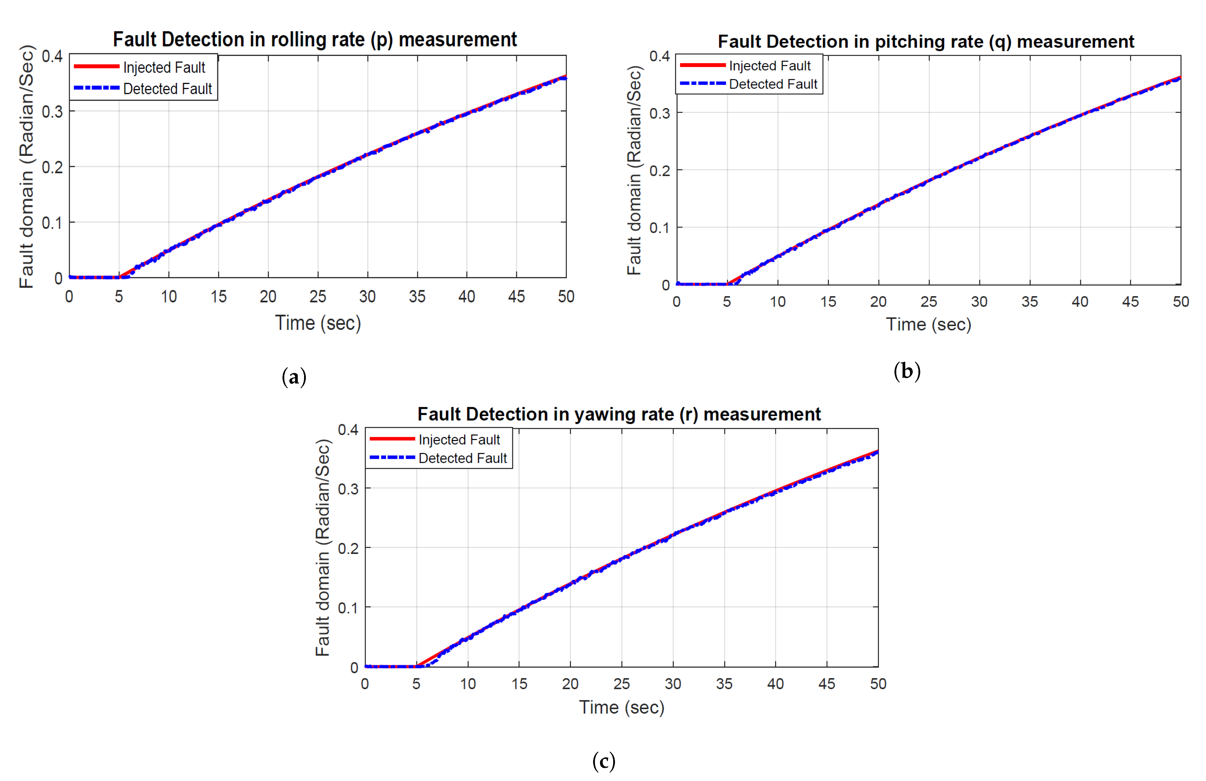
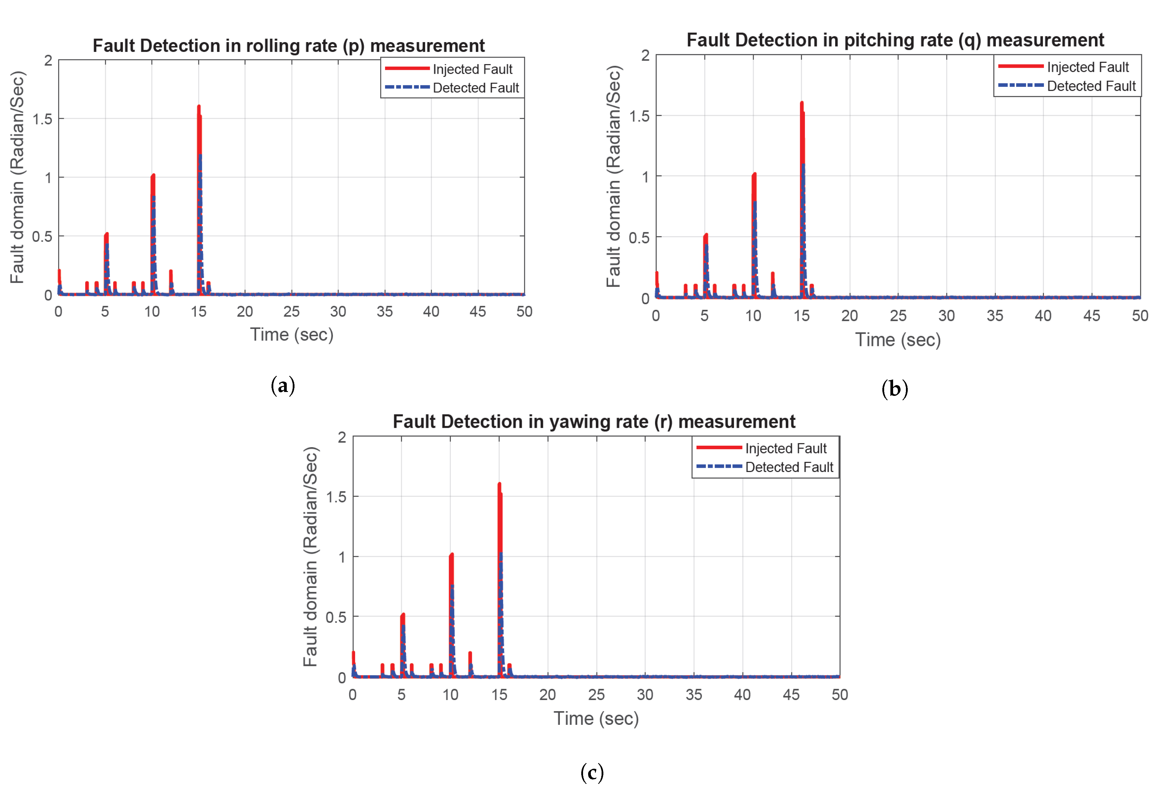
5.1. Faults Description

Sensors and actuators used in unmanned helicopters can be affected in various methods. Some faults can occur in various parts, while others would affect a particular sensor or actuator [34]. In this paper, the following faults are considered.

5.1.1. Abrupt Faults

During the helicopter’s operation, a parameter value may shift faster than the nominal dynamic process due to electrical or communication problems. These problems can result from the helicopter vibrations, short circuits, or metal flake separating.

5.1.2. Incipient Faults

Incipient faults are complicated to be detected, and they could cause severe problems leading to system failure. Detection of incipient faults requires an advanced fault detection and diagnosis (FDD) algorithm [35]. A partial sensor failure is typically the primary cause of an incipient fault [28]. This fault can be mathematically modeled [36] by Equation (35) as below

$$\begin{array}{c}Fault(t-\tau )=1-e^{-w(t-\tau )}fort⩾\tau \end{array}$$

(35)

where w shows an unknown fault evaluation rate. A small amount of w leads to a slightly increasing slope called incipient faults, while a large amount of w results in a step shape fault known as a sudden fault.

5.1.3. Intermittent Faults

Intermittent faults are not easily repeatable because of their complicated behavioral patterns but can affect the system due to any sensor’s malfunction at irregular intervals. This kind of fault is notoriously difficult to identify since it occurs for a short period of time.

5.2. Numerical Simulation

In this paper, the test-bed is the model of the Yamaha R-50 small-scale unmanned helicopter. The neural network EKF adaptive algorithm is applied to this model to show the proposed method’s reliability during operation. The following assumptions are made to achieve the most optimized outcome:

(1)

The helicopter blade is twisted along the length of the blade due to the unbalanced lift compensation.

(2)

The helicopter rotors are assumed as teetering rotors. This means the blades flap without any curve.

(3)

Since the wind speed is presumed to be zero and the air density is constant, there is no external force on the helicopter body.

(4)

Table 2. Rotor aerodynamics parameters [37].

Parameter	Value	Parameter	Value	Parameter	Value
$o_{lat}$	39.51	$j_{lat}$	−8.54	$k_{lat}$	0.0013
$o_{long}$	8.54	$j_{long}$	39.51	$k_{long}$	0.0013
$o_{ped}$	0.73	$j_{ped}$	−0.064	$k_{ped}$	−9.24
$o_0$	0.044	$j_0$	−0.47	$k_0$	0.73

shows the used parameters for the rotor aerodynamics in the helicopter model simulation.

Three different faults explained in the previous subsection are injected into the rolling rate (p), pitching rate (q), and yawing rate (r) of the unmanned helicopter sensors. The simulation results shown in Figure 4, Figure 5 and Figure 6 demonstrate the proposed algorithm’s ability to detect a wide range of possible system faults. The obtained results prove that the algorithm is reliable enough to be applied for the proposed active FTC design and to guarantee an unmanned helicopter’s performance during hovering in the presence of faults. In order to prove the fault tolerance capability of the proposed FTC design, a circular trajectory, as shown in Figure 7, is implemented to the helicopter. The abrupt fault is injected into the rolling, pitching, and yawing rates for 20 seconds of the simulation, as shown in Figure 4. The result of the proposed FTC design is compared with a nonlinear dynamic inversion controller. As Figure 7 shows, the proposed controller is able to mitigate the injected fault and track the commanded trajectory with sufficient accuracy.

6. Conclusions

This paper introduced a novel technique for detecting and mitigating fault and false data injected attacks in the sensors and actuators of an unmanned helicopter using NN and EKF. In the proposed algorithm, a combination of a model-based observer and an adaptive NN is used to detect and isolate faults. This combination is used due to its independence to training data and robustness against uncertainties in the model-based observer. To further improve the detection system’s accuracy, the EKF is introduced to tune the neural network weights. In order to test the efficiency of this algorithm, a nonlinear dynamic model of a small unmanned helicopter named Yamaha R-50 is employed. The simulation results show that this method can appropriately identify three distinct faults. These three fault categories are abrupt, incipient, and intermittent faults, which cover the most significant potential analytical faults in the navigation sensors during a helicopter flight domain. Then, based on the designed detection system, an active fault-tolerant control system is designed to mitigate the detected faults/false data. The effectiveness of the proposed design has been tested and evaluated through the different simulation scenarios. The proposed algorithm improves the reliability and safety of unmanned systems and prevents catastrophic incidents caused by faulty sensors.

In the future study, the proposed FTC method could be applied to a real UAV to evaluate its application in real life. In addition, the application of this method can be applied to other UAVs such as drones to investigate its reliability on similar nonlinear dynamic systems. Moreover, while in this study the EKF is used to regulate the NN weights, it is possible to use other algorithms in this regard, such as the unscented Kalman filter (UKF).

The following abbreviations are used in this manuscript:

References

1. Chen, M.; Shi, P.; Lim, C.C. Adaptive neural fault-tolerant control of a 3-DOF model helicopter system. IEEE Trans. Syst. Man Cybern. Syst. 2015, 46, 260–270. [Google Scholar] [CrossRef] [Green Version]
2. Gustafsson, F. Statistical Sensor Fusion, 1st ed.; Studentlitteratur: Lund, Sweden, 2010. [Google Scholar]
3. Arafat, M.; Nafis, S.R.; Sadeghvaziri, E.; Tousif, F. A data-driven approach to calibrate microsimulation models based on the degree of saturation at signalized intersections. Transp. Res. Interdiscip. Perspect. 2020, 8, 100231. [Google Scholar] [CrossRef]
4. Hadi, M.; Iqbal, M.S.; Wang, T.; Xiao, Y.; Arafat, M.; Afreen, S. Connected Vehicle Vehicle-to-Infrastructure Support of Active Traffic Management; National Transportation Library: Washington, DC, USA, 2019. [Google Scholar]
5. Zhu, H.; Peng, X.; Chandrasekhar, V.; Li, L.; Lim, J.H. DehazeGAN: When Image Dehazing Meets Differential Programming. In Proceedings of the International Joint Conference on Artificial Intelligence, Stockholm, Sweden, 13–19 July 2018; pp. 1234–1240. [Google Scholar]
6. Zhou, J.T.; Di, K.; Du, J.; Peng, X.; Yang, H.; Pan, S.J.; Tsang, I.; Liu, Y.; Qin, Z.; Goh, R.S.M. Sc2net: Sparse lstms for sparse coding. In Proceedings of the AAAI Conference on Artificial Intelligence, New Orleans, LA, USA, 2–7 February 2018; Volume 32. [Google Scholar]
7. Liu, Y.J.; Li, J.; Tong, S.; Chen, C.P. Neural network control-based adaptive learning design for nonlinear systems with full-state constraints. IEEE Trans. Neural Netw. Learn. Syst. 2016, 27, 1562–1571. [Google Scholar] [CrossRef]
8. Abaspour, A.; Sadati, S.H.; Sadeghi, M. Nonlinear optimized adaptive trajectory control of helicopter. Control. Theory Technol. 2015, 13, 297–310. [Google Scholar] [CrossRef]
9. Dalamagkidis, K.; Valavanis, K.P.; Piegl, L.A. Nonlinear model predictive control with neural network optimization for autonomous autorotation of small unmanned helicopters. IEEE Trans. Control. Syst. Technol. 2010, 19, 818–831. [Google Scholar] [CrossRef]
10. Kadmiry, B.; Driankov, D. A fuzzy gain-scheduler for the attitude control of an unmanned helicopter. IEEE Trans. Fuzzy Syst. 2004, 12, 502–515. [Google Scholar] [CrossRef]
11. Afshar, S.; Wasti, S.; Disfani, V. Coordinated EV Aggregation Management via Alternating Direction Method of Multipliers. In Proceedings of the 2020 International Conference on Smart Grids and Energy Systems (SGES), Perth, Australia, 23–26 November 2020; pp. 882–887. [Google Scholar]
12. Abbaspour, A.; Yen, K.K.; Forouzannezhad, P.; Sargolzaei, A. A neural adaptive approach for active fault-tolerant control design in uav. IEEE Trans. Syst. Man Cybern. Syst. 2018, 50, 3401–3411. [Google Scholar] [CrossRef]
13. Mokhtari, S.; Yen, K.K. A Novel Bilateral Fuzzy Adaptive Unscented Kalman Filter and its Implementation to Nonlinear Systems with Additive Noise. In Proceedings of the 2020 IEEE Industry Applications Society Annual Meeting, Detroit, MI, USA, 10–16 October 2020; pp. 1–6. [Google Scholar] [CrossRef]
14. Abbaspour, A.; Mokhtari, S.; Sargolzaei, A.; Yen, K.K. A Survey on Active Fault-Tolerant Control Systems. Electronics 2020, 9, 1513. [Google Scholar] [CrossRef]
15. Park, P.; Khadilkar, H.; Balakrishnan, H.; Tomlin, C.J. High Confidence Networked Control for Next Generation Air Transportation Systems. IEEE Trans. Autom. Control. 2014, 59, 3357–3372. [Google Scholar] [CrossRef] [Green Version]
16. Rudin, K.; Ducard, G.J.; Siegwart, R.Y. Active Fault Tolerant Control with Imperfect Fault Detection Information: Applications to UAVs. IEEE Trans. Aerosp. Electron. Syst. 2019, 56, 2792–2805. [Google Scholar] [CrossRef]
17. Zeng, S.; Zhu, J. Adaptive compensated dynamic inversion control for a helicopter with approximate mathematical model. In Proceedings of the 2006 International Conference on Computational Inteligence for Modelling Control and Automation and International Conference on Intelligent Agents Web Technologies and International Commerce (CIMCA’06), Sydney, Australia, 28 November–1 December 2006; p. 208. [Google Scholar]
18. Ren, B.; Ge, S.S.; Chen, C.; Fua, C.H.; Lee, T.H. Modeling, Control and Coordination of Helicopter Systems; Springer Science & Business Media: Berlin/Heidelberg, Germany, 2012. [Google Scholar]
19. Sreedhar, R.; Fernandez, B.; Masada, G.Y. Robust fault detection in nonlinear systems using sliding mode observers. In Proceedings of the IEEE International Conference on Control and Applications, Vancouver, BC, Canada, 13–16 September 1993; pp. 715–721. [Google Scholar]
20. Mokhtari, S.; Abbaspour, A.; Yen, K.K.; Sargolzaei, A. A Machine Learning Approach for Anomaly Detection in Industrial Control Systems Based on Measurement Data. Electronics 2021, 10, 407. [Google Scholar] [CrossRef]
21. Li, L.; Ding, S.X.; Yang, Y.; Peng, K.; Qiu, J. A fault detection approach for nonlinear systems based on data-driven realizations of fuzzy kernel representations. IEEE Trans. Fuzzy Syst. 2017, 26, 1800–1812. [Google Scholar] [CrossRef]
22. Wang, Z.; Liu, L.; Zhang, H. Neural network-based model-free adaptive fault-tolerant control for discrete-time nonlinear systems with sensor fault. IEEE Trans. Syst. Man Cybern. Syst. 2017, 47, 2351–2362. [Google Scholar] [CrossRef]
23. Liu, X.; Han, J.; Zhang, H.; Sun, S.; Hu, X. Adaptive Fault Estimation and Fault-Tolerant Control for Nonlinear System With Unknown Nonlinear Dynamic. IEEE Access 2019, 7, 136720–136728. [Google Scholar] [CrossRef]
24. Kiranyaz, S.; Gastli, A.; Ben-Brahim, L.; Al-Emadi, N.; Gabbouj, M. Real-time fault detection and identification for MMC using 1-D convolutional neural networks. IEEE Trans. Ind. Electron. 2018, 66, 8760–8771. [Google Scholar] [CrossRef]
25. Shen, Q.; Jiang, B.; Shi, P.; Lim, C.C. Novel neural networks-based fault tolerant control scheme with fault alarm. IEEE Trans. Cybern. 2014, 44, 2190–2201. [Google Scholar] [CrossRef]
26. Guo, M.F.; Zeng, X.D.; Chen, D.Y.; Yang, N.C. Deep-learning-based earth fault detection using continuous wavelet transform and convolutional neural network in resonant grounding distribution systems. IEEE Sens. J. 2017, 18, 1291–1300. [Google Scholar] [CrossRef]
27. Kamalasadan, S.; Swann, G.D.; Yousefian, R. A Novel System-Centric Intelligent Adaptive Control Architecture for Power System Stabilizer Based on Adaptive Neural Networks. IEEE Syst. J. 2014, 8, 1074–1085. [Google Scholar] [CrossRef]
28. Abbaspour, A.; Aboutalebi, P.; Yen, K.K.; Sargolzaei, A. Neural adaptive observer-based sensor and actuator fault detection in nonlinear systems: Application in UAV. ISA Trans. 2017, 67, 317–329. [Google Scholar] [CrossRef]
29. Liu, T.; Dai, Y.; Hong, G. Flight dynamic simulation of helicopter forward flight through microburst wind field. Adv. Mech. Eng. 2017, 9, 1687814017691212. [Google Scholar] [CrossRef] [Green Version]
30. Ljung, L.; Söderström, T. Theory and Practice of Recursive Identification; MIT Press: Cambridge, MA, USA, 1983. [Google Scholar]
31. Reiner, J.; Balas, G.J.; Garrard, W.L. Robust dynamic inversion for control of highly maneuverable aircraft. J. Guid. Control. Dyn. 1995, 18, 18–24. [Google Scholar] [CrossRef]
32. Jiang, F.; Pourpanah, F.; Hao, Q. Design, Implementation, and Evaluation of a Neural-Network-Based Quadcopter UAV System. IEEE Trans. Ind. Electron. 2019, 67, 2076–2085. [Google Scholar] [CrossRef]
33. Schumacher, C.; Khargonekar, P.; McClamroch, N. Stability analysis of dynamic inversion controllers using time-scale separation. In Proceedings of the AIAA Guidance, Navigation, and Control Conference and Exhibit, Boston, MA, USA, 10 August–12 August 1998; p. 4322. [Google Scholar]
34. Heredia, G.; Ollero, A. Detection of sensor faults in small helicopter UAVs using observer/Kalman filter identification. Math. Probl. Eng. 2011, 2011, 174618. [Google Scholar] [CrossRef]
35. Naderi, M.S.; Gharehpetian, G.B.; Abedi, M.; Blackburn, T.R. Modeling and detection of transformer internal incipient fault during impulse test. Dielectr. Electr. Insul. IEEE Trans. 2008, 15, 284–291. [Google Scholar] [CrossRef]
36. Zhang, K.; Jiang, B.; Yan, X.G.; Mao, Z. Sliding mode observer based incipient sensor fault detection with application to high-speed railway traction device. ISA Trans. 2016, 63, 49–59. [Google Scholar] [CrossRef]
37. Johnson, E.N.; Kannan, S.K. Adaptive trajectory control for autonomous helicopters. J. Guid. Control. Dyn. 2005, 28, 524–538. [Google Scholar] [CrossRef] [Green Version]
Figure 1. Description of roll, pitch, and yaw in the dynamic helicopter model.
Remotesensing 13 02396 g001
Figure 2. Flowchart of the proposed NN, EKF adaptive algorithm.
Remotesensing 13 02396 g002
Figure 3. Proposed united framework for AFTC diagram of a helicopter.
Remotesensing 13 02396 g003
Figure 4. Abrupt fault detection. (a) Abrupt fault detection in rolling rate measurement. (b) Abrupt fault detection in pitching rate measurement. (c) Abrupt fault detection in yawing rate measurement.
Remotesensing 13 02396 g004
Figure 5. Incipient fault detection. (a) Incipient fault detection in rolling rate measurement. (b) Incipient fault detection in pitching rate measurement. (c) Incipient fault detection in yawing rate measurement.
Remotesensing 13 02396 g005
Figure 6. Intermittent fault detection. (a) Intermittent fault detection in rolling rate measurement. (b) Intermittent fault detection in pitching rate measurement. (c) Intermittent fault detection in yawing rate measurement.
Remotesensing 13 02396 g006
Figure 7. Trajectory tracking in the presence of abrupt fault (Figure 4).
Remotesensing 13 02396 g007