Article

HORUS: Multispectral and Multiangle CubeSat Mission Targeting Sub-Kilometer Remote Sensing Applications

by
Alice Pellegrino
1,
Maria Giulia Pancalli
1,
Andrea Gianfermo
1,
Paolo Marzioli
1,*,
Federico Curianò
2,
Federica Angeletti
1,
Fabrizio Piergentili
1 and
Fabio Santoni
2
1
Department of Mechanical and Aerospace Engineering, Sapienza University of Rome, via Eudossiana 18, 00184 Rome, Italy
2
Department of Astronautical, Electric and Energy Engineering, Sapienza University of Rome, via Eudossiana 18, 00184 Rome, Italy
*
Author to whom correspondence should be addressed.
Remote Sens. 2021, 13(12), 2399; https://0-doi-org.brum.beds.ac.uk/10.3390/rs13122399
Submission received: 3 May 2021 / Revised: 12 June 2021 / Accepted: 13 June 2021 / Published: 19 June 2021

Abstract

:
This paper presents the HORUS mission, aimed at multispectral and multiangle (nadir and off-nadir) planetary optical observation, using Commercial Off-The-Shelf (COTS) instruments on-board a 6-Unit CubeSat. The collected data are characterized by a sub-kilometer resolution, useful for different applications for environmental monitoring, atmospheric characterization, and ocean studies. Latest advancements in electro-optical instrumentation permit to consider an optimized instrument able to fit in a small volume, in principle without significant reduction in the achievable performances with respect to typical large-spacecraft implementations. CubeSat-based platforms ensure high flexibility, with fast and simple components’ integration, and may be used as stand-alone system or in synergy with larger missions, for example to improve revisit time. The mission rationale, its main objectives and scientific background, including the combination of off-nadir potential continuous multiangle coverage in a full perspective and related observation bands are provided. The observation system conceptual design and its installation on-board a 6U CubeSat bus, together with the spacecraft subsystems are discussed, assessing the feasibility of the mission and its suitability as a building block for a multiplatform distributed system.

Graphical Abstract

1. Introduction

Passive methods for spaceborne Earth Observation (EO) used for the analysis of the landscape and environment towards the understanding of natural phenomena rely mostly on the usage of optical-based panchromatic, hyperspectral and multispectral sensors [1,2,3,4,5,6,7,8,9,10].
Panchromatic imaging systems use a single channel detector with a broad sensitivity window, encompassing the entire visible-light spectrum. Panchromatic images offer high-spatial resolution information suitable mainly for mapping purposes, without specific spectral information, with an achievable spatial resolution typically equal to four times the one of Visible and NIR (VNIR) bands [11,12,13,14].
Hyperspectral imaging systems can acquire images in as many as 200 (or more) contiguous spectral bands across the VNIR and Short-Wave InfraRed (SWIR) parts of the spectrum [15], offering a higher level of spectral details and a consequent higher sensibility for detecting variations in the reflected radiant energy. The increasing number of narrower recording spectral bands represents also an improvement in spectral resolution [16], yet introducing a greater amount of generated data. The higher amount of acquired data can lead to on-board memory saturation, especially for multiangle acquisitions over the same area of interest (AOI) [2,17] that can be only partially mitigated by on-board pre-processing techniques [18]. Furthermore, hyperspectral sensors have some issues in terms of quality of gathered data. The narrow spectral band required for a higher spectral resolution introduces a decrease in the signal-to-noise ratio (SNR) [19], due to the lower amount of energy available in each spectral channel.
Multispectral imaging systems are based on a multichannel detector with less than 10 spectral bands. These sensors usually perform between 3 and 10 different band measurements in each pixel of the multilayer images they produce [20]. This typology of systems was introduced with the NASA’s Landsat program, started in 1972 [21,22]. Landsat 1 acquired until 1978 EO data in four spectral bands (green, red, and two infrared) in medium spatial resolution, implemented to study Earth’s landmasses [22]. Multispectral satellite data with medium spatial resolution represent a valuable source of recent and historical land cover, ocean and atmosphere information [23], whose implementation has been carried out by different governmental programmes, such as the NASA’s Earth Observing System (EOS) [24] or the European Union’s Copernicus [25].
Depending on the required application and aim, Earth Observation missions can be characterized by different spatial resolutions of the spaceborne sensors. While high-resolution data (pixels of less than 5 m) are ideally suited for addressing small holder agriculture problems, accurate surface mapping, 3D city models and other applications where a finer detail shall be detected within the AOI and among groups of adjacent pixels [14], medium and low resolution sensors are applied to monitor the environment and global changes in natural resources and agriculture. These sensors typically have large swath widths and provide global coverage on a daily basis. For example, this is the case of Moderate Resolution Imaging Spectroradiometer (MODIS, [26,27]) and Advanced Spaceborne Thermal Emission and Reflection Radiometer (ASTER, [28,29]), instruments on-board the AQUA and TERRA NASA’s missions, of Landsat 1, 2, 5 and IRS-1/LISS. Moreover, medium and low resolution sensors find a favorable application also on small satellite platforms and nano-satellite missions. The miniaturization of the required technology achieved recently allows the integration of a multiplicity of sensors, with the possibility to combine different view angles, to be installed on the same satellite platform for multiangle observations.
The NASA’s TERRA satellite and its Multiangle Imaging SpectroRadiometer (MISR) [30], operating in Low Earth Orbit (LEO) since 1999, can be considered a good example of a large satellite combining off-nadir perspectives combined with multispectral acquisitions. The MISR is provided with nine cameras pointed at fixed angles, one in the nadir direction (local vertical) and the other viewing symmetrically the forward and afterward off-nadir directions along the spacecraft’s ground track. The MISR’s data acquired in the last years have been used to measure thermal emissions, troposphere pollution, surface/ocean reflections and main features, to characterize clouds and Earth’s radiant energy and properties, and to study the atmosphere and aerosol characteristics at global scale [31]. The same features can be reproduced on a smaller payload installed on a nano-satellite platform.
This paper describes the features of HORUS, a 6U CubeSat aimed at performing low-resolution multispectral multiangle observations on CMOS sensors. The HORUS Mission aims to use a low-cost and COTS-based configuration of cameras on-board a 6U CubeSat in order to acquire a combination of multispectral and multiangle data of the same ground targets to be used for remote sensing applications related to the surface, ocean and atmosphere monitoring. Section 2 clarifies the mission objectives and the aim of all the nadir-pointing and off-nadir sensors installed on-board, Section 3 and Section 4 describe the payload and bus modules design. Section 5 discusses the potentiality and expected results of the HORUS mission.

2. Scientific Background

The main scientific purpose of the HORUS mission is to scan the Earth surface in the optical band to acquire data for ocean chlorophyll concentration monitoring, detection of surface characteristics, reflectance, land vegetation indices and the study of albedo, aerosols and clouds’ features.
Chlorophyll-a (Chl-a) concentration in ocean waters can be measured by analyzing imagery acquired in the visible spectrum. The most used wavelengths linked to this application belong to blue and green bands. Results can be improved by observations in the near-infrared (NIR) band [32]. Consequently, acquisitions in blue and green bands permit to quantify ocean chlorophyll concentration, important for estimating the phytoplankton abundance in the oceans and used as a health indicator of marine ecosystems. The concentration of this species affects the water color and increases the light backscattering.
Vegetation and land cover classification can be performed by analyzing data acquired in red and NIR bands. Generally, the normalized difference vegetation index (NDVI) is calculated as a ratio difference between measured canopy reflectance in the red and near infrared bands, respectively, to be used as a simple numerical indicator to allow the delineation of the distribution of vegetation, agricultural area, thick forest, etc. [33]. Indeed, the NDVI of a densely vegetated area will tend toward positive values, whereas water and built-up areas will be represented by near zero or negative values. Data acquired in the blue and green bands can be used to improve the obtained results. The retrieval of heterogeneous lands can be attempted if there are features with different brightness in the acquired scene by assuming that although the surface brightness changes, the surface bidirectional reflectance distribution function (BRDF) does not significantly change.
Routine and global observations permit to measure the aerosols’ climate. Moreover, atmospheric aerosols from space should be ideally observed by imagining them over a surface that is completely dark. Indeed, the amount of light reflected in all directions from the ocean surface can be calculated in the red and NIR bands if the features (wind speed, direction, etc.) of the wind blowing at the ocean surface is known because the ocean surface is dark. For what concerns the surface reflection, this is estimated from the fraction of incoming light seen in different directions—by means of the BRDF of surface—especially over thick forests that tend to be dark in the blue and red bands (not in green). Consequently, the characterization of different atmosphere properties and both ocean and land aerosol measurements, such as the estimate of the related optical depth, etc., can be obtained by combining the data acquired in all the bands (red, green, blue, and NIR) [34,35,36].
Red and NIR acquisitions allow observing the effects of clouds on infrared radiation on cloud-free nights (radiative effects), useful to assess how the global climate is affected by the long-term average of all the effects linked to this phenomenon. Additionally, different types of cloud forms and their physical structure (shape, heights, thickness, and roughness of cloud tops) can be obtained by studying the change in reflection at different view angles combined with stereoscopic techniques. Finally, the total amount of light reflected by the cloud (“albedo”) can be obtained by collecting reflectivity measurements from more than one view angle. Indeed, clouds do not reflect solar radiation equally in all directions and albedo retrieval is expected to be 10 times more accurate than those obtained from similar measurements with only a single camera looking at nadir [37,38].
The combination of multiangle and multispectral data allows improving the type and level of information details to be obtained from each image or from the combination of more than one, acquired in multiple bands or view-angles. Acquisitions taken at nadir offer an imagery less distorted by the surface’s topographic effects and characterized by minimal influence from atmospheric scattering. Those are usually used as reference to navigate the other images acquired from the other off-nadir angles, to ease the calibration of overall imagery and as comparison with other cameras to determine how the imagery appearance changes with the view angle (bidirectional reflectance measurement).
Acquisitions taken with a view-angle of ±26.1 degrees can be used in stereoscopic image mapping (exploiting parallax from the different view angles to determine topographic heights and clouds’ heights), ensuring a base/height ratio near unity for stereo work. Furthermore, these acquisitions can provide a view sufficiently separated from nadir to have independent information, but not so large that the angular reflectance variations due to geometric effects close to the vertical are missed [39].
Images taken with a view-angle of ±45.6 degrees ensure a sensitivity to aerosols property (obtained only when looking at the Earth’s surface at an angle) that increases with the viewing angle [39].
Acquisitions taken with a view-angle of ±60.0 degrees provide observations through the atmosphere with twice the amount of air compared to the vertical view, and present minimized directionally oriented reflectance variations among many different types, to estimate the amount of reflection at each ground point (hemispherical albedo) [39].
Imagery taken with a view-angle of ±70.5 provide maximal sensitivity to off-nadir effects. Both forward and afterward pointing capabilities are required to get similar acquisitions with respect to sunlight as the spacecraft passes over the northern and the southern hemispheres of Earth, because the lighting effects are symmetrical about the Earth’s equator [39].
The combination of four spectral bands and off-nadir angles from 0 to 70.5 degrees allows obtaining data and collecting information within the applications described in Table 1, in agreement with the NASA-JPL MISR payload [40]. The HORUS Earth Observation payload potentially covers the full range of view angles, depending on the orbital height, which actually includes all the NASA-JPL MISR view angles, as discussed in detail in Section 3.
The optimal local time for acquiring this type of information over the targeted areas is about 10:30 am, ensuring a sufficiently high elevation of the Sun, enough light for the photographic exposure, while producing enough shadows to guarantee contrast-rich images [41]. Furthermore, this local time is particularly suitable for production agriculture because this allows for early morning fog to lift, lets plants reach their normal, unstressed metabolic state, avoids afternoon cloud buildup, and avoids thermal stress which occurs around 6 pm on hot days [42].

Acquisition Methodology

Push broom scanners are commonly used in large satellite optical observation systems. Examples of EO satellites using push broom sensors are SPOT, IKONOS, QuickBird, and TERRA [43,44,45,46]. This technology, also known as line imager, is based on a linear arrangement of detector elements covering the full swath width. The related read-out process delivers one line after another along the ground track, and each detector element corresponds to a pixel on-ground. In this case, the ground pixel size and the velocity of the sub-spacecraft point define the integration time [47]. The most recent technological developments in optical sensors, combined with power, mass and volume constraints typical of CubeSats, suggest using COTS imagers based on CMOS sensors, also known as step-and-stare scanners, based on a NxM (image rows x columns) arrangement of detector elements that can be used as a matrix imager to acquire pictures from orbiting spacecraft. Each detector element corresponds to a pixel on-ground. The ground pixel size and the sub-satellite-point velocity determine the integration time [47].
HORUS optical payload is based on CMOS sensors and each line of pixels will be used as a separate push broom-like sensor, collecting the light backscattered from the ground from a specific area at the same time. CMOS sensors are typically arranged in a rectangular shaped detector matrix, originating a nonsymmetric field of view. The FOV along the larger side of the rectangle is referred to as horizontal field of view (HFOV), the FOV along the smaller side of the rectangle is referred to as vertical field of view (VFOV). In the HORUS configuration, the HFOV is aligned along track and the VFOV cross-track, as shown in Figure 1.
The information collected within each row of the sensor will be characterized by a different instantaneous field of view (iFOV) per pixel, as shown schematically in Figure 2, in which the Earth is considered as a sphere, and no scale is properly kept. This configuration ensures the required coverage, depending on the camera HFOV and the integrated number of cameras. With this implementation, observations can be obtained at as many off-nadir angles as the number N of pixel (“rows”) in the sensor array.

3. HORUS Multiangle and Multispectral Observation Module

To cover a sufficiently large off-nadir angle with appropriate optical characteristics, multiple cameras can be used, with appropriate boresight angle (off-nadir-tilt in the along-track direction). In the implementation selected for HORUS, the complete angle coverage is obtained with four sets of four identical cameras, or camera quadruplet, as shown in Figure 3. The Type (a, b, c, d) within the camera quadruplet respectively indicates the position in the sequence in the off-nadir order, starting from forward off-nadir and ending with afterward off-nadir camera pointing. Each camera HFOV is aligned in the along-track direction, covering a FOV of 33.4 degrees. All the cameras are mounted on the spacecraft with boresight angles of ±16.7° and ±50.1°. This arrangement allows continuous coverage of a full range of nadir angles from 66.8 degrees forward to 66.8 degrees afterward.
The relation between the on-board off-nadir boresight angle and the view angle at the observation point depends on the satellite orbital height, by straightforward geometrical considerations, indicated in Figure 4:
sin η = R e / ( R e + h )   sin σ
The camera arrangement in Figure 3 guarantees that all the NASA-JPL MISR view angles fall within the view angles reached by HORUS, as also schematically shown in Figure 5 (not to scale). Table 2 indicates the off-nadir boresight angles obtained at various orbital heights, corresponding to σ = 70.5 ° . All of them are within the HORUS camera system total off-nadir field of view of ±66.8 degrees.
To obtain multispectral acquisitions, four camera quadruplets are used, each one with a suitable optical filter in the required optical band. In the HORUS implementation, we have four spectral bands, namely Red, Green, Blue (RGB) and NIR, therefore we have four camera quadruplets, summing to a total of 16 cameras. To simplify the system implementation, the same sensor type and optical system is used for all of the 16 cameras, except for individual optical filters mounted on each camera.
The selected CMOS-based sensor is provided with Global Shutter to expose all the images at the same time, ‘freezing’ the moving object in place. Different types of windowing are allowed, in case only portions of the scene shall be acquired [48]. The features of a typical commercial CMOS sensor, selected as a reference for the present analysis ([49]), are listed in Table 3.
The selected effective focal length (EFL) of the lens and the effective aperture diameter ensure the best compromise to minimize the instrument volume, while keeping the system’s performances within the required spatial resolution. Table 4 illustrates the main features of the selected optics.
Table 5 illustrates the main features of the selected COTS filters.
The acquired data will be preprocessed on-board the spacecraft through a dedicated processing unit, mainly to obtain a set of lossless compressed data, stored on a high-capacity solid state data recording (SSDR) unit, sized to increase the operations’ flexibility and avoid the constrain given by the total amount of data that can be downloaded every day. A summary of the main features of the HORUS instrument is provided in Table 6.

3.1. Spatial Resolution

The achievable performances of the HORUS instrument in terms of spatial resolution, are strongly dependent on the camera view angle and observation wavelength, are shown in Table 7, with reference to the NASA-JPL MISR view angles, in the configuration described in Figure 3 and Figure 5.

3.2. Signal-to-Noise Ratio

The performed signal-to-noise ratio (SNR) analysis shows that the HORUS payload performances are compatible with the defined mission objectives. Generally, satellite’s optical sensors aiming at similar applications within the EO field set a minimum SNR of 100 as requirement. Indeed, an SNR of 100 is particularly adequate for atmospheric aerosol optical depth (AOD) retrieval at 550 nm under typical remote sensing conditions and a surface reflectance of 10% or less [50]. Moreover, this minimum requirement ensures a good data quality to accurately differentiate among materials for multispectral applications and hyperspectral applications [19]. Finally, the most known reference off-nadir multispectral data currently available are the ones acquired by the TERRA’s MISR since 1999, where the minimum requirement for the related SNR was set to 100 for a 2% reflectance [51].
To evaluate the SNR, the radiance at the sensor was calculated considering the exo-atmospheric solar irradiance in each selected bandwidth [51], the atmosphere transmittance on the downward path at the solar incident angle for a 10:30 a.m. Sun-Synchronous Orbit (SSO) orbit [52], a worst case Earth’s surface reflectance of 2% and the atmosphere transmittance upward path which varies with the off-nadir angle [52]. The radiative transfer equation was used to evaluate the light received by the sensor in all mission wavelengths and view angles. Only the portion of light reflected by the surface was considered, without including the part scattered or reflected by the atmosphere, with the assumption of a Lambertian surface.
The optical field of view determines the number of photons collected, transformed into signal electrons according to the sensor quantum efficiency (QE), which is higher than 50% for all the selected wavelengths. The main noise source considered in this configuration is the shot noise due to the high photons’ number. The other main sources of noise are dark current noise and read out noise. The expected number of shot noise electrons, at minimum illumination, is around 100. Dark current noise is 125e/s at 25 °C, so the square root of the dark current multiplied by the low exposure time is negligible. The readout noise is 5e RMS, which is also negligible.
Therefore, the SNR is approximately the square root of the detected signal. A summary of the parameters used in the SNR analysis is shown in Table 8. The HORUS predicted SNR values at different wavelengths and observation angles are summarized in Table 9, showing that the SNR performance is in line with the minimum values of other EO missions [51].
For what concerns the thermal control, the payload module shall be maintained in temperature as low and stable as possible during the images acquisition. The expected in orbit temperature range for an internal component of a CubeSat is between −5 and +40 °C.
The non-operating temperature range for the sensor is −30/+80 °C, therefore, no active thermal control is needed while the sensor is switched off. The operating temperature of the sensor is 0/+50 °C, therefore, a well-defined thermal analysis and thermal testing shall be performed to evaluate the expected temperature during the operative phase and how the internal power dissipation of the sensor affects the temperature stability. However, as the sensor is located on a CubeSat face that shall not be facing the Sun, extremely high temperatures are not to be expected. The same can be applied for extremely low temperatures as the image acquisition is performed only while the CubeSat is illuminated by the Sun.

4. Satellite Architecture and System Budgets

The satellite architecture is based on two distinct modules hosting, respectively, the HORUS instrument and the satellite bus components, each one occupying one half of the satellite, corresponding to a 2 × 1.5U CubeSat volume. The satellite CAD model (shown in Figure 6) shows the HORUS instrument in the lower 2 × 1.5 Units and the satellite bus components in the upper 2 × 1.5 Units.
Deployable solar panels, each comprising three 1 × 3U solar panel modules, are installed on the side of the spacecraft. For improved visibility of the spacecraft components, Cartesian projections are presented in Figure 7.
The HORUS On-board Data Handling (OBDH) subsystem includes a high-performance microcontroller, which is in charge of system management, scheduling of the on-board operations, and execution of the scientific and housekeeping tasks. The on-board computer is integrated with native connectivity with a Software Defined Radio (SDR) for X-band down link of the scientific data at a high data rate. An X-band patch antenna is mounted on the CubeSat Nadir-pointing side. The Telemetry, Tracking and Command (TT&C) subsystem is based on an Ultra-High Frequency (UHF) link, with a dedicated radio and omnidirectional antenna. The Attitude Determination and Control Subsystem (ADCS), assuring a pointing accuracy of ±0.1 degrees during operations, includes a star tracker, integrated solid-state gyroscopes and magnetometer, sun sensors on each of the six satellite sides, reaction wheels and magnetorquers. The control strategy with the four reaction wheels is obviously three-axis stabilization with zero-momentum control. The ADCS operation is managed by a dedicated processing unit. A miniature GNSS receiver provides for precise orbit determination and on-board timing for appropriate synchronization of the payload operation. The orbit maintenance is performed by a FEEP thrusting system occupying a volume of roughly 0.8U, propellant included. This subsystem will also perform the post-mission disposal (PMD) at the end of the spacecraft mission.
The spacecraft electric power subsystem (EPS) includes two battery packs for a total energy storage of approximately 70 Wh and a photovoltaic system composed of body-mounted and deployable solar panels, with 16 advanced triple junction solar cells on the body-mounted panels and a total of 42 cells on the two deployable panel wings. In the orbital configuration, the solar panels point to the zenith. A dedicated solar array conditioning unit and related power distribution units manage and distribute the power. The satellite thermal control mainly relies on passive control.
The spacecraft structure is manufactured in aluminum alloy Al7075, with an outer envelope of 340.5 × 226.3 × 100.0 mm, in compliance with the 6U CubeSat Design Specification [53].

4.1. Mass Budget

The spacecraft indicative mass budget is summarized in Table 10. All the components and sub-unit masses are reported with the related margins. According to [47], the margins are set to 5% for components with high technology readiness level (TRL) and flight heritage on other nano-satellite missions, to 10% for components with lower TRL or awaiting modification, to 20% for in-house manufactured fixtures or sub-units with inherently low TRL or high uncertainty. The adopted margin policy is compliant with the European Space Agency recommendations and with the European Cooperation for Space Standardization documents [54]. With respect to the maximum mass limit of 12 kg indicated by the 6U CubeSat specification [53], the mass budget shows a margin of about 2.0 kg, corresponding to about 17% of the allowable total mass.

4.2. Power Budget

The power generation is evaluated considering the satellite in an SSO orbit with 10.30 a.m. orbit node local time. In this orbit, the angle between the Sun direction and the orbital plane has a slight seasonal variation with a worst-case maximum value of 25 degrees. Furthermore, since the deployed solar panels are oriented opposite to the HORUS payload, the power generation follows the orbital motion of the nadir-pointed payload, leading to a useful illumination only in half of the orbit. Whenever the payload is not nadir pointing, a sun pointing attitude is commanded, to improve the electrical energy generation.
The optical payload remains activated when the combination of payload view angle and sun-angle is favorable, which can be conservatively assumed a range of ±80 degrees from the subsolar point. Most of the on-board components are steadily activated, except for the UHF transmitter, which is active for about 15 min per day, the X-band transmitter, which is active for about two hours per day (see link budget and data budget discussion in Section 4.3 and Section 4.4, the electric thruster, which is active on an average less than 5 min per day, as discussed in Section 4.5.
The power budget is reported in Table 11, showing a positive margin of 2.11 W (about 6% of the average per-orbit power generation).
The 2.11 W of margin gives confidence of maintaining all the subsystems operational in all the operating conditions. The reported power budget already presents worst case estimations for the operational power consumptions of each component, both in terms of peak power consumption and duty cycle. As an example, the AODCS systems report a peak power consumption of 4 W with 100% duty cycle, while the actual operations will very likely consider lower power consumption values for the majority of the operational time. Therefore, a similar power margin is considered reassuring with regards to the actual spacecraft operations in-orbit for the management of all subsystems.
In some cases, commanded operations can consider a negative power margin (thus consuming the battery charge to continue the operations) for short amounts of time (one or few orbits). This can be done by extending the down link time to down link more data, when in visibility of more ground stations operating in coordination with the satellite or when performing longer orbit control maneuvers. The significant energy storage on-board the satellite batteries supports these operations, if relatively infrequent. As obvious, each peculiar case shall be considered separately, by taking into account the satellite power consumption before planning the actual operations, in order to reduce the depth of discharge to preserve an extended lifetime of the spacecraft EPS.

4.3. Link Budget

The satellite will use a TT&C up/down link channel in the UHF band and a down link channel in X-band for high data-rate transmission of scientific data. The UHF downlink channel uses an omnidirectional antenna, whereas the X-band uses a patch antenna. The selected data rate for the link budget computation is 300 MBps, which has been demonstrated in [55,56] and that is allowed by commercial hardware for CubeSat platforms [57]. The ground station antenna gain’s values refer to conventional performances for Yagi antennas in UHF band and 4-m paraboloid antennas for X-band data down link. Whereas command uplink does not pose any problem in terms of link budget, detailed evaluation of down-link budget is necessary, due to the limited power resources available on-board. The downlink budgets are reported in Table 12, considering a worst-case condition at 5 degrees of elevation.

4.4. Data Budget

The amount of data generated by the HORUS instrument depends on the identified target angles. The selected HORUS implementation ensures the coverage of view angles equal to the ones of the NASA-JPL MISR payload indicated in Figure 5, but many other angles can be potentially covered on request.
The daily data amount generated in one observation angle in one single spectral band is shown in Table 13, together with the data downlink time, in the assumption of 12 bits/pixel bit-depth and 300 Mbps communication channel.
The actual daily data generation depends on the number of angles and spectral bands included in the observation campaign. The payload allows for large flexibility, and different operational plans can be implemented, according to selected scientific objectives.
An evaluation of the system performance can be given, as an example, considering a daily acquisition plan including the nine observation angles of NASA-JPL MISR payload indicated in Figure 5, in all four spectral bands. The values for this observation plan are summarized in Table 14. In particular, the large amount of data generated, in the order of 260 Gbytes can be downloaded in less than 1 hour/day, relying on a very high latitude ground station, capable of reaching the spacecraft several times per day, or a ground segment based on a multiple ground stations’ architecture.
When computing the access times with reference locations for the ground stations, an example mid-latitude station will be able to communicate for approximately 30 min per day with the satellite, while high latitude stations would be able to communicate for up to 75 min per day, hence a daily data down link appears feasible by using an X-band network with a minimum configuration of one polar station or by multiple mid-latitude stations.

4.5. Propulsion System Operations and Propellant Budget

The orbit maintenance will be performed by an electric thruster. A thrust of 0.35 mN and a specific impulse of 2000 s are assumed as typical reference values [58]. The largest force to counterbalance in the long term is atmospheric drag, which can be evaluated in the order of 1 μN, when considering the average atmospheric density at 500 km altitude [47] and an exposed flat plane surface of 0.03 m2, with a drag coefficient of 2.2. The resulting acceleration on the satellite, assuming 10 kg mass, is in the order of 0.1 μm/s2, corresponding to an average required ΔV of about 3 m/s/year and a propellant consumption of about 1.4 g/year. Due to the possible thruster activation times, which can last for minutes or even hours, the orbit adjustment maneuvers could be performed once per week, exerting the required weekly ΔV of 0.06 m/s. A typical electric propulsion system will be able to fulfil this ΔV value in about one hour, including the necessary 30 min typical warm-up time. A typical on-board propellant storage of 0.1 kg could last for several decades, exceeding the satellite operational life with great margin and allowing for a suitable post mission disposal maneuver, in compliance with the guidelines for small satellites [59].

5. Implementation, Technical Challenges and Extensions to Multiplatform Missions

The development and qualification of the described 6U CubeSat can be scheduled to last for two years, with particular effort on the payload prototyping, flight model development and qualification. The orbital bus is based on commercial components and will present shorter times of development, potentially with a PFM philosophy (probably limited to the bus only, with an engineering model development for the payload). Indeed, all the bus components present a TRL between 8 and 9, with the large majority of the platform components presenting flight heritage and maturity in all the development and qualification processes [60,61,62,63,64,65,66]. On the other hand, the experimental payload presents a lower TRL (between 5 and 6, with a technology which is operations-ready but with the need to be space-ready) and requires a more thorough qualification for launch on-board a nano-satellite mission like HORUS. During the development and qualification of the payload, special calibration campaigns for the sensors shall be taken into account. As an example, the fixed pattern noise of the imagers shall be evaluated through a calibration test with a blank screen. This campaign would significantly improve the impact of the mission and of the acquired data, yet potentially requiring post-processing techniques aimed at filtering out such noise while on-orbit.
The scientific challenges of HORUS can be related to the exploitation of a different sensor with respect to the MISR, which can offer interesting opportunities in terms of acquisition strategy. Indeed, the HORUS mission uses a CMOS sensor instead of a push broom sensor (which is implemented on MISR and other similar missions). Therefore, the CMOS may be used to perform image acquisitions of the target to be combined with the push broom-like radiometric measurements. This could be also extended to a full imaging observation campaign. The acquired data can be complementary to both imaging and radiometric missions, extending ground coverage and revisit time. An in-orbit calibration campaign shall be performed at the beginning of the operations over known targets. These tests will allow to evaluate the real performances of the developed sensor. Such calibration can be repeated at regular intervals to evaluate the degradation of the sensors over time, representing another technical challenge of the mission, as not many multispectral payloads have been flown on small satellite missions and their performances in longer term missions can be studied for further extensions of the mission concept. Although a low degradation due to radiation is expected, thus allowing a mission of several years, alternative procedures in case of higher degradation (e.g., adjustment of the sensor integration times) can be considered for managing the later operations of the CubeSat and for maintaining the significance of the acquired data at the requirement levels.
Finally, the HORUS payload implementation in 6U CubeSat allows for effective and inexpensive multiplication of the sensors on a multiplatform system, such as multiple satellites at appropriate distance along the same orbit, with the aim of reaching a daily or two-days revisit time, potentially useful in complementing the measurements of larger Earth Observation satellite platforms.
The simplest configuration of a HORUS multiplatform-based mission includes a number of identical satellites, all at the same orbital height in a 10:30 am SSO. The number of satellites necessary in this configuration for daily revisit depends on the HORUS cross-track VFOV of 33.4 degrees and on the orbital height. As an example, for full daily revisit at the equator with 500 km orbital height satellites, nine spacecraft in the same orbital plane are necessary.

6. Conclusions

HORUS is a 6U CubeSat designed for multispectral planetary observation under a continuous range of view angles in the along-track direction, ranging from 70.5 degrees forward to 70.5 degrees afterward nadir. Spectral bands include blue, green, red, and near infrared. The instrument spatial resolution is in the sub-km range, targeting the analysis of large-scale phenomena. The instrument is based on Commercial-Off-The Shelf components, including 16 CMOS cameras with a global shutter, pointing at different view angles. The preliminary instrument and satellite design shows the feasibility of the mission, analyzing both the instrument optical performance and spacecraft system budgets. The overall mission design can take advantage of the flexibility and maneuverability of the proposed platform, to deploy a system of several spacecraft to improve coverage and revisit time. In addition, the HORUS system could operate as a stand-alone mission or in a synergetic approach to complement data collected by already operational large satellite platforms.

Author Contributions

The design was conceptualized, refined and revisited by all the authors. The mission was analyzed and the payload design was carried out by A.P., M.G.P. and A.G.; the bus design was performed by F.C., F.A. and P.M.; the manuscript was edited by A.P. and P.M.; the whole project was supervised by F.P. and F.S. All authors have read and agreed to the published version of the manuscript.

Funding

This research received no external funding.

Acknowledgments

The HORUS satellite mission design is an extension of the concept presented and awarded with the “Student Prize” during the University Space Engineering Consortium (UNISEC) Global 4th Mission Idea Contest, held in October 2016 in Bulgaria. The authors wish to acknowledge the organization UNISEC Global for the chance offered during the 4th Mission Idea Contest to present the HORUS mission concept [67].

Conflicts of Interest

The authors declare no conflict of interest.

References

  1. Toth, C.; Jóźków, G. Remote Sensing Platforms and Sensors: A Survey. ISPRS J. Photogramm. Remote Sens. 2016, 115, 22–36. [Google Scholar] [CrossRef]
  2. Goetz, A.F.H. Three Decades of Hyperspectral Remote Sensing of the Earth: A Personal View. Remote Sens. Environ. 2009, 113, S5–S16. [Google Scholar] [CrossRef]
  3. Sun, W.; Du, Q. Hyperspectral Band Selection: A Review. IEEE Geosci. Remote Sens. Mag. 2019, 7, 118–139. [Google Scholar] [CrossRef]
  4. van der Meer, F.D.; van der Werff, H.M.; van Ruitenbeek, F.J.; Hecker, C.A.; Bakker, W.H.; Noomen, M.F.; van der Meijde, M.; Carranza, E.J.M.; de Smeth, J.B.; Woldai, T. Multi-and Hyperspectral Geologic Remote Sensing: A Review. Int. J. Appl. Earth Obs. Geoinf. 2012, 14, 112–128. [Google Scholar] [CrossRef]
  5. Yokoya, N.; Grohnfeldt, C.; Chanussot, J. Hyperspectral and Multispectral Data Fusion: A Comparative Review of the Recent Literature. IEEE Geosci. Remote Sens. Mag. 2017, 5, 29–56. [Google Scholar] [CrossRef]
  6. Govender, M.; Chetty, K.; Bulcock, H. A Review of Hyperspectral Remote Sensing and Its Application in Vegetation and Water Resource Studies. Water SA 2007, 33, 145–151. [Google Scholar] [CrossRef] [Green Version]
  7. Adam, E.; Mutanga, O.; Rugege, D. Multispectral and Hyperspectral Remote Sensing for Identification and Mapping of Wetland Vegetation: A Review. Wetl. Ecol. Manag. 2010, 18, 281–296. [Google Scholar] [CrossRef]
  8. Dozier, J.; Painter, T.H. Multispectral and Hyperspectral Remote Sensing of Alpine Snow Properties. Annu. Rev. Earth Planet. Sci. 2004, 32, 465–494. [Google Scholar] [CrossRef] [Green Version]
  9. Lorente, D.; Aleixos, N.; Gómez-Sanchis, J.; Cubero, S.; García-Navarrete, O.L.; Blasco, J. Recent Advances and Applications of Hyperspectral Imaging for Fruit and Vegetable Quality Assessment. Food Bioprocess. Technol. 2012, 5, 1121–1142. [Google Scholar] [CrossRef]
  10. Su, W.-H.; Sun, D.-W. Multispectral Imaging for Plant Food Quality Analysis and Visualization. Compr. Rev. Food Sci. Food Saf. 2018, 17, 220–239. [Google Scholar] [CrossRef] [Green Version]
  11. Zhang, C.; Walters, D.; Kovacs, J.M. Applications of Low Altitude Remote Sensing in Agriculture upon Farmers’ Requests-A Case Study in Northeastern Ontario, Canada. PLoS ONE 2014, 9. [Google Scholar] [CrossRef] [PubMed]
  12. Atzberger, C. Advances in Remote Sensing of Agriculture: Context Description, Existing Operational Monitoring Systems and Major Information Needs. Remote Sens. 2013, 5, 949–981. [Google Scholar] [CrossRef] [Green Version]
  13. Sishodia, R.P.; Ray, R.L.; Singh, S.K. Applications of Remote Sensing in Precision Agriculture: A Review. Remote Sens. 2020, 12, 3136. [Google Scholar] [CrossRef]
  14. Digital Globe Remote Sensing Technology Trends and Agriculture by DigitalGlobe. Available online: https://dg-cms-uploads-production.s3.amazonaws.com/uploads/document/file/31/DG-RemoteSensing-WP.pdf (accessed on 20 April 2020).
  15. From Panchromatic to Hyperspectral: Earth Observation in a Myriad of Colors. Available online: https://www.ohb.de/en/magazine/from-panchromatic-to-hyperspectral-earth-observation-in-a-myriad-of-colors (accessed on 28 December 2020).
  16. Crevoisier, C.; Clerbaux, C.; Guidard, V.; Phulpin, T.; Armante, R.; Barret, B.; Camy-Peyret, C.; Chaboureau, J.-P.; Coheur, P.-F.; Crépeau, L.; et al. Towards IASI-New Generation (IASI-NG): Impact of Improved Spectral Resolution and Radiometric Noise on the Retrieval of Thermodynamic, Chemistry and Climate Variables. Atmos. Meas. Tech. 2014, 7, 4367–4385. [Google Scholar] [CrossRef] [Green Version]
  17. Barnsley, M.J.; Settle, J.J.; Cutter, M.A.; Lobb, D.R.; Teston, F. The PROBA/CHRIS Mission: A Low-Cost Smallsat for Hyperspectral Multiangle Observations of the Earth Surface and Atmosphere. IEEE Trans. Geosci. Remote Sens. 2004, 42, 1512–1520. [Google Scholar] [CrossRef]
  18. Esposito, M.; Conticello, S.S.; Vercruyssen, N.; van Dijk, C.N.; Foglia Manzillo, P.; Koeleman, C.J. Demonstration in Space of a Smart Hyperspectral Imager for Nanosatellites. In Proceedings of the Small Satellite Conference, Logan, UT, USA, 4–9 August 2018. [Google Scholar]
  19. Villafranca, A.G.; Corbera, J.; Martin, F.; Marchan, J.F. Limitations of Hyperspectral Earth Observation on Small Satellites. J. Small Satell. 2012, 1, 17–24. [Google Scholar]
  20. eXtension. What Is the Difference between Multispectral and Hyperspectral Imagery? Available online: https://mapasyst.extension.org/what-is-the-difference-between-multispectral-and-hyperspectral-imagery (accessed on 28 December 2020).
  21. Loveland, T.R.; Dwyer, J.L. Landsat: Building a Strong Future. Remote Sens. Environ. 2012, 122, 22–29. [Google Scholar] [CrossRef]
  22. NASA Landsat Overview. Available online: https://www.nasa.gov/mission_pages/landsat/overview/index.html (accessed on 12 December 2020).
  23. Roller, N. Intermediate Multispectral Satellite Sensors. J. For. 2000, 98, 32–35. [Google Scholar] [CrossRef]
  24. NASA NASA’s Earth Observing System (EOS) Programme. Available online: https://eospso.nasa.gov/content/nasas-earth-observing-system-project-science-office (accessed on 4 December 2020).
  25. ESA Copernicus Programme. Available online: https://www.copernicus.eu/en/services (accessed on 5 November 2020).
  26. Platnick, S.; King, M.D.; Ackerman, S.A.; Menzel, W.P.; Baum, B.A.; Riédi, J.C.; Frey, R.A. The MODIS Cloud Products: Algorithms and Examples from Terra. IEEE Trans. Geosci. Remote Sens. 2003, 41, 459–473. [Google Scholar] [CrossRef] [Green Version]
  27. Remer, L.A.; Kaufman, Y.J.; Tanré, D.; Mattoo, S.; Chu, D.A.; Martins, J.V.; Li, R.-R.; Ichoku, C.; Levy, R.C.; Kleidman, R.G.; et al. The MODIS Aerosol Algorithm, Products, and Validation. J. Atmos. Sci. 2005, 62, 947–973. [Google Scholar] [CrossRef] [Green Version]
  28. Gillespie, A.; Rokugawa, S.; Matsunaga, T.; Steven Cothern, J.; Hook, S.; Kahle, A.B. A Temperature and Emissivity Separation Algorithm for Advanced Spaceborne Thermal Emission and Reflection Radiometer (ASTER) Images. IEEE Trans. Geosci. Remote Sens. 1998, 36, 1113–1126. [Google Scholar] [CrossRef]
  29. Yamaguchi, Y.; Kahle, A.B.; Tsu, H.; Kawakami, T.; Pniel, M. Overview of Advanced Spaceborne Thermal Emission and Reflection Radiometer (ASTER). IEEE Trans. Geosci. Remote Sens. 1998, 36, 1062–1071. [Google Scholar] [CrossRef] [Green Version]
  30. NASA MISR: Mission. Available online: http://www-misr.jpl.nasa.gov/Mission/ (accessed on 4 September 2020).
  31. NASA MISR: Technical Documents. Available online: https://www-misr.jpl.nasa.gov/publications/technicalDocuments/ (accessed on 4 September 2020).
  32. Blondeau-Patissier, D.; Gower, J.F.R.; Dekker, A.G.; Phinn, S.R.; Brando, V.E. A Review of Ocean Color Remote Sensing Methods and Statistical Techniques for the Detection, Mapping and Analysis of Phytoplankton Blooms in Coastal and Open Oceans. Prog. Oceanogr. 2014, 123, 123–144. [Google Scholar] [CrossRef] [Green Version]
  33. Meera Gandhi, G.; Parthiban, S.; Thummalu, N. Ndvi: Vegetation Change Detection Using Remote Sensing and Gis—A Case Study of Vellore District. Procedia Comput. Sci. 2015, 57, 1199–1210. [Google Scholar] [CrossRef] [Green Version]
  34. Dierssen, H.M.; Randolph, K. Remote Sensing of Ocean Color. In Earth System Monitoring: Selected Entries from the Encyclopedia of Sustainability Science and Technology; Orcutt, J., Ed.; Springer: New York, NY, USA, 2013; pp. 439–472. ISBN 978-1-4614-5684-1. [Google Scholar]
  35. Shi, W.; Wang, M. Ocean Reflectance Spectra at the Red, near-Infrared, and Shortwave Infrared from Highly Turbid Waters: A Study in the Bohai Sea, Yellow Sea, and East China Sea. Limnol. Oceanogr. 2014, 59, 427–444. [Google Scholar] [CrossRef]
  36. NASA Jet Propulsion Laboratory MISR’s Study of Atmospheric Aerosols. Available online: https://misr.jpl.nasa.gov/Mission/missionIntroduction/scienceGoals/studyOfAerosols (accessed on 10 June 2021).
  37. Mahajan, S.; Fataniya, B. Cloud Detection Methodologies: Variants and Development—A Review. Complex. Intell. Syst. 2020, 6, 251–261. [Google Scholar] [CrossRef] [Green Version]
  38. NASA Jet Propulsion Laboratory MISR’s Study of Clouds. Available online: https://misr.jpl.nasa.gov/Mission/missionIntroduction/scienceGoals/studyOfClouds (accessed on 10 June 2021).
  39. MISR: View Angles. Available online: http://misr.jpl.nasa.gov/Mission/misrInstrument/viewingAngles (accessed on 10 June 2021).
  40. NASA MISR: Spatial Resolution. Available online: https://www-misr.jpl.nasa.gov/Mission/misrInstrument/spatialResolution/ (accessed on 10 June 2021).
  41. Wilfried, L.; Wittmann, K. Remote Sensing Satellite. In Handbook of Space Technology; J. Wiley and Sons: Hoboken, NJ, USA, 2009; pp. 76–77. ISBN 978-0-4706-9739-9. [Google Scholar]
  42. Murugan, P.; Pathak, N. Deriving Primary Specifications of Optical Remote Sensing Satellite from User Requirements. Int. J. Innov. Technol. Explor. Eng. 2019, 8, 3295–3301. [Google Scholar]
  43. EoPortal Directory—Satellite Missions. ESA SPOT-6 and 7. Available online: https://earth.esa.int/web/eoportal/satellite-missions/s/spot-6-7 (accessed on 28 December 2020).
  44. Earth Online. IKONOS ESA Archive. Available online: https://earth.esa.int/eogateway/catalog/ikonos-esa-archive (accessed on 28 December 2020).
  45. Earth Online. ESA QuickBird-2. Available online: https://earth.esa.int/eogateway/missions/quickbird-2 (accessed on 28 December 2020).
  46. EoPortal Directory—Satellite Missions. ESA Terra. Available online: https://directory.eoportal.org/web/eoportal/satellite-missions/t/terra (accessed on 28 December 2020).
  47. Wiley, J.L.; Wertz, J.R. Space Mission Analysis and Design, 3rd ed.; Space Technology Library; Springer: New York, NY, USA, 2005. [Google Scholar]
  48. Basler. AG, B. CMOS-Global-Shutter-Cameras. Available online: https://www.baslerweb.com/en/sales-support/knowledge-base/cmos-global-shutter-cameras (accessed on 28 December 2020).
  49. AMS CMV4000 Sensor Datasheet. Available online: https://ams.com/documents/20143/36005/CMV4000_DS000728_3-00.pdf/36fecc09-e04a-3aac-ca14-def9478fc317 (accessed on 10 June 2021).
  50. Seidel, F.; Schläpfer, D.; Nieke, J.; Itten, K.I. Sensor Performance Requirements for the Retrieval of Atmospheric Aerosols by Airborne Optical Remote Sensing. Sensors 2008, 8, 1901–1914. [Google Scholar] [CrossRef] [PubMed] [Green Version]
  51. Bruegge, C.J.; Chrien, N.L.; Diner, D.J. MISR: Level 1—In-Flight Radiometric Calibration and Characterization Algorithm Theoretical Basis; Jet Propulsion Laboratory, California Institute of Technology: Pasadena, CA, USA, 1999; Volume JPL D-13398, Rev. A. [Google Scholar]
  52. MODTRAN (MODerate Resolution Atmospheric TRANsmission) Computer Code; Spectral Sciences, Inc. (SSI). Available online: https://www.spectral.com/our-software/modtran/ (accessed on 20 April 2020).
  53. The CubeSat Program, California Polytechnic State University 6U CubeSat Design Specification Revision 1.0 2018. Available online: https://static1.squarespace.com/static/5418c831e4b0fa4ecac1bacd/t/5b75dfcd70a6adbee5908fd9/1534451664215/6U_CDS_2018-06-07_rev_1.0.pdf (accessed on 18 June 2021).
  54. European Space Agency (ESA). Margin Philosophy for Science Assessment Studies, version 1.3. Available online: https://sci.esa.int/documents/34375/36249/1567260131067-Margin_philosophy_for_science_assessment_studies_1.3.pdf (accessed on 8 June 2021).
  55. Saito, H.; Iwakiri, N.; Tomiki, A.; Mizuno, T.; Watanabe, H.; Fukami, T.; Shigeta, O.; Nunomura, H.; Kanda, Y.; Kojima, K.; et al. 300 Mbps Downlink Communications from 50kg Class Small Satellites. In Proceedings of the 2013 Small Satellite Conference, Logan, UT, USA, August 2013. paper reference SSC13-II-2. [Google Scholar]
  56. Saito, H.; Iwakiri, N.; Tomiki, A.; Mizuno, T.; Watanabe, H.; Fukami, T.; Shigeta, O.; Nunomura, H.; Kanda, Y.; Kojima, K.; et al. High-Speed Downlink Communications with Hundreds Mbps FROM 50kg Class Small Satellites. In Proceedings of the 63th International Astronautical Congress (IAC), Naples, Italy, October 2012; 5, pp. 3519–3531. [Google Scholar]
  57. Syrlinks X Band Transmitter. Available online: https://www.syrlinks.com/en/spatial/x-band-transmitter (accessed on 27 January 2021).
  58. Enpulsion Nano-Thruster Datasheet. Available online: https://www.enpulsion.com/wp-content/uploads/ENP2018-001.G-ENPULSION-NANO-Product-Overview.pdf (accessed on 29 December 2020).
  59. International Academy of Astronautics (IAA, Study Group 4.23). A Handbook for Post-Mission Disposal of Satellites Less Than 100 Kg; International Academy of Astronautics: Paris, France, 2019; ISBN 978-2-917761-68-7. [Google Scholar]
  60. Santoni, F.; Piergentili, F.; Graziani, F. The UNISAT Program: Lessons Learned and Achieved Results. Acta Astronaut. 2009, 65, 54–60. [Google Scholar] [CrossRef]
  61. Santoni, F.; Piergentili, F.; Bulgarelli, F.; Graziani, F. UNISAT-3 Power System. In Proceedings of the European Space Agency, (Special Publication) ESA SP, Stresa, Italy, 9 May 2015; pp. 395–400. [Google Scholar]
  62. Candini, G.P.; Piergentili, F.; Santoni, F. Designing, Manufacturing, and Testing a Self-Contained and Autonomous Nanospacecraft Attitude Control System. J. Aerosp. Eng. 2014, 27. [Google Scholar] [CrossRef]
  63. Piergentili, F.; Candini, G.P.; Zannoni, M. Design, Manufacturing, and Test of a Real-Time, Three-Axis Magnetic Field Simulator. IEEE Trans. Aerosp. Electron. Syst. 2011, 47, 1369–1379. [Google Scholar] [CrossRef]
  64. Pastore, R.; Delfini, A.; Micheli, D.; Vricella, A.; Marchetti, M.; Santoni, F.; Piergentili, F. Carbon Foam Electromagnetic Mm-Wave Absorption in Reverberation Chamber. Carbon 2019, 144, 63–71. [Google Scholar] [CrossRef]
  65. Piattoni, J.; Ceruti, A.; Piergentili, F. Automated Image Analysis for Space Debris Identification and Astrometric Measurements. Acta Astronaut. 2014, 103, 176–184. [Google Scholar] [CrossRef]
  66. Otieno, V.; Frezza, L.; Grossi, A.; Amadio, D.; Marzioli, P.; Mwangi, C.; Kimani, J.N.; Santoni, F. 1KUNS-PF after One Year of Flight: New Results for the IKUNS Programme. In Proceedings of the 70th International Astronautical Congress (IAC), Washington DC, USA, 21–25 October 2019. paper code IAC-19,B4,1,9,x53881. [Google Scholar]
  67. UNISEC Global. The 4th Mission Idea Contest Workshop. Available online: https://www.spacemic.net/index4.html (accessed on 28 December 2020).
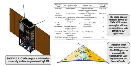
Figure 1. Acquisition geometry of a matrix imager, with HFOV aligned along-track.
Remotesensing 13 02399 g001
Figure 2. 2D representation of HORUS iFOV.
Remotesensing 13 02399 g002
Figure 3. The HORUS camera quadruplet (Types a-b-c-d) FOVs and off-nadir boresight angles (not to scale).
Remotesensing 13 02399 g003
Figure 4. Geometrical relation between view angle and on-board off-nadir boresight angle.
Remotesensing 13 02399 g004
Figure 5. Schematic representation of NASA-JPL MISR view angles, all within the view-angle range reached by HORUS (not to scale).
Remotesensing 13 02399 g005
Figure 6. HORUS CAD model.
Remotesensing 13 02399 g006
Figure 7. Cartesian projections of the HORUS spacecraft CAD model.
Remotesensing 13 02399 g007
Table 1. HORUS main applications and requirements in terms of angle, band, and spatial resolution.
Application TypeView Angle/View AnglesRequired BandAssociated Spatial Resolution
Ocean colorNadir (0 degrees)Blue (main) and green (secondary)/improvements by using NIR275 to 550 m
Surface classificationNadir (0 degrees)red/NIR (main) and green/blue (secondary)275 to 550 m
Land aerosols±60/70.5 degrees (main) and ±45.6/26.1/0 degrees (secondary)Blue and red (main) and green/NIR (secondary)1.1 km
Broadband albedoAllGreen (main) and blue/red/NIR (secondary)1.1 km
Ocean aerosols±60 degrees (main) and ±45.6/26.1/0 degrees (secondary)Red/NIR (main)1.1 km
Cirrus cloud detection±60/70.5 degrees (main) and ±45.6/26.1/0 degrees (secondary)Blue and NIR (main)1.1 km
Cloud heightAll angles (especially stereo images at ±26.1)Red (secondary)1.1 km
Table 2. Off-nadir angles corresponding to the view angle of 70.5° at various orbital heights.
Orbital Height300 km400 km500 km600 km700 km
Boresight   angle   for   σ = 70.5 ° 64.2°62.560.959.558.1
Table 3. Main features of the selected CMOS sensor for HORUS payload.
ParameterValue
Pixel size5.5 µm (H) × 5.5 µm (V)
Resolution4 MP, 2048 × 2048 px
Maximum frame rate90 fps
Shutter typeGlobal
Power consumption (typical)3.2 W
Table 4. Main features of the selected optics for HORUS payload.
ParameterValue
Focal length18.7 mm
F#1.4
Effective aperture diameter13.7 mm
HFOV (along-track)33.4 degrees
VFOV (cross-track)33.4 degrees
Table 5. Main features of the selected COTS filters for HORUS payload.
Spectral BandCentral Wavelength (nm)Spectral Bandwidth
Blue 44330
Green55520
Dark red67020
NIR86560
Table 6. Main features of the HORUS payload module.
Type of CameraHFOV (degrees)VFOV (degrees)Optical Axis Boresight Angle (degrees)Filter’s Central Wavelength (nm)
a33.433.4+50.11. a1: 443 (blue)
2. a2: 555 (green)
3. a3: 670 (red)
4. a4: 865 (NIR)
b33.433.4+16.71. b1: 443 (blue)
2. b2: 555 (green)
3. b3: 670 (red)
4. b4: 865 (NIR)
c33.433.4−16.75. b1: 443 (blue)
6. b2: 555 (green)
7. b3: 670 (red)
8. b4: 865 (NIR)
d33.433.4−50.11. c1: 4430 (blue)
2. c2: 555 (green)
3. c3: 670 (red)
4. c4: 865 (NIR)
Table 7. Ground sample distance (GSD) and diffraction limited resolution at different wavelengths and view angles for 500 km orbital height.
View-Angle (degrees)Type of FilterCentral Wavelength (nm)GSD (m)Diffraction-Limited Resolution (m)
0Dark red443147.1 62.1
Green555147.150.7
Blue670147.145.2
NIR865147.179.0
±26.1Dark red443180.876.4
Green555180.862.3
Blue670180.855.6
NIR865180.897.1
±45.6Dark red443289.8122.4
Green555289.899.9
Blue670289.889.1
NIR865289.8155.7
±60Dark red443534.7226.0
Green555534.7184.4
Blue670534.7164.5
NIR865534.7287.4
±70.5Dark red4431065.8450.9
Green5551065.8368.0
Blue6701065.8328.2
NIR8651065.8573.6
Table 8. SNR analysis parameters.
ParameterValue
Integration time17 ms (60 FPS)
Quantum efficiency50% blue and NIR/60% red and green
Dark current 125e/s
Read noise5e RMS
Full well capacity~106 e
Table 9. SNR analysis results.
0° Nadir26.1°45.6°60°70.5°
Red203191169141116
Green177167148123101
Blue15014212510586
NIR305288254213174
Table 10. HORUS nano-satellite indicative mass budget.
SubsystemMass (kg)MarginMass with Margin (kg)
Structures and mechanisms1.70010%1.870
OBDH0.2005%0.210
EPS2.30010%2.530
TT&C0.6005%0.63
ADCS1.30010%1.430
ODCS1.00010%1.100
Payload optical systems1.40010%1.540
Payload data handling systems0.20010%0.220
Harness0.40020%0.480
Total9.100 10.010
Table 11. Power budget for average daily power consumption.
ComponentPeak Power (W)Duty CycleAverage Power (W)
Solar panels’ generation75.40.4433.20
Main OBDH−0.91−0.90
TT&C on board UHF transmitter−3.00.01−0.03
TT&C on board UHF receiver−0.41−0.40
X-Band transmitter−28.50.08−2.30
ADCS + GPS−4.01−4.00
Thruster−40.00.006−0.24
HORUS camera system−51.20.45−23.04
Image acquisition system−2.00.45−0.90
Margin 2.11
Table 12. Downlink link budgets (UHF and X-band).
UHF (435 MHz)X-Band (8.0 GHz)
ParameterValue (Linear)Value (dB)Value (Linear)Value (dB)
RF output (spacecraft)1 W0 dBW34.77 dBW
Spacecraft line loss 0.6 dB 0.6 dB
Spacecraft antenna gain (and pointing losses) −0.5 dB 13 dB
Free space loss5 degrees elevation151.6 dB5 degrees elevation176.9 dB
Ionospheric/Atmospheric losses 2.5 dB 2.4 dB
Polarization losses 3 dB 1 dB
Ground station antenna pointing loss 0.7 dB 1.1 dB
Ground station antenna gain 14.1 dBi 48.3 dBi
Effective noise temperature510 K27.08 dBK245.36 K23.90 dBK
Ground station line losses 1 dB 1 dB
Data rate9600 bps39.8 dBHz300 Mbps80.0 dBHz
Eb/N0 17.7 dB 6.77 dB
Eb/N0 threshold(GMSK, BER 10−5)10.6 dBBand efficient 8PSK Concatenated Viterbi/Reed Solomon Rate 1/24.2 dB
Link margin 5.2 dB 3.57 dB
Table 13. Data amount generated in one single acquisition in one observation angle.
ParameterValue
Pixels per line2048
Bits per pixels12
Bits per pixel-line24,576
Orbit altitude (km)500
Orbital speed (km/s)7.616
Ground speed (km/s)7.062
Ground speed (pixel/s)48.04
Required frame rate with 25% margin (fps)60
Payload reference duty cycle0.45
Average generated data bit rate (Mbps)0.664
Total data amount per day (Gbits)57.331
Data rate of the transmission system (Mbps)300
Daily transmission time per observation angle, per spectral band (50% lossless data compression)1 min 36 s
Table 14. Daily data and downlink time for “MISR-like” observation plan.
Total data amount per day, including nine angles and four spectral bands (Gbits)2064
Daily transmission time per observation angle, per spectral band
(50% lossless data compression)
57 min 20 s
Publisher’s Note: MDPI stays neutral with regard to jurisdictional claims in published maps and institutional affiliations.

