
Estimation of Forest LAI Using Discrete Airborne LiDAR: A Review


1
State Key Laboratory of Remote Sensing Science, Jointly Sponsored by Beijing Normal University and Institute of Remote Sensing and Digital Earth of Chinese Academy of Sciences, Beijing 100875, China
2
Beijing Engineering Research Center for Global Land Remote Sensing Products, Institute of Remote Sensing Science and Engineering, Faculty of Geographical Science, Beijing Normal University, Beijing 100875, China
3
State Forestry and Grassland Administration Key Laboratory of Forest Resources and Environmental Management, Beijing Forestry University, Beijing 100875, China
*
Author to whom correspondence should be addressed.
Remote Sens. 2021, 13(12), 2408; https://0-doi-org.brum.beds.ac.uk/10.3390/rs13122408
Submission received: 5 May 2021
/
Revised: 7 June 2021
/
Accepted: 15 June 2021
/
Published: 19 June 2021
Abstract
:The leaf area index (LAI) is an essential input parameter for quantitatively studying the energy and mass balance in soil-vegetation-atmosphere transfer systems. As an active remote sensing technology, light detection and ranging (LiDAR) provides a new method to describe forest canopy LAI. This paper reviewed the primary LAI retrieval methods using point cloud data (PCD) obtained by discrete airborne LiDAR scanner (DALS), its validation scheme, and its limitations. There are two types of LAI retrieval methods based on DALS PCD, i.e., the empirical regression and the gap fraction (GF) model. In the empirical model, tree height-related variables, LiDAR penetration indexes (LPIs), and canopy cover are the most widely used proxy variables. The height-related proxies are used most frequently; however, the LPIs proved the most efficient proxy. The GF model based on the Beer-Lambert law has been proven useful to estimate LAI; however, the suitability of LPIs is site-, tree species-, and LiDAR system-dependent. In the local validation in previous studies, poor scalability of both empirical and GF models in time, space, and across different DALS systems was observed, which means that field measurements are still needed to calibrate both types of models. The method to correct the impact from the clumping effect and woody material using DALS PCD and the saturation effect for both empirical and GF models still needs further exploration. Of most importance, further work is desired to emphasize assessing the transferability of published methods to new geographic contexts, different DALS sensors, and survey characteristics, based on figuring out the influence of each factor on the LAI retrieval process using DALS PCD. In addition, from a methodological perspective, taking advantage of DALS PCD in characterizing the 3D structure of the canopy, making full use of the ability of machine learning methods in the fusion of multisource data, developing a spatiotemporal scalable model of canopy structure parameters including LAI, and using multisource and heterogeneous data are promising areas of research.

1. Introduction
The leaf area index (LAI) is a critical indicator of vegetation status. It is widely used in many fields, such as earth science, agronomy, ecology, and forestry [1], as an essential input variable to the land surface process model [2,3]. LAI is a dimensionless variable (or m2/m2), and its concept has progressed through a long process of definition and clarification [4,5,6,7]. In quantitative remote sensing, the most popular and widely accepted definition of LAI refers to half of the total leaf area per unit ground area [6].
Direct or indirect measurements on the ground and remote sensing inversion from remotely sensed data are the primary methods used to determine LAI. Direct measurement methods consist of destructive sampling, litterfall collection [8], and point quadrat sampling [9,10,11]. The indirect methods employ non-contact optical equipment to measure the canopy gap fraction (GF), i.e., the physical GF [12], e.g., by LAI-2200C, or geometric GF [13], e.g., by digital hemisphere photo (DHP), and estimate the canopy LAI using the Beer-Lambert law. More details of these indirect methods can be found in the recent review by Yan [14]. However, both ground-based direct and indirect measurements are laborious, even with the new generation Internet of Things-based equipment, e.g., LAINet [15], and may be infeasible due to spatial accessibility.
Remote sensing is the only feasible method to retrieve LAI on a large or even global scale [16]. Several global LAI products have been made publicly available in the last decade based on passive remote imagery, e.g., MODIS-LAI [17], GLOBCARBON-LAI [18], and CYCLOPES-LAI [19]. However, such a passive remote sensing-based LAI may suffer from spectral saturation and poor atmospheric conditions [20,21]. Moreover, it can only capture horizontally distributed features of the canopy in a fixed spatial resolution depending on the specific sensor [22]. In addition to passive remote, a type of active remote sensing sensor, light detection and ranging (LiDAR) has been increasingly used for LAI estimation [20,23,24,25]. Because of its ability to penetrate the canopy, LiDAR has been proven to mitigate signal saturation to some extent [26,27]. In addition, LiDAR can simultaneously characterize the horizontal and vertical structure of canopy [28,29] at multiple spatial scales, such as individual trees, sample plots, or areas [30]. Furthermore, as a technique that is essentially different from passive remote sensing, LiDAR-derived LAI provides a new independent source for assessing the LAI retrieval model based on passive remote sensing [31,32,33,34].
Different LiDAR systems, e.g., full-waveform [35] and discrete LiDAR systems [20], have been employed for LAI retrieval. The proposed methods for different types of LiDAR systems have been comprehensively reviewed recently by Wang from a more framework-oriented view [36]. However, to our knowledge, there is still a lack of a more specific review aiming at the LAI retrieval methods for discrete airborne LiDAR scanners (DALS) which is one of the most popular types of LiDAR systems in forest resource surveys [37,38,39]. Since the commercialization of DALS LiDAR systems at the beginning of this century, point cloud data (PCD) obtained by DALS has been widely used to estimate LAI [20,23,25,27,39,40,41,42,43,44]. However, published literature has shown that the accuracy of LAI inversion based on DALS PCD (typically, RMSE > 0.5 [25]) can barely meet the requirements of the global climate change research community (GCOS) who demands the inversion accuracy of LAI to be 0.5 LAI units [45]. The gap between the accuracy of LiDAR LAI products and application requirements requires an in-depth understanding of LAI estimation methods based on DALS PCD. We believe that this topic must be investigated to guide selecting an optimal method from various candidate methods when conducting LAI estimation using DALS PCD. In this context, this paper expects to provide a review of the LAI retrieval methods using DALS PCD, the validation scheme and limitations of those methods, and future development trends in this field.
2. An Overview of the DALS System
The basic principle of different LiDAR systems is similar: LiDAR scanner emits a pulse and measures the distance between the sensor and ground object. The distance, subsequently, is converted into the geographic coordinates of the object, combining with GPS and IMU (Inertial Measurement Unit) mounted onto the platform together with the LiDAR scanner. Current LiDAR systems can be categorized as spaceborne laser scanning (SLS), airborne laser scanning (ALS), terrestrial laser scanning (TLS), mobile (mobile laser scanning, MLS) and unmanned aerial vehicle (UAV) laser scanning (ULS) based on platforms [46] or as discrete, full-waveform and photon-counting LiDAR based on their sampling frequencies [42]. More details of these types of LiDAR systems can be found in [46].
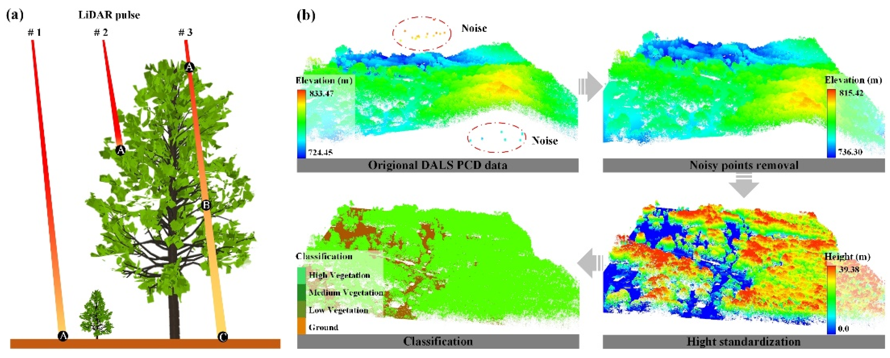
For discrete airborne laser scanners (DALS), the size of the footprint is small (typically < 1 m [46]). The LiDAR beam can penetrate the canopy through the gaps in the canopy, which is accompanied by the expanding of the footprint and the attenuation of the pulse energy as illustrated in Figure 1a. In Figure 1a, the width of the path represents the gradually expanding footprint, and the gradient fill of the path represents the attenuation of pulse with the propagation of beam in the canopy. Along with the propagation of pulse in the canopy, multi-return from objects in the path of the pulse can be recorded (typically < 7 for DALS [42]) until the pulse is entirely occluded by the canopy component (e.g., # 2A in Figure 1a) or finally reaches the ground (e.g., # 3C in Figure 1a) [47]. In addition to the geographic coordinates of each return, PCD in LAS format [48] also records information such as the number of returns (NRs), return number (RN), and intensity of each return, etc.
A set of preprocessing of DALS PCD is required before further analysis, including noisy point removal, point cloud filtering, height standardization, and classification (Figure 1b). These 3D points in DALS PCD can be classified according to NRs and RN relationships (Table 1). Combined with the land coverage type represented by the point, e.g., the ground or vegetation, these points can further be classified into single ground echo (), single vegetation echo (), first vegetation echo (), and last ground echo (), etc.
3. LAI Retrieval Methods Using DALS PCD
3.1. Physical Method
The Beer-Lambert (BL) law relates the attenuation of light to the material properties through which the light travels [49]. The gap fraction model derived from the BL law can be used to describe the relationship between LAI and the gap fraction (GF) of the canopy as follows [12]:
where is the gap fraction at the view zenith angle , is the mean inclination angle of canopy component, and is the Ross Nilson G-function, which refers to the fraction of a unit plant area projected onto a plane perpendicular to a direction making an angle with nadir [50]. From Equation (1), the LAI can be expressed as:
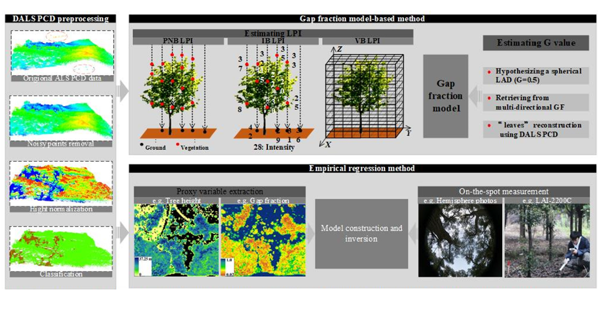
and in Equation (2) can both be estimated by DALS PCD. The generally characterized by the LiDAR penetration indexes (LPIs) derived from DALS PCD. Existing LPIs can be summarized into three types, i.e., point-number-based LPIs (PNB LPIs), point-intensity-based LPIs (IB LPIs), and voxel-based LPIs (VB LPIs) (see Section 3.1.1). Three types of methods have been proposed to estimate the of canopy (see Section 3.1.2). The process of estimating LAI basing on the GF model is straightforward when LPIs and are available (Figure 2).
3.1.1. Estimating LPIs from DALS PCD
As aforementioned, there are three types of LPIs: (1) Point-number-based LPIs (PNB LPIs), where the LPI is calculated as the ratio of the number of point clouds classified as the ground to the total amount of points; (2) Point-intensity-based LPIs (IB LPIs), where IB LPIs is calculated as the ratio of the intensity of ground points to the total intensity; and (3) Voxel-based LPIs (VB LPIs), which divides the space occupied by PCD into 3D voxels cell by subjectively selecting the sizes of , , and , and the corresponding LPIs is calculated as the ratio of empty voxels that do not contain point clouds to the total voxels [23]. An example of such three types of LPIs is presented in Figure 2. There are more than ten forms of LPIs, and some widely used are listed in Table 2.
Previous studies have shown that different LPIs are highly correlated but may exhibit a significant absolute difference from each other [21]. However, the proper form of the LPIs metric is currently unclear, and researchers typically subjectively choose an LPIs form for specific regions, times, tree species, and data characteristics [33]. However, there is some consensus about existing LPIs forms (Table 2):
- For PNB LPIs, the , derived from the single return, typically underestimates GF due to the lack of sensitivity of a single echo to the small gap within the crown [41,47,55,56], resulting in 20–30% overestimation of LAI [51]. Conversely, , which is calculated by single and last return, typically overestimates GF, thus underestimates LAI [33,55]. Weighted LPIs (e.g., , ) are typically plagued with the suitability of the weights for different return types [20,57]. Voxel-based LPIs, however, may be biased due to a wrong cell size selected subjectively [23,36,58].
- For IB LPIs, the reflectance of background and vegetation is an important factor that affects the energy from either the background or vegetation [40,59]. Therefore, it is necessary to calibrate IB LPIs for better performance [41,47,60] by introducing the backscattering coefficient of background and vegetation, or at least their ratio ().
Given the fact that spectral property of background and vegetation not only affects the reflected energy but also the number of returns from either the background or vegetation and thus in further PNB LPIs, a similar to IB LPIs calibration method was proposed aiming at PNB LPIs in [25]:
where is the adjusted PNB LPIs. The can be derived from ground measured spectral data [61], remotely sensed hyperspectral data [25], or the intensity of returns [42,62]. However, the estimation of still needs further study (see Section 5.2).
3.1.2. Estimating G from DALS PCD
The G function in Equation (2) is a function of the observation zenith angle and leaf orientation [63,64]. For most tree species, the leaf is nearly uniformly distributed in the azimuth direction [65]; therefore, leaf orientation typically refers to the leaf angular distribution (LAD) in the zenith direction [66]. The G function can be expressed in terms of LAD and observation zenith angle as:
where is the Reeve kernel, i.e., the average projection of unit area of the leaf, of angle and uniform azimuth, in the direction of the probe [9,67]. is the LAD of the canopy.
It was almost impossible to directly measure the LAD of the forest canopy with the conventional methods [12,68] due to the forest canopy being tall and intricate [12]. To quantitatively describe the LAD of a canopy, many theoretical models have been proposed, such as the spherical [69], ellipsoidal [64], and beta function models [70]. The G of the canopy that satisfies the spherical model is independent of the observation direction and always equals 0.5 [47,69,71]. Studies on these theoretical LAD models also found that G is approximately equal to 0.5 when the observation zenith angle is approximately 57.3°, regardless of the LAD [67,72].
Another way to obtain the G function is based on multi-directional GF [12,73]. However, only a few observation angles are available in a small area (e.g., plot), particularly when the platform height was increased to save data acquisition costs [23]. Considering that LAD is relatively stable in a given area compared to the variation in LAI [40], Qu et al. hypothesized that LAD in a larger area that is above the plot, called “tile,” can be described by an ellipsoidal model [64] with parameters that were estimated using the nonlinear optimization method [25].
LAD has been successfully extracted from PCD acquired by terrestrial laser scanning (TLS) directly. TLS typically has a smaller footprint (<5 cm) and footprint space interval (<5 cm) [46] and hence a higher point density compared with DALS. Under the assumption that the points in PCD can characterize the leaf’s surface, a certain number of nearby points called the “support region” were reconstructed as “leaves.” Consequently, the angle between the normal vector of “leaves” and zenith direction was calculated as leaf inclination angle [74,75]. Zheng et al. tried to apply this method to DALS PCD (point density > 20 pts/m2) [23]. Ma et al. also applied the method to DALS PCD to obtain the leaf orientation distribution of the inclinational and azimuthal angles simultaneously [71]. The “occlusion effect,” i.e., the upper canopy element, blocks some of the LiDAR pulses completely (Figure 1) and prevents it from sampling behind upper elements [41,76], but would less limit the application of this method because measuring some samples is enough to represent the LAD of the whole canopy [14]. While the pulse footprint size (>10 cm) and the footprint space interval (>20 cm) [46] of the DALS system is generally larger than the leaf characteristic size, a study has proved that the canopy extinction coefficient (i.e., in Equation (1)) extracted from DALS PCD can also effectively characterize the canopy in some specific view zenith angles [71].
In summary, there are four types of methods to determine the G of a canopy, i.e., the LAD- and observation-direction-independent method (a spherical model), LAD-independent hinge zenith angle (57.3°), multi-directional GF-based method, and “leaves” reconstruction method based on LiDAR PCD. However, studies have shown that LAD is strongly dependent on tree species, age [20], and even time [63,77], which implies that a spherical model may not suitable in some cases. Existing LiDAR systems designed to obtain an accurate digital elevation model work on a small scan angle (typically < 30°), far away from the hinge observation angle. Moreover, the details of the multi-directional GF-based method still require further verification, such as the size of “tile” and prior knowledge about the constraints on model parameters, and its identical LAD assumption may not be suitable for mixed forest sites. The “leaves” reconstruction method seems a promising one, especially with the DALS increasingly equipped with a higher pulse repetition frequency which theoretically enhances the ability of DALS to sample canopy elements in more detail [78]. Apart from the LAD-independent hinge zenith angle method, the other three methods can be employed for G estimation using DALS PCD (Figure 2).
3.2. Empirical Regression Based on Proxy Variables
Empirical models are based on the allometric growth equation model, which assumes that the target canopy structure parameters (e.g., LAI) are related to other canopy structure parameters (e.g., tree height, crown width, etc.) [79]. The proxies assessed in previous studies are mainly constructed based on some heuristic clues and can be categorized into three types, i.e., height-related variables, cover-related, and LPIs (Table 3). A high correlation was found between LPIs [44], cover related metrics [60], and LAI; however, these models constructed based on the number/intensity of different types of returns are difficult to expand between different LiDAR systems even in the same region [21]. The height-related proxies were used frequently; however, a relatively lower correlation was found between such a proxy and LAI [60,80,81] compared with LPIs. The empirical method was also highly sensitive to tree age, time, stand density, the accuracy of field measurement data of LAI, etc. [53,55,57,82]. Overall, all regression models are calibrated and validated against local field data; however, reliable models that can be transferred to other locations, times, and different LiDAR systems are unfortunately lacking [21,53].
4. The Validation of DALS PCD-Based LAI
Fang summarized six types of schemes for remote sensing product/algorithm validation [2]. These schemes also outline the process of DALS PCD-based LAI validation, such as field-to-remote sensing direct comparison, validation with model-simulated LAI, and the inter-comparison of multiple LAI products, etc.
The field-to-DALS LAI direct comparison is involuntary, as the DALS can characterize the canopy at a plot scale corresponding with that of ground direct/indirect measurement. The indirect measurement of LAI using LAI-2200 and DHP is the most used data source for DALS PCD-based LAI validation, and a strong correlation was reported [20,77]. There were three problems when such an indirect field measurement was used to validate the PCD ALS-LAI. Firstly, the conical field of view of field measure devices (CFOV) mismatch with the pre-defined field plot size used to extract the PCD subset of field plot (SPCD). The CFOV is generally larger than the pre-defined field plot size, and hence a SPCD that is comparable to the tree height within the plot or a larger one than pre-set plot size is recommended to construct the LAI retrieval model according to the results of previous studies [20,33,39]; Secondly, the inherent difference between DALS and ground measurement devices in characterizing the canopy results in different data representations of the same forest canopies [57,87]. The DALS capture more foliage elements in the upper canopy, while more stems and lower canopy components will be sampled by field indirect measurement devices [43], even compared with the TLS that follows the identical physical basis but different observation configuration [71]. Finally, the quality of the field measurement would distort the process of validation. For example, Zhao tested the uncertainties of field LAI measurement using DHP caused by the analysts or algorithms and found such uncertainties were in the same order of magnitude as or even larger than that of the fitted regression models [33].
On the contrary, radiative transfer models (RTMs), such as FLIGHT [88] and DART [89], etc., are capable of simulating LiDAR data with a controlled canopy parameter, which can exclude the influences from field reference data. Based on the simulated DALS PCD using the DART model, Yin assessed the LAI retrieval model constructed by different LPIs and pointed out that the models based on IB LPIs showed higher accuracy and reliability than PNB LPIs [53]. However, the effectiveness of such a RTMs-based validation is restricted by the fineness of canopy reconstruction [87] and the parameters of the DALS system that is not always available for commercial DALS sensors [90].
The inter-comparison method assesses the temporal and spatial consistency of remote sensing products, which is an important aspect of validation [2,36]. The inter-comparison between the DALS PCD-based LAI and the satellite LAI products, e.g., GLOBCARBON LAI [33], and MODIS LAI [31], suggests that the DALS PCD-based LAI can serve as a reliable reference for validating moderate-resolution LAI products. The misregistration between the DALS PCD and the satellite could severely impact the pixel-wise inter-comparison. The consistency between DALS-LAI and GLOBCARBON-LAI was significantly improved with a correlation coefficient from 0.08 to 0.85 for pine when the misregistration was corrected [33].
As summarized by Wang, LiDAR-based LAI validation was performed at a limited local scale [36], partly due to the poor transferability of the proposed model (see Section 5.1) and the high acquisition cost of DALS PCD. More comprehensive validation is required, namely, but not limited to, across different forests [21] to enhance understanding of and further improve the LAI retrieval models based on DALS PCD.
5. Challenges of Estimation of Forest LAI Based on DALS PCD
5.1. Model Scalability
The greatest problem with using DALS PCD to estimate LAI is the poor scalability of the model in time, space, and across different DALS systems. Currently, both empirical regression and the physical GF model rely on field data to construct or calibrate model fraught with inaccuracy [43], which reveals that DALS PCD-based LAI retrieval is unreliable for application without calibration by field measurement.
Such a poor transferability of the model has been widely recognized and was ascribed to the LiDAR system (e.g., pulse repetition frequency (PRF), pulse energy, beam divergence, etc.), observation geometry (e.g., platform height, scanning angle, etc.), properties of the ground object (e.g., spatial distribution, moisture content, spectral characteristics, etc.) and hypsography (e.g., slope, relative slope with the incident pulse, etc.). These factors jointly determine the PCD characteristics, such as the size of the footprint, point density, spatial distribution of point and data volume, etc., and also determine the applicable situations to which DALS PCD can be used effectively [46]. Efforts have been paid on the influences from part of these factors on LAI retrieval based on DALS PCD, such as the characteristics of the LiDAR system, namely the scan angle [91], point density [92], sensor altitude [93], etc. Nevertheless, few studies have investigated the properties of the canopy (e.g., spectral characteristics, spatial heterogeneity) and the relationships between various factors, which is necessary for the effective acquisition, autoprocessing, and accurate application of ALS data.
Overall, the disparity reported by the current literature regarding the estimation of LAI from DALS PCD highlights the necessity to figure out the influence of the aforementioned factors. On this basis, more robust models which can be transferred from one case to other are required to fill the gap between the experiment and practical application [21].
5.2. Calibration of LPIs with a Target Spectral Property
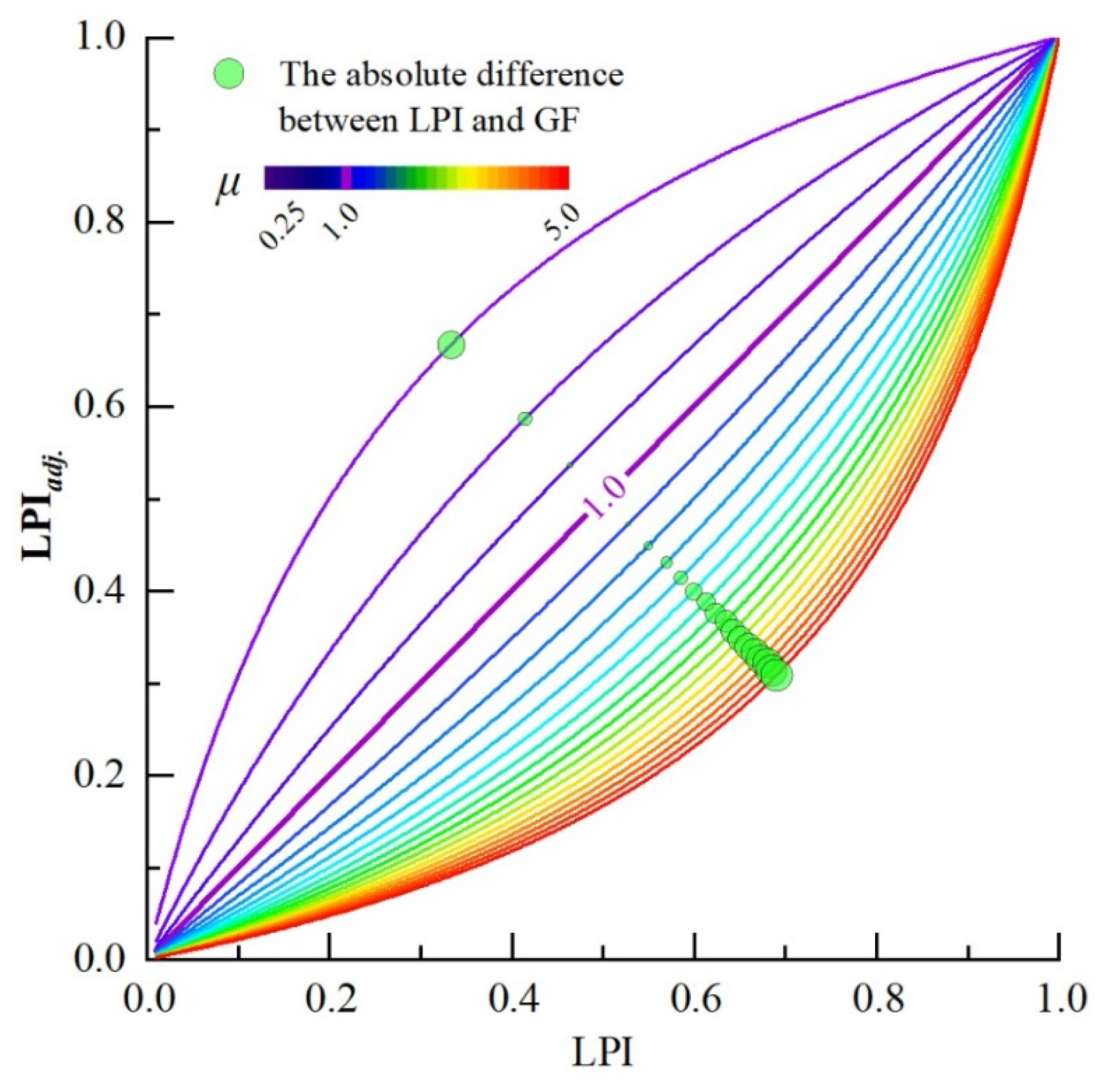
Equation (3) shows that the spectral properties of background and vegetation are important factors that can lead to the deviation of LPIs from GF. The discrepancy between LPIs and GF caused by spectral properties will increase rapidly when the spectral difference of the background and vegetation increases, particularly with medium canopy cover (Figure 3). With obtained by Solberg [41], the overestimation of LPIs to GF can reach 79.8% (Equation (3)) if the spectral difference is ignored (i.e., ).
Three methods can be used to determine μ: (1) calculating μ using ground-based spectral data [47,61] or remotely sensed hyperspectral data [25]; (2) determining μ using a series of trials in a given range (e.g., μ = 1 to 10) and selecting μ that produces the highest coefficient of determination R2 in a linear regression between retrieval LAI and ground-based measured LAI [41]; and (3) calculating μ using return intensities [42,62,94]. The first two methods require additional ground-based measurements in addition to LiDAR data and thus require more effort to collect auxiliary data, i.e., spectral or LAI data, that are consistent with the LiDAR data in both time and space. If no field spectral data are available, field spectral data collected in the historical database can be used as a reference [61,95]. However, the term “ground” in LiDAR data does not mean “soil” because the classifying threshold of LiDAR to differentiate vegetation and ground is a standardized height [94], which indicates that all points below the given threshold are classified as a ground [96]. This discrepancy partly explains the relatively low correlation of the LiDAR intensity with the field-measured spectrum [97]. It indicates that there is significant uncertainty in using the μ calculated from the field spectral or hyperspectral data for the LPIs correction directly. The third method using returns’ intensity from vegetation and ground to calibrate LPIs, cannot accurately separate spectrally independent quantities from return intensities [98,99]. One reason for these difficulties is that the LiDAR manufacturers do not release all LiDAR system parameters, e.g., the intensity quantification algorithm, to end-users due to confidential considerations [21,100]. The missing DALS system parameters limit the radiation correction of point cloud intensity [1,54,101,102], indicating that the methods extracting μ directly from the intensity of returns must be validated.
5.3. Correcting Impact from the Clumping Effect and Woody Material
Clumping and woody materials are the most important factors estimating true LAI in indirect ground measurements and remote sensing [103,104]. The former may lead to a 30–70% underestimation of LAI [105], and the latter may lead to a 7–40% overestimation of LAI [106].
Clumping can simultaneously result from within- and between-crown and the shape of the crown. Many efforts have been exerted to correct the clumping effect. Proposed methods include, as systematical reviewed by Yan [66], the finite-length averaging method (LX) [107], gap-size distribution method (CC) [105], method combining the two methods above (CLX) [108], and path length distribution method (PATH) [109]. Some of these approaches have been successfully applied to DALS PCD data by transforming 3D data into 2D imagery data, considering the low point density due to the occlusion effect and low sampling density. Mariano had assessed the performance of CC on DALS PCD, and the results indicate that the clumping index of CC showed good agreement with that from DHP (, ) [110]. The PATH model has been used for both DALS PCD and TLS PCD, which inherently contains the path length and distribution that the PATH model requires [32,111]. In addition, given that the LiDAR pulse can reasonably be regarded as a systematic sampling of the canopy [32], some statistical methods have also been introduced to estimate clumping index, such as standardized Morisita’s index (SMI) [112] and Pielou coefficient of segregation (PCS) [113], indexes widely used in ecological studies to describe the distribution of species. By voxelating the PCD from TLS and DALS and classifying the voxel into different species (i.e., empty or vegetation voxel), Mariano investigated the SMI and PCS on estimating clumping index, and the results showed that the performance of both indexes depends on the size of the voxel [110].
The woody component is another important factor that causes retrieval LAI based on the GF model to deviate from the true LAI. From the spectral perspective, although the intensity of LiDAR returns can be used to identify vegetation types [114,115], it is not easy to distinguish different canopy components using a single band. From the spatial side, the advantage of LiDAR in describes the geometrical characters of the canopy component would be a promising direction to classify out the woody component, however, which is restricted by the size of the footprint and PRF of the existing ALS system [71]. Nevertheless, there is still hope: (1) the multiband LiDAR system was invented long ago [116] and has been commercialized in recent years [117,118], making it possible to identify woody components [77]; (2) with the development of the ALS system and the combination of TLS and ALS [36], the footprint is getting smaller, and the PRF is getting higher increasingly [119]. Therefore, the canopy component identification method developed from TLS PCD [120,121] will be reasonably applicable to ALS PCD to eliminate contribution from woody elements.
5.4. Saturation Effect
Although a LiDAR pulse can penetrate a forest canopy to some extent, ALS PCD-based LAI may saturate in some cases. For GF model-based method, the saturation refers to the cases that the pulse cannot penetrate the complete canopy, i.e., a lack of ground return, resulting in a gap rate of 0, which leads to failure of the LAI determination based on the gap fraction model (Equation (2)) [21,51]. For the empirical regression model, the saturation is similar to that of passive remote sensing: the retrieval LAI does not increase with proxies, i.e., vegetation indexes for passive remote sensing or LiDAR metric for LiDAR, when the proxies exceed a certain value [33].
As far as we know, there is no study aiming at the saturation effect of LAI retrieval based on DALS PCD due to the well-known fact that the LiDAR beam does have penetration ability. By summarizing published literature, some of the critical LAI of saturation are listed in Table 4. In passive remote sensing, many researchers have observed that optically-derived vegetation indexes tend to saturation when LAI values are greater than 3 [24,122]. In contrast, LiDAR-based LAI retrieval does have, as expected, a larger critical saturation value of LAI ( from Table 4); however, it seems condition-dependent, including upon tree species, model type, and LiDAR system used, etc. Interestingly, the point density (or pulse density) does not appear to be, as expected, a critical factor to the saturation effect. Unfortunately, it is hard to draw definite conclusions based on the limited samples we have.
For the GF model-based method, studies have proposed several solutions for saturation, including the method of increasing pulse density using a larger PRF, the method of substituting the infinitesimal nonzero value for zero-gap, the method of increasing the spatial extent to gain a certain amount of ground return, and the method of configuring the LIDAR instrument to be more sensitive to returns with low energy [77]. However, each method has advantages and disadvantages. For example, increasing the spatial extent will cause a lower spatial resolution of the results [56] and difficulty in model verification. Furthermore, higher sensor sensitivity is bound to increase data noise, which complicates data processing.
For the empirical regression model, it seems that a combination of the metrics constructed by geometrical- and intensity-related variable can delay the saturation effect to some extent [60], which can partly ascribe to the increased information from different sources. However, the contribution from more metrics may be limited; a study by Tesfamichael showed that the model constructed by thirteen metrics had ignorable improvement compared with the three-metrics model [123].
6. Conclusions and Future Direction
As a critical parameter of a forest canopy structure, LAI can be quickly determined at multi-spatial scales using a discrete ALS LiDAR system widely used in forestry investigations. In this review, the methods and existing problems of LAI inversion based on DALS PCD are systematically summarized.
The empirical regression method and gap fraction models are the two dominant methods used to determine LAI using DALS PCD. Tree height and its derivative variables (e.g., percentiles of tree height), LPIs, and canopy cover are widely used proxy variables for empirical regression model construction. The gap fraction model estimates LAI using Beer-Lambert’s law using LPIs derived from ALS PCD. The most significant problem with LAI retrieval using DALS PCD, for both empirical regression methods and gap fraction model, is the poor scalability of the model in time, space, and across different DALS systems. Further work is desired to emphasize assessing the transferability of published methods to new geographic contexts, sensor types, and survey characteristics, based on figuring out the influence of each factor on the LAI retrieval process using DALS PCD.
Unlike passive remote sensing that records an integrated signal from reflected energy, LiDAR provides a chance to characterize the canopy in high detail in a vertical direction [21]. Moreover, LiDAR also provides a new avenue for correcting the impacts of the clumping effect and woody material. For example, developing a multiband LiDAR system will make it possible to distinguish woody components in the canopy from a spectral perspective. Additionally, an increasingly smaller footprint and larger PRF will provide more effective data to construct canopy 3D structures accurately and determine the LAD needed for a reliable LAI retrieval [78].
From a methodological point of view, with the development of remote sensing technology, LAI estimation has entered a stage of integrating multisource data [29]. Compared to traditional methods, machine learning algorithms (e.g., neural networks) can fuse more auxiliary information [126], such as spectrum-related data from passive remote sensors and multisource historical data, and have been widely used in the inversion of canopy structure parameters such as LAI [127,128]. However, the training features set from traditional remote sensing methods are primarily composed of the spectrum, spectral index (e.g., NDVI), and 2D spatial structure information, which typically has strong collinearities [129]. However, LiDAR can provide 3D canopy structure information from a new perspective, theoretically providing a new data source for model training [130]. Therefore, using multisource, multiband, multiplatform, homogeneous, and heterogeneous data and taking advantage of machine learning algorithms to describe the inversion of canopy structure parameters should be investigated in future research [130].
Author Contributions
Conceptualization, L.T. and Y.Q.; writing—original draft preparation, L.T.; writing—review and editing, L.T., Y.Q. and J.Q. All authors have read and agreed to the published version of the manuscript.
Funding
This research was funded by the National Natural Science Foundation of China, grant number 41671333, and National key research and development program of China, grant number 2016YFC0500103.
Acknowledgments
We thank the anonymous reviewers for helpful insights in improving this paper.
Conflicts of Interest
The authors declare no conflict of interest.
References
- Riaño, D.; Valladares, F.; Condés, S.; Chuvieco, E. Estimation of leaf area index and covered ground from airborne laser scanner (Lidar) in two contrasting forests. Agric. For. Meteorol. 2004, 124, 269–275. [Google Scholar] [CrossRef]
- Fang, H.L.; Baret, F.; Plummer, S.; Schaepman-Strub, G. An Overview of Global Leaf Area Index (LAI): Methods, Products, Validation, and Applications. Rev. Geophys. 2019, 57, 739–799. [Google Scholar] [CrossRef]
- GCOS. Systematic Observation Requirements for Satellite-Based Products for Climate Supplemental Details to the Satellite-Based Component of the Implementation Plan for the Global Observing System for Climate in Support of the UNFCCC-2011 Update; Word Meteorological Organization: Geneva, Switzerland, 2011; Available online: https://library.wmo.int/doc_num.php?explnum_id=3710 (accessed on 4 January 2021).
- Watson, D.J. Comparative Physiological Studies on the Growth of Field Crops: I. Variation in Net Assimilation Rate and Leaf Area between Species and Varieties, and within and between Years. Ann. Bot. 1947, 11, 41–76. [Google Scholar] [CrossRef]
- Ross, J. The Radiation Regime and Architecture of Plant Stands; W. Junk.: The Hague, The Netherlands, 1981; ISBN 9061936071. [Google Scholar]
- Black, T.A.; Chen, J.M.; Lee, X.H.; Sagar, R.M. Characteristics of shortwave and longwave irradiances under a Douglas-fir forest stand. Can. J. For. Res. 1991, 21, 1020–1028. [Google Scholar] [CrossRef]
- Chen, J.M.; Black, T.A. Defining leaf area index for non-flat leaves. Plant Cell Env. 1992, 15, 421–429. [Google Scholar] [CrossRef]
- Chen, J.M.; Rich, P.M.; Gower, S.T.; Norman, J.M.; Plummer, S. Leaf area index of boreal forests: Theory, techniques, and measurements. J. Geophys. Res. 1997, 102, 29429–29443. [Google Scholar] [CrossRef]
- Wilson, J.W. Inclined point quadrats. N. Phytol. 1960, 59, 1–7. [Google Scholar] [CrossRef]
- Levy, E.B.; Madden, E.A. The point method of pasture analysis. N. Z. J. Agric. 1933, 46, 267–279. [Google Scholar]
- Caldwell, M.M.; Harris, G.W.; Dzurec, R.S. A fiber optic point quadrat system for improved accuracy in vegetation sampling. Oecologia 1983, 59, 417–418. [Google Scholar] [CrossRef]
- Lang, A.R.G.; Xiang, Y.Q.; Norman, J.M. Crop structure and the penetration of direct sunlight. Agric. For. Meteorol. 1985, 35, 83–101. [Google Scholar] [CrossRef]
- Anderssen, R.; Jackett, D.; Jupp, D.; Norman, J. Interpretation of and simple formulas for some key linear functionals of the foliage angle distribution. Agric. For. Meteorol. 1985, 36, 165–188. [Google Scholar] [CrossRef]
- Yan, G.J.; Hu, R.H.; Luo, J.H.; Weiss, M.; Jiang, H.L.; Mu, X.H.; Xie, D.H.; Zhang, W.M. Review of indirect optical measurements of leaf area index: Recent advances, challenges, and perspectives. Agric. For. Meteorol. 2019, 265, 390–411. [Google Scholar] [CrossRef]
- Yu, L.; Shang, J.; Cheng, Z.; Gao, Z.; Wang, Z.; Tian, L.; Wang, D.; Che, T.; Jin, R.; Liu, J.; et al. Assessment of Cornfield LAI Retrieved from Multi-Source Satellite Data Using Continuous Field LAI Measurements Based on a Wireless Sensor Network. Remote Sens. 2020, 12, 3304. [Google Scholar] [CrossRef]
- White, M.A.; Asner, G.P.; Nemani, R.R.; Privette, J.L.; Running, S.W. Measuring Fractional Cover and Leaf Area Index in Arid Ecosystems. Remote Sens. Environ. 2000, 74, 45–57. [Google Scholar] [CrossRef]
- Knyazikhin, Y.; Glassy, J.; Privette, J.; Tian, Y.; Lotsch, A.; Zhang, Y.; Wang, Y.; Morisette, J.; Votava, P.; Myneni, R.; et al. MODIS Leaf Area Index (LAI) and Fraction of Photosynthetically Active Radiation Absorbed by Vegetation (FPAR) Product (MOD15) Algorithm Theoretical Basis Document. Available online: http://modis.gsfc.nasa.gov/data/atbd/atbd_mod15.pdf (accessed on 10 April 2021).
- Deng, F.; Chen, J.M.; Plummer, S.; Chen, M.Z.; Pisek, J. Algorithm for global leaf area index retrieval using satellite imagery. IEEE Trans. Geosci. Remote Sens. 2006, 44, 2219–2229. [Google Scholar] [CrossRef] [Green Version]
- Baret, F.; Hagolle, O.; Geiger, B.; Bicheron, P.; Miras, B.; Huc, M.; Berthelot, B.; Niño, F.; Weiss, M.; Samain, O.; et al. LAI, fAPAR and fCover CYCLOPES global products derived from VEGETATION. Remote Sens. Environ. 2007, 110, 275–286. [Google Scholar] [CrossRef] [Green Version]
- Solberg, S.; Brunner, A.; Hanssen, K.H.; Lange, H.; Næsset, E.; Rautiainen, M.; Stenberg, P. Mapping LAI in a Norway spruce forest using airborne lase r scanning. Remote Sens. Environ. 2009, 113, 2317–2327. [Google Scholar] [CrossRef]
- Sumnall, M.; Peduzzi, A.; Fox, T.R.; Wynne, R.H.; Thomas, V.A.; Cook, B. Assessing the transferability of statistical predictive models for leaf area index between two airborne discrete return LiDAR sensor designs within multiple intensely managed Loblolly pine forest locations in the south-eastern USA. Remote Sens. Environ. 2016, 176, 308–319. [Google Scholar] [CrossRef] [Green Version]
- Zhao, J.; Li, J.; Liu, Q.H. Review of forest vertical structure parameter inversion based on remote sensing technology. J. Remote Sens. 2013, 17, 697–716. [Google Scholar] [CrossRef]
- Zheng, G.; Ma, L.X.; Eitel, J.U.H.; He, W.; Magney, T.S.; Moskal, L.M.; Li, M. Retrieving Directional Gap Fraction, Extinction Coefficient, and Effective Leaf Area Index by Incorporating Scan Angle Information From Discrete Aerial Lidar Data. IEEE Trans. Geosci. Remote Sens. 2017, 55, 577–590. [Google Scholar] [CrossRef]
- Qu, Y.H.; Shaker, A.; Silva, C.; Klauberg, C.; Pinagé, E. Remote Sensing of Leaf Area Index from LiDAR Height Percentile Metrics and Comparison with MODIS Product in a Selectively Logged Tropical Forest Area in Eastern Amazonia. Remote Sens. 2018, 10, 970. [Google Scholar] [CrossRef] [Green Version]
- Qu, Y.H.; Shaker, A.; Korhonen, L.; Silva, C.A.; Jia, K.; Tian, L.; Song, J.L. Direct Estimation of Forest Leaf Area Index based on Spectrally Corrected Airborne LiDAR Pulse Penetration Ratio. Remote Sens. 2020, 12, 217. [Google Scholar] [CrossRef] [Green Version]
- Wulder, M.A.; White, J.C.; Nelson, R.F.; Næsset, E.; Ørka, H.O.; Coops, N.C.; Hilker, T.; Bater, C.W.; Gobakken, T. Lidar sampling for large-area forest characterization: A review. Remote Sens. Environ. 2012, 121, 196–209. [Google Scholar] [CrossRef] [Green Version]
- Cui, Y.K.; Zhao, K.G.; Fan, W.J.; Xu, X.R. Retrieving crop fractional cover and LAI based on airborne Lidar data. J. Remote Sens. 2011, 15, 1276–1288. [Google Scholar] [CrossRef]
- Ma, H.; Song, J.L.; Wang, J.D. Forest Canopy LAI and Vertical FAVD Profile Inversion from Airborne Full-Waveform LiDAR Data Based on a Radiative Transfer Model. Remote Sens. 2015, 7, 1897. [Google Scholar] [CrossRef] [Green Version]
- Liu, Y.; Liu, R.G.; Chen, J.M.; Cheng, X.; Zheng, G. Current Status and Perspectives of Leaf Area Index Retrieval from Optical Remote Sensing Data. J. Geo-Inf. Sci. 2013, 15, 734–744. [Google Scholar] [CrossRef]
- Wang, Y.S.; Weinacker, H.; Koch, B. A Lidar Point Cloud Based Procedure for Vertical Canopy Structure Analysis and 3D Single Tree Modelling in Forest. Sens. (Basel) 2008, 8, 3938–3951. [Google Scholar] [CrossRef] [PubMed] [Green Version]
- Jensen, J.L.; Humes, K.S.; Hudak, A.T.; Vierling, L.A.; Delmelle, E. Evaluation of the MODIS LAI product using independent lidar-derived LAI: A case study in mixed conifer forest. Remote Sens. Environ. 2011, 115, 3625–3639. [Google Scholar] [CrossRef] [Green Version]
- Hu, R.H.; Yan, G.J.; Nerry, F.; Liu, Y.S.; Jiang, Y.M.; Wang, S.R.; Chen, Y.M.; Mu, X.H.; Zhang, W.M.; Xie, D.H. Using Airborne Laser Scanner and Path Length Distribution Model to Quantify Clumping Effect and Estimate Leaf Area Index. IEEE Trans. Geosci. Remote Sens. 2018, 56, 3196–3209. [Google Scholar] [CrossRef]
- Zhao, K.G.; Popescu, S. Lidar-based mapping of leaf area index and its use for validating GLOBCARBON satellite LAI product in a temperate forest of the southern USA. Remote Sens. Environ. 2009, 113, 1628–1645. [Google Scholar] [CrossRef]
- Chasmer, L.; Hopkinson, C.; Smith, B.; Treitz, P. Examining the Influence of Changing Laser Pulse Repetition Frequencies on Conifer Forest Canopy Returns. Photogramm. Eng. Remote Sens. 2006, 72, 1359–1367. [Google Scholar] [CrossRef] [Green Version]
- Yang, X.B.; Wang, C.; Pan, F.F.; Nie, S.; Xi, X.H.; Luo, S.Z. Retrieving leaf area index in discontinuous forest using ICESat/GLAS full-waveform data based on gap fraction model. ISPRS J. Photogramm. Remote Sens. 2019, 148, 54–62. [Google Scholar] [CrossRef]
- Wang, Y.; Fang, H.L. Estimation of LAI with the LiDAR Technology: A Review. Remote Sens. 2020, 12, 3457. [Google Scholar] [CrossRef]
- Disney, M.I.; Kalogirou, V.; Lewis, P.; Prieto-Blanco, A.; Hancock, S.; Pfeifer, M. Simulating the impact of discrete-return lidar system and survey characteristics over young conifer and broadleaf forests. Remote Sens. Environ. 2010, 114, 1546–1560. [Google Scholar] [CrossRef]
- Li, Z.Y.; Liu, Q.W.; Pang, Y. Review on forest parameters inversion using LiDAR. J. Remote Sens. (China) 2016, 20, 1138–1150. [Google Scholar] [CrossRef]
- Pearse, G.D.; Morgenroth, J.; Watt, M.S.; Dash, J.P. Optimising prediction of forest leaf area index from discrete airborne lidar. Remote Sens. Environ. 2017, 200, 220–239. [Google Scholar] [CrossRef]
- Solberg, S.; Næsset, E.; Hanssen, K.H.; Christiansen, E. Mapping defoliation during a severe insect attack on Scots pine using airborne laser scanning. Remote Sens. Environ. 2006, 102, 364–376. [Google Scholar] [CrossRef]
- Solberg, S. Mapping gap fraction, LAI and defoliation using various ALS penetration variables. Int. J. Remote Sens. 2010, 31, 1227–1244. [Google Scholar] [CrossRef]
- Armston, J.; Disney, M.; Lewis, P.; Scarth, P.; Phinn, S.; Lucas, R.; Bunting, P.; Goodwin, N. Direct retrieval of canopy gap probability using airborne waveform lidar. Remote Sens. Environ. 2013, 134, 24–38. [Google Scholar] [CrossRef]
- Chasmer, L.; Hopkinson, C.; Treitz, P. Investigating laser pulse penetration through a conifer canopy by integrating airborne and terrestrial lidar. Can. J. Remote Sens. 2006, 32, 116–125. [Google Scholar] [CrossRef] [Green Version]
- Su, W.; Zhan, J.G.; Zhang, M.Z.; Wu, D.Y.; Zhang, R. Estimation Method of Crop Leaf Area Index Based on Airborne LiDAR Data. Trans. Chin. Soc. Agric. Mach. 2016, 47, 272–277. [Google Scholar] [CrossRef]
- Woodgate, W.; Jones, S.D.; Suarez, L.; Hill, M.J.; Armston, J.D.; Wilkes, P.; Soto-Berelov, M.; Haywood, A.; Mellor, A. Understanding the variability in ground-based methods for retrieving canopy openness, gap fraction, and leaf area index in diverse forest systems. Agric. For. Meteorol. 2015, 205, 83–95. [Google Scholar] [CrossRef]
- Beland, M.; Parker, G.; Sparrow, B.; Harding, D.; Chasmer, L.; Phinn, S.; Antonarakis, A.; Strahler, A. On promoting the use of lidar systems in forest ecosystem research. For. Ecol. Manag. 2019, 450, 117484–117493. [Google Scholar] [CrossRef]
- Morsdorf, F.; Kötz, B.; Meier, E.; Itten, K.I.; Allgöwer, B. Estimation of LAI and fractional cover from small footprint airborne laser scanning data based on gap fraction. Remote Sens. Environ. 2006, 104, 50–61. [Google Scholar] [CrossRef]
- ASPRS. LASer (LAS) File Format Exchange Activities. Available online: https://www.asprs.org/wp-content/uploads/2010/12/asprs_las_format_v12.pdf (accessed on 8 April 2021).
- Monsi, M.; Saeki, T. On the Factor Light in Plant Communities and its Importance for Matter Production. Ann. Bot. 2004, 95, 549–567. [Google Scholar] [CrossRef] [PubMed] [Green Version]
- Nilson, T. Inversion of gap frequency data in forest stands. Agric. For. Meteorol. 1999, 98–99, 437–448. [Google Scholar] [CrossRef]
- Solberg, S. Comparing discrete echoes counts and intensity sums from ALS for estimating forest LAI and gap fraction. In Proceedings of the 8th International Conference on LiDAR Application in Forest Assessment and Inventory, Edinburgh, UK, 17–19 September 2008. [Google Scholar]
- Hopkinson, C.; Chasmer, L.E. Modelling canopy gap fraction from lidar intensity. In Proceedings of the ISPRS Workshop on Laser Scanning 2007 and SilviLaser 2007, Espoo, Finland, 12–14 September 2007; ISPRS: Espoo, Finland, 2007; pp. 190–194. [Google Scholar]
- Yin, T.G.; Qi, J.B.; Cook, B.D.; Morton, D.C.; Wei, S.S.; Gastellu-Etchegorry, J.-P. Modeling Small-Footprint Airborne Lidar-Derived Estimates of Gap Probability and Leaf Area Index. Remote Sens. 2020, 12, 4. [Google Scholar] [CrossRef] [Green Version]
- Boyd, D.; Hill, R. Validation of airborne LIDAR intensity values from a forested landscape using HYMAP data: Preliminary analysis. In Proceedings of the ISPRS Workshop on Laser Scanning 2007 and SilviLaser 2007, Espoo, Finland, 12–14 September 2007; ISPRS: Espoo, Finland, 2007. [Google Scholar]
- Lovell, J.L.; Jupp, D.L.; Culvenor, D.S.; Coops, N.C. Using airborne and ground-based ranging lidar to measure canopy structure in Australian forests. Can. J. Remote Sens. 2003, 29, 607–622. [Google Scholar] [CrossRef]
- Alonzo, M.; Bookhagen, B.; McFadden, J.P.; Sun, A.; Roberts, D.A. Mapping urban forest leaf area index with airborne lidar using penetration metrics and allometry. Remote Sens. Environ. 2015, 162, 141–153. [Google Scholar] [CrossRef]
- Korhonen, L.; Korpela, I.; Heiskanen, J.; Maltamo, M. Airborne discrete-return LIDAR data in the estimation of vertical canopy cover, angular canopy closure and leaf area index. Remote Sens. Environ. 2011, 115, 1065–1080. [Google Scholar] [CrossRef]
- Zheng, G.; Moskal, L.M. Computational-Geometry-Based Retrieval of Effective Leaf Area Index Using Terrestrial Laser Scanning. IEEE Trans. Geosci. Remote Sens. 2012, 50, 3958–3969. [Google Scholar] [CrossRef]
- Ni-Meister, W.; Jupp, D.; Dubayah, R. Modeling lidar waveforms in heterogeneous and discrete canopies. IEEE Trans. Geosci. Remote Sens. 2001, 39, 1943–1958. [Google Scholar] [CrossRef] [Green Version]
- Luo, S.Z.; Chen, J.M.; Wang, C.; Gonsamo, A.; Xi, X.H.; Lin, Y.; Qian, M.J.; Peng, D.L.; Nie, S.; Qin, H.M. Comparative Performances of Airborne LiDAR Height and Intensity Data for Leaf Area Index Estimation. IEEE J. Sel. Top. Appl. Earth Obs. Remote Sens. 2018, 11, 300–310. [Google Scholar] [CrossRef]
- Tang, H.; Dubayah, R.; Swatantran, A.; Hofton, M.; Sheldon, S.; Clark, D.B.; Blair, B. Retrieval of vertical LAI profiles over tropical rain forests using waveform lidar at La Selva, Costa Rica. Remote Sens. Environ. 2012, 124, 242–250. [Google Scholar] [CrossRef]
- Tian, L.; Qu, Y.H.; Korhonen, L.; Korpela, I.; Heiskanen, J. Estimation of forest leaf area index based on spectrally corrected airborne LiDAR pulse penetration index by intensity of point cloud. J. Remote Sens. (China) 2020, 24, 1450–1463. [Google Scholar] [CrossRef]
- Lemeur, R. A method for simulating the direct solar radiation regime in sunflower, jerusalem artichoke, corn and soybean canopies using actual stand structure data. Agric. Meteorol. 1973, 12, 229–247. [Google Scholar] [CrossRef]
- Campbell, G.S. Extinction coefficients for radiation in plant canopies calculated using an ellipsoidal inclination angle distribution. Agric. For. Meteorol. 1986, 36, 317–321. [Google Scholar] [CrossRef]
- Chen, S.G.; Shao, B.Y.; Impens, I.; Ceulemans, R. Effects of plant canopy structure on light interception and photosynthesis. J. Quant. Spectrosc. Radiat. Transf. 1994, 52, 115–123. [Google Scholar] [CrossRef]
- Yan, G.J.; Hu, R.H.; Luo, J.H.; Mu, X.H.; Xie, D.H.; Zhang, W.M. Review of indirect methods for leaf area index measurement. J. Remote Sens. 2016, 20, 958–978. [Google Scholar] [CrossRef]
- Lang, A.R.G. Leaf-Area and Average Leaf Angle From Transmission of Direct Sunlight. Aust. J. Bot. 1986, 34, 349–355. [Google Scholar] [CrossRef]
- Mu, X.H.; Hu, R.H.; Zeng, Y.L.; McVicar, T.R.; Ren, H.Z.; Song, W.J.; Wang, Y.Y.; Casa, R.; Qi, J.B.; Xie, D.H.; et al. Estimating structural parameters of agricultural crops from ground-based multi-angular digital images with a fractional model of sun and shade components. Agric. For. Meteorol. 2017, 246, 162–177. [Google Scholar] [CrossRef]
- Sun, G.Q.; Ranson, K.J. Modeling lidar returns from forest canopies. IEEE Trans. Geosci. Remote Sens. 2000, 38, 2617–2626. [Google Scholar] [CrossRef]
- Goel, N.S.; Strebel, D.E. Simple Beta Distribution Representation of Leaf Orientation in Vegetation Canopies 1. Agron.J. 1984, 76, 800–802. [Google Scholar] [CrossRef]
- Ma, L.X.; Zheng, G.; Eitel, J.U.; Magney, T.S.; Moskal, L.M. Retrieving forest canopy extinction coefficient from terrestrial and airborne lidar. Agric. For. Meteorol. 2017, 236, 1–21. [Google Scholar] [CrossRef]
- Wilson, J.W. Estimation of foliage denseness and foliage angle by inclined point quadrats. Aust. J. Bot. 1963, 11, 95–105. [Google Scholar] [CrossRef]
- Miller, J.B. A formula for average foliage density. Aust. J. Bot. 1967, 15, 141–144. [Google Scholar] [CrossRef]
- Itakura, K.; Hosoi, F. Estimation of Leaf Inclination Angle in Three-Dimensional Plant Images Obtained from Lidar. Remote Sens. 2019, 11, 344. [Google Scholar] [CrossRef] [Green Version]
- Zheng, G.; Moskal, L.M. Leaf Orientation Retrieval From Terrestrial Laser Scanning (TLS) Data. IEEE Trans. Geosci. Remote Sens. 2012, 50, 3970–3979. [Google Scholar] [CrossRef]
- Grau, E.; Durrieu, S.; Fournier, R.; Gastellu-Etchegorry, J.-P.; Yin, T. Estimation of 3D vegetation density with Terrestrial Laser Scanning data using voxels. A sensitivity analysis of influencing parameters. Remote Sens. Environ. 2017, 191, 373–388. [Google Scholar] [CrossRef]
- Richardson, J.J.; Moskal, L.M.; Kim, S.H. Modeling approaches to estimate effective leaf area index from aerial discrete-return LIDAR. Agric. For. Meteorol. 2009, 149, 1152–1160. [Google Scholar] [CrossRef]
- Lin, Y.; West, G. Retrieval of effective leaf area index (LAIe) and leaf area density (LAD) profile at individual tree level using high density multi-return airborne LiDAR. Int. J. Appl. Earth Obs. Geoinf. 2016, 50, 150–158. [Google Scholar] [CrossRef]
- Weiss, M.; Baret, F.; Smith, G.J.; Jonckheere, I.; Coppin, P. Review of methods for in situ leaf area index (LAI) determination. Agric. For. Meteorol. 2004, 121, 37–53. [Google Scholar] [CrossRef]
- Zhu, X.; Liu, J.; Skidmore, A.K.; Premier, J.; Heurich, M. A voxel matching method for effective leaf area index estimation in temperate deciduous forests from leaf-on and leaf-off airborne LiDAR data. Remote Sens. Environ. 2020, 240, 111696–111710. [Google Scholar] [CrossRef]
- Peduzzi, A.; Wynne, R.H.; Fox, T.R.; Nelson, R.F.; Thomas, V.A. Estimating leaf area index in intensively managed pine plantations using airborne laser scanner data. For. Ecol. Manag. 2012, 270, 54–65. [Google Scholar] [CrossRef] [Green Version]
- Chen, J.M.; Cihlar, J. Plant canopy gap-size analysis theory for improving optical measurements of leaf-area index. Appl. Opt. 1995, 34, 6211–6222. [Google Scholar] [CrossRef] [PubMed] [Green Version]
- Roberts, S.D.; Dean, T.J.; Evans, D.L.; McCombs, J.W.; Harrington, R.L.; Glass, P.A. Estimating individual tree leaf area in loblolly pine plantations using LiDAR-derived measurements of height and crown dimensions. For. Ecol. Manag. 2005, 213, 54–70. [Google Scholar] [CrossRef]
- Farid, A.; Goodrich, D.C.; Bryant, R.; Sorooshian, S. Using airborne lidar to predict Leaf Area Index in cottonwood trees and refine riparian water-use estimates. J. Arid Environ. 2008, 72, 1–15. [Google Scholar] [CrossRef] [Green Version]
- Pope, G.; Treitz, P. Leaf Area Index (LAI) Estimation in Boreal Mixedwood Forest of Ontario, Canada Using Light Detection and Ranging (LiDAR) and WorldView-2 Imagery. Remote Sens. 2013, 5, 5040–5063. [Google Scholar] [CrossRef] [Green Version]
- Jensen, J.; Humes, K.; Vierling, L.; Hudak, A. Discrete return lidar-based prediction of leaf area index in two conifer forests. Remote Sens. Environ. 2008, 112, 3947–3957. [Google Scholar] [CrossRef] [Green Version]
- Roberts, O.; Bunting, P.; Hardy, A.; McInerney, D. Sensitivity Analysis of the DART Model for Forest Mensuration with Airborne Laser Scanning. Remote Sens. 2020, 12, 247. [Google Scholar] [CrossRef] [Green Version]
- North, P.R.J.; Rosette, J.A.B.; Suárez, J.C.; Los, S.O. A Monte Carlo radiative transfer model of satellite waveform LiDAR. Int. J. Remote Sens. 2010, 31, 1343–1358. [Google Scholar] [CrossRef]
- Gastellu-Etchegorry, J.-P.; Yin, T.G.; Lauret, N.; Cajgfinger, T.; Gregoire, T.; Grau, E.; Feret, J.-B.; Lopes, M.; Guilleux, J.; Dedieu, G.; et al. Discrete Anisotropic Radiative Transfer (DART 5) for Modeling Airborne and Satellite Spectroradiometer and LIDAR Acquisitions of Natural and Urban Landscapes. Remote Sens. 2015, 7, 1667–1701. [Google Scholar] [CrossRef] [Green Version]
- Wagner, W.; Ullrich, A.; Ducic, V.; Melzer, T.; Studnicka, N. Gaussian decomposition and calibration of a novel small-footprint full-waveform digitising airborne laser scanner. ISPRS J. Photogramm. Remote Sens. 2006, 60, 100–112. [Google Scholar] [CrossRef]
- Liu, J.; Skidmore, A.K.; Jones, S.; Wang, T.; Heurich, M.; Zhu, X.; Shi, Y.F. Large off-nadir scan angle of airborne LiDAR can severely affect the estimates of forest structure metrics. ISPRS J. Photogramm. Remote Sens. 2018, 136, 13–25. [Google Scholar] [CrossRef]
- Luo, S.Z.; Chen, J.M.; Wang, C.; Xi, X.H.; Zeng, H.C.; Peng, D.L.; Li, D. Effects of LiDAR point density, sampling size and height threshold on estimation accuracy of crop biophysical parameters. Opt. Express 2016, 24, 11578–11593. [Google Scholar] [CrossRef]
- Qin, H.M.; Wang, C.; Xi, X.H.; Tian, J.L.; Zhou, G.Q. Simulating the Effects of the Airborne Lidar Scanning Angle, Flying Altitude, and Pulse Density for Forest Foliage Profile Retrieval. Appl. Sci. 2017, 7, 712. [Google Scholar] [CrossRef] [Green Version]
- Xing, Y.Q.; Da, H.; You, H.T.; Tian, X.; Jiao, Y.T.; Xie, J.; Yao, S.T. Estimation of birch forest LAI based on single laser penetration index of airborne LiDAR data. Chin. J. Appl. Ecol. 2016, 27, 3469–3478. [Google Scholar] [CrossRef]
- Lefsky, M.A.; Cohen, W.B.; Acker, S.A.; Parker, G.G.; Spies, T.A.; Harding, D. Lidar Remote Sensing of the Canopy Structure and Biophysical Properties of Douglas-Fir Western Hemlock Forests. Remote Sens. Environ. 1999, 70, 339–361. [Google Scholar] [CrossRef]
- You, H.T.; Wang, T.J.; Skidmore, A.; Xing, Y.Q. Quantifying the Effects of Normalisation of Airborne LiDAR Intensity on Coniferous Forest Leaf Area Index Estimations. Remote Sens. 2017, 9, 163. [Google Scholar] [CrossRef] [Green Version]
- Qin, Y.C.; Yao, W.; Vu, T.T.; Li, S.H.; Niu, Z.; Ban, Y.F. Characterizing Radiometric Attributes of Point Cloud Using a Normalized Reflective Factor Derived From Small Footprint LiDAR Waveform. IEEE J. Sel. Top. Appl. Earth Obs. Remote Sens. 2015, 8, 740–749. [Google Scholar] [CrossRef]
- Korpela, I.; Hovi, A.; Morsdorf, F. Understory trees in airborne LiDAR data—Selective mapping due to transmission losses and echo-triggering mechanisms. Remote Sens. Environ. 2012, 119, 92–104. [Google Scholar] [CrossRef]
- Höfle, B.; Pfeifer, N. Correction of laser scanning intensity data: Data and model-driven approaches. ISPRS J. Photogramm. Remote Sens. 2007, 62, 415–433. [Google Scholar] [CrossRef]
- Lim, K.; Treitz, P.; Baldwin, K.; Morrison, I.; Green, J. Lidar remote sensing of biophysical properties of tolerant northern hardwood forests. Can. J. Remote Sens. 2003, 29, 658–678. [Google Scholar] [CrossRef]
- Korpela, I.; Hovi, A.; Korhonen, L. Backscattering of individual LiDAR pulses from forest canopies explained by photogrammetrically derived vegetation structure. ISPRS J. Photogramm. Remote Sens. 2013, 83, 81–93. [Google Scholar] [CrossRef]
- Kashani, A.G.; Olsen, M.J.; Parrish, C.E.; Wilson, N. A Review of LIDAR Radiometric Processing: From Ad Hoc Intensity Correction to Rigorous Radiometric Calibration. Sens. Basel 2015, 15, 28099–28128. [Google Scholar] [CrossRef] [Green Version]
- Chen, J.M.; Black, T.A. Foliage area and architecture of plant canopies from sunfleck size distributions. Agric. For. Meteorol. 1992, 60, 249–266. [Google Scholar] [CrossRef]
- Hu, R.H.; Yan, G.J. Indirect Measurement of Forest LAI to Deal with the Underestimation Problem Based on Beer-Lambert Law. Geo-Inf. Sci. 2012, 14, 366–375. [Google Scholar] [CrossRef]
- Chen, J.M.; Cihlar, J. Quantifying the effect of canopy architecture on optical measurements of leaf area index using two gap size analysis methods. IEEE Trans. Geosci. Remote Sens. 1995, 33, 777–787. [Google Scholar] [CrossRef]
- Bréda, N.J.J. Ground-based measurements of leaf area index: A review of methods, instruments and current controversies. J. Exp. Bot. 2003, 54, 2403–2417. [Google Scholar] [CrossRef]
- Lang, A.R.G. Estimation of leaf area index from transmission of direct sunlight in discontinuous canopies. Agric. For. Meteorol. 1986, 37, 229–243. [Google Scholar] [CrossRef]
- Leblanc, S.G. Correction to the plant canopy gap-size analysis theory used by the Tracing Radiation and Architecture of Canopies instrument. Appl. Opt. 2002, 41, 7667–7670. [Google Scholar] [CrossRef] [PubMed]
- Hu, R.H.; Yan, G.J.; Mu, X.H.; Luo, J.H. Indirect measurement of leaf area index on the basis of path length distribution. Remote Sens. Environ. 2014, 155, 239–247. [Google Scholar] [CrossRef]
- García, M.; Gajardo, J.; Riaño, D.; Zhao, K.; Martín, P.; Ustin, S. Canopy clumping appraisal using terrestrial and airborne laser scanning. Remote Sens. Environ. 2015, 161, 78–88. [Google Scholar] [CrossRef]
- Hu, R.H.; Bournez, E.; Cheng, S.Y.; Jiang, H.L.; Nerry, F.; Landes, T.; Saudreau, M.; Kastendeuch, P.; Najjar, G.; Colin, J.; et al. Estimating the leaf area of an individual tree in urban areas using terrestrial laser scanner and path length distribution model. ISPRS J. Photogramm. Remote Sens. 2018, 144, 357–368. [Google Scholar] [CrossRef] [Green Version]
- Morisita, M. Iσ-Index, a measure of dispersion of individuals. Res. Popul. Ecol. 1962, 4, 1–7. [Google Scholar] [CrossRef]
- Pielou, E.C. Runs of One Species with Respect to Another in Transects through Plant Populations. Biometrics 1962, 18, 579–595. [Google Scholar] [CrossRef]
- Korpela, I. Mapping of understory lichens with airborne discrete-return LiDAR data. Remote Sens. Environ. 2008, 112, 3891–3897. [Google Scholar] [CrossRef]
- Brandtberg, T. Classifying individual tree species under leaf-off and leaf-on conditions using airborne lidar. ISPRS J. Photogramm. Remote Sens. 2007, 61, 325–340. [Google Scholar] [CrossRef]
- Irish, J.L.; Lillycrop, W. Scanning laser mapping of the coastal zone: The SHOALS system. ISPRS J. Photogramm. Remote Sens. 1999, 54, 123–129. [Google Scholar] [CrossRef]
- Krzysztof, B. Multispectral airborne laser scanning-a new trend in the development of LiDAR technology. Arch. Fotogram. Kartogr. I Teledetekcji 2015, 27, 25–44. [Google Scholar] [CrossRef]
- Hopkinson, C.; Chasmer, L.; Gynan, C.; Mahoney, C.; Sitar, M. Multisensor and Multispectral LiDAR Characterization and Classification of a Forest Environment. Can. J. Remote Sens. 2016, 42, 501–520. [Google Scholar] [CrossRef]
- Hopkinson, C.; Lovell, J.; Chasmer, L.; Jupp, D.; Kljun, N.; van Gorsel, E. Integrating terrestrial and airborne lidar to calibrate a 3D canopy model of effective leaf area index. Remote Sens. Environ. 2013, 136, 301–314. [Google Scholar] [CrossRef]
- Heinzel, J.; Huber, M. Detecting Tree Stems from Volumetric TLS Data in Forest Environments with Rich Understory. Remote Sens. 2017, 9, 9. [Google Scholar] [CrossRef] [Green Version]
- Xia, S.B.; Wang, C.; Pan, F.F.; Xi, X.H.; Zeng, H.C.; He, L. Detecting Stems in Dense and Homogeneous Forest Using Single-Scan TLS. Forests 2015, 6, 3923–3945. [Google Scholar] [CrossRef] [Green Version]
- Luo, S.Z.; Wang, C.; Pan, F.F.; Xi, X.H.; Li, G.C.; Nie, S.; Xia, S.B. Estimation of wetland vegetation height and leaf area index using airborne laser scanning data. Ecol. Indic. 2015, 48, 550–559. [Google Scholar] [CrossRef]
- Tesfamichael, S.G.; van Aardt, J.; Roberts, W.; Ahmed, F. Retrieval of narrow-range LAI of at multiple lidar point densities: Application on Eucalyptus grandis plantation. Int. J. Appl. Earth Obs. Geoinf. 2018, 70, 93–104. [Google Scholar] [CrossRef]
- Moeser, D.; Roubinek, J.; Schleppi, P.; Morsdorf, F.; Jonas, T. Canopy closure, LAI and radiation transfer from airborne LiDAR synthetic images. Agric. For. Meteorol. 2014, 197, 158–168. [Google Scholar] [CrossRef]
- Heiskanen, J.; Korhonen, L.; Hietanen, J.; Pellikka, P.K. Use of airborne lidar for estimating canopy gap fraction and leaf area index of tropical montane forests. Int. J. Remote Sens. 2015, 36, 2569–2583. [Google Scholar] [CrossRef]
- Jia, J.Q.; Liu, W.Q.; Meng, Q.Y.; Sun, Y.X.; Sun, Z.H. Estimation of maize leaf area index based on GF-1 WFV image and machine learning random algorithm. J. Image Graph. 2018, 23, 719–729. [Google Scholar] [CrossRef]
- Li, X.L.; Dong, Y.Y.; Zhu, Y.N.; Huang, W.J. Leaf area index estimation with EnMAP hyperspectral data based on deep neural network. J. Infrared Millim. Waves 2020, 39, 111–118. [Google Scholar] [CrossRef]
- Xiao, Z.Q.; Liang, S.L.; Wang, J.D.; Chen, P.; Yin, X.J.; Zhang, L.Q.; Song, J.L. Use of General Regression Neural Networks for Generating the GLASS Leaf Area Index Product From Time-Series MODIS Surface Reflectance. IEEE Trans. Geosci. Remote Sens. 2014, 52, 209–223. [Google Scholar] [CrossRef]
- Chen, Z.L.; Jia, K.; Xiao, C.C.; Wei, D.D.; Zhao, X.; Lan, J.H.; Wei, X.Q.; Yao, Y.J.; Wang, B.; Sun, Y.; et al. Leaf Area Index Estimation Algorithm for GF-5 Hyperspectral Data Based on Different Feature Selection and Machine Learning Methods. Remote Sens. 2020, 12, 2110. [Google Scholar] [CrossRef]
- Zhao, K.G.; Popescu, S.; Meng, X.L.; Pang, Y.; Agca, M. Characterizing forest canopy structure with lidar composite metrics and machine learning. Remote Sens. Environ. 2011, 115, 1978–1996. [Google Scholar] [CrossRef]
Figure 1.
Conceptual diagram of DALS (a) and preprocessing of its PCD data (b).

Figure 2.
General pattern of retrieving LAI based on the gap fraction model.

Figure 3.
Effect of μ on LPIs. Each circle marks the position of the largest difference between LPIs and under different μ values. The size of the circle represents the absolute difference between LPIs and .
Figure 3.
Effect of μ on LPIs. Each circle marks the position of the largest difference between LPIs and under different μ values. The size of the circle represents the absolute difference between LPIs and .


Table 1.
Classification of returns based on the relationship between RNs and RN of each return.
| Classification | NRs | RN | Example in Figure 1 |
|---|---|---|---|
| Single Return (SR) | =1 | =1 | # 1A, # 2A |
| First Return (FR) | >1 | =1 | # 3A |
| Intermediate Return (IR) | >2 | <NRs & >1 | # 3B |
| Last Return (LR) | >1 | =NRs | # 3C |
Table 2.
Widely used LPIs 1.
| LPIs Form | Reference | LPIs Form | Reference |
|---|---|---|---|
| [40] | [51] | ||
| [33] | [42] | ||
| [20] | [52] |
1 is the number of returns of pulse in where a ground return was recorded. refers to the intensity of certain types of returns (e.g., is the intensity of single ground return) and is the total intensity of ground and vegetation returns. The other variables are the same as those defined in Table 1 and Section 2.
Table 3.
Widely used proxies for the empirical regression model.
| Type of Proxies | Proxies |
|---|---|
| Height-related metrics | Max height [83], mean height [84], median height [85], percentiles of height [24], base height, kurtosis of height, thickness of crown [33], height variance [86], standard deviation and coefficient of variation of height [60], interquartile distance [80], etc. |
| LPIs | cf. Table 2 |
| Canopy cover-related metrics | Canopy cover index [77,86], crown surface area [55], crown diameter [83], density of returns from canopy [81], canopy closure at different height [85], etc. |
| Others | Canopy volume [77], number of lidar pulses per return class, and the proportion of 1st, 2nd, 3rd, and 4th returns [81], etc. |
Table 4.
Saturation effect of LAI retrieval based on DALS PCD in previous studies.
| Dominate Species | LiDAR Metrics | Type of Model | Saturate at | References | ||
|---|---|---|---|---|---|---|
| Picea excelsa Lam. | Gap fraction | Physical | 4 | 35.68 | [124] | |
| Pseudotsuga menziesii, Tsuga heterophylla, etc. | Mean height, canopy volume, canopy cover | Empirical | ~4.5 | - | Figure 4a–c in [77] | |
| Lecythis idatimon Aubl., Pouteria gongrijpii Eyma, etc. | Height percentiles, canopy cover | Empirical | ~7.5 | 4 | Figure 11 in [24] | |
| Pinus taeda | IB LPIs | Physical | 4 | ~10 | [21] | |
| Pinus radiata D. Don | Height related, gap fraction-like, and some complex metrics | Empirical | 5 | 11.5 | [39] | |
| Pinus taeda L. | Height, LPIs, and Intensity related metric | Empirical | ~4.6 | >20 | Figure 5 in [81] | |
| Populus spp., Salix spp., Sabina przewalskii kom., etc. | Height metrics | Empirical | ~4 | 5.49 | Figure 4 in [60] | |
| Intensity-based metrics | ~3.8 | |||||
| Combination model | ~4.5 | |||||
| Eucalyptus grandis, Pinus | Point density related metric | Empirical | ~1.4 | 8 | Figures 4a and 7a in [123] | |
| Eucalyptus saligna, Pinus spp., Cupressus lusita-nica, etc. | PNB and IB LPIs, canopy cover | Physical | ~4 | ~8.6 | Figure 2 in [125] | |
| Pinus banksiana Lamb., Picea glauca Moench Voss, etc. | Height, cover related metric | Empirical | ~3.5 | 0.81 | Figure 13 in [85] |
1 A single value refers to the radius of a circular field plot, the double values represent the side length of the rectangle plot, and is the height of trees within a field plot.
Publisher’s Note: MDPI stays neutral with regard to jurisdictional claims in published maps and institutional affiliations. |
© 2021 by the authors. Licensee MDPI, Basel, Switzerland. This article is an open access article distributed under the terms and conditions of the Creative Commons Attribution (CC BY) license (https://creativecommons.org/licenses/by/4.0/).
Share and Cite
MDPI and ACS Style
Tian, L.; Qu, Y.; Qi, J. Estimation of Forest LAI Using Discrete Airborne LiDAR: A Review. Remote Sens. 2021, 13, 2408. https://0-doi-org.brum.beds.ac.uk/10.3390/rs13122408
AMA Style
Tian L, Qu Y, Qi J. Estimation of Forest LAI Using Discrete Airborne LiDAR: A Review. Remote Sensing. 2021; 13(12):2408. https://0-doi-org.brum.beds.ac.uk/10.3390/rs13122408
Chicago/Turabian StyleTian, Luo, Yonghua Qu, and Jianbo Qi. 2021. "Estimation of Forest LAI Using Discrete Airborne LiDAR: A Review" Remote Sensing 13, no. 12: 2408. https://0-doi-org.brum.beds.ac.uk/10.3390/rs13122408
Note that from the first issue of 2016, this journal uses article numbers instead of page numbers. See further details here.