Preliminary Significant Wave Height Retrieval from Interferometric Imaging Radar Altimeter Aboard the Chinese Tiangong-2 Space Laboratory

Abstract

The interferometric imaging radar altimeter (InIRA) aboard the Chinese Tiangong-2 space laboratory is the first spaceborne imaging radar working at low incidence angles. This study focuses on the retrieval of significant wave heights (SWHs) from InIRA data. The retrieved SWHs can be used for correcting the sea state bias of InIRA-derived sea surface heights and can supplement SWH products from other spaceborne sensors. First, we analyzed tilt, range bunching and velocity bunching wave modulations at low incidence angles, and we found clear dependencies between the SWH and two defined factors, range and azimuth integration, for ocean waves in the range and azimuth directions, respectively. These dependencies were further confirmed using InIRA measurements and collocated WaveWatch III (WW3) data. Then, an empirical orthogonal SWH model using the range and azimuth integration factors as model inputs was proposed. The model was segmented by the incidence angle, and the model coefficients were estimated by fitting the collocation at each incidence angle bin. Finally, the SWHs were retrieved from InIRA data using the proposed model. The retrievals were validated using both WW3 and altimeter (JASON2, JASON3, SARAL, and HY2A) SWHs. The validation with WW3 data shows a root mean square error (RMSE) of 0.43 m, while the average RMSE with all traditional altimeter data is 0.48 m. This indicates that the InIRA can be used to measure SWHs.

1. Introduction

Ocean wave, as an environment dynamic variable, plays an important role in various fields, such as air–sea interaction, numerical weather prediction, oceanographic engineering and shipping. Significant wave height (SWH) is a representative wave parameter that can describe the total energy of a wave system; thus, it is widely used in these fields. At present, spaceborne radars measuring the SWH include traditional altimeters, ocean wave spectrometers (OWSs), and synthetic aperture radars (SARs). These radars have special detecting features for retrieving the SWH using different methods. Currently, the most commonly used method for SWH remote sensing is the traditional altimeter approach, which has made an important contribution to global SWH products. In this approach, the SWH is directly estimated from the leading edge slope of a radar echo, and the slope is obtained by fitting the measured waveform to a physical-based echo model [1,2,3].

The first spaceborne OWS unit is on board the China–France Oceanography SATellite (CFOSAT), named Surface Waves Investigation and Monitoring (SWIM) [4]. The main feature of SWIM is the use of a single-tilt modulation and the azimuth integration of radar returns for achieving high directional resolution. Owing to these features, the wave spectra can be linearly retrieved from the modulation spectra, which are extracted from SWIM measurements. Then, the SWH can be statistically estimated by integrating the wave spectra [4,5,6,7].

The primary advantages of SARs are their high spatial resolution and wide-swath coverage [8]. They can be used to extract the SWH using two main approaches. The first is by a theoretical transfer relation [9,10,11], and the second approach uses an empirical model [12,13,14,15]. In the first approach, the wave spectra are first retrieved from image spectra through a nonlinear transfer relation. Then, the SWH can be estimated by integrating the retrieved wave spectra. However, the nonlinear and azimuth cutoff effects in the transfer relation make this approach only suitable for long waves. To address this limitation, in the second approach, an empirical model was used to directly estimate the SWH by establishing the relationship between the SWH and some variables, such as normalized variance, normalized radar cross-section (NRCS), and wind speed. The latter achieved a satisfactory SWH retrieval accuracy [12,13,14,15].

In addition to the common SWH sensors mentioned above, a new spaceborne radar, the interferometric imaging radar altimeter (InIRA), has also preliminarily exhibited the ability to measure waves using captured wave-like stripes [16]. The InIRA is aboard the Chinese Tiangong-2 space laboratory, which was launched on 15 September 2016. It is the first Ku-band spaceborne imaging radar for low incidence angles. An important objective of designing the InIRA was to test and validate the mechanism of wide-swath sea surface height (SSH) measurement through interferometry with a short baseline. For this purpose, the InIRA uses a similar configuration as an interferometric SAR [17,18], but with low incidence angles and high-capacity solid-state power amplifier. These features guarantee accurate measurements of the SSH with high spatial resolution in both the range and azimuth directions [19,20,21]. The finding concerning the InIRA wave-like stripes in [16] just benefited from the high-resolution performance.

Thus far, several oceanic studies have been conducted using InIRA data. For instance, InIRA wind speed retrieval has been preliminarily carried out [22,23]. An empirical model named KuMOD2 was developed using the Tropical Rainfall Measuring Mission precipitation radar data at low incidence angles. The InIRA wind speeds are retrieved from KuMOD2 with a root mean square error (RMSE) within 2 m/s. The InIRA interferometric processing algorithm for the SSH has been preliminarily developed and validated by collocated traditional altimeter SSH data [24,25]. In addition, InIRA ship waves are determined and analyzed. The results show that the facet scattering of waves are stronger than the background of the sea surface, and the waves exhibit clear symmetrical features [26]. These studies have provided a preliminary understanding of the InIRA performance. However, great efforts are still required to extend the application of this new sensor. In particular, studies on InIRA wave retrieval are still lacking, and the InIRA SWH is necessary for correcting the sea state bias of InIRA-derived SSH measurements [27,28,29,30,31,32]. Moreover, the SWH can supplement the products from other spaceborne wave sensors. Accordingly, this study focuses on the SWH retrieval from InIRA data and its validation.

From the perspective of radar geometry, the InIRA is the closest to the SAR [21,22,24]. Methods of SWH retrieval from SARs may be referred to when using the InIRA. In SAR studies, the transfer relation or empirical models were used to retrieve the SWH. This study adopts a similar empirical model to retrieve SWHs from InIRA data, for avoiding nonlinear effects. This model is proposed based on the analysis of the ocean wave modulation theory at low incidence angles. The SWH retrievals using the proposed model are validated by a collocated model and traditional altimeter data. The manuscript structure is organized as follows: Section 2 introduces the datasets; Section 3 provides the modeling process; Section 4 shows the results for SWH retrieval and validation using the proposed model; Section 5 discusses the features and limitations for SWH retrieval by InIRA. Finally, Section 6 concludes the results and the future work.

2. Datasets

In this study, the data used include InIRA measurements [21,22,24] and collocated WaveWatch III (WW3) waves [33], traditional altimeter SWH (JASON2, JASON3, SARAL, and HY2A), and ETOPO1 ocean depth data [34]. The InIRA and traditional altimeter data are remote sensing data, whereas the WW3 and ETOPO1 are model data. WW3 provides the SWH and wave direction, whereas ETOPO1 provides the ocean depth. All these data were used for analyzing the model dependence and validating the retrievals. 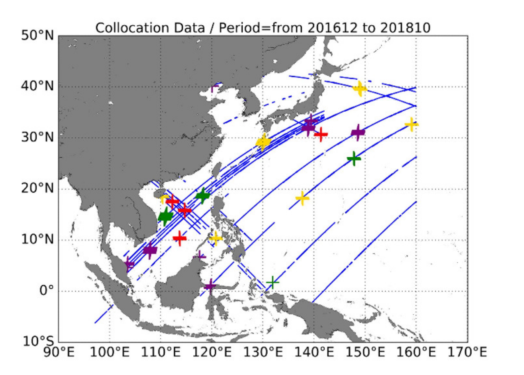Figure 1 shows the location map of the InIRA data and the collocated data of the four traditional altimeters. As indicated in the figure, the datasets are mainly concentrated in the coastal areas of Southeast Asia. A brief introduction of the various data mentioned above is given below.

2.1. InIRA

The InIRA is a Ku-band spaceborne side-looking radar with incidence angles ranging from 2° to 8°. It configures two antenna beams used for interferometric processing, which facilitate SSH measurement. It is also a synthetic aperture radar, affording high azimuth resolutions. Using interferometric and synthetic aperture technology, the InIRA can measure ocean SSH with a high spatial resolution in both the range and azimuth directions (30 m × 30 m). The InIRA data used in this study were intermittently collected from December 2016 to October 2018 in different tracks. In preparation for the analysis and retrieval, each InIRA dataset was divided into images with a dimension of approximately 5 km. Then, the parameters used were extracted from each image, and collocated data were obtained through linear interpolation according to the center of the image.

2.2. WW3

WW3 data are frequently used global-gridded model data. They can provide rich collocated data for remote sensing observations at any time and location in the ocean. Although model data have more uncertainty than the in situ data, they can still describe the data trends through the statistical characteristics of big data. Thus, these collocations from a model are useful in developing empirical models, particularly when there are few in situ observations. In this study, we followed this concept of using WW3 data for providing collocated waves in developing the model. Here, the used wave parameters include SWH and wave direction at 0.5° and 1 h. They were matched to the InIRA image center via spatial and temporal interpolations.

2.3. Traditional Altimeters

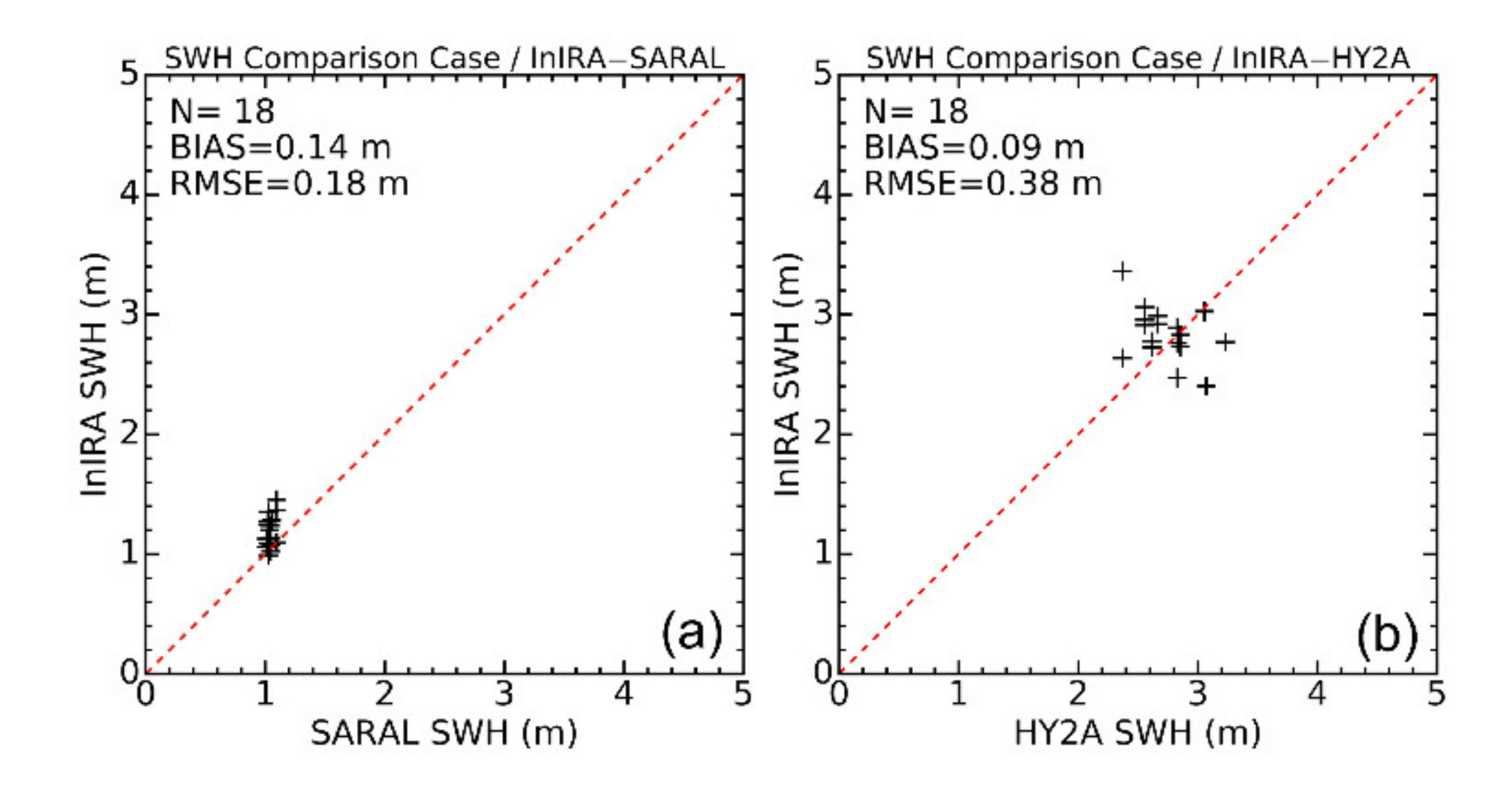
Traditional altimeters have been widely used for accurate SWH measurements based on the waveform of radar returns. Owing to their high accuracy, SWH data from traditional altimeters are commonly used for validating retrievals from SARs. In this study, these traditional altimeter SWH measurements were also used to validate InIRA SWH retrievals. Data from four types of traditional altimeters (JASON2, JASON3, SARAL, and HY2A) were used and collocated with the InIRA image center using the criteria of 3 h and 20 km. For the SARAL altimeter, Ka-band SWH data were used, while Ku-band SWH data were used for the rest. These traditional altimeter SWH data were downloaded with Geophysical Data Record (GDR) standard products. We directly used these data without any correction, assuming that these products have good quality.

2.4. ETOPO1 Data

ETOPO1 is a global elevation model that provides elevation data including land topography and ocean bathymetry with a spatial resolution of 1 arc. In this study, ETOPO1 data were used to distinguish between land and ocean. The ocean depth was extracted by interpolating the model data according to the InIRA image center. In preparing for collocations, only the data with water depths of less than −50 m were used.

3. Modeling

Based on previous studies on SARs [12,13,14,15], the ocean SWH can be estimated by establishing an empirical relationship to the SAR observed parameters. Motivated by these methods, this study employed an empirical model to estimate the SWH. The modulation functions for the InIRA data were first analyzed to determine the model input parameters.

From the radar ocean wave modulation theory, the InIRA data were modulated by four wave effects including tilt, hydrodynamic, range bunching, and velocity bunching modulations [35,36,37,38]. These four modulations, respectively, arise from the local incidence angle change induced by the long wave slope, hydrodynamic interaction between short and long waves, effective backscattering area change due to the long wave slope, and displacement of the backscattering facet by the long wave orbital velocity. The first two are due to the cross-section change, while the last two are from the area change and orbit motion of water particles, respectively. The first two modulation functions applied for the InIRA are different from those of the conventional SAR at moderate incidence angles and need to be deduced by the quasi-specular scattering theory at low incidence angles. For the last two, the InIRA modulation function are the same as that for the SAR, as they are independent of the sea surface scattering mechanism.

The tilt, range bunching and velocity bunching modulation functions for the InIRA data were derived. The first is deduced from a quasi-specular scattering mechanism in studies on OWSs [4,5,6,7]. For the last two, they are the same as that applied on the SAR. However, the hydrodynamic modulation function suitable for low incident InIRA data has not been proposed. The hydrodynamic modulation function at moderate incidence angles is proposed based on the Bragg scattering mechanism in the framework of a complex weak interaction theory [36]. Following this concept, the hydrodynamic modulation at low incidence angles should consider quasi-specular scattering in similar frameworks. In this case, the deduction for hydrodynamic modulation is very complex. On the other hand, the hydrodynamic modulation is usually considered relatively weak in long wave retrieval studies based on quasi-specular mechanism. This modulation is thus neglected and seen as an error source of wave retrievals. For examples, in long-wave retrieval for CFOSAT SWIM (with incidence angles from 0° to 10°) [7] and Sentinel-2 Multi-Spectral Instrument (sun glitter imagery) [39], both of them only consider the tilt modulation. From the above analysis, we realized that the hydrodynamic modulation for InIRA is probably weak and complex. To reduce the analysis difficulty, we neglected the hydrodynamic modulation and only used the tilt, range bunching and velocity bunching modulations to explore the SWH empirical model. The possible implications for SWH retrieval due to the neglect were arranged in Discussion. The following describes the specific analysis of the three modulation functions.

From previous studies, the InIRA tilt modulation function $T^{tilt}$ can be expressed as [4,5,6,7]

$$T^{tilt}\left(k\right)=\mathsf{\alpha }\left(\theta \right)k_x$$

(1)

where:

$$\alpha \left(\theta \right)=\cot \theta -4tan\theta -\frac{1}{co{s}^2\theta }\frac{\partial lnP\left(tan\theta ,0\right)}{\partial tan\theta }$$

(2)

The range bunching modulation function $T^{rb}$ can be expressed as [37]

$$T^{rb}\left(k\right)=\frac{\mathrm{i}{k}_x}{tan\theta }$$

(3)

Here, $k_x$ is the range component of wave number k, $\alpha$ is a scaling factor, $\theta$ is the incidence angle, and P is the probability density function of wave slopes.

Meanwhile, the InIRA velocity bunching modulation function $T^{vb}$ can be expressed as [9]

$$T^{vb}\left(k\right)=-\beta k_y\omega \left(cos\theta -i sin\theta \frac{k_x}{k}\right)$$

(4)

where:

$$w^2=gk$$

(5)

$$\beta =\frac{R}{V}$$

(6)

where $k_y$ is the azimuth component of k, g is the acceleration of gravity, R is the slant range, and V is the satellite velocity. For the InIRA, $\theta <8^{\mathrm{o}}$; therefore, $sin\theta \frac{k_x}{k}\ll cos\theta$. In this case, Equation (4) can be approximated as

$$T^{vb}\left(k\right)=-\beta k_y\sqrt{gk}cos\theta$$

(7)

Equations (1) and (3) show that the tilt and range bunching modulations are only related to the range component of waves, while Equation (7) shows that the velocity bunching modulation is only related to the azimuth component. When there are only waves toward the range direction, the transfer relation between the InIRA image spectra $P\left(k\right)$ and wave spectra $F\left(k\right)$ can be described in terms of tilt and range bunching modulation by

$$P\left(k\right)={\mathrm{e}}^{-k_y^2{\xi }^{,2}}({\mathsf{\alpha }}^2\left(\theta \right)+\frac{1}{ta{n}^2\theta })k_x^{2}F\left(k\right)$$

(8)

Similarly, when there are only waves toward the azimuth direction, the transfer relation can be described in terms of velocity bunching modulation by

$$P\left(k\right)={\mathrm{e}}^{-k_y^2{\xi }^{,2}}{\beta }^2{k}_y^{2}gkco{s}^2\theta F\left(k\right)$$

(9)

From above analysis, InIRA has a weak cutoff effect owing to the low satellite altitude, however, we still added the cutoff factor (${\mathrm{e}}^{-k_y^2{\xi }^{,2}}$) for improving retrieval accuracy according to quasi-specular SAR ocean mapping relation [9,10,11]. The ${\xi }^{,2}$ is the mean square azimuthal displacement of a scattering element, which can be estimated using cutoff ${\lambda }_c$ by [40]

$${\xi }^{,2}={\left(\frac{{\lambda }_c}{\pi }\right)}^2$$

(10)

Here, the ${\lambda }_c$ can be estimated by fitting the azimuthal autocorrelation function using a Gaussian function (Equation (7) of [40]). As we know, the SWH can be estimated by integrating F(k) as

$$SWH=4\sqrt{\iint F\left(k\right)d{k}_x\mathrm{d}{k}_y}$$

(11)

Using Equations (8), (9) and (11), the measured SWH for waves toward the range direction ($SW{H}_{tilt+rb}$) and azimuth direction ($SW{H}_{vb}$) can be estimated, respectively, by

$$SW{H}_{tilt+rb}=\frac{4tan\theta }{\sqrt{{\alpha }^2\left(\theta \right)ta{n}^2\theta +1}}\sqrt{\iint \frac{{\mathrm{e}}^{k_y^2{\xi }^{,2}}P\left(k\right)}{k_x^2}d{k}_x\mathrm{d}{k}_y}$$

(12)

$$SW{H}_{vb}=\frac{4}{\sqrt{{\beta }^{2}gco{s}^2\theta }}\sqrt{\iint \frac{{\mathrm{e}}^{k_y^2{\xi }^{,2}}P\left(\mathrm{k}\right)}{k_y^{2}k}d{k}_x\mathrm{d}{k}_y}$$

(13)

We defined two image spectra-related integration factors. The first is the range integration factor ($I{F}_{range}$) and the second is the azimuth integration factor ($I{F}_{azimuth}$):

$$I{F}_{range}=\sqrt{\iint \frac{{\mathrm{e}}^{k_y^2{\xi }^{,2}}P\left(\mathrm{k}\right)}{k_x^2}d{k}_x\mathrm{d}{k}_y}$$

(14)

$$I{F}_{azimuth}=\sqrt{\iint \frac{{\mathrm{e}}^{k_y^2{\xi }^{,2}}P\left(\mathrm{k}\right)}{k_y^{2}k}d{k}_x\mathrm{d}{k}_y}$$

(15)

Substituting Equations (14) and (15) into Equations (12) and (13), the two SWH expressions can be rewritten as

$$SW{H}_{tilt+rb}=\frac{4tan\theta }{\sqrt{{\alpha }^2\left(\theta \right)ta{n}^2\theta +1}}I{F}_{range}$$

(16)

$$SW{H}_{vb}=\frac{4}{\sqrt{{\beta }^{2}gco{s}^2\theta }}I{F}_{azimuth}$$

(17)

From the above two Equations, the SWH can be represented as a one-order function of $I{F}_{range}$ (for waves toward the range direction) or $I{F}_{azimuth}$ (for waves toward the azimuth direction) when the incidence angle is constant. In the actual modeling process, we do not expect a perfect first-order relationship between them. As long as there is a linear dependence between them, which can be used for modeling by fitting. Below, we attempt to confirm the linearity of the dependence by analyzing the InIRA data.

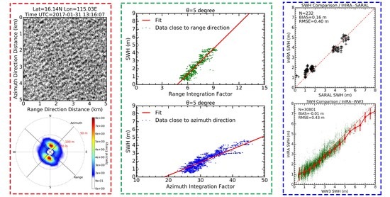
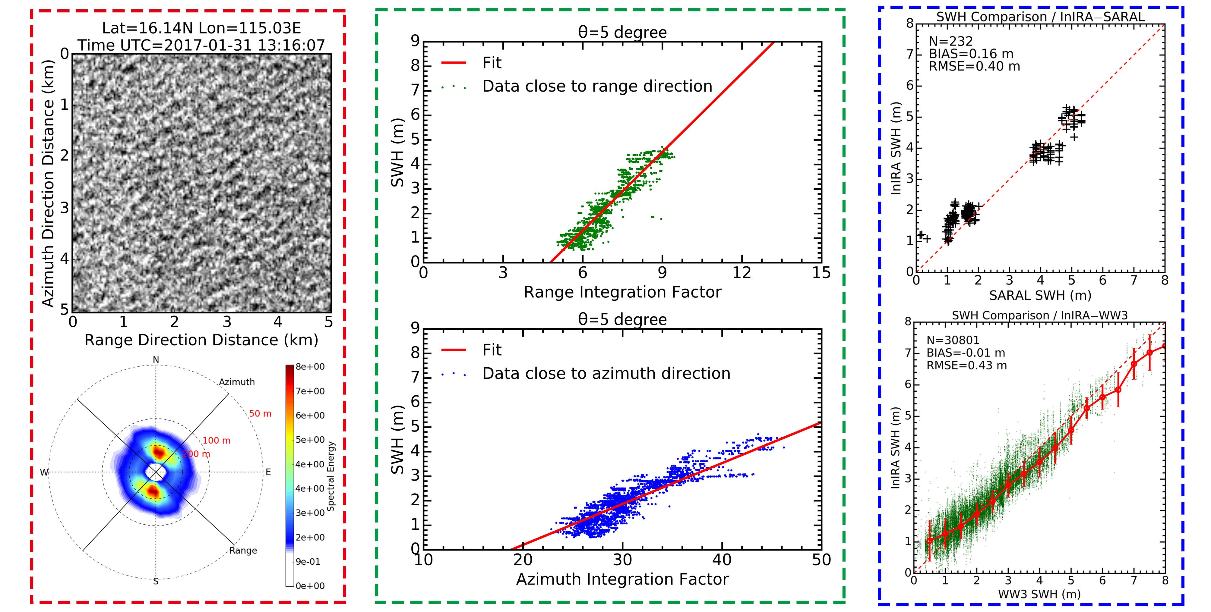
Figure 2 depicts two cases of InIRA data in terms of NRCS image and image spectra. Based on the spectra distribution, we believe that the first case (Figure 2a,b) is for a swell from the concentrated energy distribution, and the second case (Figure 2c,d) is for crossing wind waves from the dispersed energy distribution. Here, the swell case shows clearer wave-like stripes than the crossing wind wave case due to the mixing of the two wave systems. Both cases exhibit clear image spectra patterns. This indicates that the InIRA can image ocean waves similar to the SAR.

From the image spectra presented in Figure 2b,d, there is a weak cutoff phenomenon in the azimuth similar to that of the SAR, but the spectra patterns are still relatively complete (the spectra edges are not cutoff abruptly). In the SAR ocean wave imaging theory, the cutoff is attributed to the azimuthal displacement of the apparent position of a backscattering element. It determines the minimum detectable wavelength for the InIRA or SAR data. The cutoff wavelength in Figure 2c is only approximately 80 m, whereas the conventional SAR cutoff is approximately 150–200 m in the azimuth direction [7]. This shows that the InIRA cutoff is weaker than that of the SAR. As the InIRA has a lower satellite altitude (between 380 and 400 km) than the conventional SAR (with an altitude of approximately 755 km for the Gaofen-3 SAR), which brings a small cutoff factor as described in Equation (56) of [9]. To a certain extent, it helps to reduce the cutoff effects in Equations (8) and (9).

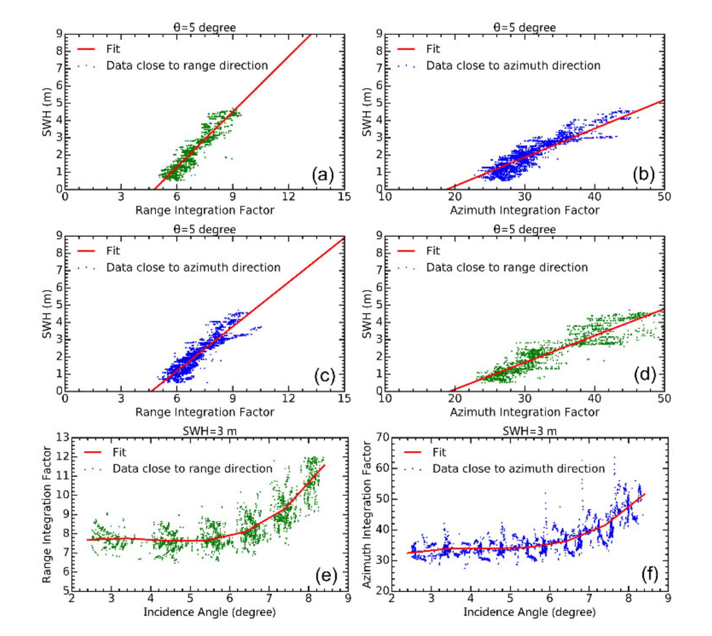
Based on the estimated image spectra, the two integration factors ($I{F}_{range}$ and $I{F}_{azimuth}$) were calculated using Equations (14) and (15). Note that only the image spectra with wavelengths from 30 m to 500 m were preserved in the calculation, while the rest were removed as interference information. Then, some dependence analyses were performed for confirming the relation between SWH and the two integration factors. First, Figure 3a,b illustrate the dependence of SWH on $I{F}_{range}$ and $I{F}_{azimuth}$, respectively. To ensure that the analysis of $I{F}_{range}$ was performed in the cases dominated by tilt and range bunching modulation, only the data close to the range direction (with relative wave directions between 0° and 15°) were used. Similarly, the analysis of $I{F}_{azimuth}$ was performed using data close to the azimuth direction (with relative wave directions between 75° and 90°), making the velocity bunching the dominant modulation. The relative wave direction was defined as the angle between the wave direction (from WW3 data) and range direction (from InIRA auxiliary data). By using 180° symmetry feature of radar returns, the relative wave direction was converted and concentrated into the range of 0°–90°. The concentration of data helps plotting clear trends, especially when the data are limited. From the two figures, the SWH increases with both $I{F}_{range}$ and $I{F}_{azimuth}$ with an approximate one-order function. This is basically consistent with the theoretical dependence in Equations (16) and (17). Comparing the two, the dependence on $I{F}_{range}$ is clearer. These dependences reveal the potential of using the $I{F}_{range}$ or $I{F}_{azimuth}$ factor to build an SWH model.

We further conducted a similar analysis for Figure 3c,d; however, the data used were exchanged with each other. In this case, Figure 3c shows a bifurcated trend, whereas the trend in Figure 3d is more dispersed than that in Figure 3b. Although there are still some dependences, they are significantly weaker than those in Figure 3a,b. This means that the $I{F}_{range}$ factor is more suitable for describing waves in the range direction, whereas the $I{F}_{vb}$ factor is more appropriate for those in the azimuth direction. This also indicates that the single factor defined in this study cannot describe waves in different directions simultaneously. The two factors should be considered together for estimating the SWH.

Figure 3e,f depict two integration factor dependences on the incidence angles, in which the SWH is at 3 m. From Figure 3e, the $I{F}_{range}$ is basically constant at first and then increases with incidence angles larger than 6°. From Figure 3f, the $I{F}_{azimuth}$ shows a similar trend with $I{F}_{range}$. This means that the relationship between the SWH and each integration factor varies with the incidence angle. The incidence angle should also be considered in building the SWH model.

From the above analysis, the SWH increases with both $I{F}_{range}$ and $I{F}_{azimuth}$, and the relationships between them vary with the incidence angle. In particular, the SWH values in the range and azimuth directions are more dependent on $I{F}_{range}$ and $I{F}_{azimuth}$, respectively. In the framework of the linear ocean wave theory, any wave can be divided into two components in the range and azimuth directions. We considered combining the $I{F}_{range}$ (describing the wave component in the range direction) and $I{F}_{azimuth}$ (describing the wave component in the azimuth direction) factors to build an empirical SWH model. We inferred that there is a coupling effect between the range modulation (tilt and range bunching) and azimuth modulation (velocity bunching) based on previous SAR studies on the wave transfer relation. Thus, we used a quadratic orthogonal polynomial to model the coupling effect. To reduce the modeling difficulty, the model was segmented using the incidence angle at steps of 0.5°. The final model function was described by

$$SWH\left(\theta \right)={\displaystyle \sum }_{i=0}^2{\displaystyle \sum }_{j=0}^2{C}_{ij}\left(\theta \right)I{F}_{range}^i\left(\theta \right)I{F}_{azimuth}^j\left(\theta \right)$$

(18)

where $C_{ij}$ are model coefficients.

The model coefficients in Equation (18) were estimated by fitting randomly selected 50% collocations consisting of InIRA and WW3 data. Note that the InIRA data collocated with traditional altimeter data were not used for fitting, as they were reserved for an independent validation later. The estimated model coefficients are listed in

Table 1. Model coefficients.

θ	Coefficients
	C00	C01	C02	C10	C11
3.0	18.7429	1.2219	−0.0674	−14.1237	0.3946
3.5	−7.8974	0.3638	−0.0079	0.2710	0.0425
4.0	−5.2364	0.7547	−0.0202	−2.5837	0.0543
4.5	−8.6532	0.8836	−0.0347	−2.2180	0.1302
5.0	−6.0010	0.1629	−0.0060	0.7164	0.0451
5.5	−10.9052	−0.1861	−0.0079	3.8535	0.1082
6.0	−6.2796	−0.2861	−0.0066	3.0292	0.1116
6.5	−6.2745	0.0239	−0.0008	1.4898	0.0112
7.0	−6.6263	0.1313	0.0015	1.0007	−0.0250
θ	Coefficients
	C12	C20	C21	C22
3.0	0.0049	0.9756	−0.0394	0.0001
3.5	0.0001	−0.1023	−0.0001	−0.0000
4.0	0.0017	0.2547	−0.0092	−0.0000
4.5	0.0029	0.1498	−0.0148	−0.0000
5.0	0.0000	−0.1234	−0.0002	−0.0000
5.5	−0.0001	−0.5080	0.0008	−0.0000
6.0	−0.0002	−0.4525	0.0009	−0.0000
6.5	−0.0000	−0.1025	0.0003	−0.0000
7.0	0.0000	0.0138	0.0002	−0.0000

.

4. Results

4.1. Retrieval

The remaining 50% of the collocations were used to validate the retrievals. The SWHs were retrieved from the InIRA data using the proposed model. They were compared with the collocated WW3 and traditional altimeter data. The retrieval process is simple. The extracted two integration factors and incidence angle were substituted into the model in Equation (18), through which the SWH could be easily obtained. Note that the model coefficients were obtained through linear interpolation according the incidence angles.

4.2. Validation

For the validation, a case study and an overall comparison were performed separately. Figure 4 presents the case study using the collocated traditional altimeter data. In this case, SARAL and HY2A altimeter data were collocated with the InIRA data, according to the criteria mentioned above. The beginning time for the InIRA data acquisition is 31 January 2017 at 13:16:33 UTC. The collocated positions with HY2A data are located in deep-sea areas, while the positions with SARAL are in offshore areas. As the SWH values for these collocations are overlapping, we plotted every type of SWH data on a separate figure for a clearer comparison. Meanwhile, its collocated data track was plotted with a black line, to clearly determine the intersection position. As shown in Figure 4, the SWH data from the InIRA have good agreement with the two traditional altimeter collocations. The statistical errors were calculated (Figure 5). The RMSEs of the InIRA SWH compared with the SARAL and HY2A data are 0.18 m and 0.38 m, respectively, indicating that the SWH retrieval accuracy with the application of the proposed model is acceptable.

Furthermore, the statistical errors for all collocations were calculated. The InIRA SWH errors with WW3 data are first shown (Figure 6). The WW3 model data provide rich collocations and helped in analyzing the overall accuracy. The figure reveals consistency between the InIRA retrievals and WW3 data, with an RMSE of 0.43 m and a slight bias of −0.01 m. The differences mainly occur at two ends (smaller than 1.0 m and larger than 3.5 m). For the lower SWH range, the InIRA SWH is on the high side, whereas it is on the low side for the higher SWH range. We think that this is possibly due to the varying SWH dependence in different SWH ranges. Overall, the InIRA SWH retrievals are consistent with the WW3 data.

The comparison with WW3 data was reanalyzed for determining the retrieval accuracy trends with different incidence angles and relative wave directions (Figure 7). Here, the incidence angle range is from 2.5° to 7.5°, while some data at the edge of the beam were removed for ensuring data quality. Additionally, the relative wave direction range is from 0° to 90°, for which the 0° and 90° represents the range direction and azimuth direction, respectively. It has the same definition as one in Figure 3. From Figure 7a,b, we found that both BIAS and RMSE vary with incidence angles. In particular, when the incidence angles were larger than 6.5°, the accuracies were significantly degraded (but still acceptable). From RMSE trends, the central beam (about 5.0°) has better accuracy than beams at both ends. It is probably due to the higher signal-to-noise ratio (SNR) of the central beam. From Figure 7c,d, we found that both BIAS and RMSE slightly oscillate with relative wave directions by an amplitude about 0.1 m. The accuracies at different relative wave directions are all acceptable. The BIAS at range and azimuth directions (0° and 90°) are better than ones at other directions, which are probably due to the model integration factors are more sensitive to wave components at the two directions. In addition, the RMSE in the azimuth direction (90°) is significantly higher than ones in other directions, which may be due to the residual cutoff effects from velocity bunching modulation.

In addition to the comparison with WW3 data, the InIRA SWH values were statistically compared with collocated traditional altimeter data, as illustrated in Figure 8. The figure shows that the statistical RMSEs with JASON2, JASON3, SARAL, and HY2A are 0.46, 0.55, 0.40, and 0.49 m, respectively. All BIASs are within 0.2 m. To obtain unified statistics, we simply averaged the RMSEs and BIASs of the data from the four types of traditional altimeters. The average RMSE and BIAS are 0.48 m and 0.02 m, respectively. The comparisons indicate that the retrieved InIRA SWHs also have consistency with the traditional altimeter data.

5. Discussion

In addition to the wide-swath SSH measurement, the InIRA has the potential for wave measurement because it can provide NRCSs with high spatial resolutions similar to the conventional SAR. The measured waves are useful in correcting the sea state bias of InIRA-derived SSHs and supplementing wave products from other spaceborne sensors. Currently, only a few studies involved the wave or SWH retrieval from InIRA data; thus, this study focuses on this aspect. From previous studies on SARs [8,9,10,11,12,13,14,15], there are generally two SWH retrieval approaches, namely the theoretical transfer relation and empirical model. In terms of SWH retrieval accuracy, the latter is better than the former, possibly because the latter handles the nonlinear and cutoff effects more effectively. Therefore, this paper proposed an empirical model to retrieve SWH data. Using the model, SWHs were retrieved from InIRA data and validated using both WW3 and traditional altimeter data. Through the validation, the InIRA SWH retrievals were found to have agreement with the collocated data, suggesting the potential of InIRA data for SWH retrieval.

In the comparisons between the InIRA SWH retrievals with traditional altimeter data, the average RMSEs of the InIRA SWH retrievals are within 0.5 m, which are comparable to SAR values using the empirical model approach. For instance, using the ERS2 SAR data, Schulz-Stellenfleth et al. [12] proposed an empirical model (CWAVE2.0) to estimate the SWH, which results in an RMSE of approximately 0.5 m compared to WAM model data. Following this approach, Li et al. [13] use the CWAVE_ENV model to obtain an RMSE of approximately 0.5 m for ENVISAT SAR data compared to traditional altimeter data. Stopa and Mouche [14] used the CWAVE_S1A model and obtain RMSEs within 0.5 m for Sentinel-1A SAR data compared to traditional altimeter and buoy data. These comparisons suggest that both the InIRA and SAR can provide acceptable SWH retrieval accuracies using the empirical model, although they follow different backscattering mechanisms (quasi-specular and Bragg).

This study found the dependences between the SWH and two factors, range and azimuth integration, which were further confirmed from the InIRA data. On this basis, an orthogonal empirical model using the two integration factors as inputs was proposed. This model adopted a concept of orthogonal decomposition, which has not been widely applied in empirical models [12,13,14,15]. In our attempt, the model obtained an acceptable retrieval accuracy, which indicates that SWH can be modeled by combining the two orthogonal integration factors calculated from image spectra. This concept concerning the orthogonal integration factors may be used for supplementing existing SAR and OWS SWH retrieval methods.

The InIRA NRCS image in this study exhibits clear wave-like stripes and complete image spectra, which indicates that the cutoff effect on the InIRA is significantly weaker than that on the conventional SAR. This is because the InIRA has a lower satellite altitude, which can be well explained by the known SAR ocean wave imaging theory. The small cutoff of the InIRA data confirmed this theory again. Nevertheless, owing to the limited coverage, the low-altitude SAR has not been widely used for ocean remote sensing observations. Currently, with the improvement in satellite technology and reduction in launch cost, a low-altitude satellite constellation that can effectively extend the data coverage through a combination of multiple satellites has become possible. In this case, the low-altitude constellation can simultaneously satisfy the requirements of weak cutoff effects and wide coverage, which may provide a new manner for measuring ocean wave fields.

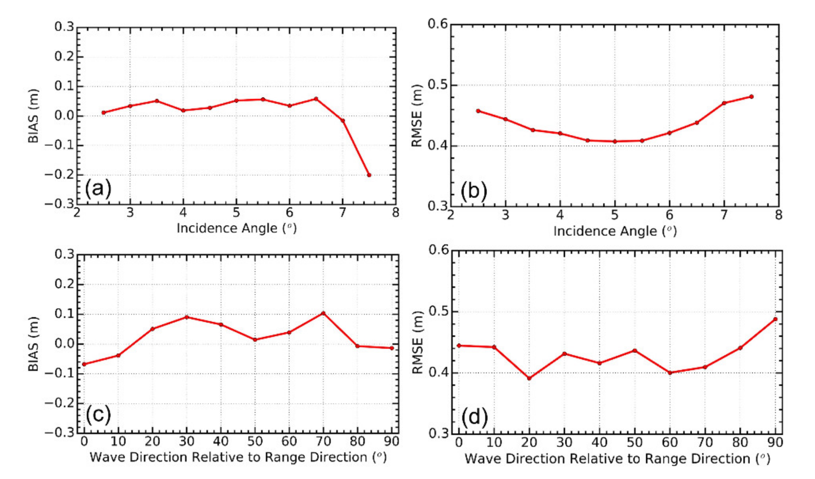
Despite the above findings, this study has three limitations. First, the hydrodynamic modulation was not considered owing to its complexity and weakness. Although our study adopted an empirical model, however, the model construct was based on the derivation from radar ocean wave modulation theory. Therefore, we think neglecting hydrodynamic modulation probably brings some errors. Based on previous studies [39], the hydrodynamic modulation first decreases, and then increases with incidence angles. It has the weakest value near 10°. It seems to mean that the error due to the neglect of hydrodynamic modulation, should decrease monotonously with incidence angles from 2.5° to 7.5°. However, Figure 7a,b show that the retrieval accuracy trends with incidence angles were not significantly monotonous. Therefore, we think that the retrieval error due to the neglect of hydrodynamic modulation are probably not the dominated one.

Second, the proposed model can extract SWH data, but not wave spectra. As is known, the wave spectrum contains complete wave information, which can be used to estimate any wave parameter [9]. It has wider applications than the single SWH parameter. From the preliminary analysis results presented in Figure 2, the InIRA can image the ocean surface and capture wave signatures. The cutoff effect is weak owing to the low altitude, and thus, the image spectra are relatively complete. We believe that the InIRA still has the possibility of retrieving wave spectra using the transfer relation. To achieve this, the main challenge is that of estimating the nonlinear effects and the hydrodynamic modulation function in the transfer relation. This issue can refer to related theoretical studies on SARs in [9]. It is noted that the quasi-specular scattering should be considered instead of the original Bragg scattering.

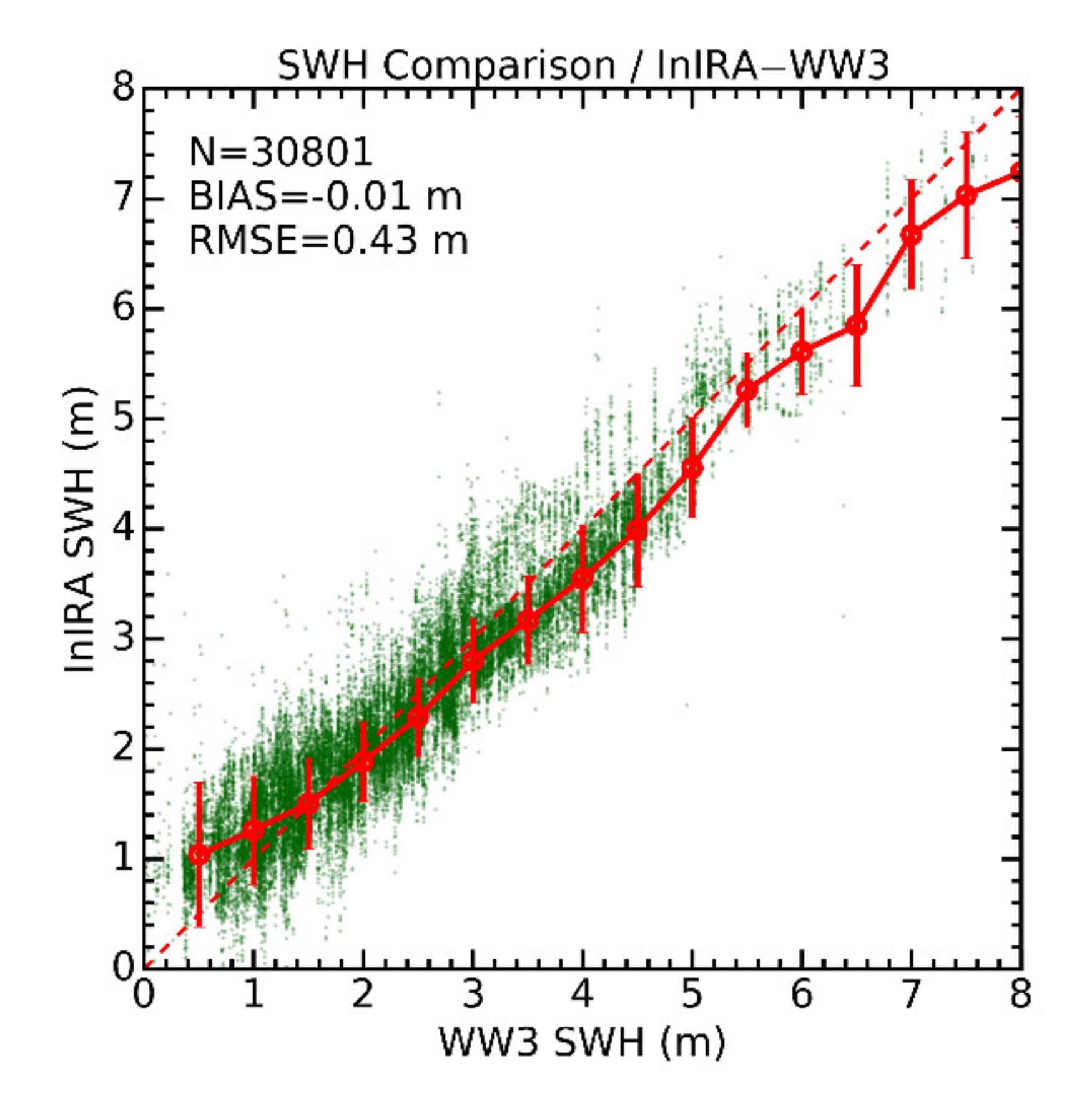
Third, some biases still exist between the retrievals and collocations, particularly for higher SWH ranges. From the comparison of the SWH retrieval presented in Figure 6, WW3 SWH data used for modeling are basically within 5.0 m. The proposed model will mainly be applicable for this range. Moreover, the high sea state is often accompanied by nonlinear effects, which may be caused by wave breaking. This nonlinearity effect on backscatter is very evident. For instance, the saturation of backscatter from SARs and scatterometers due to nonlinearity has been recognized [41]. This prompts researchers to explore other sensors for observing high winds. The sensors used include radiometers and SARs with cross-polarizations [42,43]. Low incident backscatter in the high sea state is also analyzed, and no clear correlation between backscatter and wind due to nonlinear effects is found [44]. From the above analysis, the bias in the high SWH range in this study is probably induced by the particularity of the SWH dependence in high sea states. When there are abundant data in high SWH ranges, the SWH dependence in the proposed model will be refined and the bias may be further improved.

6. Conclusions

This paper proposed an empirical model to retrieve SWHs from the InIRA aboard the Chinese Tiangong-2 space laboratory. The data used include the InIRA and collocated WW3 and traditional altimeters (JASON2, JASON3, SARAL, and HY2A).

First, the tilt, range bunching and velocity bunching modulations at low incidence angles were analyzed. From the analysis, the clear dependences between the SWH and two factors, range and azimuth integration, were found for waves in the range and azimuth directions, respectively. This type of dependence was further confirmed by the InIRA data. Finally, an orthogonal model using the two integration factors as model inputs was proposed. The model was segmented by the incidence angle and the model coefficients were estimated by fitting the collocations.

SWHs were retrieved from the InIRA data using the proposed model. These retrievals were validated using the collocated WW3 and traditional altimeter SWHs. Through the validation, the InIRA SWH was found to have an RMSE of 0.43 m compared with the WW3 SWH, and an average RMSE of 0.48 m compared with all traditional altimeter data. These comparisons revealed the potential of InIRA for measuring the SWH.

The main objective of the InIRA in oceanic applications is to measure the wide-swath SSH. In future work, the SWH retrievals from the proposed method will be used to correct the sea state bias of InIRA-derived SSH measurements.