
IMG2nDSM: Height Estimation from Single Airborne RGB Images with Deep Learning


1
CYENS Center of Excellence, Nicosia 1016, Cyprus
2
Department of Computer Science, University of Twente, 7522 NB Enschede, The Netherlands
3
Department of Computer Science, University of Cyprus, Aglantzia 2109, Cyprus
*
Author to whom correspondence should be addressed.
Remote Sens. 2021, 13(12), 2417; https://0-doi-org.brum.beds.ac.uk/10.3390/rs13122417
Submission received: 21 April 2021
/
Revised: 12 June 2021
/
Accepted: 17 June 2021
/
Published: 21 June 2021
Abstract
:Estimating the height of buildings and vegetation in single aerial images is a challenging problem. A task-focused Deep Learning (DL) model that combines architectural features from successful DL models (U-NET and Residual Networks) and learns the mapping from a single aerial imagery to a normalized Digital Surface Model (nDSM) was proposed. The model was trained on aerial images whose corresponding DSM and Digital Terrain Models (DTM) were available and was then used to infer the nDSM of images with no elevation information. The model was evaluated with a dataset covering a large area of Manchester, UK, as well as the 2018 IEEE GRSS Data Fusion Contest LiDAR dataset. The results suggest that the proposed DL architecture is suitable for the task and surpasses other state-of-the-art DL approaches by a large margin.
1. Introduction
Aerial images are widely used in geographic information systems (GIS) for a plethora of interesting tasks, such as: urban monitoring and planning [1,2,3], agricultural development [4], landscape change detection [5,6,7] and disaster mitigation planning and recovery [8], as well as aviation [9,10]. However, these images are predominantly two-dimensional (2D) and constitute a poor source of three-dimensional (3D) information, hindering the adequate understanding of vertical geometric shapes and relations within a scene. Ancillary 3D information improves the performance of many GIS tasks and facilitates the development of tasks that require a geometric analysis of the scene, such as digital twins for smart cities [11] and forest mapping [12]. In such cases, the most popular type of this complementary 3D information is the form of a Digital Surface Model (DSM). The DSM is often obtained with a Light Detection and Ranging Laser Scanner (LiDAR) or an Interferometric Synthetic-Aperture Radar (InSAR), a Structure-from-Motion (SfM) methodology [13], or by using stereo image pairs [14]. Structure from motion is a technique for estimating 3D structures from 2D image sequences. The main disadvantages of SfM include the possible deformation of the modeled topography, its over-smoothing effect, the necessity for optimal conditions during data acquisition and the requirement of a ground control point [15]. Like SfM, DSM estimation by stereo image pairs requires difficult and sophisticated acquisition techniques, precise image pairing and relies on triangulations from pairs of consecutive views. LiDAR sensors can provide accurate height estimations and have recently become affordable [16]. However, LiDAR sensors suffer from poor performance when complex reflective and refractive bodies (such as water) are present and can return irrational values in such cases, especially where there are multiple light paths from reflections in a complex scene. Despite these specific performance issues, LiDAR remains a commonly used technology for the acquisition of DSMs.
A substantial nontechnical disadvantage of obtaining aerial DSMs and DTMs of large areas with LiDAR technology is the high cost of the required flight mission. This cost factor can preclude LiDAR acquisition as economically prohibitive. Therefore, an elevation estimation from an input image is a compelling idea. However, a height estimation from a single image, as with monocular vision in general, is an ill-posed problem; there are infinite possible DSMs that may correspond to a single image. This means that multiple height configurations of a scene may have the same apparent airborne image [17] due to the dimensionality reduction in the mapping of an RGB image to a one-channel height map. Moreover, airborne images frequently pose scale ambiguities that make the inference of geometric relations nontrivial. Consequently, mapping 2D pixel intensities to real-world height values is a challenging task.
In contrast to the remote sensing research community, the computer vision (CV) community has shown a significant interest in depth estimation from a single image. Depth perception is known to improve computer vision tasks such as: semantic segmentation [18,19], human pose estimation [20] and image recognition [21,22,23], analogous to height estimations, improving remote sensing tasks. Prior to the successful application of Deep Learning (DL) for depth prediction, methods such as stereo vision pairing, SfM and various feature transfer strategies [24] have been used for the task. All these methods require expensive and precise data (pre)processing to deliver quality results. Contrastingly, DL simplifies the process while achieving a better performance. Eigen et al. [25] used a multiscale architecture to predict the depth map of a single image. The first component of the architecture was based on the AlexNet DL architecture [23] and produced a coarse depth estimation refined by an additional processing stage. Laina et al. [26] introduced residual blocks into their DL model and used the reverse Huber loss for optimizing the depth prediction. Alhashmin and Wonka [27] used transfer learning from a DenseNet model [28] pretrained on ImageNet [29], which they connected to a decoder using multiple skip connections. By applying multiple losses between the ground truth and the prediction, a state-of-the-art in-depth estimation from a single image was achieved. The interest of the CV community on depth estimation originated from the need for the better navigation for autonomous agents, space geometry perception and scene understanding, especially in the research fields of robotics and autonomous vehicles. Specifically, regarding monocular depth estimation, AdaBins [30] achieved state-of-the-art performances on the KITTI [31] and NYU-Depth v2 [32] datasets by using adaptive bins for depth estimation. Mahjourian et al. [33] used the metric loss feature for the self-supervised learning of depth and egomotion. Koutilya et al. [34] combined synthetic and real data for unsupervised geometry estimation through a generative adversarial network (GAN) [35] called SharinGAN, which maps both real and synthetic images to a shared domain. SharinGAN achieves state-of-the-art performances on the KITTI dataset.
The main approaches used by researchers in aerial image height estimations based on DL involve: (a) training with additional data, (b) tackling auxiliary tasks in parallel to the depth estimation, (c) using deeper models with skip connections between layers and (d) using generative models (such as GANs) with conditional settings.
Alidoost et al. [36] applied a knowledge-based 3D building reconstruction by incorporating additional structural information regarding the buildings in the image, like lines from structure outlines. Mou and Zhu [37] proposed an encoder–decoder convolutional architecture called IM2HEIGT that uses a single, but provenly functional, skip connection from the first residual block to the second-to-last block. They argue that both the use of residual blocks and a skip connection contributes significantly to the model performance. The advantages of using residual blocks and skip connections were also highlighted in the works of Amirkolaee and Arefi [38] and Liu et al. [17], who also used an encoder–decoder architecture for their IM2ELEVATION model. Liu et al. additionally applied data preprocessing and registration based on mutual information between the optical image and the DSM.
Furthermore, multitask training has proven to be beneficial, especially when the height estimation is combined with image segmentation. Srivastava et al. [39] proposed a joint height estimation and semantic labeling of monocular aerial images with convolutional neural networks (CNNs). Carvalho et al. [40] used multitask learning for both the height prediction and the semantics of aerial images. A different approach to the height estimation problem used a generative model that produced the height map of an aerial image when given the image as the input. This strategy employs the conditional setting of the GAN and performs image-to-image translation, i.e., the model translates an aerial image to a DSM. Ghamisi and Yokoya [41] used this exact approach for their IMG2DSM model. Similarly, Panagiotou et al. [42] estimated the Digital Elevation Models (DEMs) of aerial images.
2. Materials and Methods
This section discusses the datasets used to train and evaluate the model, the technical aspects of the methods and the techniques used in the Deep Learning model. The model’s architecture is also presented, along with the task-specific design features that make it appropriate for height predictions. For further information on neural networks and Deep Learning, please refer to references [43,44].
2.1. Datasets and Data Pre-Processing
Two relatively large datasets were used to develop and evaluate the proposed height prediction model, namely: a Manchester area dataset, compiled by the authors, and an IEEE GRSS data fusion contest dataset. The focus of the Manchester area dataset is on estimating the height of buildings, while the focus of the IEEE GRSS data fusion contest dataset is on estimating the height of all objects in the images.
2.1.1. Manchester Area Dataset
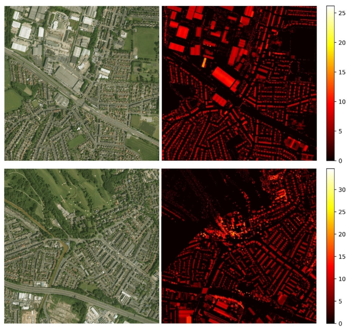
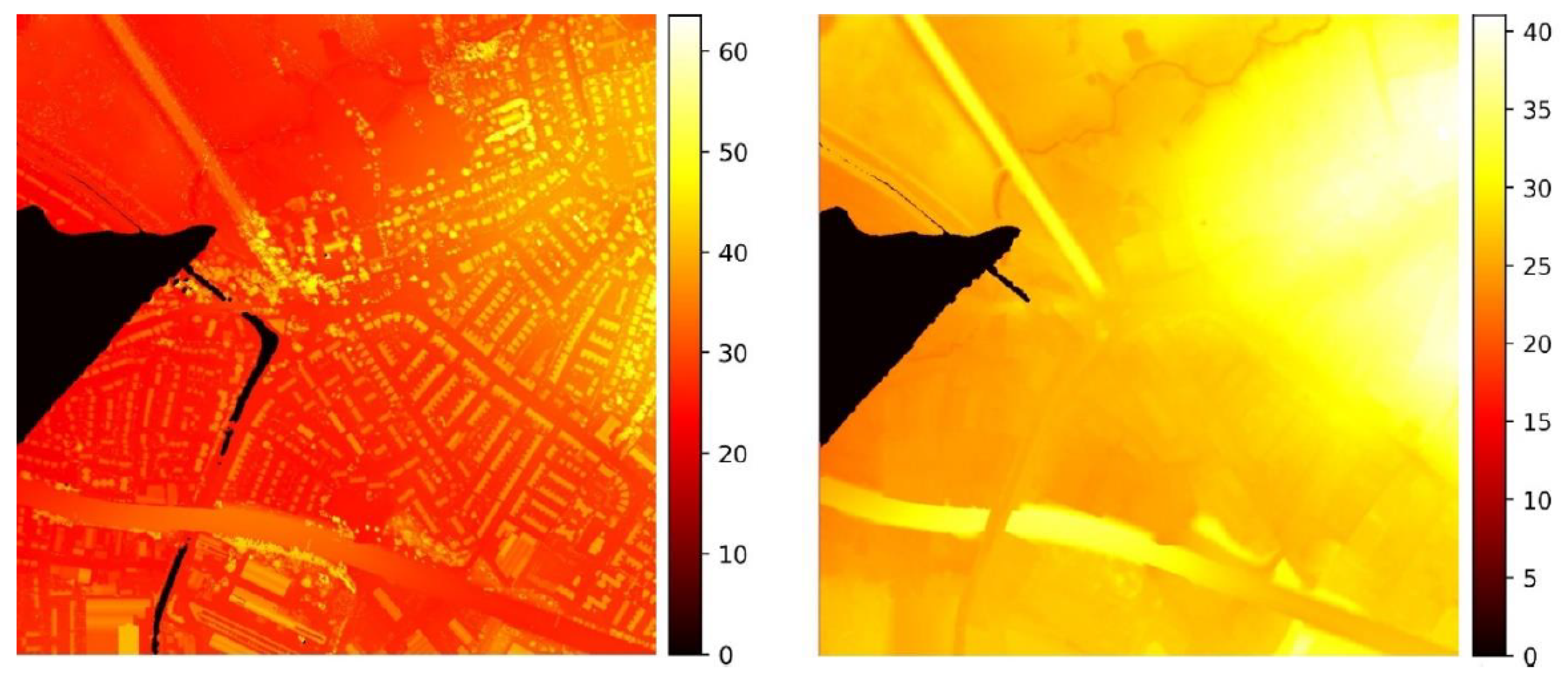
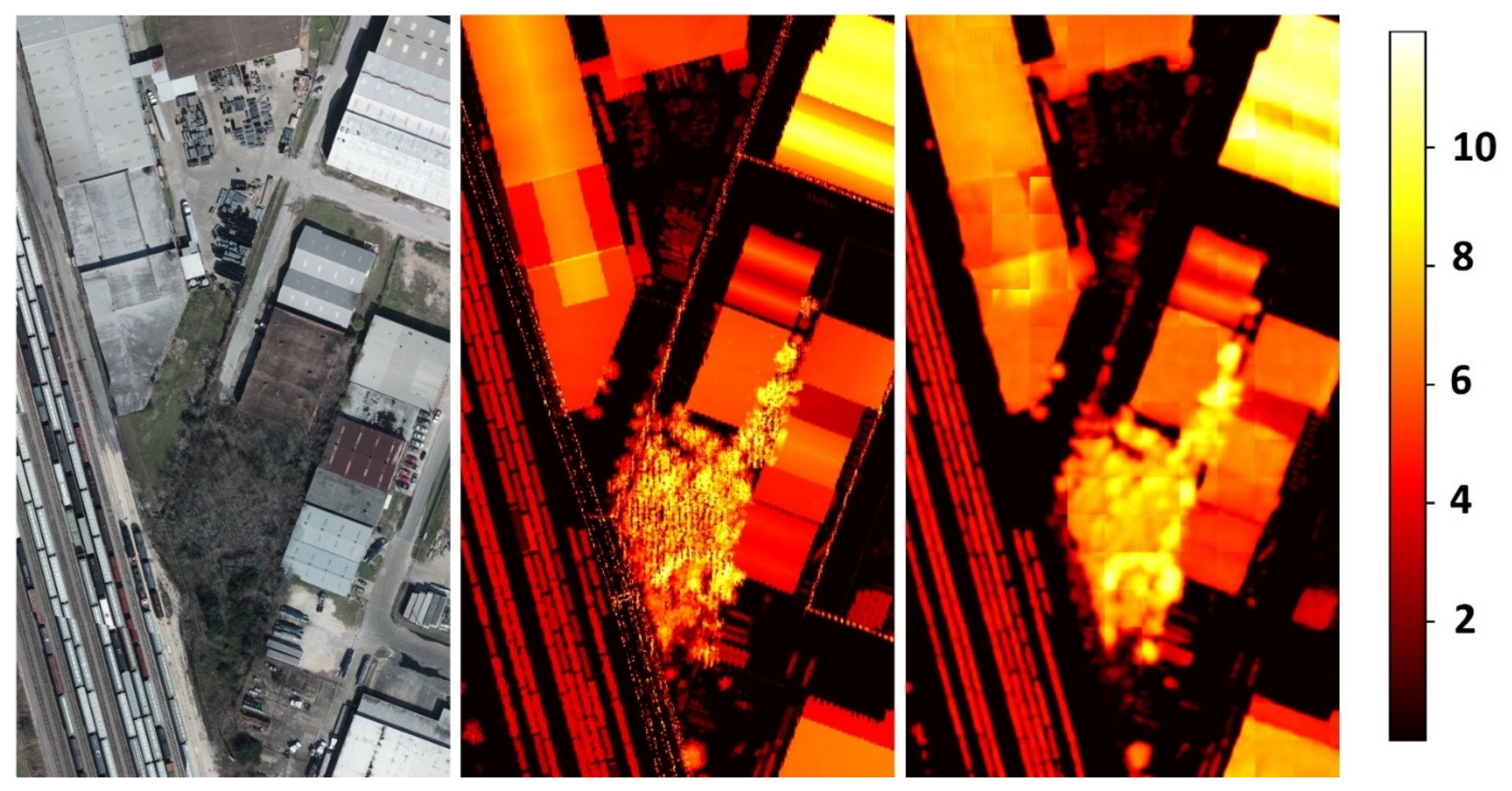
The first dataset used to train the model comprised images and LiDAR DEMs (DSMs and DTMs), all from the Trafford area of Manchester, UK. The aerial photography was from Digimap [45] (operated by EDINA [46]). Both the LiDAR DEMs and the RGB images were geospatially aligned according to the Ordnance Survey National Grid reference system, a system using a transverse Mercator projection with a straight-line grid system built over an Airy 1830 ellipsoid. The reference grid system choice was essentially arbitrary, as the model used input image sections small enough for alignment deviations to be insignificant. Furthermore, as the model was trained to build nDSMs from the input images, model nDSM outputs were aligned to the image pixel locations. The LiDAR data belongs to the UK Environment Agency [47]. It covered approximately 130 km2, comprising roughly 8000 buildings. The RGB images had a resolution of 0.25 m by 0.25 m, and the LiDAR resolution was 1 m by 1 m. The RGB images and the LiDAR maps were acquired at different dates; hence, there were data inconsistencies resulting from new constructions or demolished buildings. Such inconsistencies constituted a barrier to the training of a DL model, yet were representative of real-world problems, especially given that many wide-area LiDAR datasets are compiled as composite images from LiDAR flights on multiple dates. Due to the low LiDAR resolution, this dataset was not appropriate for estimating the height of vegetation; thus, the analysis focused only on buildings. Since segmentation labels for the differentiation of what was vegetation and what was not were not available, a threshold height value of 1.5 m was used to distinguish buildings. This approach occluded low vegetation and cars, which was desirable, since the cars were mobile objects and, thus, the source of additional inconsistency. Furthermore, vegetation was a highly variable entity that was easily removed from the environment and was not necessary for many applications. The model was trained with RGB aerial images as the input and the normalized DSMs (nDSM = DSM-DTM) as the target. nDSMs ignore the altitude information of the terrain and concentrate on the heights of objects. Figure 1 shows examples of different areas from the Manchester dataset and their corresponding ground truth nDSMs. Figure 2 shows the DTM and DSM of Figure 1 (bottom image) and demonstrates some flaws in their specific dataset.
2.1.2. IEEE GRSS Data Fusion Contest Dataset
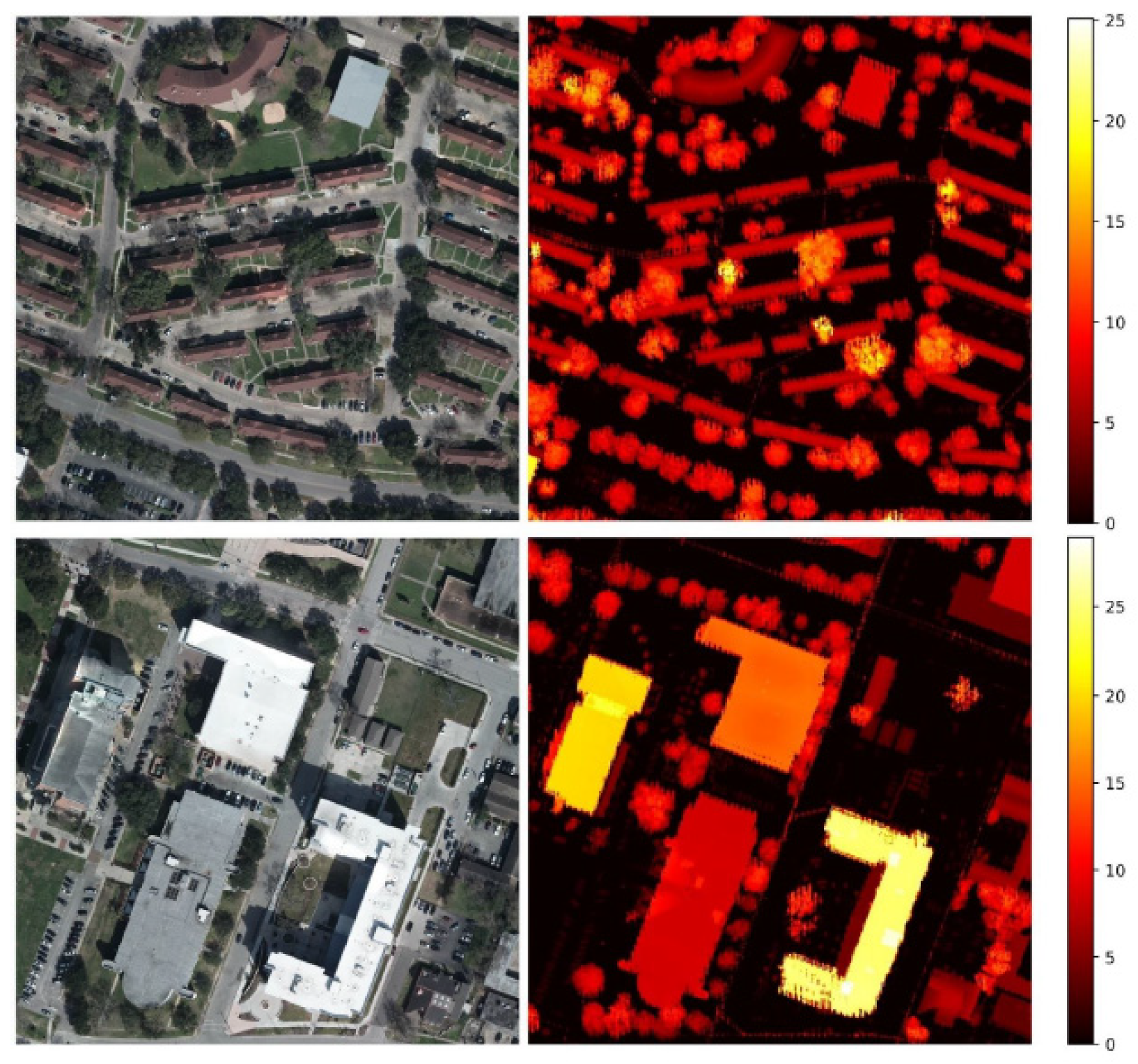
The Data Fusion 2018 Contest Dataset (DFC2018) [48,49] is part of a set of community data provided by the IEEE Geoscience and Remote Sensing Society (GRSS). The Multispectral LiDAR Classification Challenge data was used herein. The RGB images in the dataset had a 0.05 m by 0.05 m resolution, and the LiDAR resolution was 0.5 m by 0.5 m. The data belonged to a 4.172 × 1.20 (2 km2) area. Given the higher resolution of the RGB images, this dataset was more suitable for estimating the vegetation height than the Manchester area dataset. Figure 3 shows example pairs of RGB images and their corresponding nDSMs from this dataset. The ratio between the resolution of the RGB images and the resolution of their corresponding LiDAR scans affected the design of the depth-predicting model. Like in the Manchester area dataset, the model must handle the resolution difference between its input and its output and predict a nDSM that is several times smaller than the RGB image. Since the two datasets have different resolutions between the RGB images and the LiDAR scans, the same model cannot be used for both cases. Consequently, the models differ in their input/output sizes and the resolution reduction they must apply. For the most part, the models used for the two datasets are very similar, but slight architectural modifications are applied to cope with the resolution differences.
2.2. Data Preparation
The model operating on the Manchester area dataset used image patches of sizes 256 × 256 × 3, while the model operating on the DFC2018 dataset used image patches of sizes 520 × 520 × 3. The specific input sizes determined that the former model output a map of size 64 × 64 and the latter had an output of 52 × 52, since the resolution ratios of the images to LiDAR datasets were 4 and 10, respectively: every 4 pixels in one aerial image of the Manchester dataset correspond to 1 pixel in the respective nDSM, and 10 pixels in one aerial image of the DFC2018 dataset corresponded to 1 pixel in the respective nDSM. The 64 × 64 and the 52 × 52 sizes of the model outputs offered a compromise between the computational and memory requirements during training and sufficient scenery area consideration when calculating a nDSM, i.e., basing the estimation on several neighboring structures in the input image for achieving better accuracy. Various output sizes were experimented with, and it was discovered that predicting larger nDSMs tends to achieve a slightly better accuracy at the cost of increased memory usage and computational requirements.
2.3. Model Description
In this section, the technical aspects of the methods and techniques used in the proposed DL model are discussed. The model’s architecture is presented, together with the task-specific design features that make it appropriate for depth prediction. The authors call the model presented herein “IMG2nDSM”, because it maps an aerial photography image to a nDSM.
The proposed architecture shares some similarity with semantic segmentation models, where the model must predict the label of each pixel in an image and, thus, partition it into segments. The segmentation may have the size of the input image or a scaled-down size. In this study, instead of labels, the real values corresponding to the elevation of each pixel were predicted in a down-scaled version of each RGB image. As with the semantic segmentation task, several DL models are suitable for learning the task of predicting nDSM values. A popular DL architecture, the U-Net model [50], was chosen due to its efficiency and effectiveness on tasks based on pixel-level manipulations like semantic segmentation [51,52,53] and as its architectural scheme easily combines with other DL techniques to introduce task-specific enhancements.
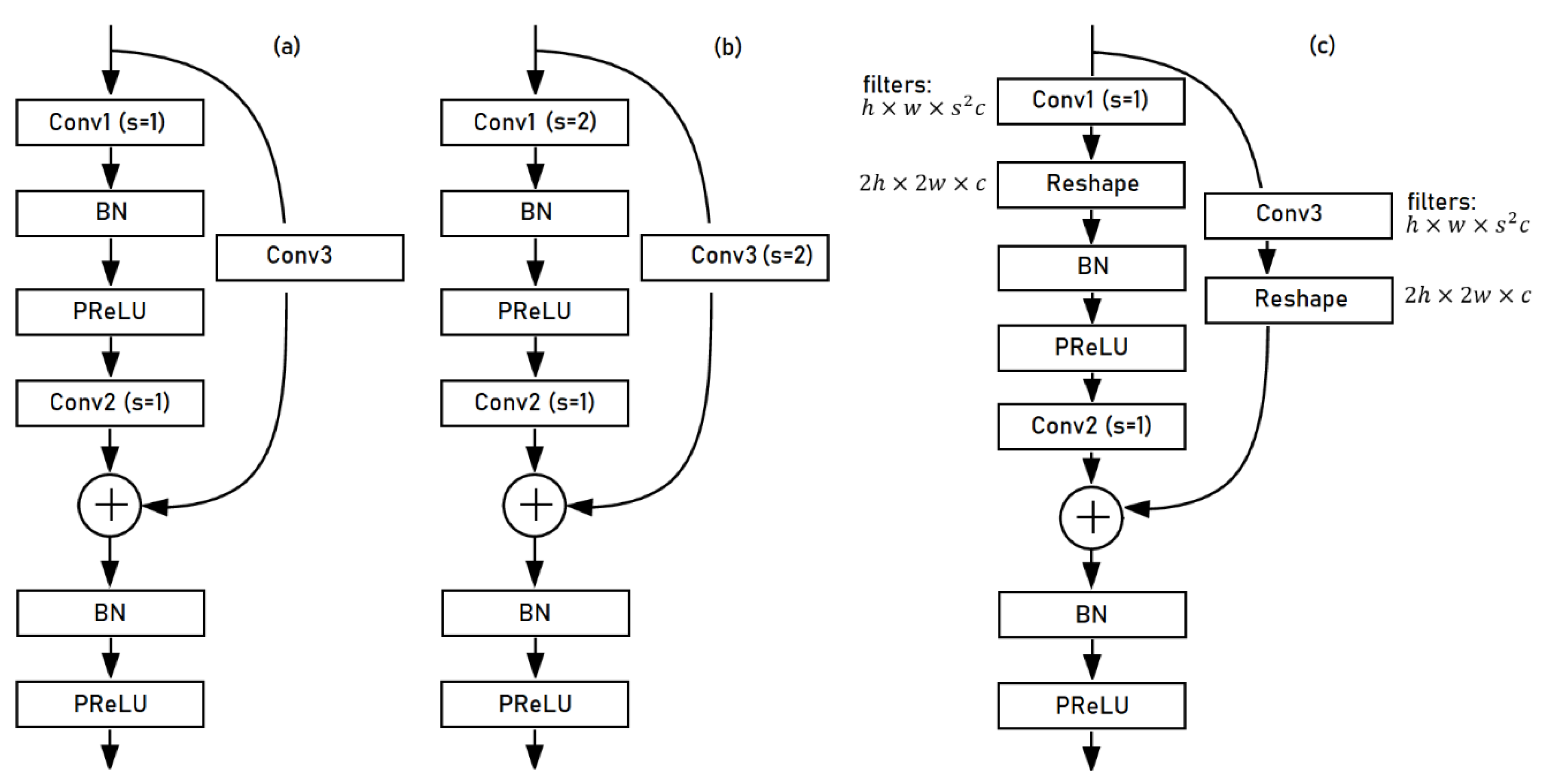
The U-Net architecture was implemented with residual blocks both in the encoder and the decoder mechanisms. Specifically, three types of residual blocks were used, as shown in Figure 4:
- a typical residual block (RBLK),
- a down-sampling residual block (DRBLK) and
- an up-sampling residual block (URBLK).
A typical residual block contains two convolutional layers at the data path and a convolutional layer with a kernel size of one at the residual connection path. The down-sampling residual block differs in the stride used at the first convolutional layer and the skip connection. Using a higher stride at these convolutions, the previous feature maps were downscaled by a factor s (here, s = 2) at the first convolutional layer of the block and the skip connection, which resulted in smaller feature maps. The up-sampling residual block used subpixel convolutional upscaling [54] in the first layer of the block. Subpixel upscaling was performed in two steps, with the first step calculating a representation comprising feature maps of sizes h × w × s2c, where s was the upscaling factor, and h × w × c was the size of the input feature maps. The second step of the process applied a reshape operation on the feature maps and produced a representation containing feature maps of sizes 2h × 2w × c. The skip connection of the upscaling residual block also applied subpixel upscaling. The detailed architecture of the residual blocks is shown in Figure 4.
A very similar model for both datasets was used, with minor changes regarding the input patch size and the size of the output prediction. The Manchester area dataset had an RGB image over a nDSM resolution ratio equal to 4, so the neural network dealing with this dataset reduced the input size from 256 × 256 × 4 to an output size of 64 × 64. On the other hand, the DFC2018 dataset had an RGB image over the depth map resolution ratio equal to 10, so the neural network dealing with this dataset reduced the input size from 520 × 520 × 4 to output size 52 × 52.
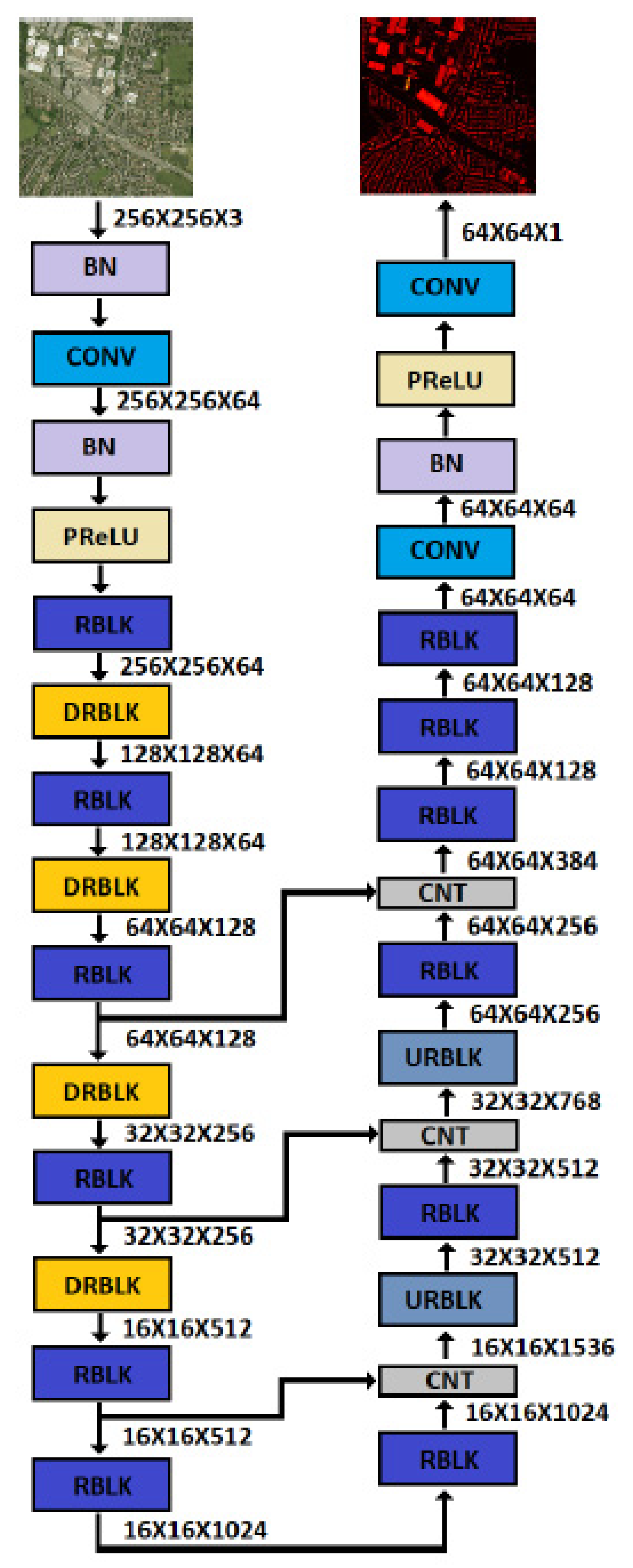
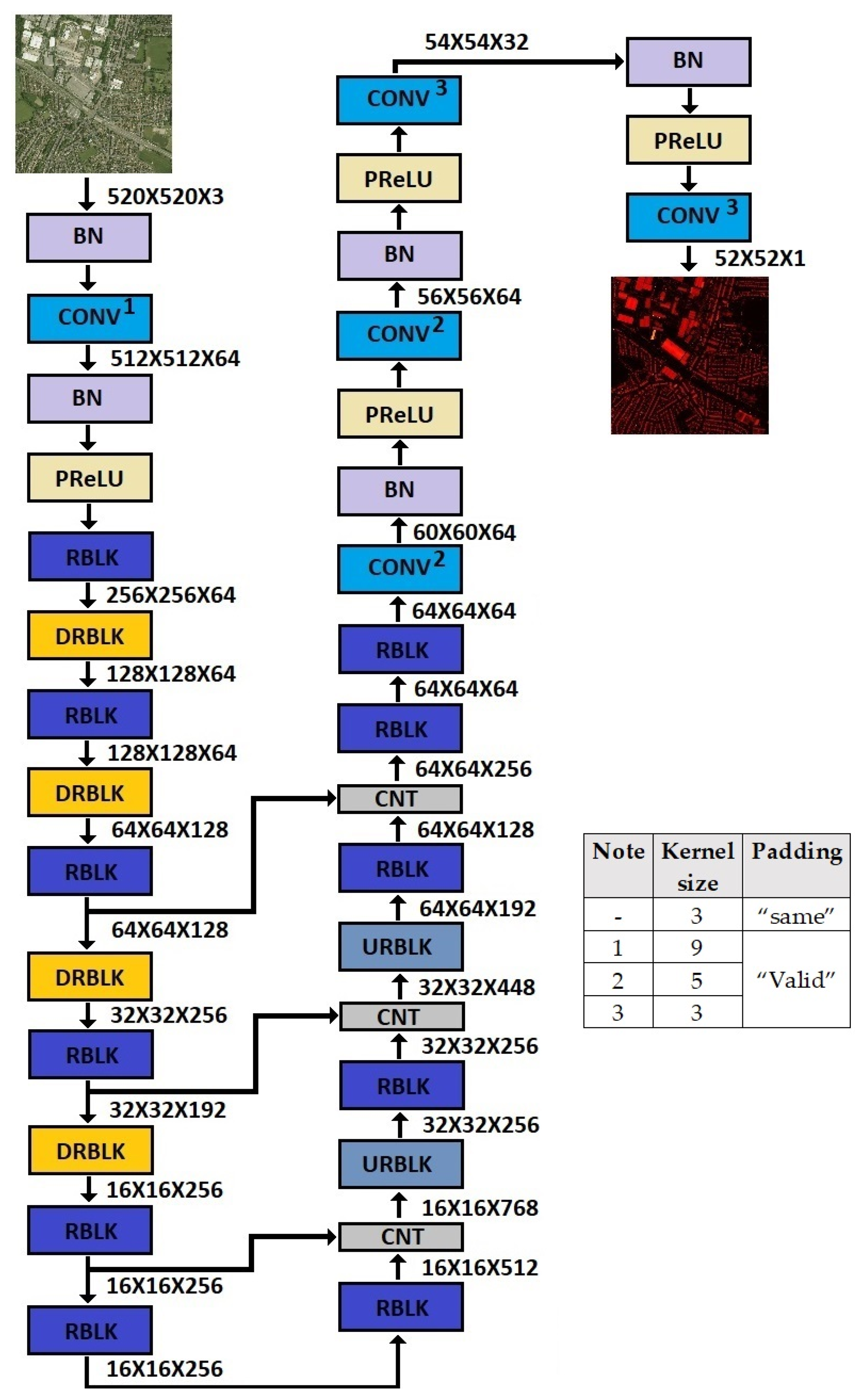
The input/output sizes of the models are a compromise between having a manageable input size in terms of the computational requirements and having a sufficient output map size and performance. The few differences between the two models are necessary for applying different reduction factors between the input and the output of the two datasets, as dictated by the RGB/nDSM resolution ratio of each dataset. Specifically, the number of layers, the number of channels and the kernel sizes of the convolutional layers of the model trained on the DFC2018 dataset were different from the ones used in the model trained on the Manchester dataset. This was due to the requirement of a larger resolution reduction. However, these changes were applied at the initial and the last layers of the model to maintain the U-NET scheme unaltered. Figure 5 and Figure 6 show the detailed architectures of both models and the sizes of the feature maps after each layer.
The model dealing with the Manchester area dataset had 164 layers (including concatenation layers and residual block addition layers) and consisted of approximately 125 million trainable parameters. The model dealing with the DFC2018 dataset had 186 layers (including concatenation layers and residual block addition layers) but had fewer parameters to handle the higher memory requirements during training due to the larger input size. Precisely, it consisted of 104 million trainable parameters. The only differences with the model used for the Manchester area dataset were (a) the addition of some convolutional layers with “valid” padding to achieve the correct output size and (b) the reduction of the parameters of the convolutional layers.
2.4. Training Details
Simple augmentations were applied to the patches during training: rotations of 90, 180 and 270 degrees; small-value color shifting and contrast variations. Patches where the elevation maps contained incomplete or extreme elevation values (>100 m) were ignored in both datasets. Moreover, specifically for the Manchester area dataset, small elevation values (<1.5 m) were replaced with zeros to prevent the model from considering nonstationary objects and low vegetation. This preprocessing is important in part because of the time difference between the acquisition of the RGB images and the LiDAR point clouds, which results in inconsistencies between the images and the elevation maps due to the presence of mobile objects like cars in the viewing field of either of the two sensors (RGB or LiDAR). The time of acquisition inconsistency in the Manchester area dataset also introduced inconsistencies in the vegetation height and, occasionally, in building heights (demolished buildings or newly constructed buildings). Consequently, regarding the Manchester area dataset, the model was focused on predicting the elevation of human-built structures like houses, factories and public buildings. The DFC2018 dataset had better resolution, and no inconsistencies were observed. This fact facilitated the prediction of the vegetation height as well; thus, a threshold filter was not applied to the ground truth nDSMs for the DFC2018 dataset.
The models were trained with the Adam optimizer [56] and a learning rate of 1 × 10⁻⁴, which decreased by a factor of 10 each time the error plateaued for several iterations. Both datasets were randomly split into three sets, each containing images of sizes 1000 × 1000 for the Manchester dataset and 5000 × 5000 for the DFC2018 dataset: a training set (70%), a validation set (15%) and a test set (15%). The validation set was used for hyperparameter fitting and then merged with the training set for retraining the models. The test set was only used to report the models’ performances. The models were trained for 5 different random dataset splits, and the average of the performances on the test sets was reported. The pixel-wise Mean Absolute Error (MAE) was used between the ground truth elevation maps and the predicted output as the loss function during training. The Mean Squared Error (MSE) was also considered, but it was found that the MAE performed slightly better, probably because it does not penalize outliers as much as the MSE. The Root Mean Squared Error (RMSE) performance was also reported as an additional evaluation metric. All parameters were initialized with the He normal technique [57].
3. Results
The model presented herein achieved a MAE of 0.59 m and an RMSE of 1.4 m for the Manchester area dataset, as well as a MAE of 0.78 m and an RMSE of 1.63 m for the DFC2018 dataset. The lower error values on the first dataset most likely occurred due to ignoring the small nDSM values (<1.5 m), increasing the model accuracy in the prediction of buildings and human-made structures. The proposed architecture improved on the results of Carvallo et al. [40] and Liu et al. [17] by a significant margin (see Table 1), although a direct comparison cannot be accurate, since all approaches use random data splits.
3.1. Height Prediction for the Manchester Area Dataset
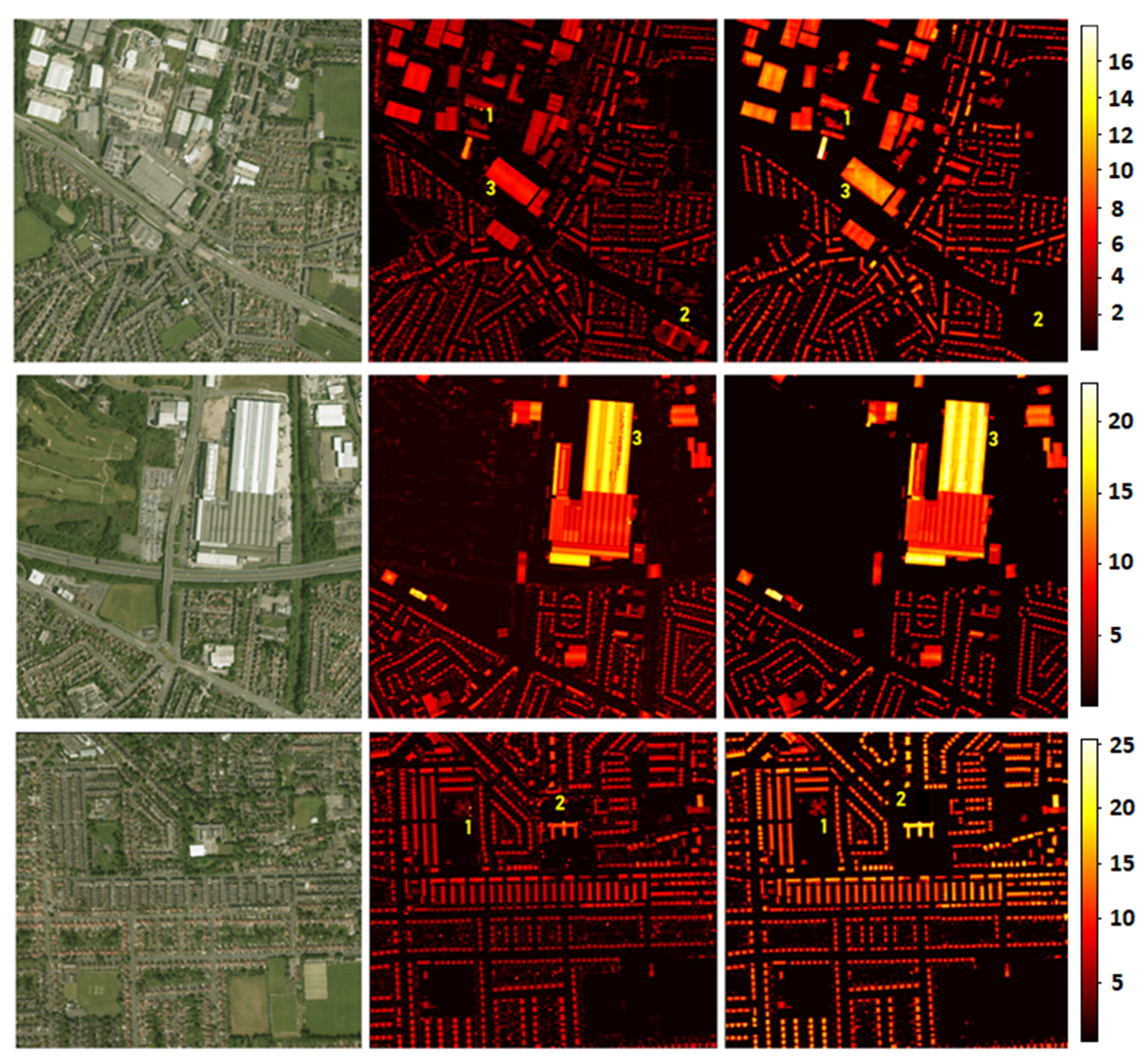
The estimated heights of areas in the Manchester Area test set are depicted in Figure 7. The estimations are shown in the form of heat maps for better visualization (i.e., providing a more precise display of the relative height values) and evaluation purposes. Since the model operates on patches of size 256 × 256 × 3, the RGB images were divided into several patches with overlapping regions of 16 pixels. Then, the model predicted a nDSM for each patch and, finally, the estimated maps were recombined to create the overall nDSM for the RGB image. During the recombination process, the outer 16 pixels of each predicted map were ignored to achieve a more natural blending and avoid artifacts.
Interestingly, the model avoided spiky estimations like the ones indicated with note 1 in the images of Figure 7: ground truth LiDAR maps occasionally contain points of unnaturally high values compared to neighboring points that constitute false readings that occur for several reasons. These reasons relate mainly to the physical properties of the LiDAR sensor and the environmental conditions during data acquisition (see Section 1 for a discussion on this). Furthermore, some incorrect readings may have values that lie in the boundary of reasonable LiDAR values and are difficult to discriminate from incomplete readings with irrational values. Such spiky readings naturally occurred in the training set as well. Nevertheless, the model was not affected by such inconsistencies in the training set, and its estimates corresponding to spiky measurements in the “ground truth” data were closer to the actual ground truth (see Figure 7, note 1).
Moreover, the Manchester Area dataset contains several inconsistencies in regard to structures that were missing either from the RGB images or from the nDSM due to different acquisition times between the two data types. Such inconsistencies are shown in Figure 7 (indicated as note 2): In these cases, some structures presented in the ground truth nDSM were missing from the RGB images; however, the model correctly predicted the corresponding regions containing the inconsistencies as undeveloped spaces. This behavior was, of course, desired and demonstrated effectively that the IMG2nDSM model presented herein was robust to false training instances. Furthermore, the results revealed some additional cases that indicated that the model was doing a good job estimating the heights of buildings, surpassing the quality of the ground truth map, notably with noisy data on specific structures with known forms. Note 3 in Figure 7 demonstrates such a case where the ground truth map seems noisy, given the known form of the apex roof structure, while the estimation of the model is more detailed and smoother. This raises the point that, although the model performance was calculated against the LiDAR data as the “ground truth”, it sometimes outperformed the LiDAR data and generated results closer to the actual ground truth.
3.2. Height Prediction for the DFC2018 Dataset
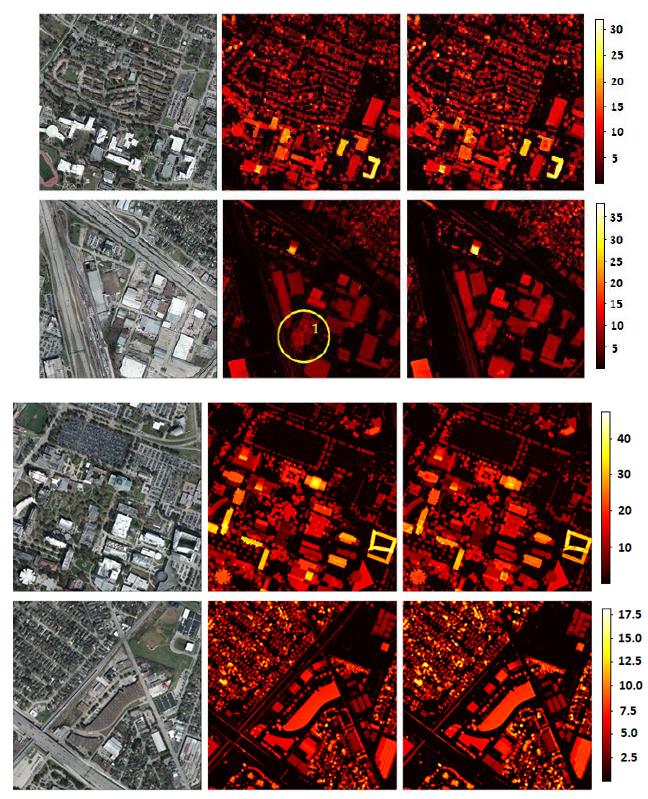
The estimated nDSMs of the consecutive areas of the DFC2018 test set are illustrated in Figure 8. As in the case of the Manchester Area test set, the RGB images were divided into overlapping patches, and the model predicted the nDSM for each of the patches. The only difference was that the size of the patches for this dataset was 520 × 520 × 3 pixels. The estimated nDSMs were fused together, as described in Section 3.1, to create the nDSM of the entire area.
The predicted nDSMs looked very similar to the ground truth. The higher resolution of the RGB images and the consistency between the RGB and the LiDAR measurements in terms of the data acquisition time had a positive impact on the model’s performance. For this dataset, the model could estimate the vegetation height accurately. Regarding vegetation, the model consistently overestimated the area covered by foliage, as it filled the space between the foliage. Note 1 in the second row of Figure 8 (located at the ground truth nDSM) shows the height measurements for a group of trees. Figure 9 shows the magnification of that area, the magnified ground truth map and the model’s height estimation and demonstrates the tendency of the model to overestimate the volume of foliage. It is thought that this behavior contributed to the higher MAE that the model scored on the DFC2018 dataset compared to the better performance on the Manchester area dataset. As described above, the latter dataset had a lower resolution and more inconsistencies, but the model training ignored the vegetation and low-standing objects to its favor. However, despite the associated higher MAE, this behavior of the model with a vegetation height estimation could be beneficial under some circumstances, such as projects that focus on tree counting, monitoring tree growth or tree coverage in an area [12].
3.3. Model Analysis
The very good results of the model, as shown in Table 1, result from its carefully designed architecture, which was selected after many experiments and trials with various alternate options. The initial form of the model was a basic model with the U-NET scheme proposed in reference [50] with typical residual blocks (Figure 4a) only, max-pooling (down-sampling) layers and nearest-neighbor interpolation (up-sampling) layers. Then, the basic model was improved upon by replacing individual architectural features with ones that improved the performance. The modifications that affected the performance the most are listed according to their contribution (higher contribution first):
- Use of the up-sampling residual block (URBLK), as shown in Figure 4c, instead of the nearest-neighbor interpolation.
- Use of the down-sampling residual block (DRBLK) with strided convolutions, as shown in Figure 4b, instead of max-pooling.
- Modification of the basic U-NET scheme so that the first two concatenation layers are applied before the up-sampling steps and not after them, as originally proposed in reference [50].
- Use of “same” instead of “valid” padding in the U-NET scheme.
- Replace the ReLU activation functions with PReLUs.
The first three modifications (the use of URBLKs and DRBLKs and the changes in the concatenation layers positions) enabled the model to surpass the performances of other state-of-the-art works, while the remaining modifications (the use of “same” padding and PReLUs) further increased the performance in favor of the proposed model, widening the gap. Overall, the proposed model relied on a task-specific architecture for achieving good results in predicting the nDSM of a scene from an aerial image.
3.4. Investigation of the Model’s Reliance on Shadows
The proposed DL models apply representation learning to discover the features needed to learn the task. Besides structural and scene geometry features, shadows are an important geometric cue, and they directly correlate with the height of the structures that cause them. Van Dijk et al. [58] reported that an object with shadow is more likely to be detected by a DL model trained for depth estimation than an object without a shadow. Christie et al. [59] cast shadows in each LiDAR map that matched the shadows observed in the RGB image to improve the reliability of image matching.
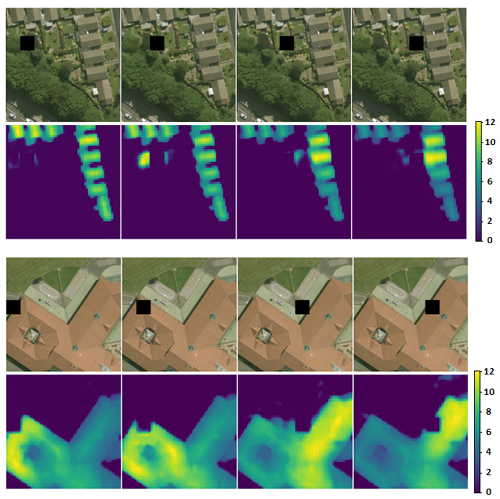
To investigate whether the model was indeed considering shadows for predicting the nDSMs, an experiment was conducted to observe how the model changed its prediction after the manipulation of shadows in the image patch. Specifically, a small square mask (window) was moved over the image patch, altering the values of the area under the mask. The sliding window set the underlying values to zero and, thus, simulated the presence of a shadow. The effect of this value adjustment on the model’s prediction was observed to significantly affect the nDSM prediction (see Figure 10). Shadow removal was also attempted by replacing dark shadow pixels in an image with higher values, but this did not influence the prediction as significantly as the shadow addition. This observation implies that the model has some prediction dependency on both the detection of the features of a structure and its associated shadow. Removing the shadow of a structure resulted in a slightly lower height prediction for the structure, but this did not fool the model into ignoring the shadowless building. In the other case, simulating a large shadow anywhere in the image caused the model to increase its elevation prediction for any evident object around that shadow. Figure 10 shows how the model’s prediction is affected by sliding a zero-value masking window over the RGB images. When the masking window adjoined the structures in the images, the model was driven into predicting larger height values for these structures. In the case that there were no structures adjoining the artificial shadow, the impact of the shadow manipulation was negligible.
In summary, the results of this experiment suggest that the model does consider shadows for computing the height of the structures in the RGB image, yet is not dependent on them. A shadow that is not associated with a nearby structure does not fool the model into predicting a building nearby. Thus, there is evidence that the model combines the presence of a shadow together with the features of an object to compute its height.
3.5. Limitations
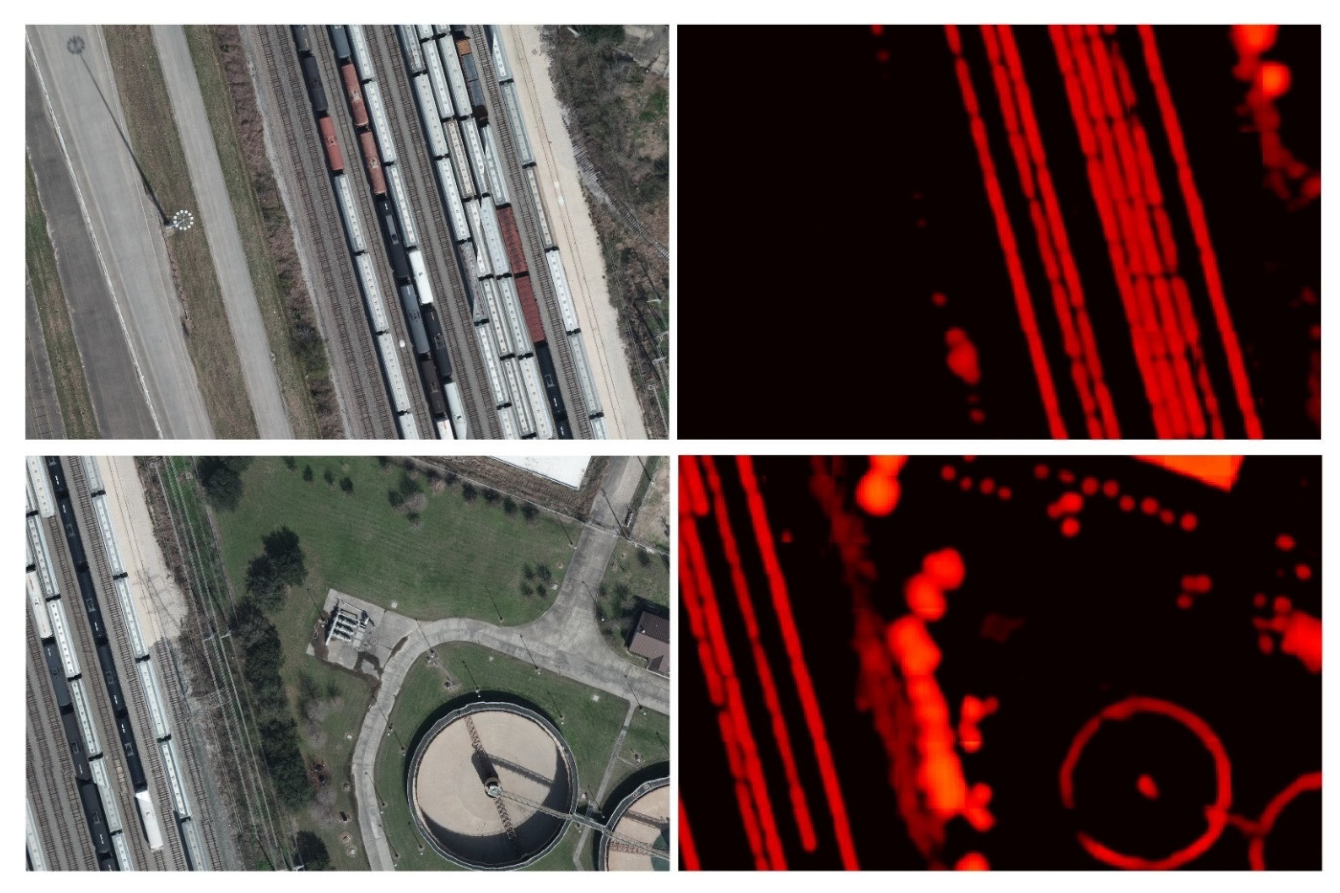
Despite the overall promising results of the proposed model, there were still some cases where the model did not perform correctly. Buildings were well-represented in both datasets, and thus, the model could predict their heights with little error. The same applied to vegetation in the DFC2018 dataset. However, for objects that were rarely seen in the data (e.g., objects that were tall and thin simultaneously, such as light poles and telecommunication towers), the model sometimes failed to estimate their heights correctly. In cases of very scarce objects, the model treated them as if they did not exist. Rarely seen tall objects that were not bulky or whose structure had empty interior spaces were tough for the model to assess. Examples of such failed cases are shown in Figure 11. The leading cause of the problem was is the under-representation of these structures in the dataset. This can be mitigated by introducing more images containing these objects during training.
Although the model performs well, it is acknowledged that it has many parameters. However, it is quite fast when predicting the nDSM of an individual patch, especially when the model runs on a Graphical Processing Unit (GPU). Inferring the nDSM of a large area requires the splitting of the RGB image into several patches. Using a GPU, the estimation of the nDSMs of all patches was performed in parallel by processing a batch (or batches) of patches, taking advantage of the hardware and its parallel computing capabilities.
4. Discussion
Obtaining the heights of objects in aerial photography with hardware equipment can be costly, time-consuming and require human expertise and sophisticated instruments. Furthermore, the acquisition techniques of such data are demanding and require specialized operators. On the other hand, inferring this data solely from aerial RGB images is easier, faster and especially helpful if the availability of image pairs is limited for a certain terrain modeling task. Height estimations from aerial imagery are difficult due to its ill-posed nature, yet DL techniques offer a promising perspective towards providing adequate solutions to the task.
The authors proposed a model, named IMG2nDSM, with a task-focused DL architecture that tackled the problem with very good results, which were better than the state-of-the-art ones to date. The model was tested on two different datasets: one with 0.25 m by 0.25 m image resolution, 1-m LiDAR resolution and different acquisition times (thus, it had spatial inconsistencies) and one with 0.05 m by 0.05 m image resolution and 0.5-m LiDAR resolution. The first dataset (capturing lower resolution images) covered the Trafford area in Manchester, UK, while the second dataset was part of the 2018 IEEE GRSS Data Fusion Contest. The first dataset was used to estimate building heights only, while the second dataset was used to estimate both buildings and vegetation heights. Despite the inconsistencies encountered in the first dataset, the effectiveness of the model indicated its high robustness and ability to build domain knowledge without resorting to dataset memorization. This indication was also suggested by the fact that data curation or special prepossessing, besides data augmentation, was not employed.
The authors aspired to the idea that the possibility of deriving high-precision digital elevation models from RGB images without expensive equipment and high costs will accelerate global efforts in various application domains that require the geometric analysis of areas and scenes. Such domains include urban planning and digital twins for smart cities [11], tree growth monitoring and forest mapping [12], modeling ecological and hydrological dynamics [60], detecting farmland infrastructures [61], etc. Such low-cost estimations of building heights will allow policymakers to understand the potential revenue of rooftop photovoltaics based on the yearly access to sunshine [62] and law enforcement to verify whether urban/or rural infrastructures comply with the local land registry legislation.
Finally, it is noted that the model experienced some cases of poor performance with tall and thin and generally under-represented objects. This issue can be solved by including more examples of such objects in the training images, which is an aspect of future works.
5. Conclusions
A DL model, IMG2nDSM, was proposed for inferring the heights of objects in single aerial RGB images. The model was trained with aerial images and their corresponding nDSMs acquired from LiDAR point clouds, but only the RGB images were required during the inference. The model was tested on two datasets, and its performance was significantly better than the other state-of-the-art methods. The results proved that the model built good domain knowledge and sometimes produced results that were better compared to the LiDAR data when assessing the ground truth scenario. The model’s behavior regarding vegetation height estimations was also analyzed, and some failed cases were reported.
Future research directions and model improvements include the reduction of failed cases for under-represented structures in aerial imagery, such as rarely seen special-purpose structures with electronic devices, telecommunication towers and energy transmission towers. The value of the proposed methodology stems from its convenient and easy application and the fact that it only requires RGB images during inference. Achieving the height estimation task from single RGB images without requiring LiDAR or any other information greatly reduces the cost, required effort and time and the difficulties that emerge from using complex data acquisition techniques or complex analytical computations.
Author Contributions
Conceptualization, S.K. and A.K.; methodology, S.K.; software, S.K.; validation, S.K.; formal analysis, S.K.; investigation, S.K.; resources, S.K., I.C.; data curation, S.K. and I.C.; writing—original draft preparation, S.K.; writing—review and editing, A.K. and I.C.; visualization, S.K.; supervision, A.K. and project administration, A.K. All authors have read and agreed to the published version of the manuscript.
Funding
This project received funding from the European Union’s Horizon 2020 Research and Innovation Programme under Grant Agreement No. 739578 and the Government of the Republic of Cyprus through the Deputy Ministry of Research, Innovation and Digital Policy.
Acknowledgments
The authors thank Chirag Prabhakar Padubidri for his consulting on handling the DFC2018 dataset.
Conflicts of Interest
The authors declare no conflict of interest.
References
- Wellmann, T.; Lausch, A.; Andersson, E.; Knapp, S.; Cortinovis, C.; Jache, J.; Scheuer, S.; Kremer, P.; Mascarenhas, A.; Kraemer, R.; et al. Remote Sensing in Urban Planning: Contributions towards Ecologically Sound Policies? Landsc. Urban Plan. 2020, 204, 103921. [Google Scholar] [CrossRef]
- Bechtel, B. Recent Advances in Thermal Remote Sensing for Urban Planning and Management. In Proceedings of the Joint Urban Remote Sensing Event, JURSE 2015, Lausanne, Switzerland, 30 March–1 April 2015; IEEE: Piscataway, NJ, USA, 2015; pp. 1–4. [Google Scholar]
- Zhu, Z.; Zhou, Y.; Seto, K.C.; Stokes, E.C.; Deng, C.; Pickett, S.T.A.; Taubenböck, H. Understanding an Urbanizing Planet: Strategic Directions for Remote Sensing. Remote Sens. Environ. 2019, 228, 164–182. [Google Scholar] [CrossRef]
- Lesiv, M.; Schepaschenko, D.; Moltchanova, E.; Bun, R.; Dürauer, M.; Prishchepov, A.V.; Schierhorn, F.; Estel, S.; Kuemmerle, T.; Alcántara, C.; et al. Spatial Distribution of Arable and Abandoned Land across Former Soviet Union Countries. Sci. Data 2018, 5, 1–12. [Google Scholar] [CrossRef]
- Ma, L.; Li, M.; Blaschke, T.; Ma, X.; Tiede, D.; Cheng, L.; Chen, Z.; Chen, D. Object-Based Change Detection in Urban Areas: The Effects of Segmentation Strategy, Scale, and Feature Space on Unsupervised Methods. Remote Sens. 2016, 8, 761. [Google Scholar] [CrossRef] [Green Version]
- Muro, J.; Canty, M.; Conradsen, K.; Hüttich, C.; Nielsen, A.A.; Skriver, H.; Remy, F.; Strauch, A.; Thonfeld, F.; Menz, G. Short-Term Change Detection in Wetlands Using Sentinel-1 Time Series. Remote Sens. 2016, 8, 795. [Google Scholar] [CrossRef] [Green Version]
- Lyu, H.; Lu, H.; Mou, L. Learning a Transferable Change Rule from a Recurrent Neural Network for Land Cover Change Detection. Remote Sens. 2016, 8, 506. [Google Scholar] [CrossRef] [Green Version]
- Kaku, K. Satellite Remote Sensing for Disaster Management Support: A Holistic and Staged Approach Based on Case Studies in Sentinel Asia. Int. J. Disaster Risk Reduct. 2019, 33, 417–432. [Google Scholar] [CrossRef]
- Wing, M.G.; Burnett, J.; Sessions, J.; Brungardt, J.; Cordell, V.; Dobler, D.; Wilson, D. Eyes in the Sky: Remote Sensing Technology Development Using Small Unmanned Aircraft Systems. J. For. 2013, 111, 341–347. [Google Scholar] [CrossRef]
- Mulac, B.L. Remote Sensing Applications of Unmanned Aircraft: Challenges to Flight in United States Airspace. Geocarto Int. 2011, 26, 71–83. [Google Scholar] [CrossRef]
- Xue, F.; Lu, W.; Chen, Z.; Webster, C.J. From LiDAR Point Cloud towards Digital Twin City: Clustering City Objects Based on Gestalt Principles. ISPRS J. Photogramm. Remote Sens. 2020, 167, 418–431. [Google Scholar] [CrossRef]
- Michałowska, M.; Rapiński, J. A Review of Tree Species Classification Based on Airborne LiDAR Data and Applied Classifiers. Remote Sens. 2021, 13, 353. [Google Scholar] [CrossRef]
- Schönberger, J.L.; Frahm, J.-M. Structure-from-Motion Revisited. In Proceedings of the 2016 IEEE Conference on Computer Vision and Pattern Recognition, CVPR 2016, Las Vegas, NV, USA, 27–30 June 2016; IEEE Computer Society: Washington, DC, USA, 2016; pp. 4104–4113. [Google Scholar]
- Bosch, M.; Foster, K.; Christie, G.A.; Wang, S.; Hager, G.D.; Brown, M.Z. Semantic Stereo for Incidental Satellite Images. In Proceedings of the IEEE Winter Conference on Applications of Computer Vision, WACV 2019, Waikoloa Village, HI, USA, 7–11 January 2019; IEEE: Picataway, NJ, USA, 2019; pp. 1524–1532. [Google Scholar]
- Voumard, J.; Derron, M.-H.; Jaboyedoff, M.; Bornemann, P.; Malet, J.-P. Pros and Cons of Structure for Motion Embarked on a Vehicle to Survey Slopes along Transportation Lines Using 3D Georeferenced and Coloured Point Clouds. Remote Sens. 2018, 10, 1732. [Google Scholar] [CrossRef] [Green Version]
- Liu, X. Airborne LiDAR for DEM Generation: Some Critical Issues. Prog. Phys. Geogr. Earth Environ. 2008, 32, 31–49. [Google Scholar]
- Liu, C.-J.; Krylov, V.A.; Kane, P.; Kavanagh, G.; Dahyot, R. IM2ELEVATION: Building Height Estimation from Single-View Aerial Imagery. Remote Sens. 2020, 12, 2719. [Google Scholar] [CrossRef]
- He, K.; Gkioxari, G.; Dollár, P.; Girshick, R.B. Mask R-CNN. IEEE Trans. Pattern Anal. Mach. Intell. 2020, 42, 386–397. [Google Scholar] [CrossRef] [PubMed]
- Chen, L.-C.; Papandreou, G.; Schroff, F.; Adam, H. Rethinking Atrous Convolution for Semantic Image Segmentation. arXiv 2017, arXiv:1706.05587. [Google Scholar]
- Güler, R.A.; Neverova, N.; Kokkinos, I. DensePose: Dense Human Pose Estimation in the Wild. In Proceedings of the 2018 IEEE Conference on Computer Vision and Pattern Recognition, CVPR 2018, Salt Lake City, UT, USA, 18–22 June 2018; IEEE Computer Society: Washington, DC, USA, 2018; pp. 7297–7306. [Google Scholar]
- Szegedy, C.; Vanhoucke, V.; Ioffe, S.; Shlens, J.; Wojna, Z. Rethinking the Inception Architecture for Computer Vision. In Proceedings of the 2016 IEEE Conference on Computer Vision and Pattern Recognition, CVPR 2016, Las Vegas, NV, USA, 27–30 June 2016; IEEE Computer Society: Washington, DC, USA, 2016; pp. 2818–2826. [Google Scholar]
- He, K.; Zhang, X.; Ren, S.; Sun, J. Deep Residual Learning for Image Recognition. In Proceedings of the Conference on Computer Vision and Pattern Recognition (CVPR) 2016, Las Vegas, NV, USA, 27–30 June 2016; pp. 770–778. [Google Scholar]
- Krizhevsky, A.; Sutskever, I.; Geoffrey, E.H. ImageNet Classification with Deep Convolutional Neural Networks. In Proceedings of the Advances in Neural Information Processing Systems (NIPS), Lake Tahoe, NV, USA, 3–6 December 2012; Pereira, F., Burges, C.J.C., Bottou, L., Weinberger, K.Q., Eds.; Curran Associates, Inc.: Brooklyn, NY, USA, 2012; pp. 1097–1105. [Google Scholar]
- Tan, C.; Sun, F.; Kong, T.; Zhang, W.; Yang, C.; Liu, C. A Survey on Deep Transfer Learning. In Proceedings of the Artificial Neural Networks and Machine Learning—CANN 2018—27th International Conference on Artificial Neural Networks, Rhodes, Greece, 4–7 October 2018; Proceedings, Part III. Kurková, V., Manolopoulos, Y., Hammer, B., Iliadis, L.S., Maglogiannis, I., Eds.; Springer: New York, NY, USA, 2018; Volume 11141, pp. 270–279. [Google Scholar]
- Eigen, D.; Puhrsch, C.; Fergus, R. Depth Map Prediction from a Single Image Using a Multi-Scale Deep Network. In Proceedings of the Advances in Neural Information Processing Systems 27: Annual Conference on Neural Information Processing Systems 2014, Montreal, QC, Canada, 8–13 December 2014; Ghahramani, Z., Welling, M., Cortes, C., Lawrence, N.D., Weinberger, K.Q., Eds.; Red Hook: New York, NY, USA, 2014; pp. 2366–2374. [Google Scholar]
- Laina, I.; Rupprecht, C.; Belagiannis, V.; Tombari, F.; Navab, N. Deeper Depth Prediction with Fully Convolutional Residual Networks. arXiv 2016, arXiv:1606.00373. [Google Scholar]
- Alhashim, I.; Wonka, P. High Quality Monocular Depth Estimation via Transfer Learning. arXiv 2018, arXiv:1812.11941. [Google Scholar]
- Huang, G.; Liu, Z.; Weinberger, K.Q. Densely Connected Convolutional Networks. CoRR 2016. [Google Scholar]
- Deng, J.; Dong, W.; Socher, R.; Li, L.-J.; Li, K.; Fei-Fei, L. Imagenet: A Large-Scale Hierarchical Image Database. In Proceedings of the 2009 IEEE Conference on Computer Vision and Pattern Recognition, Miami, FL, USA, 20–25 June 2009; pp. 248–255. [Google Scholar]
- Bhat, S.F.; Alhashim, I.; Wonka, P. AdaBins: Depth Estimation Using Adaptive Bins. arXiv 2020, arXiv:2011.14141. [Google Scholar]
- Geiger, A.; Lenz, P.; Urtasun, R. Are We Ready for Autonomous Driving? The KITTI Vision Benchmark Suite. In Proceedings of the Conference on Computer Vision and Pattern Recognition (CVPR), Providence, RI, USA, 16–21 June 2012. [Google Scholar]
- Nathan Silberman Derek Hoiem, P.K.; Fergus, R. Indoor Segmentation and Support Inference from RGBD Images. In Proceedings of the ECCV, Florence, Italy, 7–13 October 2012. [Google Scholar]
- Mahjourian, R.; Wicke, M.; Angelova, A. Unsupervised Learning of Depth and Ego-Motion From Monocular Video Using 3D Geometric Constraints. In Proceedings of the 2018 IEEE Conference on Computer Vision and Pattern Recognition, CVPR 2018, Salt Lake City, UT, USA, 18–22 June 2018; IEEE Computer Society: Washington, DC, USA, 2018; pp. 5667–5675. [Google Scholar]
- PNVR, K.; Zhou, H.; Jacobs, D. SharinGAN: Combining Synthetic and Real Data for Unsupervised Geometry Estimation. In Proceedings of the 2020 IEEE/CVF Conference on Computer Vision and Pattern Recognition, CVPR 2020, Seattle, WA, USA, 13–19 June 2020; IEEE: Picataway, NJ, USA, 2020; pp. 13971–13980. [Google Scholar]
- Goodfellow, I.; Pouget-Abadie, J.; Mirza, M. Generative Adversarial Networks. arXiv 2014, arXiv:1406.2661. [Google Scholar] [CrossRef]
- Yu, D.; Ji, S.; Liu, J.; Wei, S. Automatic 3D Building Reconstruction from Multi-View Aerial Images with Deep Learning. ISPRS J. Photogramm. Remote Sens. 2021, 171, 155–170. [Google Scholar] [CrossRef]
- Mou, L.; Zhu, X.X. IM2HEIGHT: Height Estimation from Single Monocular Imagery via Fully Residual Convolutional-Deconvolutional Network. arXiv 2018, arXiv:1802.10249. [Google Scholar]
- Amirkolaee, H.A.; Arefi, H. Height Estimation from Single Aerial Images Using a Deep Convolutional Encoder-Decoder Network. ISPRS J. Photogramm. Remote Sens. 2019, 149, 50–66. [Google Scholar] [CrossRef]
- Srivastava, S.; Volpi, M.; Tuia, D. Joint Height Estimation and Semantic Labeling of Monocular Aerial Images with CNNS. In Proceedings of the 2017 IEEE International Geoscience and Remote Sensing Symposium, IGARSS 2017, Fort Worth, TX, USA, 23–28 July 2017; IEEE: Picataway, NJ, USA, 2017; pp. 5173–5176. [Google Scholar]
- Carvalho, M.; Le Saux, B.; Trouvé-Peloux, P.; Champagnat, F.; Almansa, A. Multitask Learning of Height and Semantics From Aerial Images. IEEE Geosci. Remote. Sens. Lett. 2020, 17, 1391–1395. [Google Scholar] [CrossRef] [Green Version]
- Ghamisi, P.; Yokoya, N. IMG2DSM: Height Simulation from Single Imagery Using Conditional Generative Adversarial Net. IEEE Geosci. Remote Sens. Lett. 2018, 15, 794–798. [Google Scholar] [CrossRef]
- Panagiotou, E.; Chochlakis, G.; Grammatikopoulos, L.; Charou, E. Generating Elevation Surface from a Single RGB Remotely Sensed Image Using Deep Learning. Remote Sens. 2020, 12, 2002. [Google Scholar] [CrossRef]
- Goodfellow, I.; Bengio, Y.; Courville, A. Deep Learning; MIT Press: Cambridge, MA, USA, 2016; ISBN 9780874216561. [Google Scholar]
- Nielsen, M. Neural Networks and Deep Learning. Available online: http://neuralnetworksanddeeplearning.com/ (accessed on 24 March 2021).
- Digimap. Available online: https://0-digimap-edina-ac-uk.brum.beds.ac.uk/ (accessed on 25 March 2021).
- Edina. Available online: https://0-edina-ac-uk.brum.beds.ac.uk/ (accessed on 25 March 2021).
- Defra (Department for Environment, Food and Rural Affairs). Spatial Data. Available online: https://environment.data.gov.uk/DefraDataDownload/ (accessed on 25 March 2021).
- 2018 IEEE GRSS Data Fusion Contest. Available online: http://dase.grss-ieee.org/index.php (accessed on 24 March 2021).
- IEEE. France GRSS Chapter. Available online: https://0-site-ieee-org.brum.beds.ac.uk/france-grss/2018/01/16/data-fusion-contest-2018-contest-open/ (accessed on 24 March 2021).
- Ronneberger, O.; Fischer, P.; Brox, T. U-Net: Convolutional Networks for Biomedical Image Segmentation. In Proceedings of the International Conference of Medical Image Computing and Computer-Assisted Intervention 18 (MICCAI), Munich, Germany, 5–9 October 2015; pp. 234–241. [Google Scholar]
- Çiçek, Ö.; Abdulkadir, A.; Lienkamp, S.S.; Brox, T.; Ronneberger, O. 3D U-Net: Learning Dense Volumetric Segmentation from Sparse Annotation. In Proceedings of the Medical Image Computing and Computer-Assisted Intervention (MICCAI), Athens, Greece, 17–21 October 2016; Ourselin, S., Joskowicz, L., Sabuncu, M.R., Ünal, G.B., Wells, W., Eds.; Springer: New York, NY, USA, 2016; Volume 9901, pp. 424–432. [Google Scholar]
- Iglovikov, V.; Shvets, A. TernausNet: U-Net with VGG11 Encoder Pre-Trained on ImageNet for Image Segmentation. arXiv 2018, arXiv:1801.05746. [Google Scholar]
- Long, J.; Shelhamer, E.; Darrell, T. Fully Convolutional Networks for Semantic Segmentation. In Proceedings of the IEEE Conference on Computer Vision and Pattern Recognition, CVPR 2015, Boston, MA, USA, 7–12 June 2015; pp. 3431–3440. [Google Scholar]
- Shi, W.; Caballero, J.; Huszar, F.; Totz, J.; Aitken, A.P.; Bishop, R.; Rueckert, D.; Wang, Z. Real-Time Single Image and Video Super-Resolution Using an Efficient Sub-Pixel Convolutional Neural Network. In Proceedings of the 2016 IEEE Conference on Computer Vision and Pattern Recognition, CVPR 2016, Las Vegas, NV, USA, 27–30 June 2016; IEEE Computer Society: Washington, DC, USA, 2016; pp. 1874–1883. [Google Scholar]
- Ioffe, S.; Szegedy, C. Batch Normalization: Accelerating Deep Network Training by Reducing Internal Covariate Shift. arXiv 2015, arXiv:1502.03167. [Google Scholar]
- Kingma, D.P.; Ba, J. Adam: A Method for Stochastic Optimization. ICLR 2015, 1–15. [Google Scholar] [CrossRef]
- He, K.; Zhang, X.; Ren, S.; Sun, J. Delving Deep into Rectifiers: Surpassing Human-Level Performance on ImageNet Classification. In Proceedings of the International Conference on Computer Vision (ICCV), Santiago, Chile, 7–13 December 2015; pp. 1026–1034. [Google Scholar]
- Van Dijk, T.; de Croon, G. How Do Neural Networks See Depth in Single Images? In Proceedings of the International Conference on Computer Vision, Seoul, Korea, 27 October–2 November 2019; IEEE: Picataway, NJ, USA, 2019; pp. 2183–2191. [Google Scholar]
- Christie, G.A.; Abujder, R.R.R.M.; Foster, K.; Hagstrom, S.; Hager, G.D.; Brown, M.Z. Learning Geocentric Object Pose in Oblique Monocular Images. In Proceedings of the Conference on Computer Vision and Pattern Recognition, CVPR 2020, Seattle, WA, USA, 13–19 June 2020; IEEE: Picataway, NJ, USA, 2020; pp. 14500–14508. [Google Scholar]
- Jones, K.L.; Poole, G.C.; O’Daniel, S.J.; Mertes, L.A.K.; Stanford, J.A. Surface Hydrology of Low-Relief Landscapes: Assessing Surface Water Flow Impedance Using LIDAR-Derived Digital Elevation Models. Remote Sens. Environ. 2008, 112, 4148–4158. [Google Scholar] [CrossRef]
- Sofia, G.; Bailly, J.; Chehata, N.; Tarolli, P.; Levavasseur, F. Comparison of Pleiades and LiDAR Digital Elevation Models for Terraces Detection in Farmlands. IEEE J. Sel. Top. Appl. Earth Obs. Remote Sens. 2016, 9, 1567–1576. [Google Scholar] [CrossRef] [Green Version]
- Palmer, D.; Koumpli, E.; Cole, I.; Gottschalg, R.; Betts, T. A GIS-Based Method for Identification of Wide Area Rooftop Suitability for Minimum Size PV Systems Using LiDAR Data and Photogrammetry. Energies 2018, 11, 3506. [Google Scholar] [CrossRef] [Green Version]
Figure 1.
Aerial images from the first dataset (left), the corresponding nDSMs in heat map format and their color bars, indicating the color-coding of the nDSM in meters (right). The aerial images on the left of each pair have a size of 4000 × 4000, while the size of the nDSMs is 1000 × 1000. nDSMs are presented at the same size as the aerial images for demonstration reasons. The Figure is best seen in color.

Figure 2.
The DSM (left) and the DTM (right) corresponding to the bottom aerial image of Figure 1. The color bar for each heat map indicates the color-coding of the DEMs in meters above sea level. Both heat maps have several undetermined or irrational (extremely high or low) values shown in black color. Notably, some of these unexpected values in the DSM map (left) correspond to a river, which illustrates a well-known problem of LiDAR measurements near highly reflective and refractive surfaces with multiple light paths. Such erroneous values raise significant problems regarding the training of the model. Thus, they are detected during data preprocessing and excluded from the training data (see Section 2.4). They are also excluded from the validation and test data to avoid inaccurate performance evaluations. Overall, these values roughly comprise 10% of the dataset but lead to a larger amount of discarded data, since any candidate patch containing even a pixel of undetermined or irrational value is excluded from the training pipeline. This figure is best seen in color.

Figure 3.
Aerial images from the IEEE GRSS Data Fusion Contest (second dataset), the corresponding nDSMs and the color bars of the heat maps indicating the color-coding in meters. The RGB images on the left of each pair have a size of 5000 × 5000 pixels, while the size of the nDSMs is 500 × 500 pixels. The heat maps are shown as the same size as the aerial images for demonstration reasons. This figure is best seen in color.

Figure 4.
The architecture of the three types of residual blocks used in the proposed models: (a) the typical residual block (RBLK). (b) The down-sampling residual block (DRBLK) uses a stride of two at both the first convolutional layer and the skip connection. (c) The up-sampling residual block (URBLK) uses subpixel upscaling at the first convolution and the skip connection. BN stands for batch normalization [55], PReLU for parametric ReLU and s is the stride of the convolutional layer.

Figure 5.
The architecture of the model trained with the Manchester dataset. All convolutional layers use kernel size 3 and “same” padding. BN represents a Batch Normalization layer and CNT a Concatenation layer.
Figure 5.
The architecture of the model trained with the Manchester dataset. All convolutional layers use kernel size 3 and “same” padding. BN represents a Batch Normalization layer and CNT a Concatenation layer.

Figure 6.
The architecture of the model trained with the DFC2018 dataset. Compared to the model trained with the Manchester dataset, the kernel sizes of certain convolutional layers are increased, and their padding is changed from “same” to “valid”, as indicated by the figure notes. Additionally, some convolutional layers are introduced at the end of the model. These modifications aim at applying a reduction factor of 10 between the input and the output of the model to match the resolution ratio between the aerial images and the nDSMs in the DFC2018 dataset. BN represents a Batch Normalization layer and CNT a Concatenation layer.

Figure 7.
Left: RGB images of an area in the test set of the Manchester area dataset. Middle: The ground truth nDSMs. Right: The elevation heat maps as predicted by the model. Note 1 shows cases of spurious points in the ground truth that the model correctly avoids estimating. Note 2 shows occasional inconsistencies in the dataset due to the different acquisition times of the RGB images and the LiDAR measurements. Although these inconsistencies are also evident in the training set, the model is robust to such problematic training instances. Note 3 shows cases where the model produces better-quality maps than the ground truth in terms of the surface smoothness and level of detail, as the LiDAR data contains noisy values.

Figure 8.
Left: RGB images from the DFC2018 test set. Middle: Ground truth nDSMs. Right: Model’s height estimations. Note 1 indicates an area that contains a group of trees and is magnified in Figure 9 to demonstrate how the model treats vegetation in the RGB images.
Figure 8.
Left: RGB images from the DFC2018 test set. Middle: Ground truth nDSMs. Right: Model’s height estimations. Note 1 indicates an area that contains a group of trees and is magnified in Figure 9 to demonstrate how the model treats vegetation in the RGB images.

Figure 9.
Magnification of the noted region (Note 1) in Figure 8. Left: The magnified RGB image. Middle: The ground truth nDSM. Right: Model output. The model consistently overestimates the foliage volume by filling the spaces between foliage with similar values to the neighboring estimations.
Figure 9.
Magnification of the noted region (Note 1) in Figure 8. Left: The magnified RGB image. Middle: The ground truth nDSM. Right: Model output. The model consistently overestimates the foliage volume by filling the spaces between foliage with similar values to the neighboring estimations.

Figure 10.
Using a sliding window to investigate whether the model uses shadows for object height estimation. Each test case is presented in pairs of consecutive rows, the upper row showing the RGB image with the position of the sliding masking window (black square) and the lower row the prediction at the model output. The artificial shadow implied by the square black box influences the height estimation of the buildings close to the shadow by increasing their height predictions (the values on the predicted map corresponding to the buildings that are close to the shadow are seen to be brighter in the image and, thus, higher in value). The estimated heights of buildings that are not near the implied shadow are not affected. The artificial shadow causes the model to predict a higher elevation for buildings that are in the shadow’s proximity. This figure is better seen in color.

Figure 11.
Sample failed cases where the model misses the presence of an object completely. The cases are magnified regions from the second RGB image (second row) of Figure 8. The top-left image shows a very high pole standing on a highway (on the left of the train wagons) with a height of 30 m (according to its LiDAR measurement). Despite the pole’s long shadow, the model does not detect it. The bottom-left magnified region contains a tall electric energy transmission tower (close and on the right of the train wagons) that is also not detected by the model.


Table 1.
Model’s performances on the test set and comparisons to other methods.
| Method | MAE(m) ↓ | RMSE(m) ↓ |
|---|---|---|
| Manchester Area dataset 1 | ||
| IMG2nDSM * | 0.59 | 1.4 |
| DFC2018 dataset 2 | ||
| Carvallo et al. [40] (DSM) | 1.47 | 3.05 |
| Carvallo et al. [40] (DSM + semantic) | 1.26 | 2.60 |
| Liu et al. [17] | 1.19 | 2.88 |
| IMG2nDSM * | 0.78 | 1.63 |
1 A 0.25-m/pixel RGB resolution, 1-m/pixel LiDAR resolution, inconsistencies. 2 A 0.05-m/pixel RGB resolution, 0.5-m/pixel LiDAR resolution. * IMG2nDSM is the model presented in this work.
Publisher’s Note: MDPI stays neutral with regard to jurisdictional claims in published maps and institutional affiliations. |
© 2021 by the authors. Licensee MDPI, Basel, Switzerland. This article is an open access article distributed under the terms and conditions of the Creative Commons Attribution (CC BY) license (https://creativecommons.org/licenses/by/4.0/).
Share and Cite
MDPI and ACS Style
Karatsiolis, S.; Kamilaris, A.; Cole, I. IMG2nDSM: Height Estimation from Single Airborne RGB Images with Deep Learning. Remote Sens. 2021, 13, 2417. https://0-doi-org.brum.beds.ac.uk/10.3390/rs13122417
AMA Style
Karatsiolis S, Kamilaris A, Cole I. IMG2nDSM: Height Estimation from Single Airborne RGB Images with Deep Learning. Remote Sensing. 2021; 13(12):2417. https://0-doi-org.brum.beds.ac.uk/10.3390/rs13122417
Chicago/Turabian StyleKaratsiolis, Savvas, Andreas Kamilaris, and Ian Cole. 2021. "IMG2nDSM: Height Estimation from Single Airborne RGB Images with Deep Learning" Remote Sensing 13, no. 12: 2417. https://0-doi-org.brum.beds.ac.uk/10.3390/rs13122417
Note that from the first issue of 2016, this journal uses article numbers instead of page numbers. See further details here.