A Pansharpening Generative Adversarial Network with Multilevel Structure Enhancement and a Multistream Fusion Architecture

Abstract

Deep learning has been widely used in various computer vision tasks. As a result, researchers have begun to explore the application of deep learning for pansharpening and have achieved remarkable results. However, most current pansharpening methods focus only on the mapping relationship between images and the lack overall structure enhancement, and do not fully and completely research optimization goals and fusion rules. Therefore, for these problems, we propose a pansharpening generative adversarial network with multilevel structure enhancement and a multistream fusion architecture. This method first uses multilevel gradient operators to obtain the structural information of the high-resolution panchromatic image. Then, it combines the spectral features with multilevel gradient information and inputs them into two subnetworks of the generator for fusion training. We design a comprehensive optimization goal for the generator, which not only minimizes the gap between the fused image and the real image but also considers the adversarial loss between the generator and the discriminator and the multilevel structure loss between the fused image and the panchromatic image. It is worth mentioning that we comprehensively consider the spectral information and the multilevel structure as the input of the discriminator, which makes it easier for the discriminator to distinguish real and fake images. Experiments show that our proposed method is superior to state-of-the-art methods in both the subjective visual and objective assessments of fused images, especially in road and building areas.

1. Introduction

Due to the limitation of technology, a single sensor cannot simultaneously obtain remote sensing images with high resolution in both the spectral and spatial domains. Currently, high-resolution panchromatic (PAN) components and low-resolution spectral components are usually used instead [1]. However, a single information component cannot match the effect of remote sensing images with high-resolution spectral domains and spatial domains in many fields. Therefore, in practical applications, it is better to combine the spectral and spatial components [2], that is, to obtain high-resolution spectrograms by fusing low-resolution spectrograms and high-resolution PAN images [3].

A classic and simple pansharpening method is to perform component replacement [4]. It is mainly divided into two categories. The first category is to transform the multispectral (MS) image in the appropriate domain and use the high-resolution PAN image to replace the components in the domain (e.g., principal component analysis (PCA) [5], the intensity-hue-saturation (IHS) transform [6], and the band-dependent spatial-detail (BDSD) algorithm [7]). This type of method usually has the characteristics of high spectral distortion because the PAN image and the MS image overlap only in a part of the spectral range. The second category extracts the spatial details of the PAN image and injects the extracted information into the upsampled MS image (e.g., the “a’-Trous” wavelet transform (ATWT) [8], Laplacian pyramid (LP) [9] and MTF-Generalized LP (MTF-GLP) [10]). The second type of component replacement method retains the spectral information better than the first type but still has the problem of insufficient spatial information extraction.

To solve the problem that the MS image spectral information and PAN spatial information cannot be fully utilized, more related methods have been proposed (e.g., a hybrid algorithm that combines the IHS transform and curvelet transform algorithms [11], a variational model solved using a convex optimization difference solution framework [12], and a method based on compressed sensing with sparse prior information [13]). However, these methods still have some problems. The combined algorithm does not significantly improve the overall quality of the fusion image, the model solution hyperparameters are difficult to set [14], and the sparse expression brings about the problem of increased costs due to dictionary construction.

Deep learning has been widely used in various computer vision tasks. As a result, researchers have begun to explore the application of deep learning in pansharpening and achieved remarkable results. These methods are implemented based on a convolutional neural network (CNN), which is used to extract the spectral features from low-resolution MS (LRMS) images and spatial features from PAN images and uses these features to reconstruct high-resolution MS (HRMS) images. For example, the pansharpening by CNNs (PCNN) method, which is the first algorithm to use a CNN for pansharpening [15]). The PCNN is modified from the three-layer architecture of the super-resolution CNN (SRCNN) [16]; it is unable to learn the complex mapping relationship, and the obtained fusion effect is not good. For this, PanNet [17] introduced a residual neural network (ResNet) [18], combined with domain knowledge, to improve the output effect of pansharpening. A high-pass-filtered PAN image and an upsampled LRMS image are input into the network, and a long connection is used for the corresponding spectral information. Compared with PCNNs, PanNet has made some progress in both the spectral and spatial domain performance. However, PanNet’s learning in the low-pass domain is still insufficient. The generative adversarial network (GAN) for remote sensing image pansharpening (PSGAN) generative adversarial network for remote sensing image pansharpening [19] is the first algorithm to use a GAN in pansharpening [20]. It designs a dual-stream CNN architecture for shallow feature extraction. The L1 loss (Mean Absolute Error) of the image pixels and the loss of the GAN are combined to optimize the image. It effectively avoids partial blur and improves the overall quality of the image. However, the PSGAN has the problems of insufficient retention of PAN structural information and insufficient spectral compensation. Moreover, it lacks a well-designed optimization target and integration rules for overall structure maintenance. We have tried to improve the problems of the PSGAN, combining a GAN and a variational model to propose a pansharpening method [21]. This method improves some of the problems of the PSGAN to a certain extent, but it still fails to achieve the ideal fusion effect.

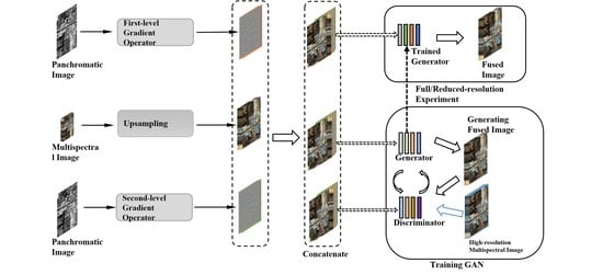
Therefore, to solve the problems of the PSGAN, this paper proposes a pansharpening GAN with multilevel structure enhancement and a multistream fusion architecture. The main contributions of this paper are as follows.

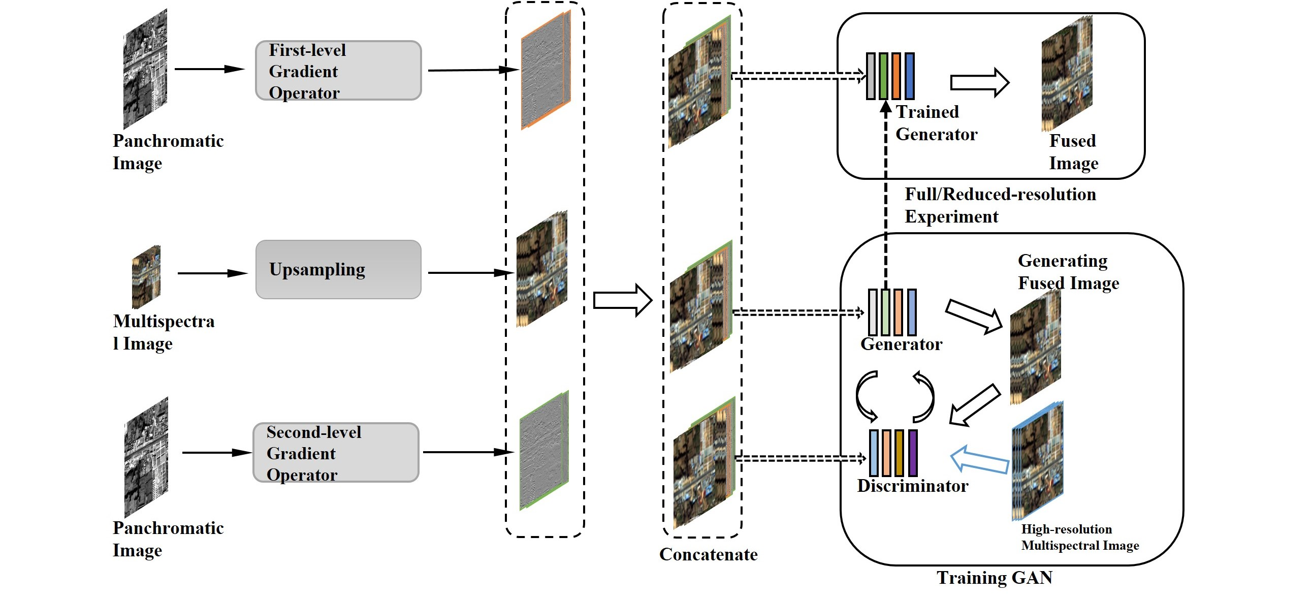
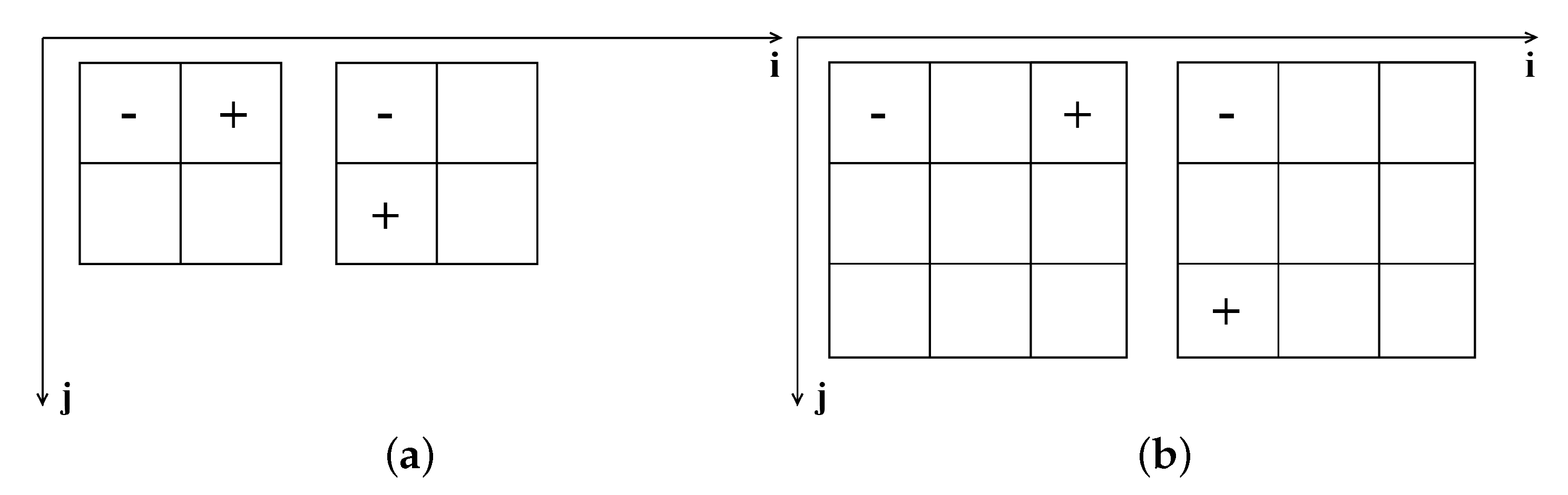
(1) We use multi-level differential operators to extract the spatial features of the panchromatic image, and fully integrate the spatial features of different levels with the spectral features. So that the spatial information of the fusion image can be fully expressed. Specifically, we used two types of gradient operators in the paper, the first-level gradient operator and the second-level gradient operator.

(2) In order to better combine the spatial information extracted by the multi-level gradient operator, we use the multi-stream fusion CNN architecture as the GAN generator. The multi-stream fusion architecture consists of three inputs and two sub-networks. Different types of structural information are input into specific subnets to better maintain structural and spectral information.

(3) We designed a comprehensive loss function. The loss function comprehensively considers the spectral loss, multi-level structure loss and adversarial loss. Among them, the multi-level structure loss combines two types of gradient operators to better give the optimization direction of network training, so that the extraction of structure information is more sufficient.

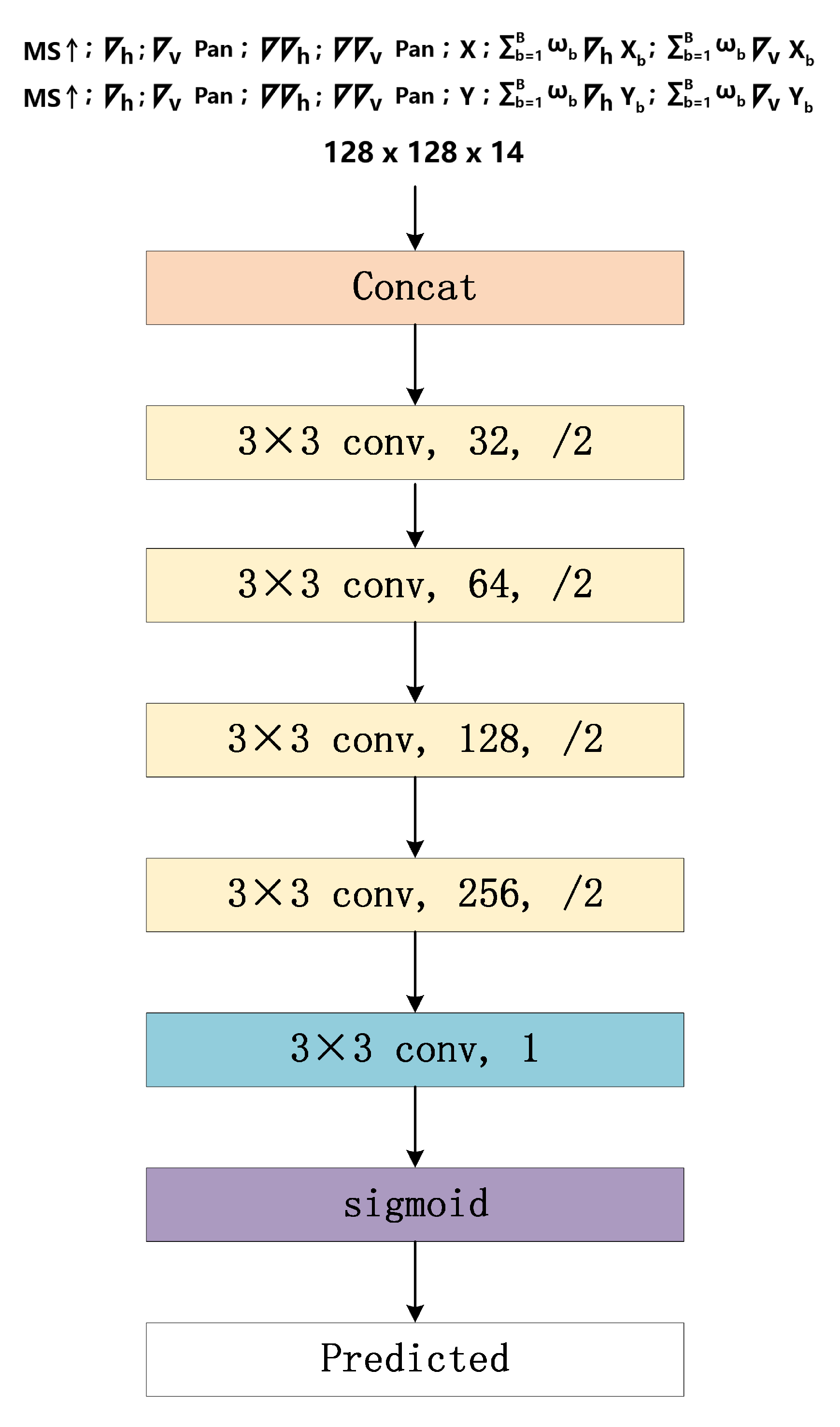
(4) To make it easier for the discriminator to distinguish real and fake images, we provide as much spectral and structural information as possible.

The remainder of the paper is organized as follows. Section 2 introduces the related work. Section 3 describes the method proposed in this paper. Section 4 presents the experiment and discussion. Section 5 is the conclusions.

2. Related Work

As pan-sharpening has attracted much attention, deep learning methods have been widely used in it. Researchers have proposed a lot of pan-sharpening methods based on deep learning according to different strategy modes, which have shown excellent nonlinear expression ability. Some methods choose simple shallow convolutional network as the architecture of training network, and extract the features from the input data using different techniques and strategies. For example, PCNN uses a simple three-layer convolutional network, and manually extracts important features such as the normalized water index (NDWI) as the input of the network [15]. Some methods choose to introduce excellent modules or architectures that are widely used in other fields of deep learning. For example, PANNET introduces residual network and uses high-pass filtering to extract the features of high-pass filtering domain from the input images, so that the network only needs to recover high-frequency information and can migrate between satellites with different numerical imaging ranges [17]. In [22], the author introduced Densely connected convolutional networks [23], which improved the ability to express spectral and spatial characteristics. In [24], the author proposed a multi-scale channel attention mechanism for panchromatic sharpening based on the channel attention mechanism originally applied to image classification work. This method considers the interdependence between channels and uses the attention mechanism to recalibrate, so as to perform feature representation more accurately. In both PSGAN and Pan-GAN [25], the author introduces generative confrontation network as the main architecture. PSGAN proposes to use dual-stream input to allow image feature-level fusion instead of pixel-level fusion. Pan-GAN adopts a method of establishing confrontational games between the generator and the spectral discriminator and the spatial discriminator, so as to retain the rich spectral information of the multi-spectral image and the spatial information of the panchromatic image. Some other methods use strategies to improve the loss function to optimize the training direction of the network. For example, in [26], the author proposed a perceptual loss function and further optimized the model based on advanced features in the near-infrared space. In general, the purpose of panchromatic sharpening is to obtain high-resolution multispectral images through fusion, and to preserve the spectral information of the multispectral images and the spatial information of the panchromatic images to the greatest extent. The methods mentioned above focus on the improvement of a certain aspect, or the simple application of a certain technology. These methods lack comprehensive leverage of image preprocessing, feature extraction, attention module, and loss function improvement. It is critical that how to use more than two technologies in one pansharpening method reasonably. This idea inspired our work.

3. Method

3.1. Pansharpening Based on a Variational Model and a GAN

The purpose of pansharpening is to fuse LRMS images and high-resolution PAN images. $P\in {\mathbb{R}}^{\mathrm{H}\times \mathrm{W}}$ represents the PAN image, $M=(M_1,M_2,\dots ,M_B)\in {\mathbb{R}}^{(\mathrm{H}/\mathrm{r})\times (\mathrm{W}/\mathrm{r})\times \mathrm{B}}$ represents the LRMS image, $M\uparrow =\left(M_1\uparrow ,M_2\uparrow ,\dots ,M_B\uparrow \right)\in {\mathbb{R}}^{\mathrm{H}\times \mathrm{W}\times \mathrm{B}}$ represents the LRMS image after upsampling, $X=(X_1,X_2,\dots ,X_B)\in {\mathbb{R}}^{\mathrm{H}\times \mathrm{W}\times \mathrm{B}}$ represents the image obtained by fusion, $Y=(Y_1,Y_2,\dots ,Y_B)\in {\mathbb{R}}^{\mathrm{H}\times \mathrm{W}\times \mathrm{B}}$ represents the real HRMS image, where $b=1,2,\dots ,B$ represents the number of channels of the image. r is 4 in this paper; that is, the resolution ratio of the PAN image to the MS image is 4:1.

Some pansharpening methods base on variational model have transformed the pansharpening process into an optimization problem solution process with reasonable hypotheses to achieve a good balance between spectral preservation and spatial restoration in fused images. The variational approaches usually assumes that the spatial information associated with each band of a fused image is consistent with that in a PAN image and the spectral information after the downsampling of the fused image is consistent with that in an LRMS image. For instance, Chen et al. [27] and Zeng et al. [12] use first-order finite difference operator to extract the sparse spatial structure information from the PAN image. Wang et al. [28] use second-order finite difference operator to extract spatial positions from the PAN image, such as corners, strongly textured regions, and edges. Inspired by these methods, we use two kinds of finite difference operators to extract the sparse spatial structure information from the PAN image. The first operator is the first-order finite difference operator. For the sake of simplicity, we call it as first-level gradient operator. The second operator is the second-level gradient operator. In fact, second-level gradient operator is also first-order finite difference operator. The main difference between the two operators is whether there is an interval of one pixel for the differential operation. The two operators are shown in Figure 1.

We use ∇ and $\nabla \nabla$ to represent the first-level gradient operator and second-level gradient operator, respectively. ${\nabla }_{h}P$ and ${\nabla }_{v}P$ represents the gradient information in two directions obtained by the first-level gradient operator. Among them, the subscript h represents the horizontal direction, and the subscript v represents the vertical direction. $\nabla {\nabla }_{h}P$ and $\nabla {\nabla }_{v}P$ represents the gradient information in two directions obtained by the second-level gradient operator. Through experiments, we found that the structural information fo the PAN image extracted by the second-level gradient operator is still rich, so we try to use the new structure to enhance the pansharpening performance. The two types of spatial structure inforamtion are shown in Figure 2.

The general form of the objective function in the fusion process is:

$$X=f\left(M,{\nabla }_{h}P,{\nabla }_{v}P,\nabla {\nabla }_{h}P,\nabla {\nabla }_{v}P;\Theta \right)$$

(1)

$f(•)$ can be regarded as a mapping function of X obtained from $(M,{\nabla }_{h}P,{\nabla }_{v}P,$$\nabla {\nabla }_{h}P,\nabla {\nabla }_{v}P)$, which means taking $M,{\nabla }_{h}P,{\nabla }_{v}P,\nabla {\nabla }_{h}P,\nabla {\nabla }_{v}P$ as the input; after a series of feature extractions, it is reformed into a full-sharpening model of HRMS image X. $\Theta$ represents the parameter set in the model. Therefore, we can reformulate pansharpening as an image generation problem that can be processed with a GAN. We first use a generator to map the joint distribution $p_d(M,{\nabla }_{h}P,{\nabla }_{v}P,\nabla {\nabla }_{h}P,\nabla {\nabla }_{v}P)$ to the target distribution $p_r\left(Y\right)$. Then, a corresponding discriminator is designed to estimate the probability that the sample comes from the training data and the generation model G so that the generator performs adversarial training to obtain a pansharpened image X that is closer to the target image Y. To make the presentation more convenient, we use ${▾}_h$ and ${▾}_v$ to represent all the gradient information in different directions (detailed expressions presented only when needed). Therefore, it can be expressed by the min-max problem of Equation (2):

$$\begin{array}{cc}\hfill \underset{{\Theta }_G}{min}\underset{{\Theta }_D}{max}& {\mathbb{E}}_{\left(M,{▾}_{h}P,{▾}_{v}P\right)\sim p_d\left(M,{▾}_{h}P,{▾}_{v}P\right),X\sim p_r\left(X\right)}\left[log{D}_{{\Theta }_D}(H,Z)\right]\hfill \\ \hfill & +{\mathbb{E}}_{\left(M,{▾}_{h}P,{▾}_{v}P\right)\sim p_d\left(M,{▾}_{h}P,{▾}_v\mathbf{P}\right)}\left[log\left(1-D_{{\Theta }_D}(H,F)\right)\right]\hfill \end{array}$$

(2)

where

$$H=[M\uparrow ;{▾}_{h}P;{▾}_{v}P]$$

$$Z=\left[Y;{▾}_h\sum _{b=1}^B{\omega }_b{Y}_b;{▾}_v\sum _{b=1}^B{\omega }_b{Y}_b\right]$$

$$\begin{array}{c}\hfill F=\left[G_{{\Theta }_G}\left(M,{▾}_{h}P,{▾}_{v}P\right);{▾}_h\sum _{b=1}^B{\omega }_b{G}_{{\Theta }_G}{\left(M,{▾}_{h}P,{▾}_{v}P\right)}_b;{▾}_v\sum _{b=1}^B{\omega }_b{G}_{{\Theta }_G}{\left(M,{▾}_{h}P,{▾}_{v}P\right)}_b\right]\end{array}$$

$[•;•]$ represents the concatenation operation, which is used to superimpose two or more tensors in the channel dimension. ${\omega }_b$ represents the relative weight coefficients of different satellite sensors obtained by the modulation transfer function (MTF) [10]. In addition, we improve the constraints of the generator based on the assumption of prior information and define the loss function of the generator as follows.

$$\mathcal{L}\left(G\right)={\mathcal{L}}_{\mathrm{adv}}+\lambda {\mathcal{L}}_{\mathrm{c}}$$

(3)

${\mathcal{L}}_{\mathrm{adv}}$ represents the adversarial loss between the generator G and the discriminator D. We define ${\mathcal{L}}_{\mathrm{adv}}$ as follows.

$${\mathcal{L}}_{\mathrm{adv}}=\frac{1}{N}\sum _{n=1}^N\left[-log{D}_{{\Theta }_D}(H,F)\right]$$

(4)

${\mathcal{L}}_{\mathrm{c}}$ is used to minimize the gap between the fused image and the real image, which is measured in terms of the spectra and structure.The reason for this design mainly comes from the inspiration of the variational model: First, the use of structural information; second, the use of its energy function to design the loss function. The first term is the spectral fidelity term. The second and third terms are the structure fidelity terms, which calculate the multilevel structure loss between the fused image and the PAN image. $\lambda$ is a hyperparameter used to balance ${\mathcal{L}}_{\mathrm{adv}}$, and ${\mathcal{L}}_{\mathrm{c}}$. ${\mu }_1$ and ${\mu }_2$ are used to weigh the ${\mathcal{L}}_{\mathrm{c}}$ weight of the information loss of two sparse structures. The details are as follows:

$$\begin{array}{c}\hfill {\mathcal{L}}_c=\frac{1}{N}\sum _{n=1}^N\left[{∥Y-G_{{\Theta }_G}\left(M,{▾}_{h}P,{▾}_{v}P\right)∥}_1+{\mu }_1{L}_{ss1}+{\mu }_2{L}_{ss2}\right]\end{array}$$

(5)

$$\begin{array}{c}\hfill L_{ss1}=\left({∥{\nabla }_{h}P-{\nabla }_h\sum _{b=1}^B{\omega }_b{G}_{{\Theta }_G}{\left(M,{\nabla }_{h}P,{\nabla }_{v}P\right)}_b∥}_1+{∥{\nabla }_{v}P-{\nabla }_v\sum _{b=1}^B{\omega }_b{G}_{{\Theta }_G}{\left(M,{\nabla }_{h}P,V_{v}P\right)}_b∥}_1\right)\end{array}$$

(6)

$$\begin{array}{c}\hfill L_{ss2}=\left({∥\nabla {\nabla }_{h}P-\nabla {\nabla }_h\sum _{b=1}^B{\omega }_b{G}_{{\Theta }_G}{\left(M,\nabla {\nabla }_{h}P,\nabla {\nabla }_{v}P\right)}_b∥}_1+{∥\nabla {\nabla }_{v}P-\nabla {\nabla }_v\sum _{b=1}^B{\omega }_b{G}_{{\Theta }_G}{\left(M,\nabla {\nabla }_{h}P,\nabla {\nabla }_{v}P\right)}_b∥}_1\right)\end{array}$$

(7)

where N represents the number of training samples. We derive the discriminator loss function based on the GAN principle:

$$\begin{array}{c}\hfill \mathcal{L}\left(D\right)=\frac{1}{N}\sum _{n=1}^N\left[log\left(1-D_{{\Theta }_D}(H,F)\right)\right]+\frac{1}{N}\sum _{n=1}^N\left[log{D}_{{\Theta }_D}(H,Z)\right]\end{array}$$

(8)

In summary, we proposed the use of multi-level gradient operators to extract different levels of spatial features, and designed the corresponding loss function. Among them, the loss function considers spectral loss and adversarial loss, and also combines two types of gradient operators to design a multi-level structure loss, which better gives the optimization direction of network training.

3.2. Multi-Stream Structure Generator and Discriminator

According to the overall design of the algorithm in Section 3.1, this paper proposes a generator combining a multistream structure, as shown in Figure 3. Different from traditional deep learning algorithms, the proposed method introduces the constraint of gradient information. That is, the first-level gradient operator and second-level gradient operator are used to extract the structure of the PAN image. We upsample the MS image to the resolution of the PAN image to obtain the MS↑ image. The MS↑ image, two gradient constraints and the original MS image are taken together as the input of the generator. Unlike the basic CNN, which directly stitches multiple images that need to be fused as input, we use subnetworks at the bottom of the network to extract hierarchical features for the MS↑ image and two types of structural information. The spectral and spatial information are extracted to obtain rich primary features. Then, the two types of structural information are combined with the spectral feature concatenation results after a series of feature extractions and supplementations. Finally, the joint features of the two results are mapped, and the required fusion image is reconstructed through transposed convolution decoding. A convolution kernel with a size of $2\times 2$, stride = 2, and padding = SAME is used to replace the downsampling operation, which better retains the perfect features. We used the leaky rectified linear unit (Leaky ReLU) activation function proposed in [29]. Inspired by U-Net [30], we adjust the network structure through skip connections. That is, the features of the lower layer are added to the higher layer by skipping the connection operation. The detailed architecture and convolution parameters are shown in Figure 3. The blue box represents the convolutional layer without downsampling. The yellow box represents the convolutional layer with downsampling. The red box represents the deconvolutional layer with upsampling.

In order to play zero sum game in the process of generating fused image, this paper designs a discriminator with neural network architecture. The discriminator is a simple five-layer convolutional neural network, which is used for distinguish whether each sample is a real HRMS image or a fused MS image. The detail architectures are shown in Figure 4. The yellow box represents the convolutional layer with downsampling. The blue box represents the convolutional layer without downsampling. Because of the particularity of sigmoid function in our network, we draw it after the final convolutional layer. The purple box represents the sigmoid function. The spectral information contains the upsampled MS image, the fused image X or the real image Y. The structural information contains the two-level horizontal and vertical gradient information of the PAN image, the fused image or the real image. For the Gaofen-2 dataset, the input data has 14 channels. We present the specific architecture in Figure 4. We use a simple CNN as the backbone structure of the discriminator. From the first layer to the fourth layer, a convolution kernel with a size of $3\times 3$, a step size of 2, is used for feature extraction. To reduce the effects of noise, all of our convolutional filters do not use padding operation. The last layer uses a sigmoid function to calculate the probability of the pixels in an image belong to a real image. The remaining convolutional layers are all activated by the Leaky ReLU activation function. In the implementation of the algorithm, we will input twice and pass the discriminator network twice. The main difference between the two inputs is the fused image X and the real image Y. We will calculate the log difference expectation for the two results. The final result is defined as the loss of the discriminator.

4. Experiments

4.1. Experimental Setup

We use the Gaofen-2 and WorldView-2 datasets to verify the effectiveness of the proposed method. The PAN images of the Gaofen-2 and WorldView-2 datasets have only one band, and the image resolutions are 0.81 m and 0.5 m, respectively. The MS image of the Gaofen-2 dataset has four bands, namely, red, green, blue, and near-infrared (NIR) bands, and the image resolution is 3.24 m. The MS image of the WorldView-2 dataset has 8 bands, namely, blue, green, red, coastal zone, yellow, red-edge and two sets of NIR spectra bands, and the image resolution is 1.8 m. Our experiment consists of three parts: Reduced resolution experiment, ablation experiment and full resolution experiment [31]. The comparative experiments select some algorithms introduced in the first section of this article. Specifically, for the multiresolution analysis ATWT algorithm, MTF-Generalized LP (MTF-GLP) [10], component replacement BDSD algorithm, and variational approach using spectral consistency and dynamic gradient sparsity (DGSF) [27]. Inspired by the deep learning-based methods and variational approaches, we have proposed a generative adversarial network with structural enhancement and spectral supplement for pan-sharpening (represented by “self-comparison” in our comparative experiment) [21]. For the parameters of each method, the settings recommended by the authors of the corresponding references are selected to make each method achieve the best results.

All the experiments of the deep learning-based methods in this paper involve training with an NVIDIA Tesla V100 SXM2 16 GB GPU and an Intel Xeon Gold 6148 at 2.40 GHz CPU. We use the pytorch framework to implement the deep learning-based methods and compare the computational times of each network. We use Adam [32] algorithm as the optimizer. For training our proposed network, the batch size is set to 16, the learning rate is set to 0.0002, the parameters of the Adam optimizer are set to 0.5 and 0.99, and a total of 20 epochs training are executed. According to the results of many experiments, the weight hyperparameters $\lambda$, ${\mu }_1$ and ${\mu }_2$ are set to 90, 80 and 40, respectively. The hyperparameters of other models are consistent with those in the original paper. The trained network can be reused for a long period of time from the same source of data for inference. The inference time required for our test set is usually within 1–2 s, which is at the same level as traditional component replacement algorithms. We list the time cost, parameter amount, and FLOPs for network training of reduced-resolution experiment on the WorldView-2 dataset, as shown in

Table 1. Comparison of the computational times of the compared network.

Method	Time (min)	Parameters	FLOPs
PCNN	$104\pm 10$	96.280 K	1.577 G
PANNET	$65\pm 10$	78.920 K	1.293 G
PSGAN	$169\pm 10$	2.441 M	33.787 G
Proposed	$214\pm 10$	6.702 M	25.884 G

.

4.2. Reduced-Resolution Experiment

We conducted a reduced-resolution experiment according to the Wald protocol [33], in which we used the original LRMS images as a reference. Before downsampling LRMS and PAN images, we smooth all original images using a filter that matches the MTF of the sensor [10,15,31]. Before smoothing, we trim the orignal LRMS images into patches with size of $128\times 128$, called as HRMS images, which should be used for reference, and the orignal PAN images into patches with size of $512\times 512$. Then we smooth them using Gaussian kernels with MTF, and downsample them to images with size of $32\times 32$ and size of $128\times 128$, respectively. Finally, we construct the corresponding data set for training and testing, in which one MS image with size of $32\times 32$, one PAN image with size of $32\times 32$ and one HRMS image with size of $128\times 128$ form a sample pair. We expect to get the fused images with size of $128\times 128$, which should be as identical as possible to the HRMS images. In our reduced-resolution experiment, we upsample the MS images in training set using the interpolation kernel proposed in [9] as input. In the samples obtained from the Gaofen-2 dataset, we selected 12,800 sample pairs as the training samples and 256 sample pairs as the testing samples. Since WorldView-2 has more data than Gaofen-2, we selected 12,800 sample pairs as training samples and 576 sample pairs as testing set. In terms of the results evaluation, we mainly use the spectral angle mapper (SAM) [31], relative dimensionless integrated global error in synthesis (ERGAS) [33], generalized image quality index (UIQI) to n-band extension ($Q_n$) [34], and the spatial correlation coefficient (SCC) [35] indexes for quality assessment. In the experimental results obtained in the testing set, we sampled ten small images of size $256\times 256$ and measured the quality indexes of these ten locations separately, calculated the average across all the results and compared the algorithms. For special objects, such as land, vegetation areas, buildings, and roads, in the fusion image, we conduct local-area experiments. Our process of conducting reduced-resolution experiment is shown in Figure 5.

It can be seen from Figure 5 that the setting conditions are slightly different based on the traditional method and the method based on deep learning. The traditional method is to use the image before cropping for fusion operation. There are two main reasons for this design.The first reason is that traditional methods, such as BDSD and DGSF, need to set hyperparameters to generate reasonable pan-sharpened images. However, taking the Gaofen-2 dataset as an example, our testing image size is $2048\times 2048$, which can be split into 256 patches of size $128\times 128$. It’s hard to adjust the model hyperparameters for each patch. The second reason is that the methods based on deep learning takes into account factors such as memory and time complexity, and usually cuts testing images into small image patches for processing. In addition, the operation of sharpening image patches and then splicing them into testing images has higher requirements for the pan-sharpening algorithm. Because the image patches does not have the gradient information around the edge, the fused image is prone to grid effect. Therefore, compared to sharpening image patches, the index of the deep learning methods will generally improve when directly sharpening testing image. Compared with sharpening testing image, the index of traditional learning methods are generally lower when directly sharpening image patches. Moreover, in our experiments, images generated by deep learning methods are generally better than those generated by traditional methods. Therefore, we only respectively guarantee the experimental conditions consistency of deep learning methods and traditional methods.

Figure 6 and Figure 7 show examples of the testing set fusion results of the Gaofen-2 and WorldView-2 datasets. To better judge the advantages and disadvantages of the fusion effect, we spliced the fused images with a size of $128\times 128$ into the size of the testing set. Then select an area with a resolution of $512\times 512$ for display, and zoom in on some details. It can be seen from the effect display diagram, especially Figure 6, that the four deep learning methods have better spectral and spatial structure information preservation than other methods. Traditional methods perform significantly poorly in areas such as vegetation and soil. The result of DGSF image fusion has obvious spots. ATWT and MTF-GLP have over-sharpening in some areas and distortion of texture details. The BDSD spectrum performs well, but there is obvious spatial detail distortion, showing a large area of blur. While methods based on deep learning outperform the traditional methods, the PCNN and PanNet still result in insufficient feature extraction and structure preservation. It can be observed from the effect display diagram, especially the Gaofen-2 display diagram, that the PCNN and PanNet perform poorly with respect to the image details. In the hyperspectral region, we can observe that the PSGAN removes some high-frequency details as noise, and there is excessive denoising. The proposed method can observe subtle differences in the enlarged detail area of the image. In general, the proposed algorithm achieves the best fusion effect in terms of the performance of the hyperspectral region and the reduction in the overall spectral and spatial information. The details are also shown in the residual diagrams shown in Figure 8 (Gaofen-2) and Figure 9 (WorldView-2). The residual image is obtained by subtracting the fusion result from the original LRMS image. In theory, the less texture the MS image contains, the better the fusion result is.

More detailed comparisons are shown in

Table 2. Indexes of fusion results for the reduced-resolution exmperiment on the Gaofen-2 dataset.

Method	SAM	ERGAS	${\mathit{Q}}_{\mathit{n}}$	SCC
ATWT	1.7525	2.1664	0.5545	0.5016
DGSF	2.0878	2.0419	0.5626	0.5308
MTF-GLP	1.8830	2.1133	0.6056	0.5330
BDSD	2.1964	1.8314	0.6620	0.6013
PCNN	1.3925	1.2026	0.8081	0.7897
PANNET	1.2200	1.0498	0.8406	0.8342
PSGAN	0.9567	0.8445	0.9098	0.9167
Self_comparison	0.9126	0.7946	0.9147	0.9231
Proposed	0.8671	0.7604	0.9294	0.9348
Reference	0	0	1	1

(Gaofen-2) and

Table 3. Indexes of the fusion results for the reduced-resolution exmperiment on the WorldView-2 dataset.

Method	SAM	ERGAS	${\mathit{Q}}_{\mathit{n}}$	SCC
ATWT	6.5497	3.0596	0.7602	0.7361
DGSF	6.9088	4.0796	0.6969	0.7237
MTF-GLP	6.5415	4.4157	0.7514	0.7360
BDSD	8.3306	3.4183	0.7365	0.7062
PCNN	5.4269	3.4702	0.8424	0.8929
PANNET	4.6383	2.9386	0.8538	0.9141
PSGAN	3.7764	2.4885	0.8780	0.9495
Self_comparison	3.6108	2.3521	0.8810	0.9523
Proposed	3.5641	2.3519	0.8868	0.9578
Reference	0	0	1	1

(WorldView-2). We mark the best indicator in bold in each subsequent table. From these tables, we can see that the traditional algorithms perform poorly in terms of the various quality indexes. The indexes of the neural network methods are significantly improved compared with those of the traditional algorithms. Considering the overall effectiveness of the image fusion step, the proposed method outperforms all the methods considered.

4.3. Ablation Experiment

For the ablation experiment, we extracted the main functional modules. We use only the first-level gradient operator to extract the structural information, and we remove the loss of the sparse structural information, extracted by the second-level gradient operator, in ${\mathcal{L}}_c$ (represented by “Only_spatial1” in the experimental part) to verify the function of the proposed new structural information extraction operator. In addition, we input two kinds of sparse structural information together with the spectral information into the generator with only one subnet to verify the function of the multistream structure compensation generator (represented by “One_subnet” in the experimental part).

We used Gaofen-2 and WorldView-2 datasets to conduct ablation experiments to prove the effectiveness of the module. Specifically, we use backbone to represent the basic network after removing the relevant modules. We use One_subnet to verify the role of the multi-stream structure generator, that is, to splice two types of structure information into a network with only one branch generator. We use Only_spatial1 to verify the effectiveness of the second-level gradient operator, that is, only use the first-level gradient operator to bring it into the multi-branch generator, and remove the constraint on the second-level gradient operator in the loss. In addition, we used the final network model with all modules as a comparison. The same data set as the simulation experiment was used for testing and verification. The experimental results show that the proposed final network method has achieved good results. In addition, when we control the use of related modules, we can see that some indicators show significant changes. The performance of specific indicators is shown in

Table 4. Index performance of ablation experiments on Gaofen-2 and WorldView-2 datasets.

Dataset	Backbone	Second-Level	Multi-Stream	Name	SAM	ERGAS	${\mathit{Q}}_{\mathit{n}}$	SCC
Gaofen-2	✔	✔		One_subnet	0.8813	0.7876	0.9189	0.9312
	✔		✔	Only_spatial1	0.9047	0.7802	0.9203	0.9306
	✔	✔	✔	Proposed	0.8671	0.7604	0.9294	0.9348
WorldView-2	✔	✔		One_subnet	3.6845	2.3758	0.8832	0.9543
	✔		✔	Only_spatial1	3.5872	2.3659	0.8841	0.9509
	✔	✔	✔	Proposed	3.5641	2.3519	0.8868	0.9578
				Reference	0	0	1	1

, and the performance of the effect diagram and residual diagram is shown in Figure 6, Figure 7, Figure 8 and Figure 9. The results in Table 4 show that the addition of the second-level gradient operator has a significant effect on the improvement of SCC indicators, especially the performance in the WorldView-2 data set. The multi-stream structure generator has an obvious effect on the overall effect, especially the improvement of the Qn index. In the details of the renderings and residual images, a conclusion consistent with the performance of the indicator can be observed.

4.4. Full-Resolution Experiment

For full-resolution experiments, we directly use the original LRMS images and PAN images as input, and bring them into the reduced-resolution model obtained by training. We still cut the MS image to a size of $32\times 32$ and the PAN image to a size of $128\times 128$. Different from the reduced-resolution experiment, the full-resolution experiment has no reference image to evaluate the advantages and disadvantages of the fusion effect. Therefore, we use the quality without reference (QNR) index [36] to evaluate the quality of the results. The QNR index includes an index $D_{\lambda }$ for evaluating the loss of spectral detail and an index $D_s$ for evaluating the loss of spatial detail.

Figure 10 shows the full-resolution image fusion result of the testing set obtained by WorldView-2. We still zoomed in on the $100\times 100$ area. Judging from the index results in

Table 5. Indexes of the fusion results for the full-resolution exmperiment on the WorldView-2 dataset.

Fusion Method	${\mathit{D}}_{\mathit{\lambda }}$	${\mathit{D}}_{\mathit{s}}$	QNR
ATWT	0.0728	0.1212	0.8148
DGSF	0.1029	0.1202	0.7893
MTF-GLP	0.0949	0.1438	0.7750
BDSD	0.0426	0.0637	0.8964
PCNN	0.0575	0.0655	0.8808
PANNET	0.0130	0.0312	0.9563
PSGAN	0.0142	0.0410	0.9453
Self_comparison	0.0134	0.0297	0.9573
Proposed	0.0127	0.0239	0.9638
Reference	0	0	1

, the neural network algorithm, especially the algorithm in this paper, is significantly better than other traditional algorithms. The algorithm in this paper uses the gradient operator to extract the structural information of the PAN image, which can better preserve the spatial structure information, and the corresponding spatial structure information loss index $D_s$ has been greatly improved. Moreover, because the method in this paper designs a reasonable loss function, the $D_{\lambda }$ spectral loss index has achieved better performance than other neural network algorithms. The overall indicators show that DGSF and MTF-GLP perform poorly in full-resolution experiments, whether it is the spectral loss indicator $D_{\lambda }$ or the spatial loss indicator $D_s$. ATWT spectral loss $D_{\lambda }$ performance is acceptable, but $D_s$ has not achieved very good performance. BDSD has achieved good results in traditional methods, even better than PCNN, but the overall performance is not as good as other neural network-based methods. A conclusion consistent with the index results can be observed at the details of the zoomed-in image. As can be seen from Figure 10, the fusion result of PanNet algorithm has achieved good results in terms of structural information and spectral information, but it is not good in terms of high-saturation color performance and structural details. While the PSGAN algorithm has achieved certain advantages in reduced-resolution experiments, some indicators, but for clearer full-resolution experiments, there is an over-sharpening phenomenon. Compared with other algorithms, the algorithm proposed in this paper can reduce the distortion of the spectrum to a greater extent, and it is more sufficient in the preservation of structural texture information.

4.5. Local Area Experiment

To prove the advantages of the proposed method, we perform more experiments on local areas in the WorldView-2 images. We take the land, vegetation areas, buildings, and roads in the fused image as the main objects and test the quality indexes for both the reduced-resolution and the full-resolution experiments. In these experiments, we select ten areas for each main object, which mainly contain the corresponding object, and then take the average of ten values as the final quality index value. We select three pansharpening methods based on deep neural network with excellent performance for the comparative experiments.

For the final experimental results, we selected a certain area of different objects for display, as shown in Figure 11, Figure 12, Figure 13, Figure 14, Figure 15, Figure 16, Figure 17 and Figure 18, and displayed the index test results in

Table 6. Land area in the reduced-resolution experiment.

Method	SAM	ERGAS	${\mathit{Q}}_{\mathit{n}}$	SCC
PCNN	2.1840	1.4834	0.6787	0.9313
PANNET	1.6128	1.1908	0.6794	0.9426
PSGAN	1.5504	1.0725	0.6662	0.9564
Proposed	1.4739	1.0197	0.6819	0.9610
Reference	0	0	1	1

,

Table 7. Land area in the full-resolution experiment.

Fusion Method	${\mathit{D}}_{\mathit{\lambda }}$	${\mathit{D}}_{\mathit{s}}$	QNR
PCNN	0.1531	0.1333	0.7358
PANNET	0.0693	0.0679	0.8694
PSGAN	0.0582	0.0860	0.8620
Proposed	0.0469	0.0399	0.9157
Reference	0	0	1

,

Table 8. Vegetation area in the reduced-resolution experiment.

Method	SAM	ERGAS	${\mathit{Q}}_{\mathit{n}}$	SCC
PCNN	4.9805	3.0891	0.8056	0.9106
PANNET	4.3985	2.6672	0.8192	0.9178
PSGAN	3.7217	2.2817	0.8497	0.9524
Proposed	3.5140	2.1630	0.8582	0.9603
Reference	0	0	1	1

,

Table 9. Vegetation area in the full-resolution experiment.

Fusion Method	${\mathit{D}}_{\mathit{\lambda }}$	${\mathit{D}}_{\mathit{s}}$	QNR
PCNN	0.0926	0.1294	0.7902
PANNET	0.0355	0.0688	0.8982
PSGAN	0.0349	0.0843	0.8838
Proposed	0.0227	0.0457	0.9327
Reference	0	0	1

,

Table 10. Buildings in the reduced-resolution experiment.

Method	SAM	ERGAS	${\mathit{Q}}_{\mathit{n}}$	SCC
PCNN	4.8930	3.0488	0.8580	0.9136
PANNET	4.2288	2.7276	0.8651	0.9281
PSGAN	3.4164	2.2940	0.8910	0.9586
Proposed	3.1903	2.1578	0.9012	0.9667
Reference	0	0	1	1

,

Table 11. Buildings in the full-resolution experiment.

Fusion Method	${\mathit{D}}_{\mathit{\lambda }}$	${\mathit{D}}_{\mathit{s}}$	QNR
PCNN	0.0419	0.0628	0.8984
PANNET	0.0205	0.0377	0.9428
PSGAN	0.0248	0.0496	0.9272
Proposed	0.0211	0.0270	0.9526
Reference	0	0	1

,

Table 12. Roads in the reduced-resolution experiment.

Method	SAM	ERGAS	${\mathit{Q}}_{\mathit{n}}$	SCC
PCNN	4.2356	2.8598	0.8164	0.8937
PANNET	3.6831	2.5245	0.8199	0.9083
PSGAN	3.0803	2.2228	0.8453	0.9377
Proposed	2.8836	2.0635	0.8577	0.9495
Reference	0	0	1	1

and

Table 13. Roads in the full-resolution experiment.

Fusion Method	${\mathit{D}}_{\mathit{\lambda }}$	${\mathit{D}}_{\mathit{s}}$	QNR
PCNN	0.1157	0.1483	0.7534
PANNET	0.0482	0.0896	0.8666
PSGAN	0.0536	0.1109	0.8415
Proposed	0.0517	0.0477	0.9030
Reference	0	0	1

. Among them, it can be seen that the resolution reduction experiment, the method proposed in this paper is better than the latest method in most quality indicators. In particular, the $Q_n$ index for overall image quality evaluation, and the SCC index for better characterization of spatial quality. This is due to the design of the multi-level gradient operator, loss function and generator we proposed. It is worth mentioning that in our proposed method, the improvement of vegetation and land is minimal for $Q_n$ index, vagetation and land. The road area improvement is the largest, which is about 1.5% higher than the other best quality indicators. In the resolution reduction image display image, the effect is limited by the naked eye, but it can still observe a subtle difference.For example, in the red part of the building area, it can be observed that the color saturation of PCNN and PANNET is insufficient, and the performance of the architectural details is poor. The color depth level of PSGAN in the vegetation area is not rich. For full-resolution experiments, we mainly focus on the results of index evaluation, because there is no image to refer to. The method we proposed performed best on the road area index, especially the QNR index rose by about 5%. In the performance of the full-resolution fusion image, PCNN performs poorly in areas with high color saturation, and there are traces of wire stitching in local areas. While PANNET is superior to PCNN in terms of spectral information, it is still insufficient in terms of preserving the details of buildings and road areas. PSGAN has achieved good visual effects in full-resolution experimental images, but the image processing is over-smooth. In addition, the retention of spectral information and the level of detail of structural information are not enough.

5. Conclusions

This paper proposes a panchromatic sharpening generation confrontation network with multi-level structure enhancement and multi-stream fusion architecture. Different from other neural network methods, we use multi-level gradient operators to obtain sparse structure information when processing panchromatic images. Moreover, we specifically designed a multi-stream fusion CNN architecture to build a GAN generator to better maintain structural information. In addition, we no longer use a single minimization strategy to minimize the gap between the fused image and the reference image. On this basis, we regard the loss of GAN and the information loss corresponding to the multi-level structure as the input of the optimization function. The appeal mentioned that our generator network does not use a simple shallow network, and the fusion result has more sufficient spectral information than the shallow neural network method. Due to our reasonable design of the generator and loss function for the multi-level gradient operator, we have better structural information retention for the corresponding deep neural network method. In the experimental part, we use the representative remote sensing image data sets Gaofen-2 and WorldView-2 to verify and analyze the proposed method. Experimental results show that our method is much better than the state-of-the-art methods, especially in the fields of construction and roads. The success of our method shows that extracting as much structural information of the panchromatic image as possible and using a multi-stream network structure can effectively improve the quality index. Unfortunately, there are multiple hyperparameter settings in the loss function design of our method, which brings complexity to the application in different fields. In the future, we will design more innovative network architectures and reduce the involvement of hyperparameters.

References

1. Loncan, L.; De Almeida, L.B.; Bioucas-Dias, J.M.; Briottet, X.; Chanussot, J.; Dobigeon, N.; Fabre, S.; Liao, W.; Licciardi, G.A.; Simoes, M.; et al. Hyperspectral pansharpening: A review. IEEE Geosci. Remote Sens. Mag. 2015, 3, 27–46. [Google Scholar] [CrossRef] [Green Version]
2. Gaetano, R.; Masi, G.; Poggi, G.; Verdoliva, L.; Scarpa, G. Marker-controlled watershed-based segmentation of multiresolution remote sensing images. IEEE Trans. Geosci. Remote Sens. 2014, 53, 2987–3004. [Google Scholar] [CrossRef]
3. Liu, P.; Xiao, L.; Zhang, J.; Naz, B. Spatial-Hessian-feature-guided variational model for pan-sharpening. IEEE Trans. Geosci. Remote Sens. 2015, 54, 2235–2253. [Google Scholar] [CrossRef]
4. Shettigara, V.K. A generalized component substitution technique for spatial enhancement of multispectral images using a higher resolution data set. Photogramm. Eng. Remote Sens. 1992, 58, 561–567. [Google Scholar]
5. Feng, J.; Zeren, L.; Xia, C.; Zhiliang, W. Remote sensing image fusion method based on PCA and NSCT transform. J. Graphics 2017, 38, 247–252. [Google Scholar]
6. Rahmani, S.; Strait, M.; Merkurjev, D.; Moeller, M.; Wittman, T. An adaptive IHS pan-sharpening method. IEEE Geosci. Remote Sens. Lett. 2010, 7, 746–750. [Google Scholar] [CrossRef] [Green Version]
7. Garzelli, A.; Nencini, F.; Capobianco, L. Optimal MMSE pan sharpening of very high resolution multispectral images. IEEE Trans. Geosci. Remote Sens. 2007, 46, 228–236. [Google Scholar] [CrossRef]
8. Shensa, M.J. The discrete wavelet transform: Wedding the a trous and Mallat algorithms. IEEE Trans. Signal Process. 1992, 40, 2464–2482. [Google Scholar] [CrossRef] [Green Version]
9. Aiazzi, B.; Alparone, L.; Baronti, S.; Garzelli, A. Context-driven fusion of high spatial and spectral resolution images based on oversampled multiresolution analysis. IEEE Trans. Geosci. Remote Sens. 2002, 40, 2300–2312. [Google Scholar] [CrossRef]
10. Aiazzi, B.; Alparone, L.; Baronti, S.; Garzelli, A.; Selva, M. MTF-tailored multiscale fusion of high-resolution MS and Pan imagery. Photogramm. Eng. Remote Sens. 2006, 72, 591–596. [Google Scholar] [CrossRef]
11. Zheng, X.H.Z.Q. A fusion method of satellite remote sensing image based on IHS transform and curvelet transform. J. South China Univ. Technol. 2016, 44, 58. [Google Scholar]
12. Zeng, D.; Hu, Y.; Huang, Y.; Xu, Z.; Ding, X. Pan-sharpening with structural consistency and 1/2 gradient prior. Remote Sens. Lett. 2016, 7, 1170–1179. [Google Scholar] [CrossRef]
13. Li, S.; Yang, B. A new pan-sharpening method using a compressed sensing technique. IEEE Trans. Geosci. Remote Sens. 2010, 49, 738–746. [Google Scholar] [CrossRef]
14. Liu, Y.; Chen, X.; Wang, Z.; Wang, Z.J.; Ward, R.K.; Wang, X. Deep learning for pixel-level image fusion: Recent advances and future prospects. Inf. Fusion 2018, 42, 158–173. [Google Scholar] [CrossRef]
15. Masi, G.; Cozzolino, D.; Verdoliva, L.; Scarpa, G. Pansharpening by convolutional neural networks. Remote Sens. 2016, 8, 594. [Google Scholar] [CrossRef] [Green Version]
16. Dong, C.; Loy, C.C.; He, K.; Tang, X. Image super-resolution using deep convolutional networks. IEEE Trans. Pattern Anal. Mach. Intell. 2015, 38, 295–307. [Google Scholar] [CrossRef] [PubMed] [Green Version]
17. Yang, J.; Fu, X.; Hu, Y.; Huang, Y.; Ding, X.; Paisley, J. PanNet: A deep network architecture for pan-sharpening. In Proceedings of the IEEE International Conference on Computer Vision, Venice, Italy, 22–29 October 2017; pp. 5449–5457. [Google Scholar]
18. He, K.; Zhang, X.; Ren, S.; Sun, J. Deep residual learning for image recognition. In Proceedings of the IEEE Conference on Computer Vision and Pattern Recognition, Las Vegas, NV, USA, 27–30 June 2016; pp. 770–778. [Google Scholar]
19. Liu, X.; Wang, Y.; Liu, Q. PSGAN: A generative adversarial network for remote sensing image pan-sharpening. In Proceedings of the 2018 25th IEEE International Conference on Image Processing (ICIP), Athens, Greece, 7–10 October 2018; pp. 873–877. [Google Scholar]
20. Goodfellow, I.; Pouget-Abadie, J.; Mirza, M.; Xu, B.; Warde-Farley, D.; Ozair, S.; Courville, A.; Bengio, Y. Generative adversarial nets. arXiv 2014, arXiv:1406.2661. [Google Scholar]
21. Zhang, L.; Li, W.; Zhang, C.; Lei, D. A generative adversarial network with structural enhancement and spectral supplement for pan-sharpening. Neural Comput. Appl. 2020, 32, 18347–18359. [Google Scholar] [CrossRef]
22. Xiang, Z.; Xiao, L.; Liu, P.; Zhang, Y. A Multi-Scale Densely Deep Learning Method for Pansharpening. In Proceedings of the IGARSS 2019—2019 IEEE International Geoscience and Remote Sensing Symposium, Yokohama, Japan, 28 July–2 August 2019; pp. 2786–2789. [Google Scholar]
23. Huang, G.; Liu, Z.; Van Der Maaten, L.; Weinberger, K.Q. Densely connected convolutional networks. In Proceedings of the IEEE Conference on Computer Vision and Pattern Recognition, Honolulu, HI, USA, 21–26 July 2017; pp. 4700–4708. [Google Scholar]
24. Li, X.; Xu, F.; Lyu, X.; Tong, Y.; Chen, Z.; Li, S.; Liu, D. A remote-sensing image pan-sharpening method based on multi-scale channel attention residual network. IEEE Access 2020, 8, 27163–27177. [Google Scholar] [CrossRef]
25. Ma, J.; Yu, W.; Chen, C.; Liang, P.; Guo, X.; Jiang, J. Pan-GAN: An unsupervised pan-sharpening method for remote sensing image fusion. Inf. Fusion 2020, 62, 110–120. [Google Scholar] [CrossRef]
26. Wang, J.; Shao, Z.; Huang, X.; Lu, T.; Zhang, R.; Ma, J. Pan-sharpening via High-pass Modification Convolutional Neural Network. arXiv 2021, arXiv:2105.11576. [Google Scholar]
27. Chen, C.; Li, Y.; Liu, W.; Huang, J. Image fusion with local spectral consistency and dynamic gradient sparsity. In Proceedings of the IEEE Conference on Computer Vision and Pattern Recognition, Columbus, OH, USA, 23–28 June 2014; pp. 2760–2765. [Google Scholar]
28. Wang, T.; Fang, F.; Li, F.; Zhang, G. High-Quality Bayesian Pansharpening. IEEE Trans. Image Process. 2019, 28, 227–239. [Google Scholar] [CrossRef]
29. Maas, A.L.; Hannun, A.Y.; Ng, A.Y. Rectifier nonlinearities improve neural network acoustic models. Proc. Icml 2013, 30, 3. [Google Scholar]
30. Ronneberger, O.; Fischer, P.; Brox, T. U-net: Convolutional networks for biomedical image segmentation. In Proceedings of the International Conference on Medical Image Computing and Computer-Assisted Intervention, Munich, Germany, 5–9 October 2015; Springer: Cham, Switzerland, 2015; pp. 234–241. [Google Scholar]
31. Vivone, G.; Alparone, L.; Chanussot, J.; Dalla Mura, M.; Garzelli, A.; Licciardi, G.A.; Restaino, R.; Wald, L. A critical comparison among pansharpening algorithms. IEEE Trans. Geosci. Remote Sens. 2014, 53, 2565–2586. [Google Scholar] [CrossRef]
32. Kingma, D.P.; Ba, J. Adam: A method for stochastic optimization. arXiv 2014, arXiv:1412.6980. [Google Scholar]
33. Wald, L. Data Fusion: Definitions and Architectures—Fusion of Images of Different Spatial Resolutions; Les Presses des Mines: Paris, France, 2002. [Google Scholar]
34. Garzelli, A.; Nencini, F. Hypercomplex quality assessment of multi/hyperspectral images. IEEE Geosci. Remote Sens. Lett. 2009, 6, 662–665. [Google Scholar] [CrossRef]
35. Zhou, J.; Civco, D.; Silander, J. A wavelet transform method to merge Landsat TM and SPOT panchromatic data. Int. J. Remote Sens. 1998, 19, 743–757. [Google Scholar] [CrossRef]
36. Alparone, L.; Aiazzi, B.; Baronti, S.; Garzelli, A.; Nencini, F.; Selva, M. Multispectral and panchromatic data fusion assessment without reference. Photogramm. Eng. Remote Sens. 2008, 74, 193–200. [Google Scholar] [CrossRef] [Green Version]
Figure 1. Two kinds of finite difference operators. (a) first-level gradient operator, (b) second-level gradient operator.
Remotesensing 13 02423 g001
Figure 2. Comparison of structural information. (a) PAN image, (b) horizontal structural information with first-level gradient operator, (c) vertical structural information with first-level gradient operator, (d) horizontal structural information with second-level gradient operator, (e) vertical structural information with second-level gradient operator.
Remotesensing 13 02423 g002
Figure 3. Detailed architectures of the Generator.
Remotesensing 13 02423 g003
Figure 4. Detailed architectures of the Discriminator.
Remotesensing 13 02423 g004
Figure 5. Flow chart of reduced-resolution exmperiment.
Remotesensing 13 02423 g005
Figure 6. Fusion results from the reduced-resolution experiment on the Gaofen-2 dataset.
Remotesensing 13 02423 g006
Figure 7. Fusion results from the reduced-resolution experiment on the WorldView-2 dataset.
Remotesensing 13 02423 g007
Figure 8. Residual images from the reduced-resolution experiment on the Gaofen-2 dataset.
Remotesensing 13 02423 g008
Figure 9. Residual images from the reduced-resolution experiment on the WorldView-2 dataset.
Remotesensing 13 02423 g009
Figure 10. Fusion results from the full-resolution experiment on the WorldView-2 dataset.
Remotesensing 13 02423 g010
Figure 11. The performance of the land area in the reduced-resolution experiment.
Remotesensing 13 02423 g011
Figure 12. The performance of the land area in the full-resolution experiment.
Remotesensing 13 02423 g012
Figure 13. The performance of the vegetation area in the reduced-resolution experiment.
Remotesensing 13 02423 g013
Figure 14. The performance of the vegetation area in the full-resolution experiment.
Remotesensing 13 02423 g014
Figure 15. The performance of the building area in the reduced-resolution experiment.
Remotesensing 13 02423 g015
Figure 16. The performance of the building area in the full-resolution experiment.
Remotesensing 13 02423 g016
Figure 17. The performance of the road area in the reduced-resolution experiment.
Remotesensing 13 02423 g017
Figure 18. The performance of the road area in the full-resolution experiment.
Remotesensing 13 02423 g018