A Nowcast/Forecast System for Japan’s Coasts Using Daily Assimilation of Remote Sensing and In Situ Data

Abstract

We have developed an ocean state nowcast/forecast system (JCOPE-T DA) that targets the coastal waters around Japan and assimilates daily remote sensing and in situ data. The ocean model component is developed based on the Princeton Ocean Model with a generalized sigma coordinate and calculates oceanic conditions with a 1/36-degree (2–3 km) resolution and an hourly result output interval. To effectively represent oceanic phenomena with a spatial scale smaller than 100 km, we adopted a data assimilation scheme that explicitly separates larger and smaller horizontal scales from satellite sea surface temperature data. Our model is updated daily through data assimilation using the latest available remote-sensing data. Here we validate the data assimilation products of JCOPE-T DA using various kinds of in situ observational data. This validation proves that the JCOPE-T DA model output outperforms those of a previous version of JCOPE-T, which is based on nudging the values of temperature and salinity toward those provided by a different coarse grid data-assimilated model JCOPE2M. Parameter sensitivity experiments show that the selection of horizontal scale separation parameters considerably affects the representation of sea surface temperature. Additional experiments demonstrate that the assimilation of daily-updated satellite sea surface temperature data actually improves the model’s efficiency in representing typhoon-induced disturbances of sea surface temperature on a time scale of a few days. Assimilation of additional in situ data, such as temperature/salinity/ocean current information, further improves the model’s ability to represent the ocean currents near the coast accurately.

1. Introduction

Ocean state forecast (OSF), particularly targeting ocean mesoscale phenomena, has been mainly using satellite sea surface height anomaly (SSHA) data for capturing the target phenomena through data assimilation (DA) since pioneering works in the 1990s (e.g., [1]). Other typical satellite remote-sensing data of ocean, sea surface temperature (SST), have also been used by OSF for correcting the water mass property mainly above the surface mixed layer [2]. Combined assimilation of remote sensing and in situ temperature/salinity profiles (TS) data has been developed since the appearance of ARGO floats [3]. Presently, basin-scale operational OSF systems using various kinds of observation data have been established [4]. The targeted spatiotemporal scales of the basin-scale operational OSF systems are O (100 km) and O (10 day) [3,4]. The satellite SSH measurements with a minimum sampling scale of 100 km and a major sampling period of 10 days fulfill the requirements for DA in a basin-scale operational OSF system.

Recently some operational OSF systems have been updated to target sub-mesoscale phenomena with spatially smaller (<100 km) and temporally shorter (<10 day) scales by using higher-resolution downscaled ocean models (e.g., [5]). Advanced DA schemes, including four-dimensional variational methods (e.g., [6]) and an ensemble Kalman Filter (e.g., [7]), have been developed to effectively extract the observational information required to downscale from satellite SSHA and SST data. In addition, concurrent simulation of geostrophic and tidal currents using higher-resolution ocean general circulation models (OGCMs) has been developed [8,9].

The Japan Coastal Ocean Predictability Experiment (JCOPE), promoted by Japan Agency for Marine–Earth Science and Technology (JAMSTEC), has aimed at operational modeling of the mesoscale phenomena in the Northwest Pacific Ocean. The DA systems have been gradually updated: optimum interpolation (JCOPE1 [10]), three-dimensional variational (3dVar) (JCOPE2 [11]), and multi-scale 3dVar (ms3dVar) (JCOPE2M [12]). Recently, a downscaled OSF system targeting smaller spatial and shorter temporal scale phenomena (JCOPE-T DA) has been developed through collaboration between a satellite remote-sensing research group of the Japan Aerospace Exploration Agency (JAXA) and the JCOPE group. The JCOPE-T DA system provides oceanic state variables (sea level, temperature, salinity, and ocean current velocities) with an hourly interval in a region of 17°–50° N and 117°–150° E (Figure 1) with a horizontal resolution of 1/36 degree and 46 active vertical levels for the period from 1 January 2018 to the present. The major ocean currents around Japan’s coasts (Figure 1) are targeted by JCOPE-T DA. The resulting new products are utilized for scientific/engineering studies and also are available for industry use by the shipping, fishing, ocean renewable energy development, and undersea resources industries.

The major changes to the previous version of the OSF system (JCOPE2M) include:

(1)

The horizontal resolution change from 1/12 to 1/36 degree;

(2)

The oceanic state DA update interval change from 4 days to 1 day; and,

(3)

The use of a more accurate representation of the tidal currents (a critical step to correctly estimate a realistic initial condition for a model that can output daily forecasts).

There are two ways of assimilating the observed data into the downscaled OSF systems: indirect and direct DA approaches. The indirect approach is based on using other data-assimilative model outputs as references. The previous version of JCOPE-T took the indirect DA approach with relaxation (nudging) to the model temperature and salinity toward the JCOPE2M temperature and salinity, respectively [9]. The indirect approach saves the computational costs incurred by the DA procedures, although the performances of the resulting DA outputs depend on the outputs of the reference models. The direct DA approach simply applies the usual DA procedures to the ocean model components and requires some additional computational resources for the DA operation.

This study compares the model output of the indirect DA approach used by the previous version of JCOPE-T, to the model output of JCOPE-T DA using the direct DA approach. Since applying the direct approach with the advanced DA methods to the high-resolution downscaled models requires huge amounts of computational resources, the DA method with a relatively moderate computational cost (ms3dVar) is adopted for JCOPE-T DA.

JCOPE-T DA has been designed to utilize satellite SST products that are developed and distributed by JAXA for contributing to the Group for High-Resolution Sea Surface Temperature (GHRSST) [13]. Multiple daily composite data from the GHRSST products have been assimilated into the model. In this study, we explore the impacts of assimilating the satellite-based daily SST data into JCOPE-T DA by conducting a sensitivity experiment that assimilates another SST data set that has been temporally smoothed with a relatively coarse horizontal resolution.

Although the direct DA approach that uses the assimilation of the satellite-based SST adopted for JCOPE-T DA effectively works, it requires some parameters to be further fine-tuned. This study shows that the scale separation parameter in the ms3dVar scheme is the parameter that can critically affect the representation of the model SST. Other parameters examined in this study show no significant sensitivity.

In the present study, we evaluate the quality of the DA products by comparing them with various types of observational data, such as the satellite-based SST, in situ TS data, in situ ocean current data, sea level anomaly at tide gauge sites, and Kuroshio path position south of Japan reported by the Japan Coast Guard. Since JCOPE-T DA is mainly based on the assimilation of remote-sensing data (SSHA and SST), with the exception of the satellite-based SST, the observational data needed for validation are basically independent of the JCOPE-T DA products.

We further investigate the impacts of assimilating in situ TS and ocean current data into JCOPE-T DA to demonstrate the potential roles of using real-time in situ data for these two parameters for assimilation. In Japan, the in situ TS and ocean current data information obtained mainly by public operational agencies is usually transferred to the domestic/international data archives. The data transfer timing is not performed in real-time, and sometimes the actual measurements are delayed by nearly one month. We also discuss the benefits and feasibility of daily-basis assimilations for the in situ data as well as the remote-sensing data.

This paper is organized as follows. Section 2 describes the ocean model JCOPE-T, the DA algorithm, preprocessing of JAXA’s multiple SST products, and the observation data used for the validation. Contents of the performed experiments are also described in Section 2. Results of the sensitivity experiments are reported in Section 3 and discussed in Section 4. Section 5 concludes the present study. The Appendix A provides details of the DA algorithm and the DA parameters examined in the sensitivity experiments.

2. Methods and Data

2.1. A Regional Tide-Resolving Ocean Model JCOPE-T

A tide-resolving ocean general circulation model JCOPE-T [9] was used as a model component of the system. The ocean circulation model was based on the Princeton Ocean Model with a generalized coordinate of sigma [14] and completely rewritten for parallel computation using the Message Passing Interface. The model covered a horizontal range of 17°–50° N and 117°–150° E (Figure 1) with a resolution of 1/36 degree and 46 active vertical layers. The mixed layer physics was represented by Mellor–Yamada–Nakanishi–Niino–Furuichi‘s turbulence parameterization [15,16].

The atmospheric forcing data, including wind stress and latent/sensible heat fluxes, were estimated at sea surface with the use of the bulk formulas proposed by [17]. The short-wave radiation at the sea surface included the daily cycle, and it was estimated by analytical formulas that depended on the calendar time, geographical position, cloudiness [18,19], and an albedo model of [20]. The short-wave radiation penetrated the subsurface layer with a 23 m depth scale, assuming Jerlov’s water type I [21], and the part penetrating below the bottom was ignored. The longwave radiation was estimated following [22]. The atmospheric data required for the calculation of the bulk formulas were obtained from the global forecast system (GFS) of National Centers for Environmental Prediction (NCEP) and were hourly data that included analyses and hourly forecasts of up to 5 days followed by 3 h forecasts for 16 days in the future. NCEP updates meteorological forecasts every 6 h. Meteorological analyses and up to 6 h forecasts from each NCEP GFS bulletin are locally archived for utilization in the delayed mode re-integration of the JCOPE-T-DA system. The freshwater flux was applied at the sea surface to represent the effects of precipitation and evaporation. The freshwater discharge from the land was represented as water volume fluxes at river mouth grids with monthly mean climatological discharge volumes [9]. The open boundary condition was provided from daily mean velocities, temperature, salinity, and sea level data derived from the data-assimilated JCOPE2M ocean model, which covers the Northwest Pacific (10.5° N–62° N and 108° E–180° E) with a horizontal 1/12-degree resolution [12].

To represent the tidal current effects, the model put volume fluxes and sea level anomalies of 11 tidal constituents: Q1, O1, P1, K1, N2, M2, S2, K2, M4, MS4, MN4, at lateral boundaries. Information on the tidal components was provided by a 1/12-degree version model of Oregon State University Tidal Inversion Software (OTIS) [23]. In addition, the surface pressure gradient included the equilibrium gradient induced by 25 potential tidal constituents: Q1, O1, M1, P1, K1, J1, OO1, 2N2, MU2, N2, NU2, M2, L2, T2, S2, K2, M4, MS4, MN4, MM, MF, SSA, SA, MTM, MSQM. All other details of the model algorithm and validation of the simulated tidal phenomena are described in our previous paper [9].

2.2. Daily-Basis DA and Operational Forecast

The most significant update to the previous version of JCOPE-T [9] is a DA algorithm directly assimilating the observation data including satellite SSHA, satellite SST, and in situ TS profiles daily, while the previous version indirectly represents the DA effects by nudging temperature and salinity variables toward temperature and salinity data, respectively, provided by the other data-assimilative model JCOPE2M [12]. The ms3dVar scheme was applied to effectively represent the fine structures of TS associated with the oceanic variability at a relatively moderated computational cost for the daily operation [12] as compared to the other advanced DA methods, e.g., ensemble Kalman Filter [7]. The TS data produced by ms3dVar were inserted into the model through the Incremental Analysis Update algorithm [24]. Details of the DA algorithm are described in the Appendix A.

The JCOPE-T DA system has two modes of forecast operation: the daily mode and the delayed mode. The daily operation performs the DA run starting from 10 days before the current date and the succeeding 9-day lead forecast run. Once a week, the delayed mode operation performs the DA run starting from 1 month before the current date and the succeeding 3-week forecast run.

The delayed mode operation was required for assimilating the in situ TS data accumulated from the Global Temperature Salinity Profile Program (GTSPP) archive [25] because the GTSPP archive usually does not allow for the real-time acquisition of the in situ TS data owing to the inclusion of manual operations for the data input, and accumulation of the data is basically delayed compared to the timing of actual measurements. In contrast, satellite remote sensing data are automatically accumulated in the data archives that are automatically accessible through internet communication. The daily-mode operation mainly assimilates the remote-sensing data.

2.3. Multiple Satellite SST Products with Bias Correction

The model assimilated two types of satellite SST products: microwave and infrared SSTs. Microwave SST has the cloud-penetrating capability but coarse spatial resolution around 30–50 km, while infrared SST has a fine spatial resolution around 0.25–2 km but cannot measure SST under clouds.

The model assimilated three microwave SST products retrieved by the Advanced Microwave Scanning Radiometer 2 (AMSR2) onboard the Global Change Observation Mission-Water (GCOM-W) satellite, Global Precipitation Measurement (GPM) Microwave Imager (GMI) onboard the GPM Core Observatory, WindSat on board the Coriolis satellite, and three infrared SST products: Advanced Himawari Imager (AHI) onboard the Geostationary Meteorological Satellite “Himawari-8”, Second-Generation Global Imager (SGLI) onboard the Global Change observation Mission-Climate (GCOM-C) satellite, and Visible Infrared Imaging Radiometer Suite (VIIRS) onboard the Suomi National Polar-orbiting Partnership (Suomi NPP) satellite. All microwave SST products based on the algorithm by [26] and infrared SST products based on the algorithm by [27,28] are developed and distributed by JAXA.

We validated the satellite-based SSTs using quality-controlled in situ SSTs provided by the in situ SST Quality Monitor (iQuam) [29] version 2.0 of the National Oceanic and Atmospheric Administration (NOAA). The validation result showed that the mean difference (bias) between AMSR2 and iQuam SSTs was relatively lower than those between the other products and iQuam SST. Furthermore, the seasonal dependence of AMSR2 bias was insignificant compared with those of the other products’ biases. Thus, we decided to use AMSR2 SST data as reference data for correcting the bias of the other products.

First, each SST product was gridded onto a 1/10-degree grid and converted to daily mean SST by making a composite of all data obtained within a day. Next, an additional correction term (ACT) of each product was calculated as follows:

$$\mathrm{ACT}(\mathrm{product})=\langle \overline{\mathrm{SST}(\mathrm{AMSR}2)-\mathrm{SST}(\mathrm{product})}\rangle$$

(1)

where overbar and angle bracket denote temporal and spatial running mean operations, respectively. Then, the corrected SST was calculated as,

$${\mathrm{SST}}_{\mathrm{c}}(\mathrm{product})=\mathrm{SST}(\mathrm{product})+\mathrm{ACT}(\mathrm{product})$$

(2)

The time scale of running means was determined as 7 days because we found that the temporal changes in the biases were considerably affected by weather disturbances with an approximate weekly time scale around Japan. Spatial smoothing was applied to ACTs for the infrared SST products with higher horizontal resolutions than the microwave AMSR2 product used as a reference of the bias correction. The spatial scales for running mean were determined as 1.2, 0.6, 1.0 degrees for the AHI, SGLI, VIIRS products, respectively.

A mean satellite SST product was further calculated as,

$${\mathrm{SST}}_{\mathrm{m}}=\{\begin{array}{cc}\mathrm{missing}\mathrm{value}& ({\displaystyle \sum _{\mathrm{product}}an(\mathrm{product},x,y)}=0)\\ \frac{1}{{\displaystyle \sum _{\mathrm{product}}an(\mathrm{product},x,y)}}{\displaystyle \sum _{\mathrm{produc}t}\mathrm{an}(\mathrm{product},\mathrm{x},\mathrm{y})·\mathrm{SST}\left(\mathrm{product}\right)}& ({\displaystyle \sum _{\mathrm{produc}t}an(\mathrm{product},x,y)}>0)\end{array}$$

(3)

only if a product is available at position (x,y), $an(\mathrm{product},\mathrm{x},\mathrm{y})=1$ (if missing, $an(\mathrm{product},\mathrm{x},\mathrm{y})=0$). To use the information of the fine-scale structures captured by the infrared SST products: in particular, SGLI and AHI, we produced the merged satellite SST product (${\mathrm{SST}}_{\mathrm{o}}$) as follows:

$${\mathrm{SST}}_{\mathrm{o}}:{\mathrm{SST}}_{\mathrm{c}}(SGLI)\to {\mathrm{SST}}_{\mathrm{c}}(AHI)\to {\mathrm{SST}}_{\mathrm{m}}$$

(4)

where a right arrow denotes overwriting of the target product on the grid. Figure 2 shows daily snapshots at the beginning of July (Figure 2a) and the end of August (Figure 2b) 2020. Although a composite of multiple model outputs can effectively reduce the data gap areas caused by cloud contamination, the data gaps do not disappear completely. Figure 2 shows the snapshots of ${\mathrm{SST}}_{\mathrm{o}}$ with the widest (Figure 2a) and second widest (Figure 2b) data gaps during the targeted two-month period. Both images depict the data gaps caused by seasonal events, such as a Baiu front around the East China Sea and south of Japan (Figure 2a) and a typhoon (Figure 2b).

2.4. In Situ Observation Data Used for Validation and Additional Assimilation

To examine the actual skill of the DA products in the daily-mode operation, we excluded the in situ TS data from the assimilation in most of the experiments except in some cases as described later. We thus validate the model products by comparing them with the independent in situ TS data.

For independent validation, we also used sea level data measured at tide gauge stations in the southern coasts of Japan (Figure 3) and acoustic doppler current profiler (ADCP) data obtained around Tosa Bay (see Figure 1 for the location). Barometric [30] and tidal [31] variations were subtracted from both observation and model sea level data to extract the information about the ocean current variations from the tide gauge data.

2.5. A Reference Case and Sensitivity Experiments

We analyzed the DA products created by the repeated step 1 and step 2 operations (Appendix A). Analysis of the forecast model was out of the scope of this study. Starting from the same initial conditions created by the JCOPE-T DA operational system with the default parameters, all DA experiments of JCOPE-T DA were conducted for a two-month period from 1 July to 31 August 2020. Products of the previous version of JCOPE-T based on the indirect DA approach, “NUDGI”, for the same period were used for comparison to the JCOPE-T DA products using the direct DA approach. Both of the model runs were initialized on 2 September 2019 with TS and horizontal velocity variables interpolated from those of the coarse grid JCOPE2M model.

We performed three categories of sensitivity experiments by changing parameters and assimilation data used in a base “BASEX” case, which was designed for simulating a situation in the daily-mode operations.

Table 1. Brief descriptions of all experiments.

Cases	Brief Description
	Category 0
NUDGI	Nudging to JCOPE2M TS data
BASEX	A base case, assimilating the merged satellite SST (${\mathrm{SST}}_{\mathrm{o}}$)
	Category 1
MGSST	Assimilating MGDSST instead of ${\mathrm{SST}}_{\mathrm{o}}$
EXLMS	Assimilating ${\mathrm{SST}}_{\mathrm{o}2}$ instead of ${\mathrm{SST}}_{\mathrm{o}}$
	Category 2
SSTSL	Increase the separation scale from 50 km to 150 km
SSTER	Decrease the normalized SST error from 1.0 to 0.5
IAUSM	Increase the IAU smoothing scale from 9 km to 27 km
200KM	Increase the 3dVar covariance scale from 100 km to 200 km south of Japan
SUMM3	SSTSL + SSTER + IAUSM
TSEOF	Using the different statics in MWR and decreasing SSH error from 0.1 m to 0.07 m in MWR and JSS + SUMM3
	Category 3
INSTS	Assimilating the in situ TS data into SUMM3
INTS2	Assimilating the in situ TS data into TSEOF
LOCVL	Assimilating the local ocean current data into INSTS

provides a list of the results for all cases with brief descriptions for each. Parameters used in the BASEX case and other cases are described in

Table A1. Parameters used in the sensitivity experiments.

	Sc (km)	SL (km)	Siau (km)	$\mathit{T}\mathit{e}\mathit{r}{\mathit{r}}_{\mathit{L}}(\mathit{n},0)$	EOF in 39.5N–45N and 140E–150E
BASEX MGSST EXLMS	50	100	9	$\sqrt{1-\sigma }{T}_{std}^o(n,0)$	EOF-A
SSTSL	150	100	9	$\sqrt{1-\sigma }{T}_{std}^o(n,0)$	EOF-A
SSTER	50	100	9	$0.5\sqrt{1-\sigma }{T}_{std}^o(n,0)$	EOF-A
IAUSM	50	100	27	$\sqrt{1-\sigma }{T}_{std}^o(n,0)$	EOF-A
200KM	50	200	9	$\sqrt{1-\sigma }{T}_{std}^o(n,0)$	EOF-A
SUMM3 INSTS LOCVL	150	100	27	$0.5\sqrt{1-\sigma }{T}_{std}^o(n,0)$	EOF-A
TSEOF INTS2	150	100	27	$0.5\sqrt{1-\sigma }{T}_{std}^o(n,0)$	EOF-B

.

First, we investigated the effects of the daily satellite SST data by changing the method of the DA (Category 1). Second, we examined the sensitivity of the products by changing the selected parameters built in the ms3dVar DA scheme (see Appendix A for the details) to see if it was possible to improve the representation of the observed oceanic conditions (Category 2). Third, we investigated the effects of assimilating in situ TS data and locally obtained ocean current (ADCP) data near Tosa Bay (see Figure 1). The Appendix A provides a detailed description of the assimilation of in situ TS [12] and ocean current [32] data (Category 3).

For Category 1, we conducted two experiments: (1) Instead of assimilating the satellite SST product ${\mathrm{SST}}_{\mathrm{o}}$ (Equation (4)), we assimilated a temporally smoothed and spatially gridded SST product (MGSST) with a relatively coarse resolution of ¼ degree (MGDSST [33]) and (2) instead of assimilating ${\mathrm{SST}}_{\mathrm{o}}$, we assimilated a slightly different version of the SST ${\mathrm{SST}}_{\mathrm{o}2}$ as,

$${\mathrm{SST}}_{\mathrm{o}2}:{\mathrm{SST}}_{\mathrm{c}}(SGLI)\to {\mathrm{SST}}_{\mathrm{c}}(AHI)\to {\mathrm{SST}}_{\mathrm{m}2}$$

(5)

$${\mathrm{SST}}_{\mathrm{m}2}=\{\begin{array}{cc}{\mathrm{MGDSST}}_{10}& ({\displaystyle \sum _{\mathrm{produc}t}an(\mathrm{product},x,y)}=0)\\ \frac{1}{{\displaystyle \sum _{\mathrm{product}}an(\mathrm{product},x,y)}}{\displaystyle \sum _{\mathrm{product}}\mathrm{an}(\mathrm{product},\mathrm{x},\mathrm{y})·\mathrm{SST}\left(\mathrm{product}\right)}& ({\displaystyle \sum _{\mathrm{produc}t}an(\mathrm{product},x,y)}>0)\end{array}$$

(6)

where ${\mathrm{MGDSST}}_{10}$ is an output with a resolution of 1/10 degree that was created by the bilinear interpolation of the original MGDSST with ¼-degree resolution. This case filled the data gaps from the satellite SST data with the alternative MGDSST data.

The Category 2 experiments included (1) changing a parameter to allow for the separation of larger and smaller horizontal scales Sc (Equation (A4)) in the ms3dVar scheme from 50 km to 150 km: ”SSTSL”, (2) reducing the larger-scale SST observation error $Ter{r}_L(n,0)$ (Equation (A5)) by 50 percent: “SSTER”, (3) increasing the Incremental Analysis Update (IAU) horizontal smoothing scale Siau (Equation (A8)) from 9 km to 27 km: “IAUSM”, (4) changing the horizontal scale parameter $S_C$ (Equation (A4)) from 100 km to 200 km to represent the background error covariance in the larger-scale cost function in a partitioned 3dVar region (24° N–36° N, 120° E–150° E): “200KM”. To see the integrated effects of three preferable parameter changes: SSTSL, SSTER, and IAUSM, we conducted an additional experiment with the three parameter changes: “SUMM3”. Based on this case, we conducted an additional experiment, “TSEOF”, with the results from SUMM3 and a change in temperature and salinity coupling Empirical Orthogonal Function (EOF) modes $(E_{Ti},E_{Si})$ (Equation (A6)). In the TSEOF case, the observational error constant value of SSHA $Er{r}_{SSHA}^o$ (Equation (A5)) changed from 0.1 m to 0.07 m in a region (39.5° N–45° N and 140° E–150° E; referred later as a Mixed Water Region, (MWR) and in a southern part of Japan Sea (34° N–41° N and 127° E–142° E). This additional case was performed for investigating the sensitivity of a vertical projection of the surface information that the remote-sensing data represent (see Section 3.4 for more details).

The Category 3 experiments included (1) assimilating the in situ TS data into the SUMM3 case: “INSTS”, (2) assimilating the in situ TS data into the TSEOF case: “INTS2”, and (3) assimilating the ADCP velocity data obtained locally near Tosa Bay into the INSTS case using the observation operator Equation (A7): “LOCVL”.

3. Results

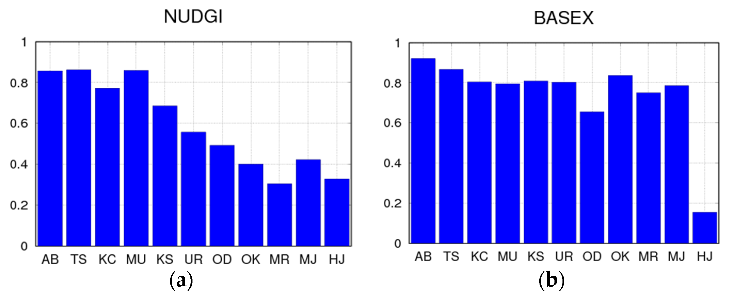
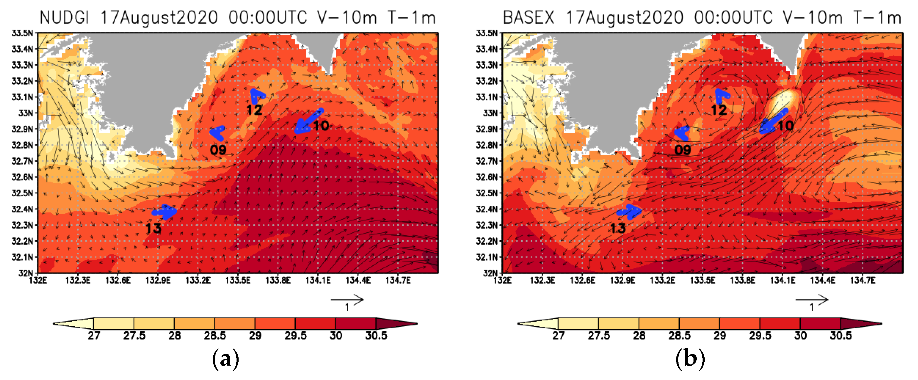
3.1. Effects of the Direct DA Approach (Category 0 Experiments)

Figure 4 compares daily SST snapshots of the previous version JCOPE-T (NUDGI, left) and the base case of JCOPE-T DA (BASEX, right). Although both cases generally represent the observed oceanic conditions (Figure 2), including the Kuroshio large meander south of Japan (Figure 4a,b), the horizontal gradient of SST in Japan Sea and east of Japan (Figure 4c,d), and typhoon-induced SST reduction in the East China Sea (Figure 4c,d), the NUDGI case seemed to represent more smoothed SST distributions compared to the BASEX case. A comparison of the current version (Figure 4d) and the merged satellite SST (Figure 2b), however, suggests that the current version exaggerated the horizontal gradients of the observed SST or represented some streaks not evident in the observation. Later, we discuss parameter sensitivity to these unrealistic aspects. Minimum values of the daily correlation between modeled and observed SSTs during the target period (

Table 2. Minimum values of regionally calculated daily correlation between modeled and observed SST ($SS{T}_o$ ) data for the period from 1 July to 31 August 2020. Locations of the target regions (SOJ: south of Japan, JSS: Japan Sea south, EOJ: east of Japan, ECS: East China Sea) are shown in Figure 1.

Cases	SOJ	JSS	EOJ	ECS
NUGDI	0.65	0.61	0.90	0.79
BASEX	0.67	0.60	0.94	0.79
MGSST	0.53	0.54	0.91	0.61
EXLMS	0.67	0.61	0.94	0.77
SSTSL	0.72	0.65	0.95	0.81
SSTER	0.65	0.60	0.94	0.79
IAUSM	0.66	0.58	0.93	0.79
200KM	0.61	0.60	0.94	0.79
SUMM3	0.72	0.62	0.94	0.80
SSHER	0.71	0.62	0.94	0.80
INSTS	0.71	0.62	0.94	0.80
INTS2	0.70	0.62	0.94	0.80
LOCVL	0.72	0.62	0.94	0.80

) indicated no significant improvements for the base case (BASEX) compared with the previous version (NUDGI), suggesting that the unrealistic streaks patterns affect the daily correlation. This also shows that the improvements in the output quality for the daily correlation of SST in both cases was not very significant (Table 2), but the other model quality metrics showed more significant improvements (

Table 3. Regionally calculated RMSD (in °C) between modeled and observed GTSPP temperature data at 0–100 m depths for the period from 1 July to 31 August 2020. Locations of the observed temperature data are shown in Figure 11a.

Cases	SOJ	JSS	EOJ	ECS
NUGDI	1.6	1.9	2.8	1.1
BASEX	1.4	1.8	2.5	1.0
MGSST	1.6	2.0	2.6	1.1
EXLMS	1.5	1.8	2.5	1.0
SSTSL	1.4	1.7	2.6	1.0
SSTER	1.4	1.8	2.4	1.0
IAUSM	1.4	1.7	2.6	1.0
200KM	1.4	1.8	2.5	1.0
SUMM3	1.4	1.6	2.7	1.0
SSHER	1.4	1.6	2.8	1.0
INSTS	0.9	0.9	1.9	0.7
INTS2	0.9	0.9	1.9	0.7
LOCVL	0.9	0.9	1.9	0.7

, the third column of

Table 4. As in Table 3, except for the observed data locations. “Ship” means the data obtained from the research vessel “Tosa Kaiyou Maru” (see Figure 11b for data locations), and “Buoys” means the data measured at the mooring buoys (No. 09, 10, 12, 13) around Tosa Bay (see Figure 8 for the locations).

Cases	Ship	Buoys
NUGDI	1.5	1.5
BASEX	1.5	0.9
MGSST	1.7	1.1
EXLMS	1.6	1.0
SSTSL	1.6	1.0
SSTER	1.5	0.9
IAUSM	1.5	1.0
200KM	1.5	1.0
SUMM3	1.6	1.0
SSHER	1.6	1.0
INSTS	0.8	1.0
INTS2	0.8	1.0
LOCVL	0.8	0.9

,

Table 5. Correlation (2nd and 4th columns) and RMSD (in m/s, 3rd and 5th columns) between modeled and observed velocity data at 0–100 m depths for the period from July 1 to August 31, 2020. The observed locations were the same as those of temperature data (Table 4). Correlation and RMSD for the velocity data were calculated for all scalar values composed of east–west (u) and north–south (v) components, e.g., $\begin{array}{cc}RMSD=& \sqrt{\frac{1}{2N}{\displaystyle \sum _{i=1}^N\left({(u_i^a-u_i^o)}^2+{(v_i^a-v_i^o)}^2\right)}}\end{array}$ where N denotes the number of the u/v data, “a” and “o” denote modeled and observed velocities, respectively.

Cases	Ship	Ship(m/s)	Buoys	Buoys(m/s)
NUGDI	0.40	0.20	0.02	0.27
BASEX	0.45	0.19	0.26	0.29
MGSST	0.44	0.19	0.32	0.28
EXLMS	0.42	0.20	0.31	0.29
SSTSL	0.43	0.20	0.30	0.28
SSTER	0.46	0.19	0.27	0.29
IAUSM	0.48	0.19	0.30	0.29
200KM	0.39	0.20	0.24	0.29
SUMM3	0.47	0.19	0.26	0.27
SSHER	0.49	0.19	0.26	0.28
INSTS	0.45	0.20	0.31	0.27
INTS2	0.42	0.20	0.31	0.28
LOCVL	0.47	0.21	0.34	0.28

and

Table 6. Latitudinal RMSD (in degrees) between modeled and observed Kuroshio axis positions (see Figure 5 and Figure 12 for the examples) in a longitudinal range of 130° E–140° E for the period from 1 July to 31 August 2020 (KPATH: 2nd column), and mean correlation at the 11 tide gauge sites between modeled and observed sea level anomaly data for the same period. (SLA: 3rd column).

Cases	KPATH	SLA
NUGDI	0.46	0.60
BASEX	0.40	0.74
MGSST	0.39	0.73
EXLMS	0.39	0.77
SSTSL	0.40	0.71
SSTER	0.39	0.72
IAUSM	0.40	0.72
200KM	0.42	0.72
SUMM3	0.38	0.72
SSHER	0.38	0.72
INSTS	0.39	0.65
INTS2	0.38	0.67
LOCVL	0.40	0.65

, and Figure 5).

A typical view of the Kuroshio path locations represented by BASEX (Figure 6b) exhibited JCOPE-T DA represented a complicated shape of the Kuroshio path south of Japan well, as observed, whereas the NUDGI case failed to represent it (Figure 6a). At this time (August 17, 2020), the latitudinal RMSD with the observed Kuroshio path locations in the BASEX case was smaller than that in the NUDGI case (Figure 5). In addition, more complicated horizontal variations shown in SSH (e.g., three cold eddy cores) within the nearshore side of the Kuroshio Large Meander were represented by the BASEX case (Figure 6b) compared with the smoother SSH distribution of NUDGI (Figure 6a).

Comparison of Figure 6a,b further indicates the relatively smaller horizontal scale SSH patterns around the coasts of Japan, including insides of coastal bays (Figure 6a), were changed by applying the daily-basis DA (Figure 6b). Correlation values with the sea level anomaly data were higher at sites in the eastern part of the southern coasts (Figure 3) in the BASEX case (Figure 7; also see Table 6). However, a site on the far offshore side of the Kuroshio path (HJ; see Figure 3 for the location) showed the decline of the skills in the BASEX case (Figure 7). It seemed a bit difficult to reproduce a small-scale range of about 10 cm amplitude associated with smaller/shorter scale variations at HJ (not shown), while at the other 10 sites, the BASEX case reproduced larger-scale variations mainly caused by the Kuroshio path variations well.

The changes in the horizontal gradients of SSH near the coasts affected the representation of the coastal current variations. Figure 8 compares a zoom-up view of ocean current distributions around Tosa Bay in the cases of NUDGI (Figure 8a) and BASEX (Figure 8b). A northward deviation of the Kuroshio front from the observed position southeast of Tosa Bay in the NUDGI case (Figure 6a) led to the prevailing northeastward currents south of Tosa Bay (Figure 8a) but the observed current at a buoy No. 10 indicated a southwestward direction at this time. The BASEX case showed a significant change in the ocean current distribution around Tosa Bay (Figure 8b) and represented the southwestward current around buoy No. 10, as observed. A current direction at buoy No. 13 was changed from eastward (NUDGI) to southwestward (BASEX) and was the opposite to the observed direction.

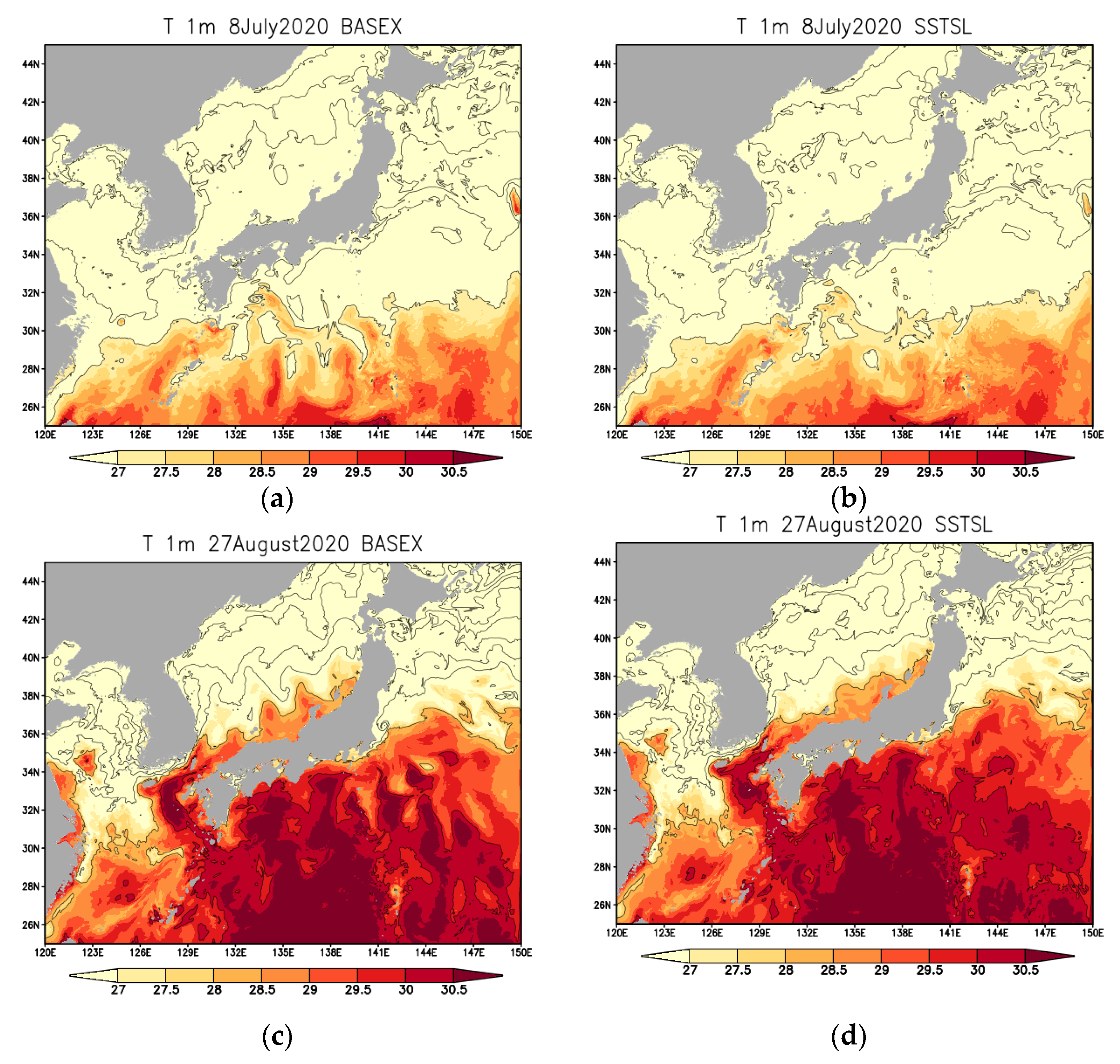
3.2. Effects of Assimilating the Merged Satellite SST (Category 1 Experiments)

The passage of a typhoon frequently causes cooling of the SST through wind-induced vertical mixing and upwelling of the subsurface waters [34]. The satellite merged SST actually detected this weather-induced reduction in SST in the target period (Figure 2b). The reduction in SST was not well represented in the MGDSST case as indicated by the positive biases compared to BASEX shown around 32° N 126° E. (Figure 9a), and the EXLMS case also showed a similar and moderated SST bias (Figure 9b). Both MGSST and EXLMS resulted in a certain positive bias to the observed SST in the ECS region (see Figure 1 for the location of the target area) for the typhoon season, 25 to 31 August 2020, and BASEX reasonably showed a zero bias (

Table 7. Mean difference (in °C) in the ECS region (see Figure 1 for the location) between modeled and observed SST (the merged satellite SST) data the period from August 25 to 31, 2020.

Cases	BIAS
BASEX	0.00
MGSST	0.62
EXLMS	0.16

).

The skill metrics based on the independent TS data (Table 3 and Table 4) indicated a certain decline of the accuracy of the MGSST case, suggesting that the assimilation of the merged satellite SST (${\mathrm{SST}}_{\mathrm{o}}$) works well for better representing the subsurface TS profiles. The EXLMS case also showed a similar decline of the skills as compared to the BASEX case.

3.3. Parameters Sensitivity of the DA Scheme (Category-2 Experiments)

To mitigate the streak patterns of SST shown in the BASEX case, we examined the effects of the several different choices in parameter changes, as described in Section 2.5. Table A1 summarizes all parameters examined in the sensitivity experiments. We found that the most critical parameter associated with the streak patterns was the horizontal scale separation parameter Sc (Equation (A4)). Figure 10 demonstrates that the streak patterns (Figure 10a,c) basically disappeared in the SSTSL case (Figure 10b,d). The minimum correlation of the daily data during the target period certainly increased due to this parameter change (Table 2). Some of the other parameter changes: SSTER and IAUSM, resulted in slight improvements in the metrics (Table 3, Table 5 and Table 6). However, a larger horizontal scale for the larger-scale 3dVar background covariance (the 200 KM case) did not improve nearly any of the skill metrics. To expect combined effects of the “positive” parameter changes except for the parameter changed in the 200 KM case, we conducted an additional sensitivity experiment, including the three parameter changes (SUMM3: SSTSL + SSTER + IAUSM; see Table A1 for the changed parameters), which actually led to some accuracy improvements, as described in Table 2, Table 3, Table 5 and Table 6.

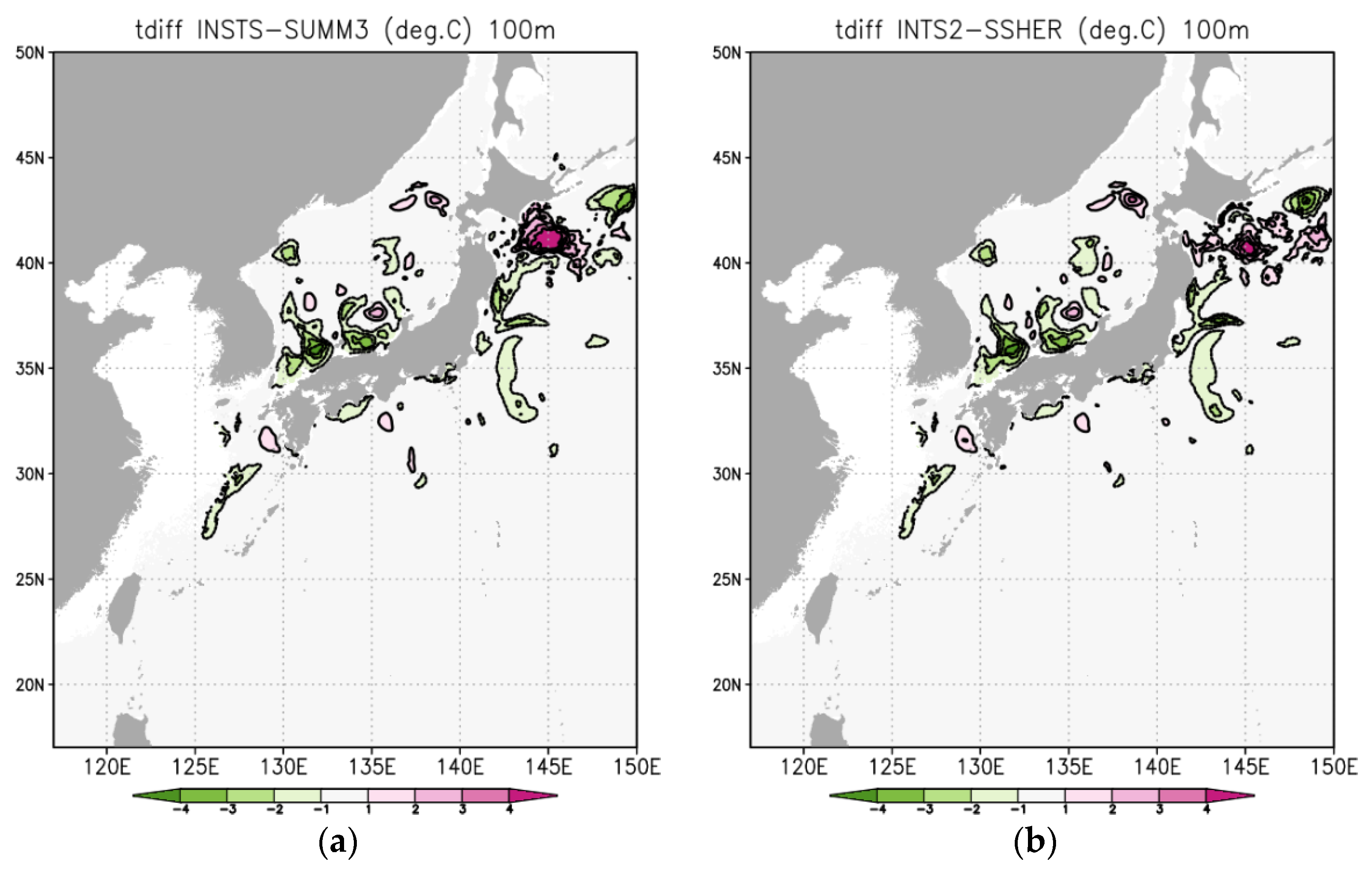
3.4. Sensitivity of Assimilating In situ Temperature/Salinity/Ocean Current Data in Addition to Remote Sensing Data (Category 3 Experiments and an Additional Category 2 Experiment)

We examined the DA impacts of the in situ TS data using a result of a sensitivity experiment (INSTS) which additionally assimilated the in situ TS data into the SUMM3 case, which assimilated the only remote-sensing data. The INSTS case assimilated two different data sources: those archived in GTSPP (see Figure 11a for data locations) and those obtained by the Kochi Prefecture Fishery Agency (see Figure 11b for data locations). The second and third terms of the cost functions Equations (A1) and (A2) were activated in the INSTS case. Table 3 and Table 4 reasonably indicate the expected reduction in RMSD for the assimilated data, though other metrics showed somewhat complicated responses.

Figure 12 shows that the SSH gradients along the coasts were significantly changed by the additional assimilation of the in situ TS data. The modification of the subsurface temperature and salinity changed the distribution of surface dynamic height through changes in the density structure [35]. Actually, changes shown in subsurface temperature at 100 m (Figure 13a) indicated a lower temperature patch inside Tosa Bay. This change was related to the depression of SSH along the coasts (Figure 12). Such additional features were basically interpreted as improvements in the water mass property in the nearshore areas. It is difficult to obtain accurate remote-sensing measurements of SSHA near the coast [36]. For this reason, the SSHA satellite data near the coasts likely contained much “noise”, and, therefore, we did not assimilate any of the SSHA coastal data for water depths shallower than 200 m. In such shallow regions, the assimilation of SST and in situ TS data was required and was effective for the accurate estimation of the oceanic states.

Figure 13a also shows a patch of positive bias around 42° N 144° E in an offshore area. This was because a warm eddy was not reproduced in the SUMM3 case (Figure 14a), though the satellite SSHA data detected a positive anomaly associated with the warm eddy in this period (not shown). To mitigate such unexpected sensitivity to the assimilation of the in situ TS data, we conducted an additional sensitivity experiment (“TSEOF”) using a different statistical dataset for the vertical projection of the remote-sensing data (EOF-B instead of EOF-A; see Appendix A) and a slight reduction in SSH observational error constant value $Er{r}_{SSHA}^o$ (0.10 m–0.07 m; see Equation (A5)) in the region 39.5° N–45° N and 140° E–150° E. Both the original and modified versions of the EOF modes were calculated from the same in situ TS data archive, World Ocean Database 2013 [37], but the locations of the former and latter data sampling were slightly different (Appendix A). Figure 14b demonstrates that the use of the different statistical data extracts the information in a mesoscale eddy from remote-sensing data alone even without the assimilation of the subsurface in situ TS data. The increase in the sampled TS data amount in the wider regions may result in a better representation of the warm eddy by using the EOF modes. Although RMSD for the subsurface temperature increased slightly in the east of Japan in the SSHER case (Table 3), we considered that the warm eddy should be represented with the use of the remote-sensing data alone (cf. Figure 14a,b).

Further comparison of the two sensitivity experiments assimilating the in situ TS data based on SUMM3 (INSTS, Figure 14c) and SSHER (INTS2, Figure 14d) suggested that the use of different statistical data in the SSHER case reproduced the warm eddy well as indicated by the relatively warm temperature observed around the same location. Changes detected in subsurface temperature at 100 m between the INTS2 and SSHER cases (Figure 13b) were more moderated around this location compared with the changes between the INSTS and SUMM3 cases (Figure 13a). Note that the SSHER case also reduced the SSH observation error in a southern region of the Japan Sea (34° N–41° N and 127° E–142° E) from 0.1 to 0.07 m but showed no significant sensitivity in the Japan Sea (Figure 13). Comparison of subsurface temperature distributions between the INSTS and SUMM3 cases in the Japan Sea suggests that additional assimilation of the in situ TS data strengthens the horizontal gradients of the water mass structures of oceanic fronts and eddies (not shown).

Modification of the water mass properties and resulting changes in the SSH gradients in the nearshore regions by assimilating the in situ TS data affected the surface ocean currents in the nearshore region (cf. Figure 15a,b). The eastward direction of the current at the location of buoy No. 13 was partly reproduced in the INSTS case. The subsurface ocean current distribution was also changed by the assimilation of the in situ TS data, as shown in Figure 16a,b. A southwestward current along the coast in Tosa Bay was reproduced in the INSTS case, as observed.

The last case of sensitivity experiments (LOCVL) was performed for investigating the impacts of assimilating the ocean current velocity data distributed in a localized nearshore region (see Figure 11b for data locations). The assimilation changed the oceanic conditions inside of Tosa Bay (cf. Figure 15b,c). The most significant sensitivity by assimilating the ocean current velocity data is illustrated in Figure 16b,c. The data covering a wide range from nearshore to offshore sides effectively modified the simulated ocean current distribution. The intensity of the southwestward current was enhanced by the assimilation of the velocity data, and the horizontal shear of the ocean current became more similar to the observed shear distribution. In addition, the skills for the not-assimilated (buoys) and assimilated (ship) data were slightly improved (Table 5).

4. Discussion

The model validation using the skill metrics based on the independent observational data clearly demonstrated that JCOPE-T DA based on the direct DA approach outperformed the previous version of JCOPE-T based on the indirect DA approach. The quality of the model output based on the indirect DA approach depended on the reference DA products, e.g., JCOPE2M. The improved model output is attributed to the direct DA approach adopted in JCOPE-T DA. The direct DA approach allows: (1) the higher horizontal resolution of the first guess model (1/36 degree) than that of JCOPE2M (1/12 degree), (2) a shorter time window of the daily-updated satellite SST data (2 days) as compared to 4 days applied to JCOPE2M, and (3) a shorter IAU time scale (1 day) preserving a few days’ scale variation compared to 4 days IAU time scale in JCOPE2M.

The sensitivity experiment assimilating the temporally and spatially smoothed SST data (the MGDSST case) suggests that the assimilation of the daily-updated satellite SST effectively works for representing few-day scale phenomena caused by a typhoon. The other sensitivity experiments indicate that the choice of the parameter for separation of the horizontal scale $S_C$ (Equation (A4)) is strongly related to the appearance of the streak’s patterns in the model SST. We found that minimization of the small-scale cost function (Equation (A3)) with $S_C$ = 50 km (BASEX) required considerably more iterations over 100 times than that in the case with $S_C$ = 150 km (SSTSL). The resulting small-scale analysis increment ($\delta X_S^a$) of SST in the BASEX case involved unrealistic noisy patches, while they disappeared in the SSTSL case (not shown). The small-scale features, including some noises contained in the observed SST data, were exaggerated in the small-scale analysis increment in the BASEX case by overfitting them.

To summarize, we know that the additional assimilation of the in situ TS data changed the water mass structure, especially in the nearshore areas. The in situ TS DA also changed the horizontal gradients of SSH near the coasts, and thereby, the ocean current distributions were changed through geostrophic adjustment responding to the changes in the SSH distribution. The further additional assimilation of the ADCP ocean current data revealed that the ocean current distribution was reasonably corrected around Tosa Bay by including the information from the in situ ADCP data. The accuracy of the remote-sensing data (SST and SSHA) deteriorated near the coasts due to various kinds of noises [26,35]. The sensitivity experiments suggest that the assimilation of the in situ data in addition to the remote-sensing data effectively works for correctly representing the oceanic conditions around Tosa Bay.

This study suggests the remaining unresolved issues: (1) the correlation for the currents measured at the buoys around Tosa bay was not high, (2) the additional assimilation of in situ data resulted in a slight decline in the skills at representing the sea level variations at the tide gauge sites, (3) full potential of high-resolution (<500 m) SST has still not been explored, and (4) forecasting skills for the 10 day lead forecast period was out of scope for this study. We should continue to make various efforts for improving the skills of the model products, including developments of downscaled ocean models with horizontally/vertically higher resolution and more advanced DA methods.

5. Conclusions

We constructed an OSF system, JCOPE-T DA, based on the daily-basis assimilation of remote-sensing data. The validation in the present study demonstrated that DA on a daily basis effectively estimates the oceanic phenomena with a few days’ time scale around the Japan coastal ocean. All updating procedures are automated and daily-updated 10-day lead forecast information is visualized on a website: https://www.eorc.jaxa.jp/ptree/ocean_model/index.html (accessed on 19 June 2021)

A close collaboration between space remote-sensing and ocean research groups contributes to the development and maintenance of the daily-updated OSF system.

This study has considerably improved the accuracy of our oceanic model through daily assimilation of in situ data in addition to assimilating the remote-sensing data. At the present time, the JCOPE-T DA system is downloading the in situ TS data from the GTSPP archive [25], which accumulates the in situ TS data after receiving various kinds of data sources obtained by the ARGO floats, research vessels, and buoys. The accumulation of the in situ data is basically delayed as compared with the timing of actual measurements. Most of the oceanographic sensors are not directly connected to the internet, so the data has to be transmitted manually. This slows down the entire process. However, recently, there has been significant development of in situ oceanographic sensors that are directly and automatically connected to the internet (e.g., [38,39]). This tendency is considered as a part of the ongoing development of “Internet of Things technology”, which enables computers to observe, identify, and understand the oceanic states without the limitations of human-entered data [40]. The close collaboration between ocean modeling and in situ observation groups should be enhanced and extended to include more real-time acquisition of the in situ data along this trend currently in progress.

References

1. Ezer, T.; Mellor, G.L. Continuous assimilation of Geosat altimeter data into a primitive equation Gulf Stream model. J. Phys. Oceanogr. 1994, 2, 832–847. [Google Scholar] [CrossRef]
2. Ezer, T.; Mellor, G.L. Data assimilation experiments in the Gulf Stream region: How useful are satellite-derived surface data for nowcasting the subsurface field? J. Atmos. Ocean Tech. 1997, 14, 1379–1391. [Google Scholar] [CrossRef]
3. Fujii, Y.; Kamachi, M. A reconstruction of observed profiles in the sea east of Japan using vertical coupled temperature-salinity EOF modes. J. Oceanogr. 2003, 59, 173–186. [Google Scholar] [CrossRef]
4. Bell, M.J.; Schiller, A.; Le Traon, P.Y.; Smith, N.R.; Dombrowsky, E.; Wilmer-Becker, K. An introduction to GODAE Ocean View. J. Oper. Oceanogr. 2015, 8, s2–s11. [Google Scholar]
5. Hirose, N.; Usui, N.; Sakamoto, K.; Tsujino, H.; Yamanaka, G.; Nakano, H.; Urakawa, S.; Toyoda, T.; Fujii, Y.; Kohno, N. Development of a new operational system for monitoring and forecasting coastal and open-ocean stats around Japan. Ocean Dyn. 2019, 69, 1333–1357. [Google Scholar] [CrossRef]
6. Usui, N.; Fujii, Y.; Sakamoto, K.; Kamachi, M. Development of four-dimensional variational assimilation system for coastal data assimilation around Japan. Mon. Weather Rev. 2015, 143, 3874–3892. [Google Scholar] [CrossRef]
7. Miyazawa, Y.; Murakami, H.; Miyama, T.; Varlamov, S.M.; Guo, X.; Waseda, T.; Sil, S. Data assimilation of the high-resolution sea surface temperature obtained from the Aqua-Terra satellites (MODIS-SST) using an ensemble Kalman filter. Remote Sens. 2013, 5, 3123–3139. [Google Scholar] [CrossRef] [Green Version]
8. Sakamoto, K.; Tsujino, H.; Nakano, H.; Hirabara, M.; Yamanaka, G. A practical scheme to introduce explicit tidal forcing into an OGCM. Ocean Sci. 2013, 9, 1089–1108. [Google Scholar] [CrossRef] [Green Version]
9. Varlamov, S.M.; Guo, X.; Miyama, T.; Ichikawa, K.; Waseda, T.; Miyazawa, Y. M2 baroclinic tide variability modulated by the ocean circulation south of Japan. J. Geophys. Res. Oceans 2015, 120, 3681–3710. [Google Scholar] [CrossRef]
10. Miyazawa, Y.; Kagimoto, T.; Guo, X.; Sakuma, H. The Kuroshio large meander formation in 2004 analyzed by an eddy-resolving ocean forecast system. J. Geophys. Res. Oceans 2008, 113, C10015. [Google Scholar] [CrossRef] [Green Version]
11. Miyazawa, Y.; Zhang, R.C.; Guo, X.; Tamura, H.; Ambe, D.; Lee, J.S.; Okuno, A.; Yoshinari, H.; Setou, T.; Komatsu, K. Water mass variability in the Western North Pacific detected in a 15-year eddy resolving ocean reanalysis. J. Oceanogr. 2009, 65, 737–756. [Google Scholar] [CrossRef]
12. Miyazawa, Y.; Varlamov, S.M.; Miyama, T.; Guo, X.; Hihara, T.; Kiyomatsu, K.; Kachi, M.; Kurihara, Y.; Murakami, H. Assimilation of high-resolution sea surface temperature data into an operational nowcast/forecast system around Japan using a multi-scale three-dimensional variational scheme. Ocean Dyn. 2017, 67, 713–728. [Google Scholar] [CrossRef]
13. Donlon, C.; Robinson, I.; Casey, K.S.; Vazquez-Cuervo, I.; Armstrong, E.; Arino, O.; Gentermann, C.; May, D.; LeBorgne, P.; Piolle, J.; et al. The Global Ocean Data Assimilation Experiment High-resolution Sea Surface Temperature Pilot Project. Bull. Amer. Met. Soc. 2007, 88, 1197–1214. [Google Scholar] [CrossRef]
14. Mellor, G.L.; Hakkinen, S.; Ezer, T.; Patchen, R. A generalization of a sigma coordinate ocean model and an inter comparison of model vertical grids. In Ocean Forecasting: Conceptual Basis and Applications; Pinardi, N., Woods, J.D., Eds.; Springer: New York, NY, USA, 2002; pp. 55–72. [Google Scholar]
15. Nakanishi, M.; Niino, H. Development of an improved turbulence closure model for the atmospheric boundary layer. J. Metorol. Soc. Jpn. 2009, 87, 895–912. [Google Scholar] [CrossRef] [Green Version]
16. Furuichi, N.; Hibiya, T.; Niwa, Y. Assessment of turbulence closure models for resonant inertial response in the oceanic mixed layer using a large eddy simulation model. J. Oceanogr. 2012, 68, 285–294. [Google Scholar] [CrossRef]
17. Li, Y.; Gao, Z.; Lenschow, D.H.; Chen, F. An improved approach for parameterizing surface layer turbulent transfer coefficients in numerical models. Bound. Layer Meteorol. 2010, 137, 153–165. [Google Scholar] [CrossRef] [Green Version]
18. Lindau, R. Climate Atlas of the Atlantic Ocean; Springer: Berlin/Heidelberg, Germany, 2001. [Google Scholar]
19. Malevskii, S.P.; Girduc, G.V.; Egorov, B. Radiation Balance of the Ocean Surface; Gidrometeoizdat: Sankt-Petersburg, Russia, 1992. [Google Scholar]
20. Payne, R.E. Albedo of the sea surface. J. Atmos. Sci. 1972, 29, 959–970. [Google Scholar] [CrossRef]
21. Paulson, C.A.; Simpson, J.J. Irradiance measurements in the upper ocean. J. Phys. Oceanogr. 1977, 7, 952–956. [Google Scholar] [CrossRef]
22. Clark, N.E.; Eber, L.; Laurs, R.M.; Renner, A.; Saur, J.F.T. Heat Exchange between Ocean and Atmosphere in the Eastern North Pacific for 1961–71; NOAA Tech. Rep. NMFS SSRF-682; US Department of Commerce: Washington, DC, USA, 1974.
23. Egbert, G.D.; Erofeeva, S.Y. Efficient inverse modeling of barotropic ocean tides. J. Atmos. Ocean. Technol. 2002, 19, 183–204. [Google Scholar] [CrossRef] [Green Version]
24. Bloom, S.C.; Takacs, L.L.; da Silva, A.M.; Ledvina, D. Data assimilation using Increment Analysis Updates. Mon. Weather Rev. 1996, 124, 1256–1271. [Google Scholar] [CrossRef] [Green Version]
25. Sun, C.; Thresher, A.; Keely, R.; Hall, N.; Hamilton, M.; Chinn, P.; Tran, A.; Goni, G.; Petit de la Villeon, L.; Carval, T.; et al. The data management system for the Global Temperature and Salinity Profile Programme. In Proceedings of the OceanObs.09: Sustained Ocean Observations and Information for Society, Venice, Italy, 21–25 September 2009. [Google Scholar]
26. Shibata, A. AMSR/AMSR-E SST algorithm developments; removable of ocean wind effect. Ital. J. Remote Sens. 2004, 30/31, 131–142. [Google Scholar]
27. Kurihara, Y.; Murakami, H.; Kachi, M. Sea surface temperature from the new Japanese geostationary meteorological Himawari-8 satellite. Geophys. Res. Lett. 2016, 43, 1234–1240. [Google Scholar] [CrossRef] [Green Version]
28. Kurihara, Y.; Murakami, H.; Ogata, K.; Kachi, M. A quasi-physical sea surface temperature method for the split-window data from the Second-generation Global Imager (SGLI) onboard the Global Change Observation Mission-Climate (GCOM-C) satellite. Remote Sens. Environ. 2021, 257, 112347. [Google Scholar] [CrossRef]
29. Xu, F.; Ignatov, A. In situ SST Quality Monitor (iQuam). J. Atmos. Ocean. Tech. 2014, 31, 164–180. [Google Scholar] [CrossRef]
30. Kawabe, M. Sea level changes south of Japan associated with the non-large-meander path of the Kuroshio. J. Oceanogr. Soc. Jpn. 1989, 45, 181–189. [Google Scholar] [CrossRef]
31. Hanawa, K.; Mitsudera, H. About the daily averaging method of oceanic data. Bull. Coast. Oceanogr. 1985, 23, 79–87. [Google Scholar]
32. Miyazawa, Y.; Guo, X.; Varlamov, S.M.; Miyama, T.; Yoda, K.; Sato, K.; Kano, T.; Sato, K. Assimilation of the sea bird and ship drift data in the north-eastern sea of Japan into an operational ocean nowcast/forecast system. Sci. Rep. 2016, 5, 17672. [Google Scholar] [CrossRef] [PubMed] [Green Version]
33. Kurihara, Y.; Sakurai, T.; Kuragano, T. Global daily sea surface temperature analysis using data from satellite microwave radiometer, satellite infrared radiometer and in-situ observations. Weather Bull. 2006, 73, s1–s18. [Google Scholar]
34. Kanada, S.; Tsujino, S.; Aiki, H.; Yoshida, K.M.; Miyazawa, Y.; Tsuboki, K.; Takayabu, I. Impacts of SST patterns on rapid intensification of typhoon Megi (2010). J. Geophys. Res. Atmos. 2017, 122, 13245–13262. [Google Scholar] [CrossRef] [Green Version]
35. Kuragano, T.; Shibata, A. Sea surface dynamic height of the Pacific Ocean derived from TOPEX/POSEIDON altimeter data: Calculation method and accuracy. J. Oceanogr. 1997, 53, 585–599. [Google Scholar]
36. Xu, X.-Y.; Birol, F.; Cazenave, A. Evaluation of coastal sea level offshore Hong Kong from Jason-2 altimetry. Remote Sens. 2017, 10, 282. [Google Scholar] [CrossRef] [Green Version]
37. Boyer, T.P.; Antonov, J.I.; Baranova, O.K.; Coleman, C.; Garcia, H.E.; Grodsky, A.; Johnson, D.R.; Locarnini, R.A.; Mishonov, A.V.; O’Brien, T.D.; et al. World Ocean Database 2013; NOAA Atlas NESDIS 72; NOAA: Washington, DC, USA, 2013.
38. Nakada, S.; Hirose, N.; Senjyu, T.; Fukudome, K.; Tsuji, T.; Okei, N. Operational ocean prediction experiments for smart coastal fishing. Prog. Oceanogr. 2014, 121, 125–140. [Google Scholar] [CrossRef]
39. Takikawa, T.; Kanetake, M.; Itou, T.; Hirose, N. Hydrographic observations by fisherman and coastal ocean model—Salinity variations around Iki Island during cooling season. J. Adv. Mar. Sci. Technol. Soc. 2019, 25, 15–20. [Google Scholar]
40. Ashton, K. That ‘Internet of Things’ Thing. Available online: https://www.rfidjournal.com/that-internet-of-things-thing (accessed on 13 March 2021).
Figure 1. Daily mean SST (in °C) of the SUMM3 case (a best-case of three tuned parameters: SSTSL + SSTER + IAUSM; see Section 3.4 for more deatil) in the JCOPE-T model region on 27 August 2020. Squares denote separated regions for the skill evaluation: East China Sea (ECS), south of Japan (SOJ), east of Japan (EOJ), and the Japan Sea southern region (JSS). The location of Tosa Bay is depicted with “TB.” The black curves with arrows indicate the major ocean currents around Japan’s coasts: Kuroshio (KS), Kuroshio Extension (KE), Tsushima Current (TS), Tsugaru Current (TG), Oyashio (OY), Soya Current (SY).
Remotesensing 13 02431 g001
Figure 2. Daily composite of the merged satellite SST (in °C). Data gaps are represented by blue shading. (a) 8 July 2020, (b) 27 August 2020. The track of the typhoon (BAVI) number 8, 2020 is depicted by a green color curve in (b).
Remotesensing 13 02431 g002
Figure 3. Modeled bottom topography south of Japan (in m, shades). Two letters denote the positions of the tide gauge sites (AB: Aburatsu, TS: Tosa Shimizu, KC: Kochi, MU: Muroto, KS: Kushimoto, UR: Uragami, OD: Ohdomari, OK: Okada, MR: Mera, MJ: Miyakejima, HJ: Hachijojima).
Remotesensing 13 02431 g003
Figure 4. Modeled daily mean SST (in °C). (a,b): 8 July 2020. Solid arrows denote the Kuroshio Large Meander south of Japan, (c,d): 27 August 2020. Solid (dotted) arrows denote the north–south gradient of SST in the Japan Sea and east of Japan (the typhoon-induced SST reduction). (a,c): the NUDGI case, (b,d): the BASEX case.
Remotesensing 13 02431 g004aRemotesensing 13 02431 g004b
Figure 5. Time sequences of daily latitudinal RMSD (in degrees) between the modeled (six cases) and observed Kuroshio axis positions in a longitudinal range of 130° E–140° E. The modeled Kuroshio axis positions were defined as the closest locations to the observed ones with daily mean SSH = 0.3 m.
Remotesensing 13 02431 g005
Figure 6. Daily mean modeled SSH on 17 August 2020. (a) NUDGI case, (b) BASEX case. Blue and black curves denote the locations of the modeled SSH = 0.3 m and observed Kuroshio positions, respectively.
Remotesensing 13 02431 g006
Figure 7. Correlation values between modeled and observed sea level anomaly at the 11 tide gauges sites for the period from 1 July to 31 August 2020(see Figure 3 for the locations). (a) case NUDGI, (b) case BASEX.
Remotesensing 13 02431 g007
Figure 8. Snapshots of the modeled current at 10 m depth (black vectors) and temperature at 1 m depth (color) at 00 17 August 2020, UTC. (a) NUDGI case, (b) BASEX case. Blue vectors denote the current measured at the same time by four mooring buoys.
Remotesensing 13 02431 g008
Figure 9. Difference in SST between the MGSST (a) EXLMS (b) and BASEX cases on 27 August 2020.
Remotesensing 13 02431 g009
Figure 10. Modeled daily mean SST (in °C). (a,b): 8 July 2020. (c,d): 27 August 2020. (a,c): the BASEX case, (b,d): the SSTSL case. Contours denote isotherms with 1 °C interval. The color bar range is determined for visualizing the streaks shown in the BASEX case.
Remotesensing 13 02431 g010
Figure 11. Mean temperature of the INSTS case for the period from 1 July to 31 August 2020. (a) The model region at 100 m depth. (b) Around Tosa Bay at 50 m depth. Open circles denote the locations of temperature observed during the same period archived at GTSPP (a) and provided from Kochi Prefecture Fishery Research Agency (b) with the color shade denoting temperature of the in situ data. Note that the ocean current velocities were also measured at the locations denoted by the open circles shown in (b).
Remotesensing 13 02431 g011
Figure 12. Same as Figure 6 except for (a) the SUMM3 case and (b) the INSTS case.
Remotesensing 13 02431 g012
Figure 13. Mean difference in temperature (in °C) at 100 m depth for the period from 1 July to 31 August 2020 between the INSTS and SUMM3 cases (a) and between the INTS2 and SSHER cases (b).
Remotesensing 13 02431 g013
Figure 14. Mean temperature (in °C) of four cases at 100 m depth for the period from 1 July to 31 August 2020. (a) SUMM3, (b) SSHER, (c) INSTS, (d) INTS2. Open circles denote the locations of temperature observed during the same period, with the color shade denoting temperature of the in situ data.
Remotesensing 13 02431 g014
Figure 15. Same as Figure 8, except for three cases, (a) SUMM3, (b) INSTS, and (c) LOCVL.
Remotesensing 13 02431 g015
Figure 16. Daily mean modeled current at 100 m depth of three cases (black vectors) on 4 August 2020 JST. (a) SUMM3, (b) INSTS, and (c) LOCVL. Blue color vectors denote the observed current obtained by the research vessel Tosa Kaiyou Maru on 4 August 2020 JST.
Remotesensing 13 02431 g016