
Atmospheric Light Estimation Based Remote Sensing Image Dehazing
by
 ,
,
Zhiqin Zhu
1, 
Yaqin Luo
1,
Hongyan Wei
1,
Yong Li
2,
Guanqiu Qi
3,*,
Neal Mazur
3,
Yuanyuan Li
1 and
Penglong Li
4,5 1
College of Automation, Chongqing University of Posts and Telecommunications, Chongqing 400065, China
2
College of Computer Science, Chongqing University, Chongqing 400044, China
3
Computer Information Systems Department, State University of New York at Buffalo State, Buffalo, NY 14222, USA
4
School of Geosciences and Info-Physics, Central South University, Changsha 410083, China
5
Chongqing Geomatics and Remote Sensing Center, Chongqing 401147, China
*
Author to whom correspondence should be addressed.
Remote Sens. 2021, 13(13), 2432; https://0-doi-org.brum.beds.ac.uk/10.3390/rs13132432
Submission received: 26 May 2021
/
Revised: 19 June 2021
/
Accepted: 19 June 2021
/
Published: 22 June 2021
Abstract
:Remote sensing images are widely used in object detection and tracking, military security, and other computer vision tasks. However, remote sensing images are often degraded by suspended aerosol in the air, especially under poor weather conditions, such as fog, haze, and mist. The quality of remote sensing images directly affect the normal operations of computer vision systems. As such, haze removal is a crucial and indispensable pre-processing step in remote sensing image processing. Additionally, most of the existing image dehazing methods are not applicable to all scenes, so the corresponding dehazed images may have varying degrees of color distortion. This paper proposes a novel atmospheric light estimation based dehazing algorithm to obtain high visual-quality remote sensing images. First, a differentiable function is used to train the parameters of a linear scene depth model for the scene depth map generation of remote sensing images. Second, the atmospheric light of each hazy remote sensing image is estimated by the corresponding scene depth map. Then, the corresponding transmission map is estimated on the basis of the estimated atmospheric light by a haze-lines model. Finally, according to the estimated atmospheric light and transmission map, an atmospheric scattering model is applied to remove haze from remote sensing images. The colors of the images dehazed by the proposed method are in line with the perception of human eyes in different scenes. A dataset with 100 remote sensing images from hazy scenes was built for testing. The performance of the proposed image dehazing method is confirmed by theoretical analysis and comparative experiments.

1. Introduction
Remote sensing image retrieval requires quick and accurate search of the targeted areas in a large-scale remote sensing image database. Accuracy, efficiency, and robustness are three important requirements that need to be achieved in the implementation of remote sensing image retrieval [1]. Remote sensing images with high quality and clarity are required. Unfortunately, the acquisition process of remote sensing images highly relies on atmospheric conditions [2]. So, it is difficult to ensure both quality and clarity of a remote sensing image during the acquisition process. The remote sensing images acquired in hazy and foggy scenes are usually subject to both significant contrast reduction and noticeable visibility degradation, which cannot satisfy the basic requirements of remote sensing image retrieval.
Fog, haze, and mist as inevitable natural phenomena not only reduce the effectiveness and practicability of remote sensing image retrieval but also seriously affect aerial photography [3]. Therefore, haze removal plays an irreplaceable role in remote sensing image and aerial photography related applications. However, haze removal (also called dehazing) is underconstrained, when there is only a single hazy image as input [4]. Haze in nature images and remote sensing images is caused by the same or similar physical principles, for example suspending aerosol in the air. Due to various distances of imaging sensors, remote sensing images often have different scene depth estimation. So, the haze removal of remote sensing images needs to train a set of parameters for accurate scene depth estimation.
According to the theoretical basis of image degradation from existing atmospheric scattering models [5], this paper proposes an atmospheric light estimation based scattering model for remote sensing image dehazing. The proposed solution mainly focuses on solving two existing issues, the estimation of atmospheric light and the calculation of a transmission map. First, based on the research of color attenuation prior [6], a linear model is created for scene depth. According to the probability of density distribution, the scene depth map of remote sensing images can be estimated by a distribution function. The optimal parameters of the linear model are first obtained by learning, and then the scene depth information of hazy images is recovered by the learned linear model. According to the obtained scene depth map of a hazy image, the atmospheric light can be estimated. Second, a haze-lines model [7] is built to model a hazy remote sensing image, in which a transmission map is calculated by haze-lines in RGB bands. Finally, according to the estimated atmospheric light and the calculated transmission map, the proposed atmospheric scattering model can effectively achieve remote sensing image dehazing.
The main contributions of this paper are summarized as follows:
- A continuously differentiable function is created to learn the optimal parameters of a linear scene depth model for the scene depth map estimation of remote sensing images.
- A color attenuation and haze-lines-based framework is proposed for the haze removal of remote sensing images, which can effectively achieve image dehazing with little color distortion.
- A haze remote sensing image dataset is created as a benchmark that contains both high- and low-resolution hazy remote sensing images. Experimental results confirm that the proposed solution has good performance on a created image dataset.
2. The Development of Remote Sensing Image Dehazing
As a practical and valuable research topic, existing image dehazing solutions are developed based on both physical and non-physical models [8]. Non-physical model-based dehazing algorithms directly improve image contrast and highlight image details by global or local processing. Mainstream methods of image enhancement include histogram equalization [9], homomorphic filtering [10], wavelet transform [11,12], image fusion [13,14,15], and deep learning [16], which are widely used to improve image contrast to further obtain haze-free images. The above image-enhancement-based dehazing methods only reduce image haze to a certain extent, but they are not applicable to dense haze [17]. As an important evaluation indicator, visibility is used to evaluate the quality of the extracted image features from geographic information systems (GIS), so the visibility enhancement of hazy remote sensing images has already become an important research topic. However, these types of methods in [18,19,20] cannot reliably present satisfactory dehazing results. Physical model-based dehazing algorithms have achieved significant progress in recent years. These algorithms establish mathematical models by understanding the causes of degradation, and recovering related images by means of auxiliary or prior information. The atmospheric scattering model, usually used in dealing with hazy images, is described in RGB bands as follows.
where is the pixel coordinates, I is the observed hazy image, J is the scene radiance representing the haze-free image, is the transmission map, and A is the global atmospheric light that is ambient light scattered by particles in the atmosphere. In Equation (1), the direct attenuation in the first term indicates the scene radiance and its decay in the medium. The second term represents the airlight results from the previously scattered light and leads to a shift of scene colors. In recent years, abundant priors and assumptions [21,22,23,24] have been used to estimate A and t from I. Due to different imaging modes, satellite sensors and conventional cameras have different scattering effects. The size of haze particles is relatively large in the hazy images captured by conventional cameras. However, particles are only visible at the molecular level in the hazy images captured by remote sensing sensors [25,26]. As a color drift phenomenon, pseudo-colors always occur, which cause the loss of natural color rendition. In recent years, many physical model-based dehazing algorithms have been proposed to remove the haze from remote sensing images. Pan [27] presented a deformed haze imaging model to remove haze from remote sensing images. The atmospheric light and transmission are estimated according to this model combined with dark channel prior. Singh [28] proposed an improved restoration model, this model redefined the transmission map and utilized the modified joint trilateral filter to improve estimated atmospheric veil. The algorithms used in these methods are only effective for operation on specific local regions but cannot process a whole image properly [29].
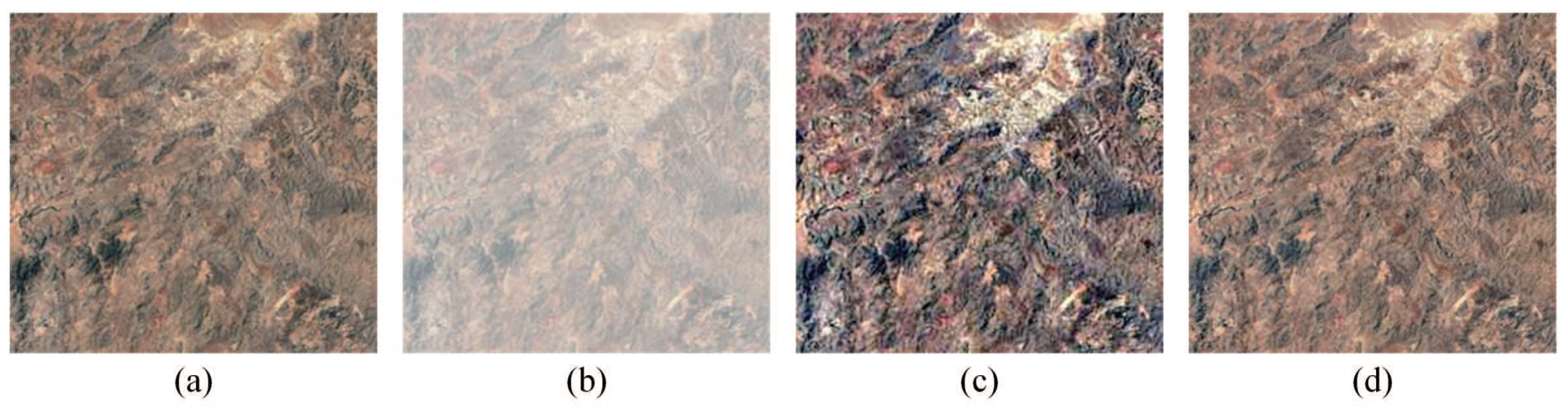
According to the assumption of constant transmission within in a small patch, patch-based methods utilize image priors to avoid the artifacts generated in the dehazing process by overlapping patches [21], building connections between different pixels far from the camera for regularization [30], or using multiple patch sizes [31]. Although existing solutions have made a great improvement in image dehazing, various issues occur in the dehazing process of remote sensing images. There are many differences between hazy remote sensing images and regular hazy images from various natural environments. The haze-lines-based dehazing method proposed by Berman not only estimates atmospheric light, but also calculates transmission maps of hazy images. Haze-lines-based dehazing methods can spread across a whole image, so they can capture global phenomena that are not limited to local image patches [7]. However, due to the color distortion generated during the dehazing process, haze-lines-based methods are not directly applicable to the estimation of atmospheric light and transmission map [7] for remote sensing images. Figure 1 shows a remote sensing image dehazing example. Color distortion caused by a haze-lines-based dehazing method is shown in Figure 1c. Thus, this paper proposes a solution of atmospheric light estimation specialized for remote sensing images to solve the issues of color distortion. As shown in Figure 1d, the proposed method can effectively remove haze from a synthetic hazy image.
3. The Proposed Dehazing Framework for Remote Sensing Images
As shown in Figure 2, a dehazing framework for remote sensing images is proposed, including a linear scene depth estimation model [6]. A linear scene depth estimation model is used to estimate the scene depth map of a hazy remote sensing image. According to the obtained scene depth map, the global atmospheric light is further estimated. Both saturation and brightness information of the original image I is implemented to obtain scene depth information by using the trained parameters. According to the scene depth map d of the original image I, the position information of the top 0.1% of the brightest pixels is estimated [32]. In RGB bands, R, G, and B bands have the corresponding pixel gray values. All the remote sensing images collected by the same satellite (Pleiades A/B) have similar height. The altitude range of the aerosol layer is 2 km, and the irregularity of the aerosol decreases with the increase of altitude. The position of the satellite is higher than 2 km and the corresponding aerosol distribution is regular [33]. According to Berman’s discussion [7] and the relatively uniform spatial distribution of aerosols [33], this paper uses the grayscale pixel value of the R channel as image intensity. The pixel with the highest intensity among all the pixels of the original image I is selected as the global atmospheric light A. The hazy pixels with the same color plotted in RGB bands that pass through A are distributed along lines. Since the transmission map can be estimated by the haze-lines model, the original image I and A are used to redefine the original image I. The redefined image marked as is transformed from RGB bands to spherical coordinates. According to the spherical coordinates, the initial transmission map is estimated. Then regularization is performed to optimize the transmission map. With the obtained global atmospheric light A and transmission map , the dehazed image J can be obtained by the atmospheric scattering model shown in Equation (1).
3.1. Scene Depth Map Restoration
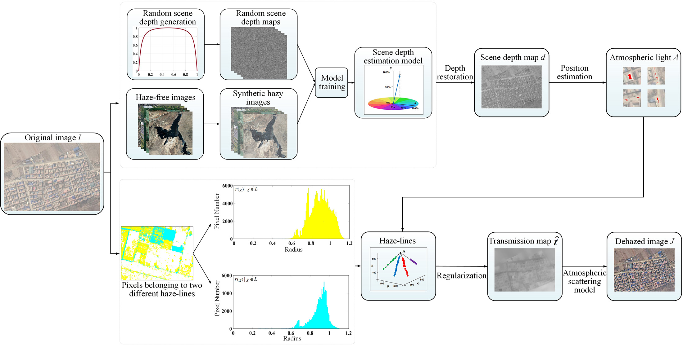
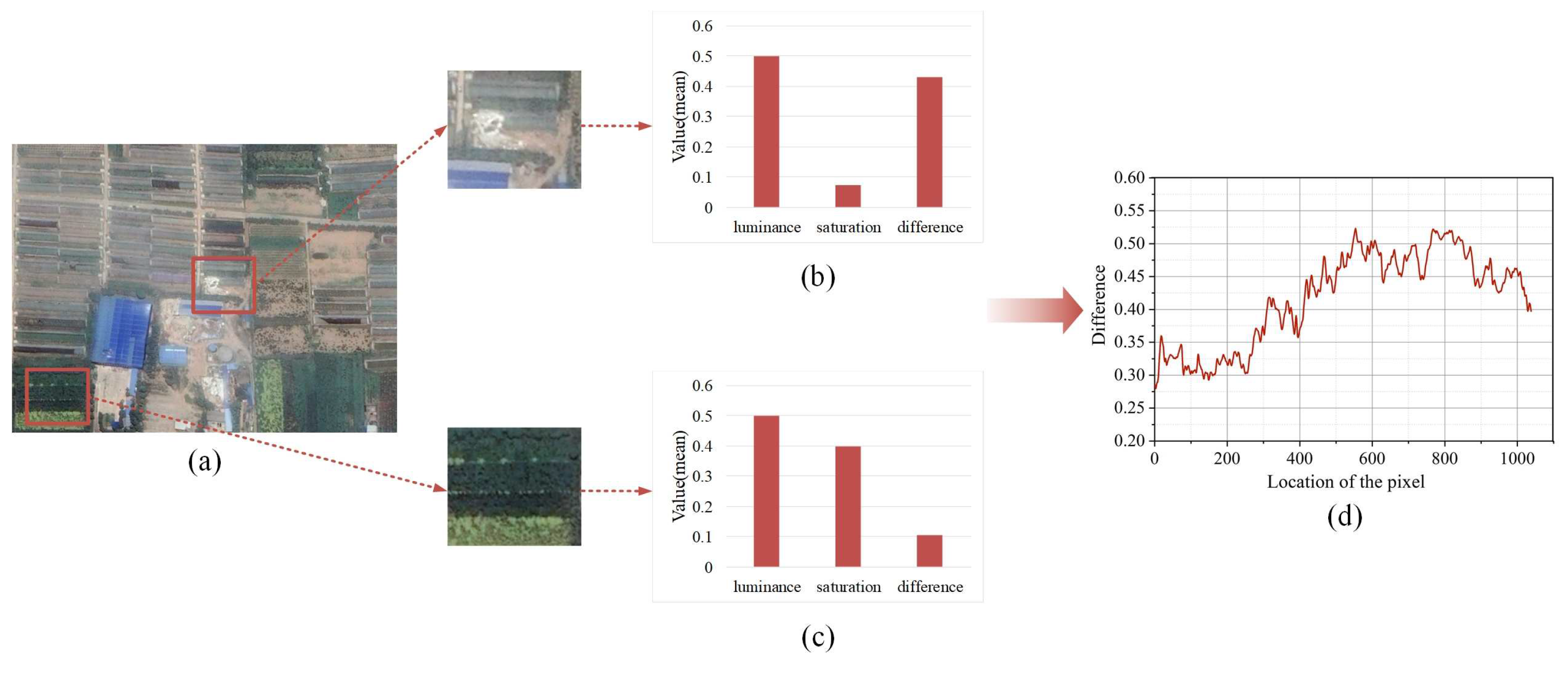
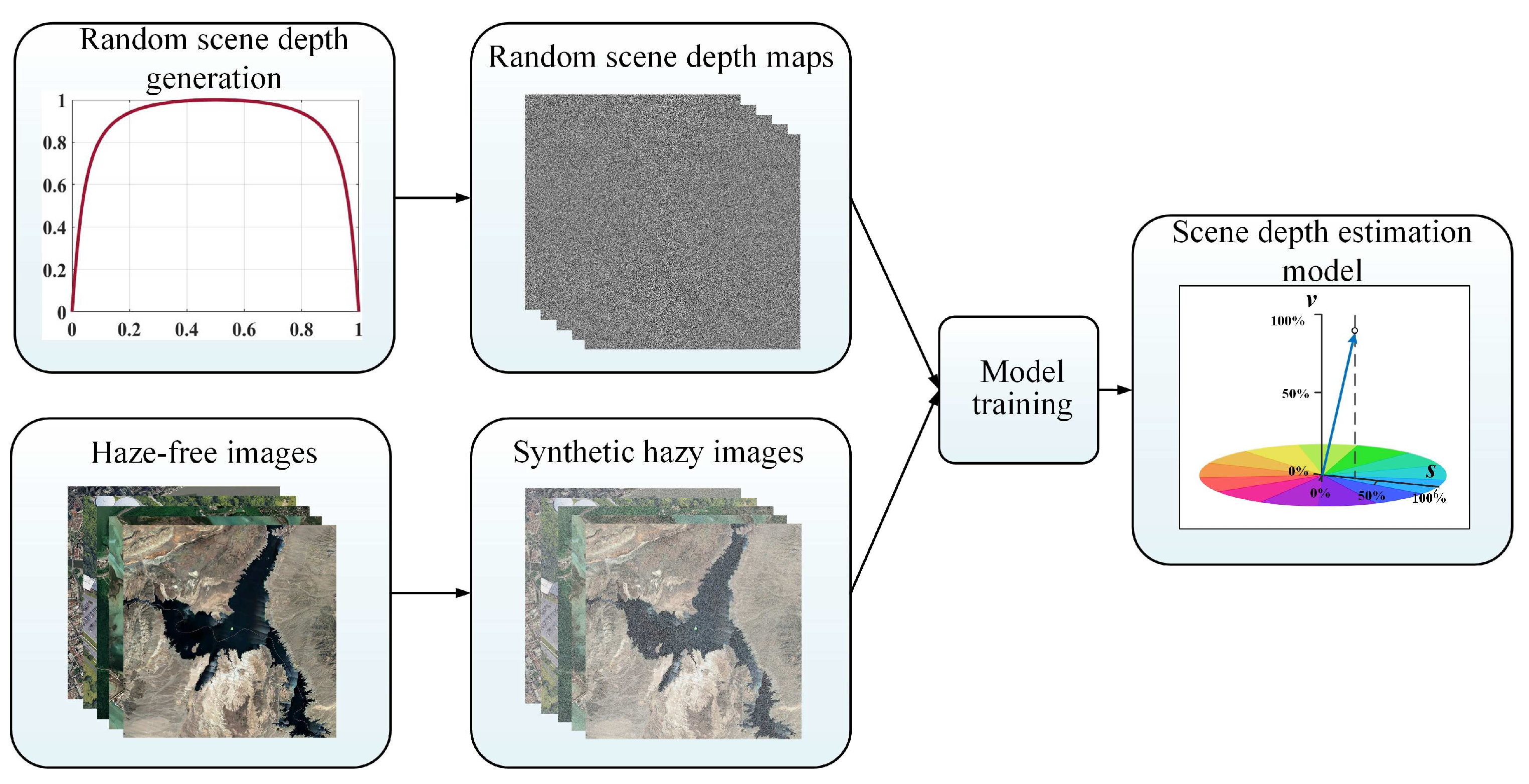
Due to haze or fog appearing in local regions, partial sections of remote sensing images are hazy. Different regions in a remote sensing image often have different fog densities. Figure 3b,c show different hazy regions of Figure 3a. The differences between brightness and saturation vary [6]. The hazy effect is correlated with these differences. Figure 3d illustrates the difference between brightness and saturation at each pixel point. This section presents the scene depth map estimation process of remote sensing images. Figure 4 shows the training process of a linear scene depth model for remote sensing images. A differentiable function is proposed to generate the scene depth of remote sensing images. Haze-free remote sensing images and generated scene depth maps are used to generate synthetic hazy images. Haze-free images and synthetic hazy images are used as training samples to train a scene depth estimation model. Sample images are trained by a gradient descent algorithm to obtain the linear parameters of the scene depth estimation model. After obtaining the trained parameters, an estimated scene depth map can be generated by the linear model of the original image.
3.1.1. The Definition of the Linear Model
Considering solid and liquid particles suspended in the atmosphere, aerosol directly causes the decrease of visibility in hazy weather conditions. The degraded images are often brighter and the color of scenery objects fades to varying degrees. The aerosol concentration is measured by aerosol optical depth (AOD) [34,35]. It is necessary to measure haze concentration for the parameter estimation. The extinction coefficient and AOD are often used to estimate haze concentration. However, this paper uses scene depth to measure haze concentration. All the images used in this paper were captured from the same satellite so that the extinction coefficient at the same height is relatively consistent [33]. The brightness of pixels in a hazy image is much higher than the one in a haze-free scene, and the saturation of these pixels is low [6]. Since haze concentration increases along with the change of the scene depth in general, this paper assumes that scene depth is proportional to haze concentration as follows.
where is the position within an image, d is the scene depth, c is the haze concentration, v is the scene brightness, and s is the saturation. The image is transformed to HSV-channel first. Then both scene brightness and saturation are calculated for each pixel . Finally, can be obtained. Therefore, a linear model can be defined as follows.
where , , are the unknown linear coefficients, is a random variable representing the random error of the model, and can be regarded as a random image.
When , , and are obtained by maximum likelihood estimation, the optimal solutions can be obtained. According to the continuously differentiable property of the distribution function, Equation (4) is obtained.
As given in Equation (3), the gradient of d can be calculated as follows:
where the constant term disappears in Equation (5). Since v and s are actually two single-channel images (the value and saturation channels of HSV spaces) from the divided hazy image I, Equation (5) ensures that d has an edge only if I has an edge. According to the above discussion, the scene depth information can be recovered by a linear model. In short, the edge-preserving property is the most important advantage of a linear model.
3.1.2. Training Data Collection
It is necessary to learn the coefficients , , and using the training data accurately. In this paper, the training samples consist of hazy remote sensing images and their corresponding ground truth scene depth maps. Unfortunately, there is no reliable way to measure the scene depth in a remote sensing image [6]. To obtain enough training samples, both haze-free remote sensing images and generated scene depth maps are used to compose corresponding hazy images for model training. A new continuously differentiable function F expressed as follows is proposed to generate random scene depth maps of remote sensing images.
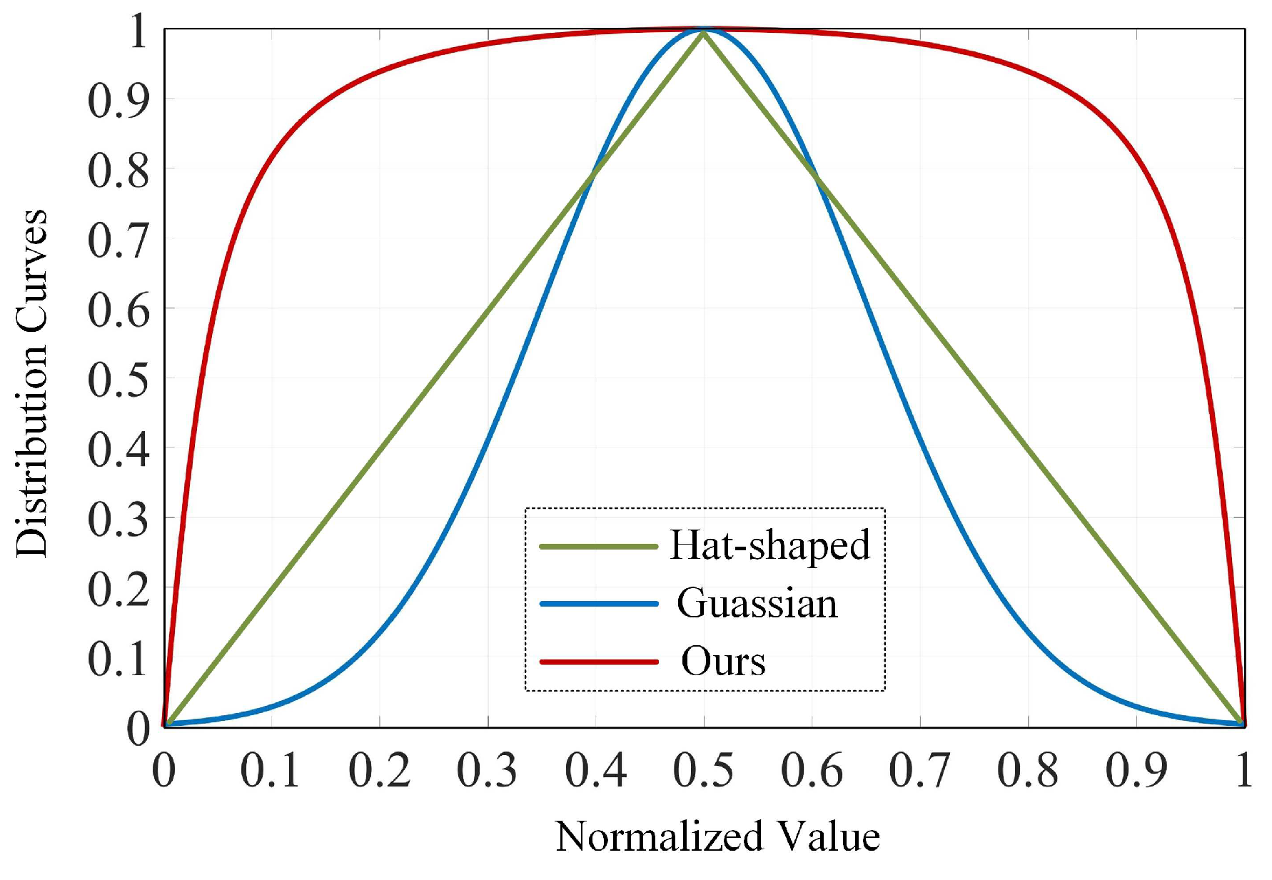
where k () is the pixel position, is the intensity value of the kth pixel, and is a fixed parameter. According to the comparison of the Gaussian [6], the hat shape of the curve, and the proposed functions shown in Figure 5, the proposed function curve has less penalty to small or big scene depth values and large distribution values in most cases, so it is suitable for scene depth map generation of remote sensing images.
For each haze-free remote sensing image, a random scene depth map d with the same size is generated. For the random atmospheric light , the value of is between 0.85 and 1.0 [31], which ensures that relatively real atmospheric light can be obtained. According to Equation (1), a synthetic hazy image with a random scene depth map d and random atmospheric A can be obtained. In this paper, 500 haze-free remote sensing images were used to generate the training samples (500 random scene depth maps and 500 synthetic hazy images) by supervised learning. The corresponding pre-existing labels were marked on all haze-free remote sensing images before the training process.
3.1.3. Learning Strategy
As the random error can be considered as independent, Equation (7) can be rewritten as follows.
where n is the total number of pixels within the training hazy images, is the scene depth of the nth pixel point, is the probability of , and L is the likelihood. If the random error at each pixel point is independent, Equation (7) can be rewritten as follows.
On the basis of Equations (4) and (8), Equation (9) can be obtained as follows.
where denotes the ground truth scene depth of the ith pixel point, and represent the brightness and saturation of the ith scene point, respectively. So, the problem is converted from the optimal values of , , and to the maximum L. It is difficult to find the appropriate values by maximizing L. L is the likelihood of the scene depth d. To obtain more scene depth information, L must be maximized to find the optimal parameters; however, it is difficult to directly maximize L to find the appropriate values, so is maximized to obtain the optimal parameters.
For the linear coefficients , , and , the gradient descent algorithm can be used to estimate the values. According to Equation (10), Equations (11)–(13) are obtained by taking the partial derivatives of with respect to , , and .
where , , and . To update the linear coefficients, the above expressions can be concisely expressed as follows, and the corresponding results can be obtained by iterations.
where is the learning rate, and the notation ⇐ represents the assignment of the value of the right side to on the left side. Equation (14) is used for dynamic iteration.
This paper uses the above-mentioned learning strategy to train the linear model. Both random scene depth maps and synthetic hazy images generated from 500 haze-free remote sensing images were used as training samples. A parameter controls the shape of function curve. When is small, the function curve is compressed. When is too large, the curve does not change much. To maintain the brightness of remote sensing images, the fixed parameter is set to a heuristic value 25. There are 1000 epochs in the proposed method, and the learning rate changes from to in different epochs. The initial parameters , , and are set to 0, 1, and −1, respectively. The optimal parameters obtained by learning the linear model are , , and . The random image can be generated by the proposed function. According to these parameters, the scene depths of hazy remote sensing images can be restored by Equation (3).
3.1.4. Scene Depth Restoration
According to the established relationship among the scene depth d, brightness v, saturation s, and estimated coefficients, a scene depth map of the given input image can be obtained by Equation (3). Unfortunately, the misclassification results in an inaccurate scene depth estimation in some cases. To overcome this issue, the neighboring pixels are considered. Under the assumption of local constancy in the scene depth, the raw scene depth map is processed as illustrated in Equation (15).
where is a neighborhood centered at , and is the scene depth map with the scale . According to the discussion of [6], the scale is set to 15 for noise reduction in the proposed method.
In this way, the restored scene depth map d can be applied to the estimation of the atmospheric light A.
3.2. Atmospheric Light Estimation
Atmospheric light estimation is achieved by position estimation. If d as the scene depth tends to infinity, t as the transmission map of the medium approaches zero [6]. Given a threshold , it is the smallest d in the top brightness pixels of the scene depth map. When , is treated as ∞. In most cases, hazy remote sensing images have the most distant views from the observer. In other words, the pixels farther away from the observer should have a large scene depth . Assuming the existence of distant views in each hazy image, Equation (16) is obtained.
where is the furthest pixel in a hazy image, is the maximum scene depth, y is a random pixel, and is the scene depth of pixel y. For each random pixel y, . Based on this assumption, the atmospheric light A can be obtained by as shown in Equation (17).
According to Equation (17), the top 0.1% of the brightest pixels in the scene depth map are chosen, and the pixel with the highest intensity in the corresponding hazy image I among these brightest pixels is selected as the atmospheric light A.
3.3. Transmission Map Estimation
In the previous section, the atmospheric light A is estimated. is transformed from the 3D RGB coordinate system to the spherical coordinate system with atmospheric light A as the spherical center. According to Equation (1), the is obtained. In spherical coordinates, has three dimensions , , and . r, , and are the distance to the origin (i.e., ), longitude, and latitude, respectively. For the given values of J and A, the only difference among scene points at different distances from the camera is the value of t. Hence, the change of t only affects , not and [7]. According to the closest sample point on the surface, the pixels are grouped based on their values.
For a given haze-line, depends on the objective distance, which can be calculated as follows.
When , corresponds to the largest radial coordinate. For a haze-line L that contains a haze-free pixel, the position of the haze-free pixel corresponds to the maximum radius . Figure 6 shows the distance distribution for each haze-line. For a remote sensing image, Figure 6a shows the layout of two different haze-lines in an image plane, and Figure 6b,c show the estimated radius distribution of the haze-lines marked in yellow and light blue, respectively. The haze-free pixel is assumed to exist in each haze line. The transmission based on the radius in each haze-line can be obtained. For all pixels, the initial transmission is estimated. So, the transmission map can be
obtained by the process of regularization [7].
3.4. Haze Removal
Haze removal is achieved by the atmospheric scattering model. Equation (1) holds for the scene radiance, whereas most of the camera-processed images do not have a linear relationship with the radiance [36]; therefore, the dehazing process should be applied to a radiometrically corrected image to obtain the best result [37]. After obtaining the atmospheric light A and transmission map , the scene radiance in the proposed
method can be expressed by Equation (19).
where J is the expected haze-free remote sensing image.
Algorithm 1 shows the main steps of the proposed dehazing algorithm of remote sensing images.
| Algorithm 1 The Proposed Dehazing Algorithm for Remote Sensing Images |
| Input: haze-free remote sensing images, hazy remote sensing image Output: dehazed image , scene depth map , atmospheric light A, transmission map
|
4. Comparative Experiments and Analysis
4.1. Experiment Preparation
The performance of the proposed image dehazing algorithm on remote sensing images was tested by the following comparative experiments. Hazy Geography, a dataset obtained from Google Earth, was used for evaluation. The comparative experiments process 100 remote sensing images randomly selected from various hazy geographic scenes. These sample images involve cities, geographic features (e.g., mountains, rivers), businesses, residences, and other types of geographic scenes. In addition, they have different sizes. The maximum size is , and the minimum size is .
As shown in Table 1, eleven methods, DCP, GPR, AMP, DEFADE, WCD, RRO, MOF, CAP, HLM, DN, and Proposed, were compared in the dehazing experiments of remote sensing images. DN is a deep learning based method, and the others are traditional dehazing methods. All the dehazed images obtained by the eleven methods were generated using the corresponding official open source codes. All the experiments were programmed using MATLAB 2016a in the Windows 10 environment on an Intel i7-7700k CPU@ 4.20-GHz desktop with 16.00GB RAM. Since a single evaluation index lacks objectivity, four evaluation indexes are introduced for a comprehensive analysis. The structural similarity () [38] index evaluates the structural similarity between two images by comparing luminance, contrast, and structure. The tone mapped image quality () [39] index mainly evaluates both structure preservation and naturalness. The fog aware density evaluator () [40] quantifies the haze concentration of a dehazed result. The peak signal-to-noise ratio () [41] represents the ratio between the maximum possible power of a signal and the power of corrupting noise that affects the representation fidelity of the signal—it is usually expressed in terms of the logarithmic decibel scale. Higher values for the , , and indexes are better and lower values for the index are better.
4.2. Comparative Experiment
4.2.1. Comparative Experiment in Real Hazy Scenes
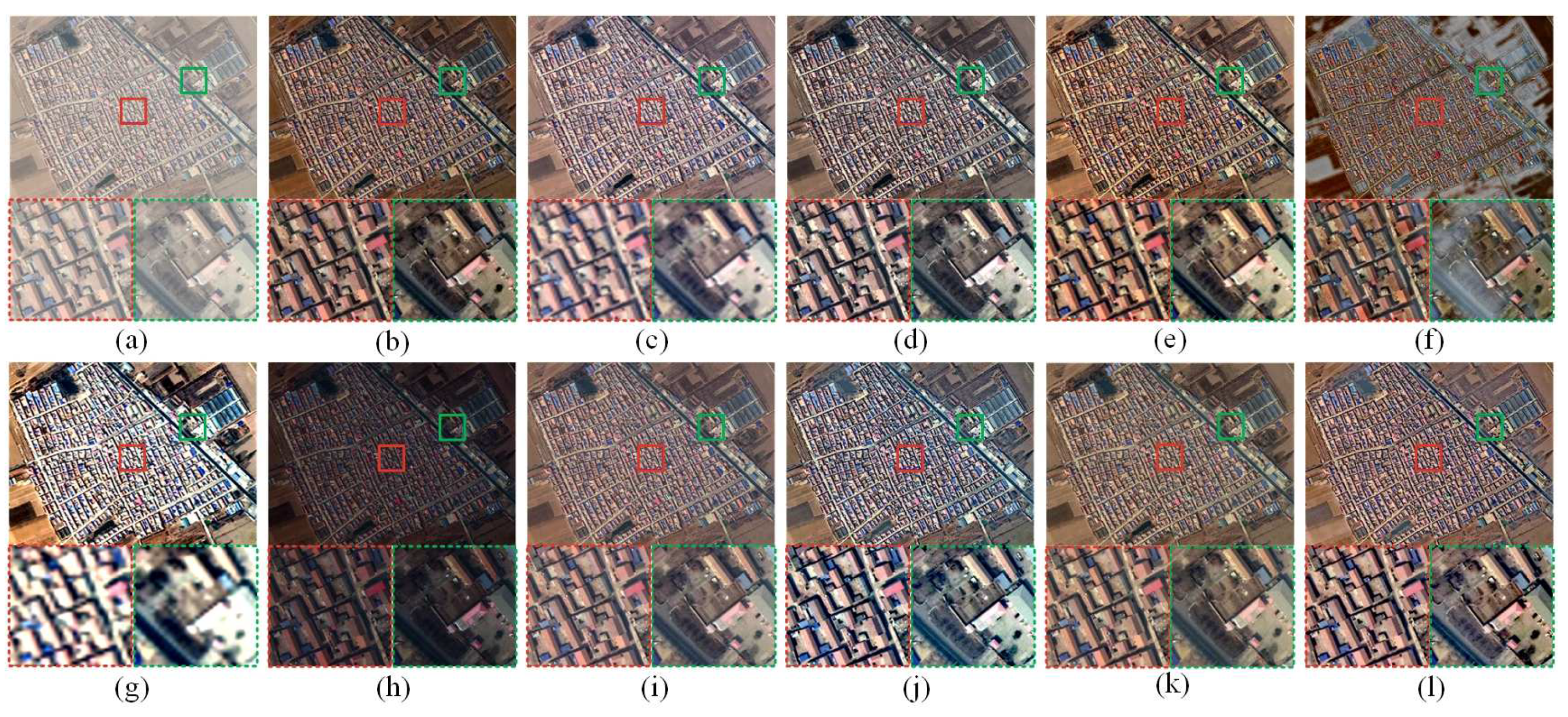
Figure 7 shows a dehazing example of a hazy remote sensing image. As shown in Figure 7b, the DCP method achieves a good dehazing effect, but the saturation of the dehazed image is high. The dehazed result obtained by the GPR method shown in Figure 7c is bright. According to Figure 7d,g,i, the dehazed images obtained by AMP, RRO, and HLM have poor performance in saturation. Furthermore, the detailed texture information of the original image is poorly preserved. The dehazed images of DEFADE method shown in Figure 7e has a poor visual effect due to the haze. As shown in Figure 7f, the dehazed image obtained by WCD method contains some white blocks. The dehazed image of MOF shown in Figure 7h has an unacceptable dark color tone. Compared with dehazed images shown in Figure 7i,k, the proposed image dehazing method has a better performance in dehazing effects, and achieves better visual effects in human perception.
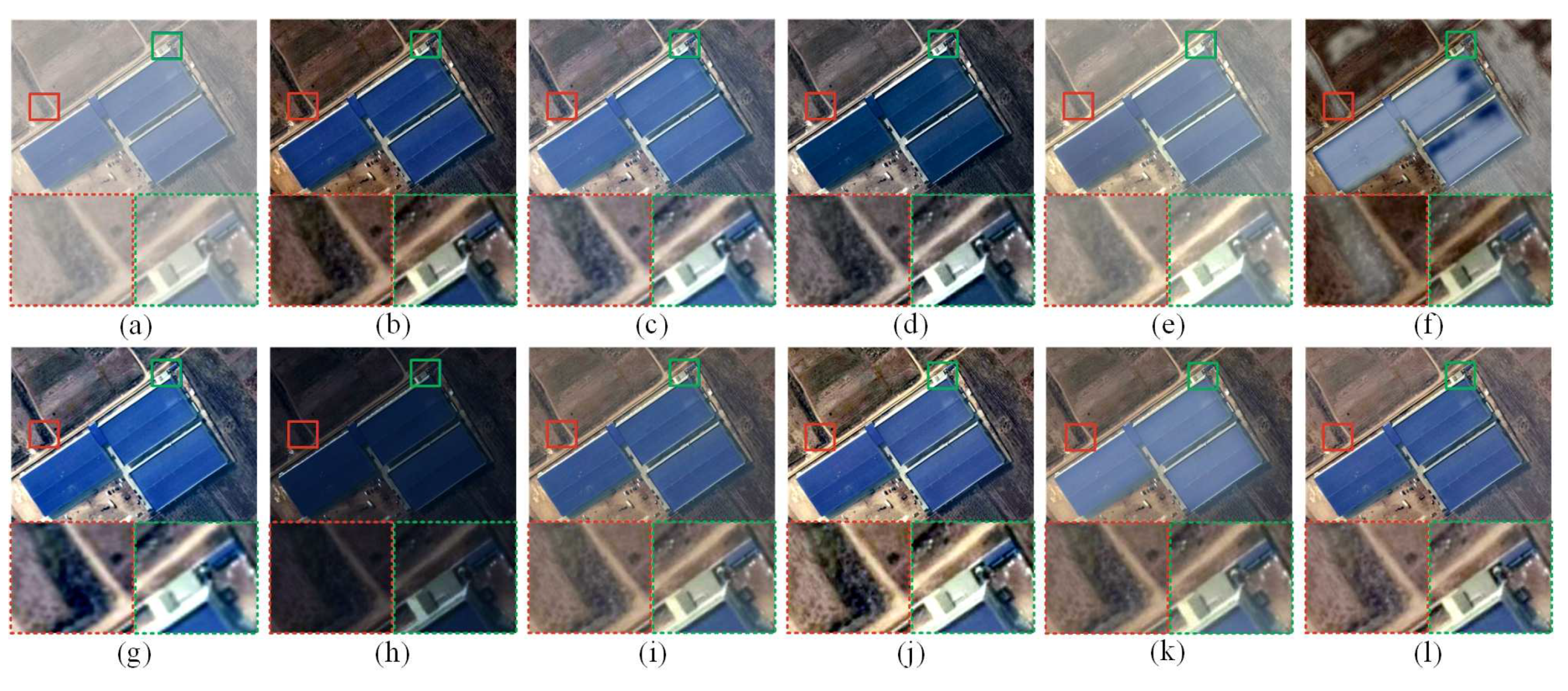
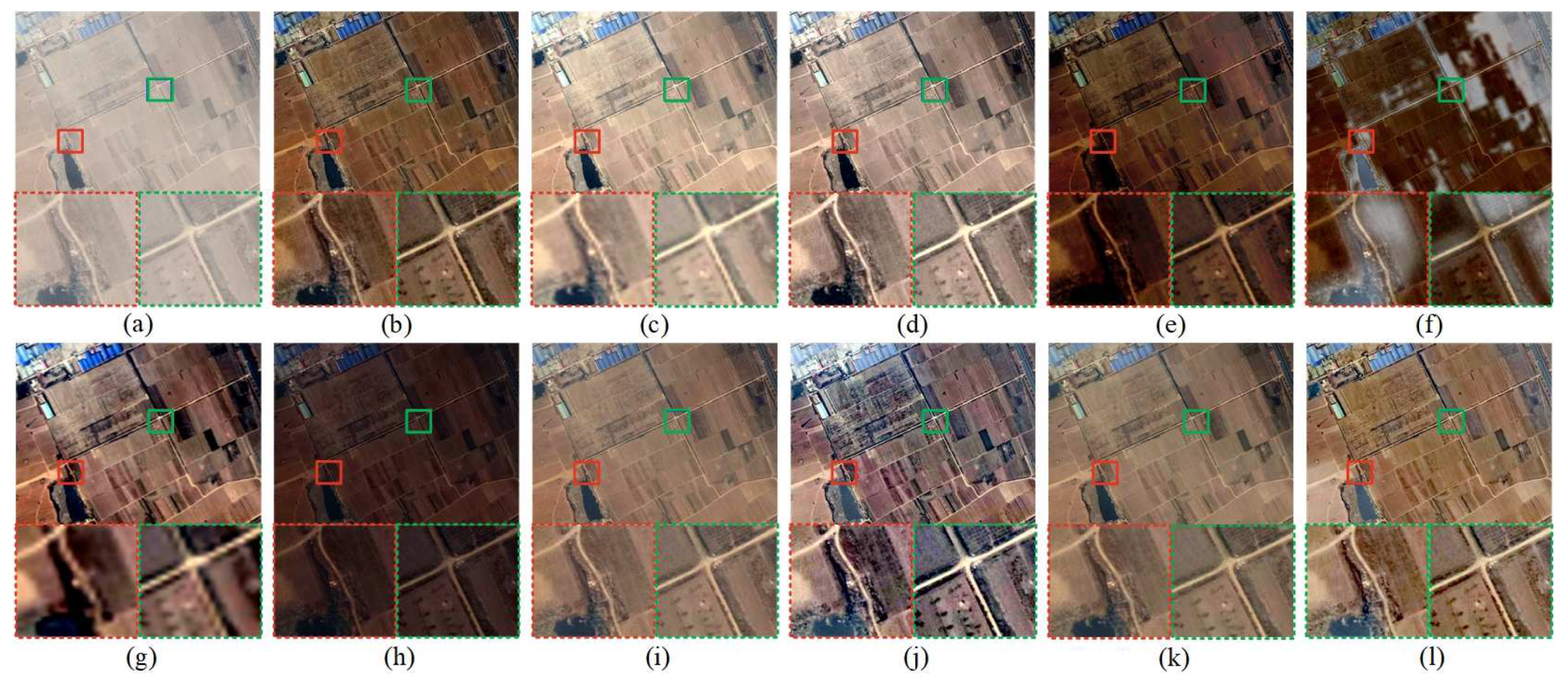
The experimental results of a hazy remote sensing image are presented in Figure 8. As shown in Figure 8b,k, the dehazed images obtained by DCP and DN have low brightness. The dehazed image of GPR in Figure 8c is bright but has a poor visual effect due to the haze. The saturation at the top-right corner in Figure 8d,j obtained by AMP and HLM, respectively, is bad. As shown in Figure 8f, some areas are blurry, and the color is not consistent in the dehazed result obtained by WCD. Figure 8g obtained by RRO is over-exposed with high saturation and contrast. The colors in Figure 8h obtained by MOF have poor visual effect due to darkness. As shown in Figure 8i, the haze is not completely removed in the dehazed result obtained by CAP, but CAP cannot effectively achieve the dehazing goal. Overall, compared with all other solutions, the dehazed image of the proposed method in Figure 8l has a better performance in visual effects.
Figure 9 shows the dehazing results of a remote sensing image. As shown in Figure 9b,e,h, the dehazed images obtained by DCP, DEFADE, and MOF are dark. Furthermore, the detailed texture information of the original image is poorly preserved. For the dehazed images obtained by GPR and AMP in Figure 9c,d, the image brightness is high, which retains less detailed texture information of image edges. The dehazed image obtained by MOF in Figure 9f has an unacceptable white color tone. According to the dehazed results obtained by RRO and HLM shown in Figure 9g,j, the overall saturation of the dehazed images is poor, and the appearance is not similar to the original. Compared with dehazed images obtained by CAP and DN in Figure 9i,k, the dehazed result of the proposed method has better color quality and is clearer.
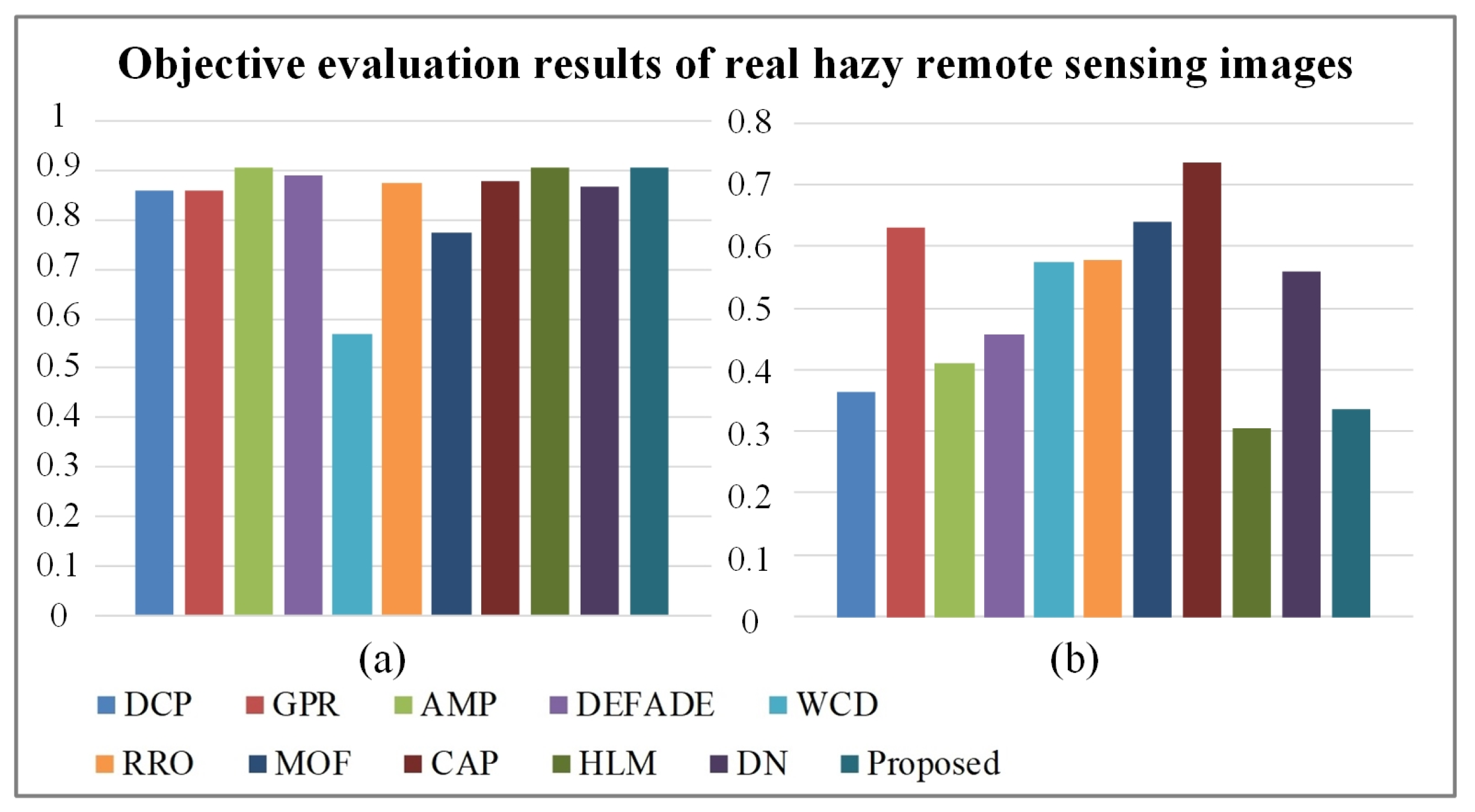
Two objective evaluation indexes and were used to evaluate the performance of eleven image dehazing methods in chrominance, dehazing effects, and so on. According to the objective evaluation results of image dehazing shown in Figure 10 and Table 2, the proposed method achieves a good overall performance among eleven image dehazing methods in real hazy scenes. DCP, AMP, HLM, and the proposed method achieve the top four ranks in , which means all of them can effectively remove image haze; however, DCP has the lowest value in , which means it has a poor performance in statistical naturalness. The proposed method has the highest score in , which means it has good performance in structure preservation and statistical naturalness. Overall the proposed method achieves good performance in and .
4.2.2. Comparative Experiment in Synthetic Hazy Scenes
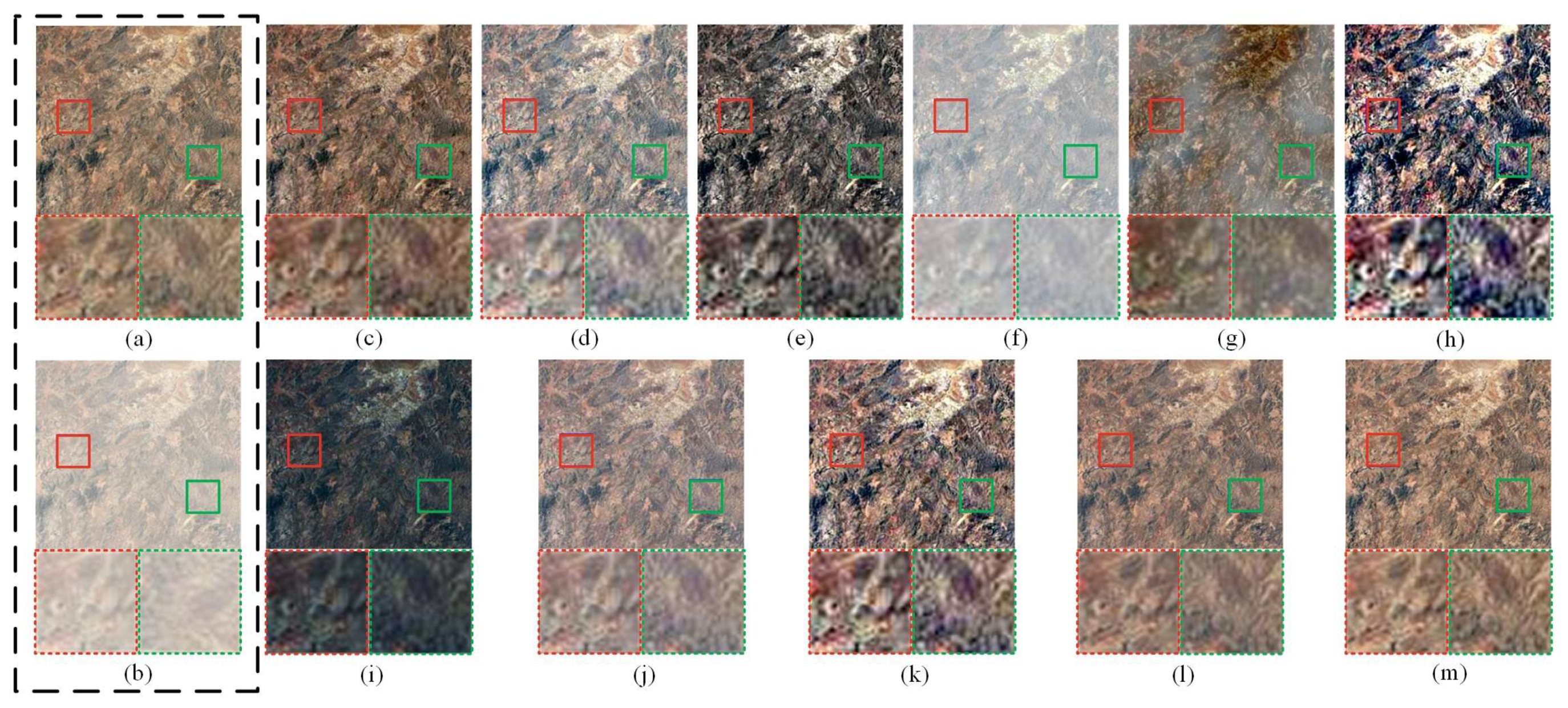
To verify the performance of the proposed method in similarity, noise, and color distortion, we designed a set of comparative experiments for haze removal of synthetic hazy remote sensing images. Figure 11 shows the dehazed results of a remote sensing image from a synthetic hazy scene. The results of AMP, RRO, MOF, and HL in Figure 11e,h,i,k show both relatively low brightness and color distortion. The results of GPR, DEFADE, WCD, and CAP shown in Figure 11d,f,g,j cannot effectively remove the haze from the synthetic hazy image. Compared with dehazed image obtained by DN in Figure 11l, the dehazed results of DCP and the proposed method have better dehazing performance.
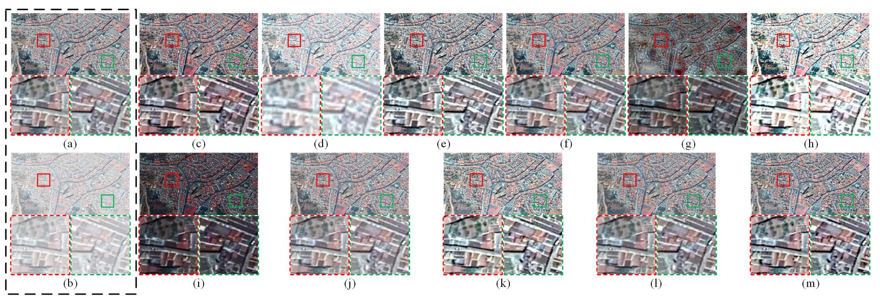
Figure 12 shows the dehazed results of a remote sensing urban image from a synthetic hazy scene. As shown in Figure 12g,i, the brightness of the dehazed images obtained by WCD and MOF is too low. The results of GPR and RRO in Figure 12d,h show both relatively high brightness and color distortion. Furthermore, GPR cannot effectively remove the haze from the synthetic hazy image. The overall saturation of the dehazed images obtained by DCP and DEFADE shown in Figure 12c,f is not similar to the original synthetic hazy image. As shown in Figure 12j,l, the detailed texture information of the edges of the dehazed images obtained by CAP and DN is not clear. Compared to the dehazed images obtained by AMP and HLM shown in Figure 12e,k, the dehazed result of the proposed method has higher color quality. So, the experimental results confirm that the proposed method can achieve good performance in remote sensing urban and non-urban scenes.
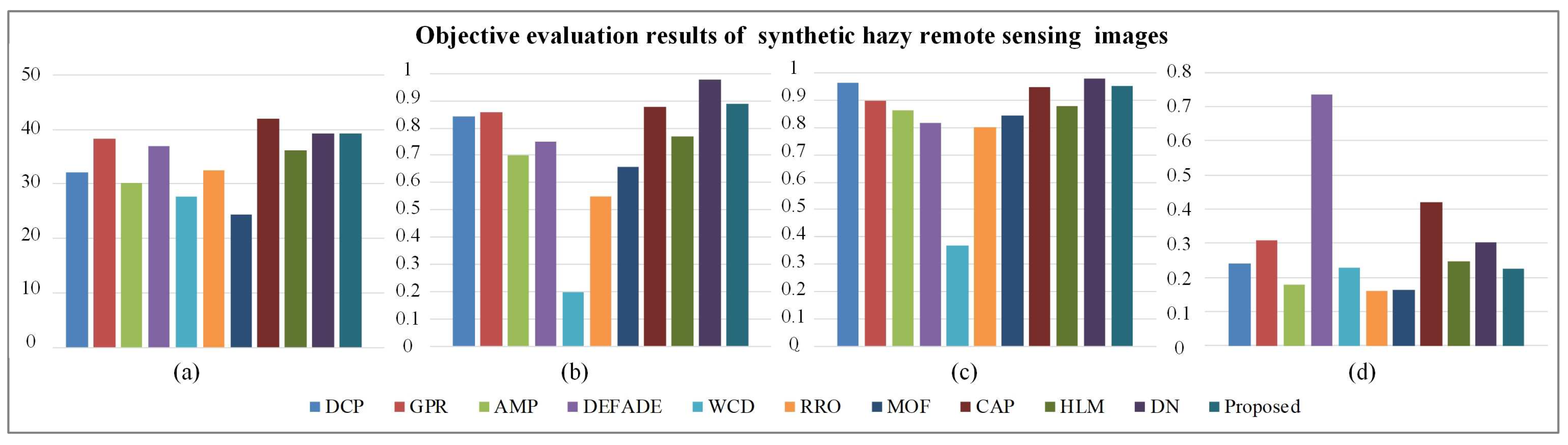
Table 3 and Figure 13 shows the results of four objective evaluation indexes for remote sensing images dehazing in synthetic hazy scenes. GPR, CAP, DN, and the proposed method have high scores, so the corresponding dehazed images obtained by them have high image quality. AMP, RRO, and MOF obtain high scores, but have low , , and scores. DN has the highest and scores, but its and scores are lower than the proposed method. In the comparative experiments, synthetic haze is added to haze-free remote sensing images. Significant differences in haze concentration exist between real hazy scenes and synthetic hazy scenes. The haze in remote sensing images from real hazy scenes is not completely uniform. The proposed method designs a depth training model for remote sensing images, which can remove the haze of remote sensing images from real scenes. For synthetic hazy images, the proposed method may not perform well; however, the experimental results in Table 3 show that the proposed method can still achieve the top four ranking in all four objective evaluation indexes, and effectively remove the haze from the synthetic image. DN, which is based on deep learning, directly trains an image as a model, which performs well in synthetic hazy scenes, but it does not have the same performance in real hazy scenes. The proposed method achieves good or comparable dehazing performance in all the metrics used to evaluate the dehazing performance of synthetic hazy images. Moreover, little color distortion is shown in the dehazed images obtained by the proposed method.
4.2.3. Comparison of Average Processing Time
As shown in Table 4, due to the high time complexity, the average processing time of the proposed solution is relatively long, about 14 times the fastest method (MOF). The proposed method first trains a linear scene depth model to obtain linear parameters, and then further estimates a scene depth map. Next, the obtained scene depth map is used to estimate the atmospheric light, and a haze-lines model is built to estimate the transmission map. Finally, the estimated atmospheric light and transmission map are input into the atmospheric scattering model to reconstruct the dehazed image. Note that the proposed method achieves good hazing performance on remote sensing images (shown in the previous two subsections).
5. Conclusions and Future Work
This paper proposed a novel atmospheric light estimation based dehazing framework for remote sensing images. According to color attenuation prior, a linear model was created to calculate the scene depth of the original image. A distribution function was proposed to generate a random scene depth map for a remote sensing image. The relationship between the original image and its corresponding scene depth map was built effectively by training the parameters of the linear model. The position of atmospheric light was estimated by means of the scene depth information. Then, a per-pixel transmission was estimated based on the haze-lines model. With the recovered transmission and atmospheric light, the dehazed remote sensing image can be easily removed by the atmospheric scattering model. The results of comparative experiments confirmed that the dehazing performance of the proposed method was good or comparable to both traditional and deep-learning based methods. Moreover, there was little color distortion in the dehazed images obtained by the proposed method. Due to the high time complexity, the average processing time of the proposed solution is relatively long. In future work, the proposed dehazing framework will be further optimized to reduce running time.
Author Contributions
Conceptualization, Z.Z., Y.L. (Yong Li), and G.Q.; methodology, Y.L. (Yong Li) and H.W.; software, Y.L. (Yaqin Luo) and H.W.; validation, Y.L. (Yaqin Luo), H.W., G.Q., Y.L. (Yong Li) and P.L.; formal analysis, Z.Z., Y.L. (Yaqin Luo), Y.L. (Yong Li), and Y.L. (Yuanyuan Li); investigation, Z.Z., Y.L. (Yaqin Luo), and Y.L. (Yong Li); resources, Y.L. (Yaqin Luo) and Y.L. (Yong Li); data curation, Y.L. (Yong Li) and H.W.; writing—original draft preparation, H.W. and G.Q.; writing—review and editing, Z.Z., G.Q., and N.M.; visualization, Y.L. (Yaqin Luo); supervision, Z.Z., Y.L. (Yuanyuan Li), and N.M.; project administration, Z.Z.; funding acquisition: Z.Z. and Y.L. (Yong Li). All authors have read and agreed to the published version of the manuscript.
Funding
This work is jointly supported by the National Natural Science Foundation of China under Grant Nos. 61803061, 61906026, and 61771081; Innovation research group of universities in Chongqing; the Chongqing Natural Science Foundation under Grant cstc2020jcyj-msxmX0577, and cstc2020jcyj-msxmX0634; “Chengdu-Chongqing Economic Circle” innovation funding of Chongqing Municipal Education Commission KJCXZD2020028; the Science and Technology Research Program of Chongqing Municipal Education Commission grants KJQN202000602; Ministry of Education China Mobile Research Fund (MCM 20180404); Special key project of Chongqing technology innovation and application development: cstc2019jscx-zdztzx0068.
Institutional Review Board Statement
Not applicable.
Informed Consent Statement
Not applicable.
Data Availability Statement
Not applicable.
Conflicts of Interest
The authors declare no conflict of interest.
References
- Yang, Y.; Newsam, S. Geographic image retrieval using local invariant features. IEEE Trans. Geosci. Remote Sens. 2012, 51, 818–832. [Google Scholar] [CrossRef]
- Liu, Q.; Gao, X.; He, L.; Lu, W. Haze removal for a single visible remote sensing image. Signal Process. 2017, 137, 33–43. [Google Scholar] [CrossRef]
- Xu, L.; Zhao, D.; Yan, Y.; Kwong, S.; Chen, J.; Duan, L.Y. IDeRs: Iterative dehazing method for single remote sensing image. Inf. Sci. 2019, 489, 50–62. [Google Scholar] [CrossRef]
- Zheng, M.; Qi, G.; Zhu, Z.; Li, Y.; Wei, H.; Liu, Y. Image Dehazing by An Artificial Image Fusion Method based on Adaptive Structure Decomposition. IEEE Sens. J. 2020, 20, 8062–8072. [Google Scholar] [CrossRef]
- Israël, H. Die Sichtweite im Nebel und die Möglichkeiten ihrer künstlichen Beeinflussung; Springer: Berlin/Heidelberg, Germany, 2013; Volume 640, pp. 33–55. [Google Scholar]
- Zhu, Q.; Mai, J.; Shao, L. A fast single image haze removal algorithm using color attenuation prior. IEEE Trans. Image Process. 2015, 24, 3522–3533. [Google Scholar] [PubMed] [Green Version]
- Berman, D.; Treibitz, T.; Avidan, S. Single Image Dehazing Using Haze-Lines. IEEE Trans. Pattern Anal. Mach. Intell. 2018, 42, 720–734. [Google Scholar] [CrossRef] [PubMed]
- Gao, Y.; Hu, H.M.; Wang, S.; Li, B. A fast image dehazing algorithm based on negative correction. Signal Process. 2014, 103, 380–398. [Google Scholar] [CrossRef]
- Thomas, G.; Flores-Tapia, D.; Pistorius, S. Histogram specification: A fast and flexible method to process digital images. IEEE Trans. Instrum. Meas. 2011, 60, 1565–1578. [Google Scholar] [CrossRef]
- Yu, L.; Liu, X.; Liu, G. A new dehazing algorithm based on overlapped sub-block homomorphic filtering. In Proceedings of the Eighth International Conference on Machine Vision, ICMV 2015, Barcelona, Spain, 19–20 November 2015. [Google Scholar]
- Li, Y.C.; Du, L.; Liu, S. Image Enhancement by Lift-Wavelet Based Homomorphic Filtering. In Proceedings of the International Conference on Electronics, Communications and Control, Xi’an, China, 23–25 August 2012; pp. 1623–1627. [Google Scholar]
- Qi, G.; Chang, L.; Luo, Y.; Chen, Y.; Zhu, Z.; Wang, S. A Precise Multi-Exposure Image Fusion Method Based on Low-level Features. Sensors 2020, 20, 1597. [Google Scholar] [CrossRef] [PubMed] [Green Version]
- Zhu, Z.; Wei, H.; Hu, G.; Li, Y.; Qi, G.; Mazur, N. A Novel Fast Single Image Dehazing Algorithm Based on Artificial Multiexposure Image Fusion. IEEE Trans. Instrum. Meas. 2021, 70, 1–23. [Google Scholar]
- Zhao, D.; Xu, L.; Yan, Y.; Chen, J.; Duan, L.Y. Multi-scale Optimal Fusion model for single image dehazing. Signal Process. Image Commun. 2019, 74, 253–265. [Google Scholar] [CrossRef]
- Zhu, Z.; Yin, H.; Chai, Y.; Li, Y.; Qi, G. A novel multi-modality image fusion method based on image decomposition and sparse representation. Inf. Sci. 2018, 432, 516–529. [Google Scholar] [CrossRef]
- Cai, B.; Xu, X.; Jia, K.; Qing, C.; Tao, D. Dehazenet: An end-to-end system for single image haze removal. IEEE Trans. Image Process. 2016, 25, 5187–5198. [Google Scholar] [CrossRef] [PubMed] [Green Version]
- Chiang, J.; Chen, Y. Underwater image enhancement by wavelength compensation and dehazing. IEEE Trans. Image Process. 2011, 21, 1756–1769. [Google Scholar] [CrossRef] [PubMed]
- Zhang, Y.; Guindon, B.; Cihlar, J. An image transform to characterize and compensate for spatial variations in thin cloud contamination of Landsat images. Remote Sens. Environ. 2002, 82, 173–187. [Google Scholar] [CrossRef]
- Chen, S.; Chen, X.; Chen, X.; Chen, J.; Cao, X.; Shen, M.; Yang, W.; Cui, X. A novel cloud removal method based on IHOT and the cloud trajectories for Landsat imagery. Remote Sens. 2018, 10, 1040. [Google Scholar] [CrossRef] [Green Version]
- Ni, W.; Gao, X.; Wang, Y. Single satellite image dehazing via linear intensity transformation and local property analysis. Neurocomputing 2016, 175, 25–39. [Google Scholar] [CrossRef]
- He, K.; Sun, J.; Tang, X. Single image haze removal using dark channel prior. IEEE Trans. Pattern Anal. Mach. Intell. 2010, 33, 2341–2353. [Google Scholar]
- Fan, X.; Wang, Y.; Tang, X.; Gao, R.; Luo, Z. Two-layer Gaussian process regression with example selection for image dehazing. IEEE Trans. Circuits Syst. Video Technol. 2016, 27, 2505–2517. [Google Scholar] [CrossRef]
- Singh, D.; Kumar, V. Image dehazing using Moore neighborhood-based gradient profile prior. Signal Process. Image Commun. 2019, 70, 131–144. [Google Scholar] [CrossRef]
- Zhu, M.; He, B.; Liu, J.; Yu, J. Boosting dark channel dehazing via weighted local constant assumption. Signal Process. 2020, 171, 107453. [Google Scholar] [CrossRef]
- Zhan, J.; Gao, Y.; Liu, X. Measuring the optical scattering characteristics of large particles in visible remote sensing. In Proceedings of the 2017 IEEE International Geoscience and Remote Sensing Symposium (IGARSS), Fort Worth, TX, USA, 23–28 July 2017; pp. 4666–4669. [Google Scholar]
- Wang, K.; Qi, G.; Zhu, Z.; Chai, Y. A Novel Geometric Dictionary Construction Approach for Sparse Representation Based Image Fusion. Entropy 2017, 19, 306. [Google Scholar] [CrossRef] [Green Version]
- Pan, X.; Xie, F.; Jiang, Z.; Yin, J. Haze removal for a single remote sensing image based on deformed haze imaging model. IEEE Signal Process. Lett. 2015, 22, 1806–1810. [Google Scholar] [CrossRef]
- Singh, D.; Kumar, V. Dehazing of remote sensing images using improved restoration model based dark channel prior. Imaging Sci. J. 2017, 65, 282–292. [Google Scholar] [CrossRef]
- Jiang, H.; Lu, N.; Yao, L.; Zhang, X. Single image dehazing for visible remote sensing based on tagged haze thickness maps. Remote Sens. Lett. 2018, 9, 627–635. [Google Scholar] [CrossRef]
- Bahat, Y.; Irani, M. Blind dehazing using internal patch recurrence. In Proceedings of the IEEE International Conference on Computational Photography (ICCP) 2016, Evanston, IL, USA, 13–15 May 2016; pp. 1–9. [Google Scholar]
- Tang, K.; Yang, J.; Wang, J. Investigating haze-relevant features in a learning framework for image dehazing. In Proceedings of the IEEE Conference on Computer Vision and Pattern Recognition, Columbus, OH, USA, 24–27 July 2014; pp. 2995–3000. [Google Scholar]
- Lee, S.; Yun, S.; Nam, J.H.; Won, C.S.; Jung, S.W. A review on dark channel prior based image dehazing algorithms. EURASIP J. Image Video Process. 2016, 2016, 4. [Google Scholar] [CrossRef] [Green Version]
- Sun, X.; Li, C.; Liu, L.; Yin, J.; Lei, Y.; Zhao, J. Dynamic Monitoring of Haze Pollution Using Satellite Remote Sensing. IEEE Sensors J. 2020, 20, 11802–11811. [Google Scholar] [CrossRef]
- Bilal, M.; Nichol, J.E.; Bleiweiss, M.P.; Dubois, D. A Simplified high resolution MODIS Aerosol Retrieval Algorithm (SARA) for use over mixed surfaces. Remote Sens. Environ. 2013, 136, 135–145. [Google Scholar] [CrossRef]
- Lolli, S.; Alparone, L.; Garzelli, A.; Vivone, G. Haze Correction for Contrast-Based Multispectral Pansharpening. IEEE Geosci. Remote Sens. Lett. 2017, 14, 2255–2259. [Google Scholar] [CrossRef]
- Chakrabarti, A.; Scharstein, D.; Zickler, T.E. An Empirical Camera Model for Internet Color Vision. In Proceedings of the BMVC, London, UK, 7–10 September 2009; Volume 1, p. 4. [Google Scholar]
- Lin, H.; Kim, S.J.; Süsstrunk, S.; Brown, M.S. Revisiting radiometric calibration for color computer vision. In Proceedings of the 2011 International Conference on Computer Vision, Barcelona, Spain, 6–13 November 2011; pp. 129–136. [Google Scholar]
- Wang, Z.; Bovik, A.; Sheikh, H.; Simoncelli, E. Image quality assessment: From error visibility to structural similarity. IEEE Trans. Image Process. 2004, 13, 600–612. [Google Scholar] [CrossRef] [PubMed] [Green Version]
- Yeganeh, H.; Wang, Z. Objective Quality Assessment of Tone-Mapped Images. IEEE Trans. Image Process. Publ. IEEE Signal Process. Soc. 2013, 22, 657–667. [Google Scholar] [CrossRef]
- Choi, L.; You, J.; Bovik, A. Referenceless prediction of perceptual fog density and perceptual image defogging. IEEE Trans. Image Process. 2015, 24, 3888–3901. [Google Scholar] [CrossRef]
- Hore, A.; Ziou, D. Image quality metrics: PSNR vs. SSIM. In Proceedings of the International Conference on Pattern Recognition, Istanbul, Turkey, 23–26 August 2010; pp. 2366–2369. [Google Scholar]
- Salazar-Colores, S.; Cruz-Aceves, I.; Ramos-Arreguin, J.M. Single image dehazing using a multilayer perceptron. J. Electron. Imaging 2018, 27, 1–11. [Google Scholar] [CrossRef]
- Shin, J.; Kim, M.; Paik, J.; Lee, S. Radiance-Reflectance Combined Optimization and Structure-Guided l0-Norm for Single Image Dehazing. IEEE Trans. Multimed. 2019, 22, 30–44. [Google Scholar] [CrossRef]
Figure 1.
A remote sensing image dehazing example; (a) a haze-free image; (b) a synthetic hazy image; (c) a dehazed synthetic image obtained by a haze-lines-based method [7]; (d) a dehazed synthetic image obtained by the proposed method.
Figure 1.
A remote sensing image dehazing example; (a) a haze-free image; (b) a synthetic hazy image; (c) a dehazed synthetic image obtained by a haze-lines-based method [7]; (d) a dehazed synthetic image obtained by the proposed method.

Figure 2.
The proposed dehazing framework for remote sensing images.
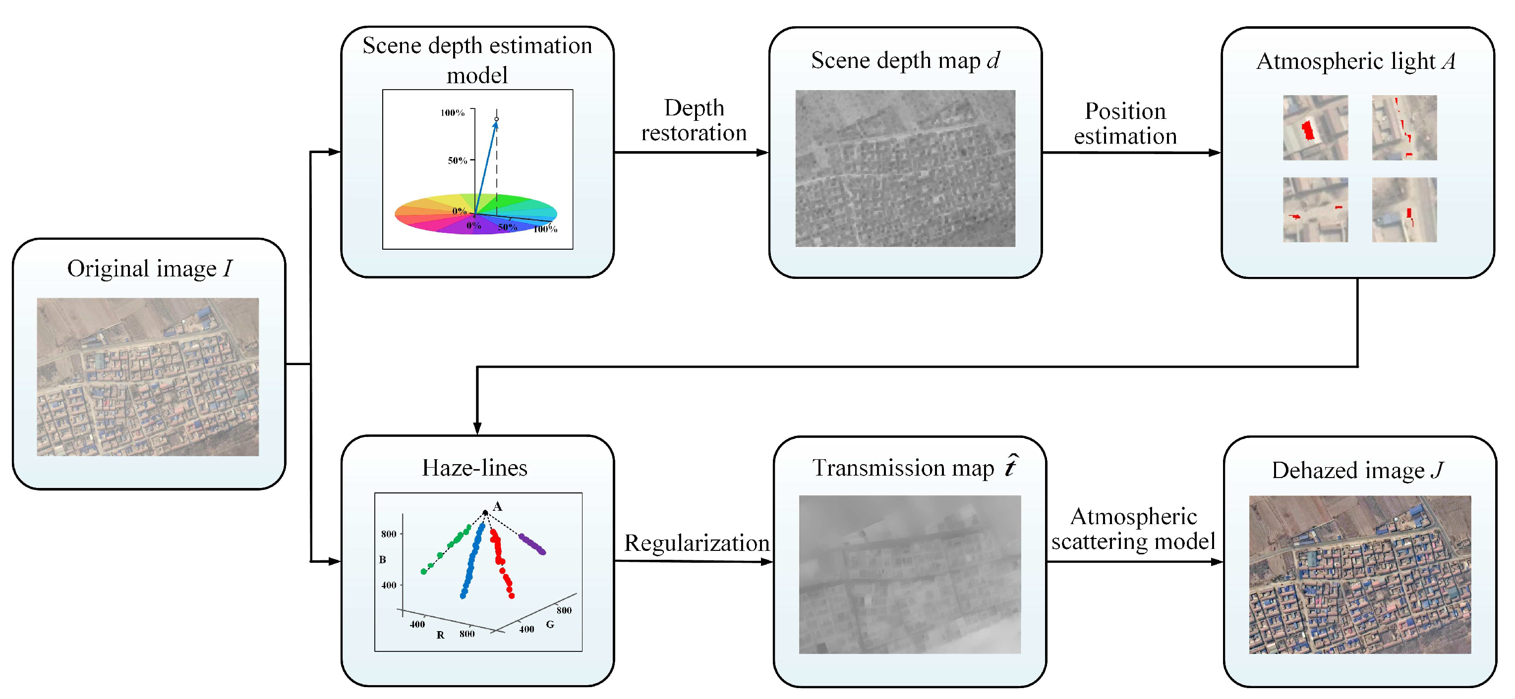
Figure 3.
The color attenuation of a hazy remote sensing image. (a) A hazy remote sensing image; (b,c) the partially enlarged images and the corresponding bar charts; (d) the difference between brightness and saturation.
Figure 3.
The color attenuation of a hazy remote sensing image. (a) A hazy remote sensing image; (b,c) the partially enlarged images and the corresponding bar charts; (d) the difference between brightness and saturation.

Figure 4.
The training process of a linear scene depth model for remote sensing images.

Figure 5.
Comparison of three different distribution functions.

Figure 6.
Distance distribution per haze-line of a sample image. (a) Pixels belonging to two different haze-lines are depicted in yellow and light blue, respectively. (b,c) A histogram of within each cluster for yellow and light blue haze-lines, respectively. The horizontal axis is limited to the range , as no pixel can be out of the radius range in this sample image.

Figure 7.
Dehazing example 1 of a remote sensing image from a real hazy scene: (a) Original; (b) DCP; (c) GPR; (d) AMP; (e) DEFADE; (f) WCD; (g) RRO; (h) MOF; (i) CAP; (j) HLM; (k) DN; (l) Proposed. Two partially enlarged images marked in red and green dotted frames correspond to the regions surrounded by red and green frames in the dehazed image.

Figure 8.
Dehazing example 2 of a remote sensing image from a real hazy scene: (a) Original; (b) DCP; (c) GPR; (d) AMP; (e) DEFADE; (f) WCD; (g) RRO; (h) MOF; (i) CAP; (j) HLM; (k) DN; (l) Proposed. Two partially enlarged images marked in red and green dotted frames correspond to the regions surrounded by red and green frames in the dehazed image.

Figure 9.
Dehazing example 3 of a remote sensing image from a real hazy scene: (a) Original; (b) DCP; (c) GPR; (d) AMP; (e) DEFADE; (f) WCD; (g) RRO; (h) MOF; (i) CAP; (j) HLM; (k) DN; (l) Proposed. Two partially enlarged images marked in red and green dotted frames correspond to the regions surrounded by red and green frames in the dehazed image.

Figure 10.
Objective evaluation results of eleven image dehazing methods in real hazy scenes: (a); (b) . The higher value of the index is better, the lower value of the FADE index is better.
Figure 10.
Objective evaluation results of eleven image dehazing methods in real hazy scenes: (a); (b) . The higher value of the index is better, the lower value of the FADE index is better.

Figure 11.
An image dehazing example of a remote sensing non-urban image from a synthetic hazy scene: (a) A haze-free image; (b) a synthetic hazy image; (c) DCP; (d) GPR; (e) AMP; (f) DEFADE; (g) WCD; (h) RRO; (i) MOF; (j) CAP; (k) HLM; (l) DN; (m) Proposed. Two partially enlarged images marked in red and green dotted frames correspond to the regions surrounded by red and green frames in the dehazed image.

Figure 12.
An image dehazing example of a remote sensing urban image from a synthetic hazy scene: (a) A haze-free image; (b) a synthetic hazy image; (c) DCP; (d) GPR; (e) AMP; (f) DEFADE; (g) WCD; (h) RRO; (i) MOF; (j) CAP; (k) HLM; (l) DN; (m) Proposed. Two partially enlarged images marked in red and green dotted frames correspond to the regions surrounded by red and green frames in the dehazed image.

Figure 13.
Objective evaluation results of eleven image dehazing methods in synthetic hazy scenes: (a) ; (b) ; (c); (d) . The higher values of the , , and indexes are better, the lower value of the FADE index is better.
Figure 13.
Objective evaluation results of eleven image dehazing methods in synthetic hazy scenes: (a) ; (b) ; (c); (d) . The higher values of the , , and indexes are better, the lower value of the FADE index is better.

Table 1.
Eleven remote sensing image dehazing methods for comparison.
| Short Explanation | |
|---|---|
| DCP | Dark Channel Prior [21] |
| GPR | Gaussian Process Regression [22] |
| AMP | A Multi-Layer Perceptron [42] |
| DEFADE | DEnsity of Fog Assessment based DEfogger [40] |
| WCD | Wavelength Compensation and Dehazing [17] |
| RRO | Radiance-Reflectance Combined Optimization [43] |
| MOF | Multi-scale Optimal Fusion [14] |
| CAP | Color Attenuation Prior [6] |
| HLM | Haze-lines Model [7] |
| DN | DehazeNet [16] |
| Proposed | ———— |
Table 2.
Evaluation of three objective indexes in image dehazing experiments of real hazy scenes. The top four results are marked in bold, and the corresponding rank is shown in the parenthesis (1: the best result, 2–4: the 2nd, 3rd, and 4th best results). The higher values of the index is better, the lower value of the index is better.
| TMQI | FADE | |
|---|---|---|
| DCP | 0.8602 | 0.3646(3) |
| GPR | 0.8582 | 0.6290 |
| AMP | 0.9050(2) | 0.4110(4) |
| DEFADE | 0.8917(4) | 0.4560 |
| WCD | 0.5698 | 0.5757 |
| RRO | 0.8749 | 0.5774 |
| MOF | 0.7734 | 0.6401 |
| CAP | 0.8780 | 0.7366 |
| HLM | 0.9044(3) | 0.3042(1) |
| DN | 0.8654 | 0.5598 |
| Proposed | 0.9055(1) | 0.3348(2) |
Table 3.
Evaluation of four objective indexes in image dehazing experiments of synthetic hazy scenes. The top four results are marked in bold, and the corresponding rank is shown in the parenthesis (1: the best result, 2–4: the 2nd, 3rd, and 4th best results). The higher values of the , and indexes are better, the lower value of the FADE index is better.
| PSNR | SSIM | TMQI | FADE | |
|---|---|---|---|---|
| DCP | 27.1712 | 0.8423 | 0.9659(2) | 0.2402 |
| GPR | 33.2397(4) | 0.8564(4) | 0.8982 | 0.3089 |
| AMP | 25.1680 | 0.6989 | 0.8646 | 0.1780(3) |
| DEFADE | 31.9961 | 0.7495 | 0.8180 | 0.7363 |
| WCD | 22.7210 | 0.1972 | 0.3690 | 0.2272 |
| RRO | 27.5368 | 0.5504 | 0.8009 | 0.1606(1) |
| MOF | 24.4369 | 0.6563 | 0.8442 | 0.1648(2) |
| CAP | 36.9671(1) | 0.8764(3) | 0.9469(4) | 0.4191 |
| HLM | 31.2391 | 0.7674 | 0.8786 | 0.2466 |
| DN | 34.2353(3) | 0.9786(1) | 0.9793(1) | 0.3032 |
| Proposed | 34.2522(2) | 0.8903(2) | 0.9519(3) | 0.2243(4) |
Table 4.
The average processing time of 100 hazy remote sensing images.
| DCP | GPR | AMP | DEFADE | WCD | RRO | MOF | CAP | HLM | DN | Proposed | |
|---|---|---|---|---|---|---|---|---|---|---|---|
| Time(s) | 9.3398 | 989.6070 | 4.3291 | 217.9994 | 16.9551 | 5.8158 | 1.4304 | 5.9325 | 25.7111 | 17.5564 | 19.9206 |
Publisher’s Note: MDPI stays neutral with regard to jurisdictional claims in published maps and institutional affiliations. |
© 2021 by the authors. Licensee MDPI, Basel, Switzerland. This article is an open access article distributed under the terms and conditions of the Creative Commons Attribution (CC BY) license (https://creativecommons.org/licenses/by/4.0/).
Share and Cite
MDPI and ACS Style
Zhu, Z.; Luo, Y.; Wei, H.; Li, Y.; Qi, G.; Mazur, N.; Li, Y.; Li, P. Atmospheric Light Estimation Based Remote Sensing Image Dehazing. Remote Sens. 2021, 13, 2432. https://0-doi-org.brum.beds.ac.uk/10.3390/rs13132432
AMA Style
Zhu Z, Luo Y, Wei H, Li Y, Qi G, Mazur N, Li Y, Li P. Atmospheric Light Estimation Based Remote Sensing Image Dehazing. Remote Sensing. 2021; 13(13):2432. https://0-doi-org.brum.beds.ac.uk/10.3390/rs13132432
Chicago/Turabian StyleZhu, Zhiqin, Yaqin Luo, Hongyan Wei, Yong Li, Guanqiu Qi, Neal Mazur, Yuanyuan Li, and Penglong Li. 2021. "Atmospheric Light Estimation Based Remote Sensing Image Dehazing" Remote Sensing 13, no. 13: 2432. https://0-doi-org.brum.beds.ac.uk/10.3390/rs13132432
Note that from the first issue of 2016, this journal uses article numbers instead of page numbers. See further details here.