
Using Machine Learning Methods to Identify Particle Types from Doppler Lidar Measurements in Iceland

 , , and
Abstract
:
1. Introduction
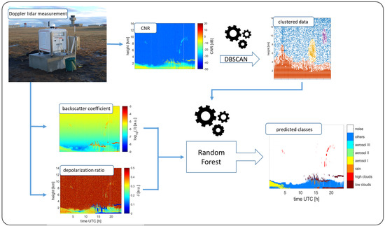
2. Methodology
2.1. Instrument and Data Description
2.2. Machine Learning Algorithms
- a.
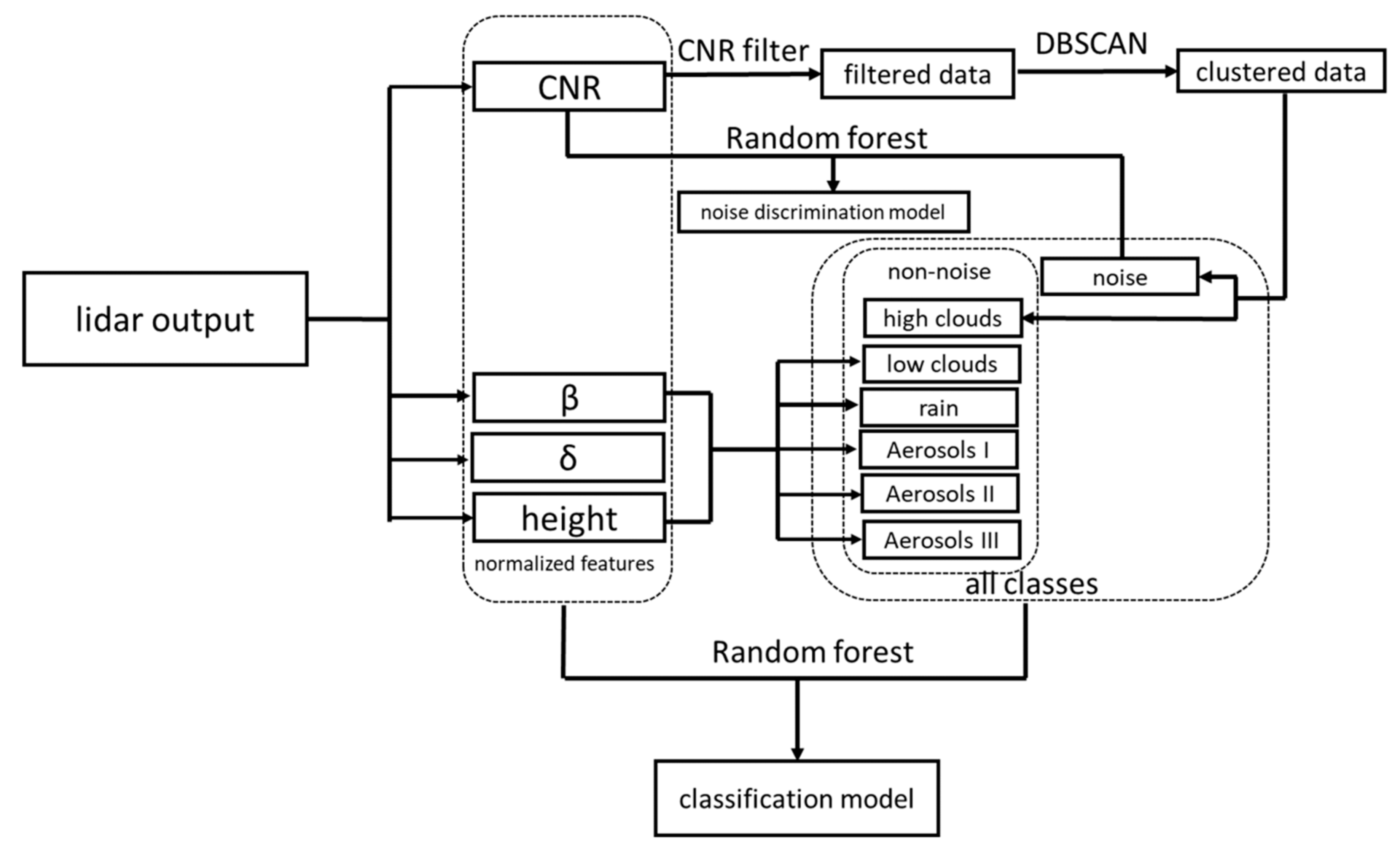
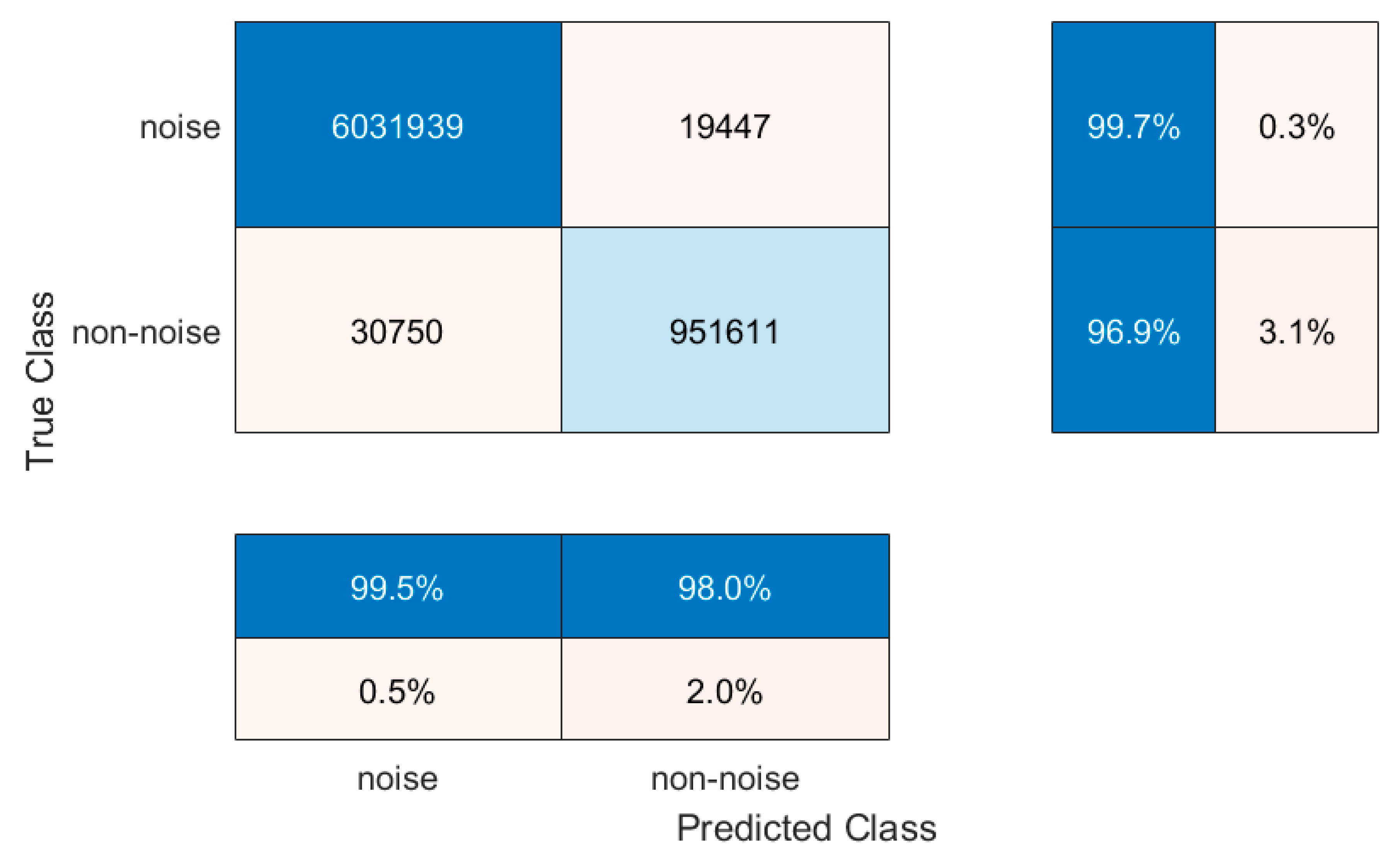
- Noise Discrimination Model
- b.
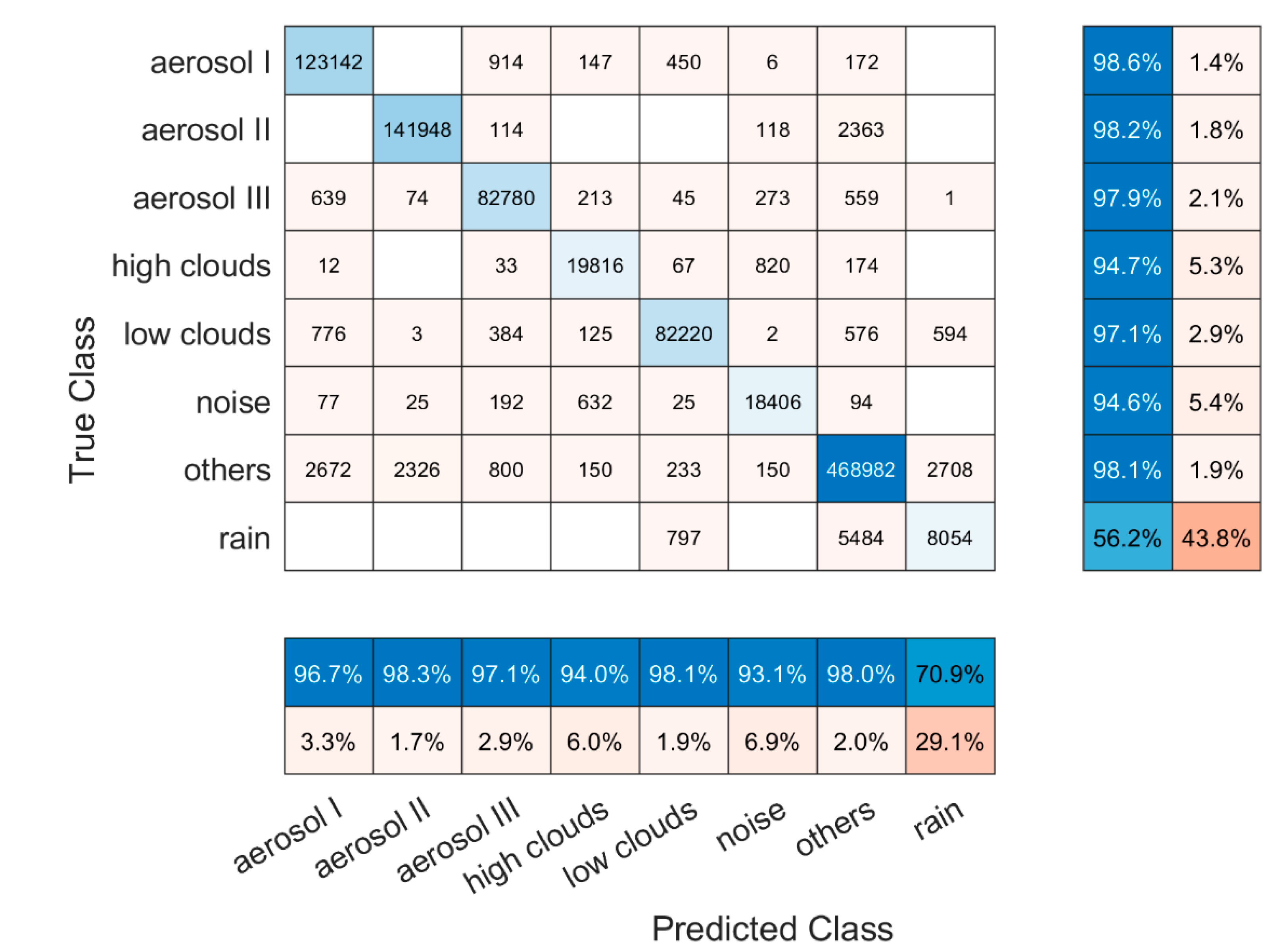
- Classification Model
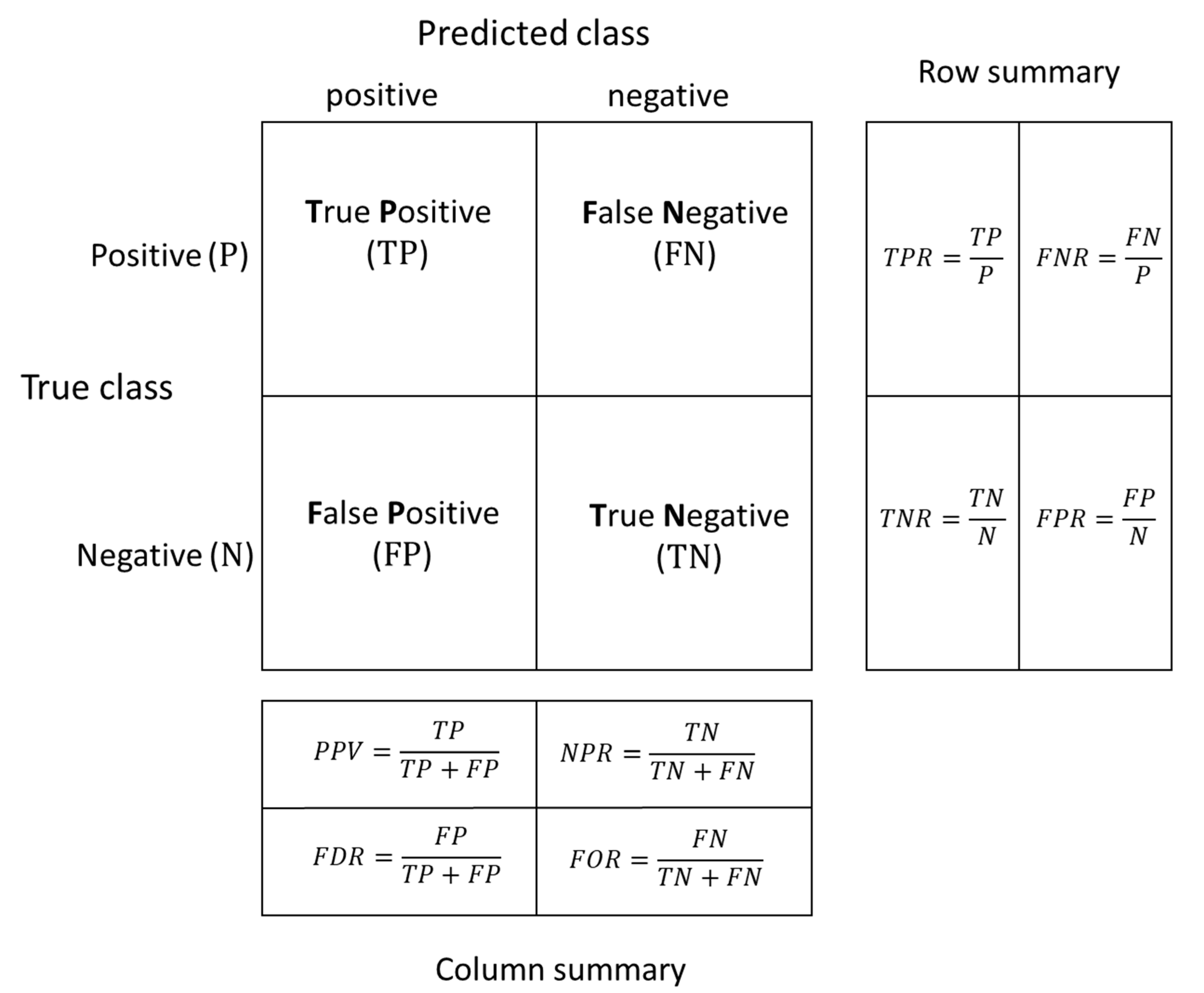
2.3. Model Performance Evaluation
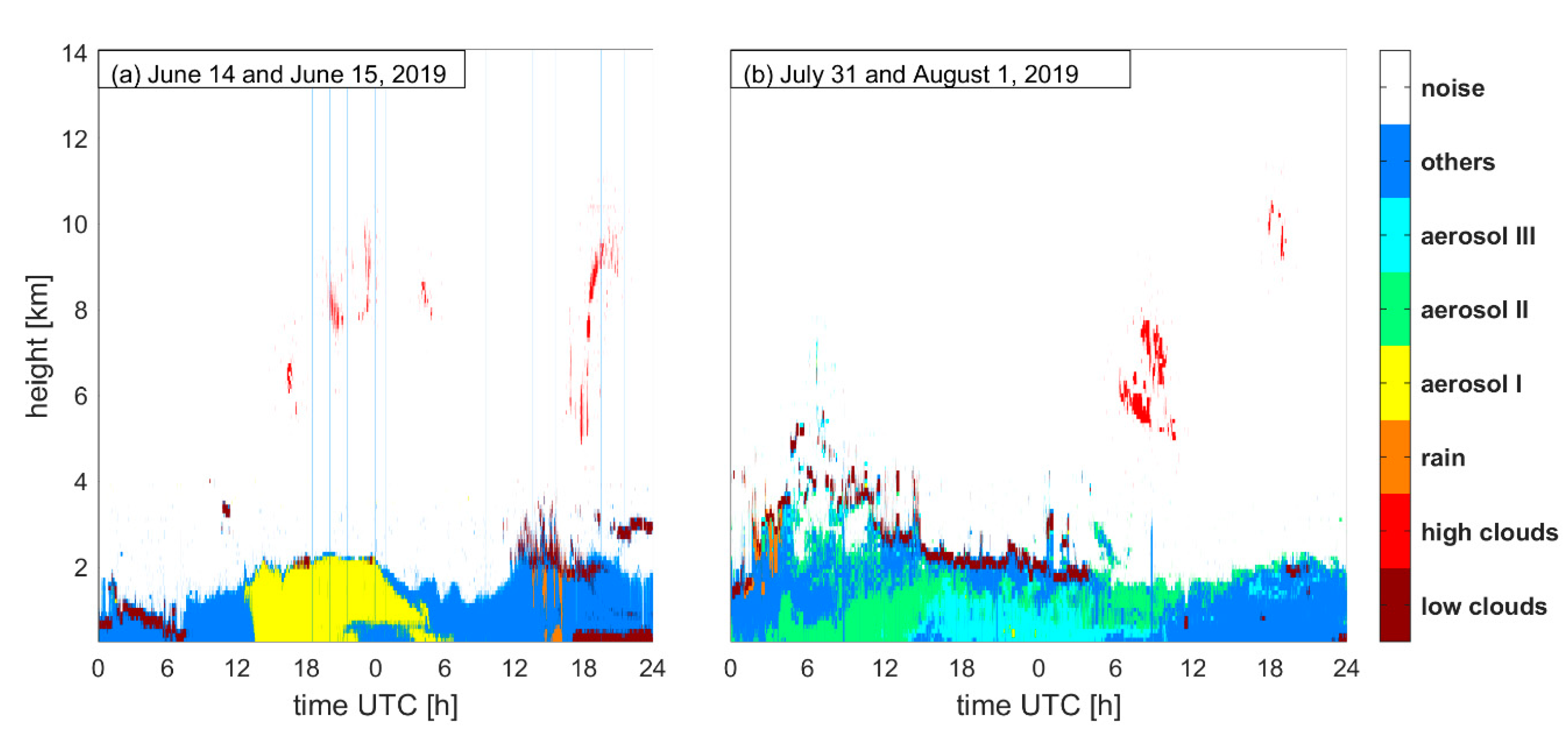
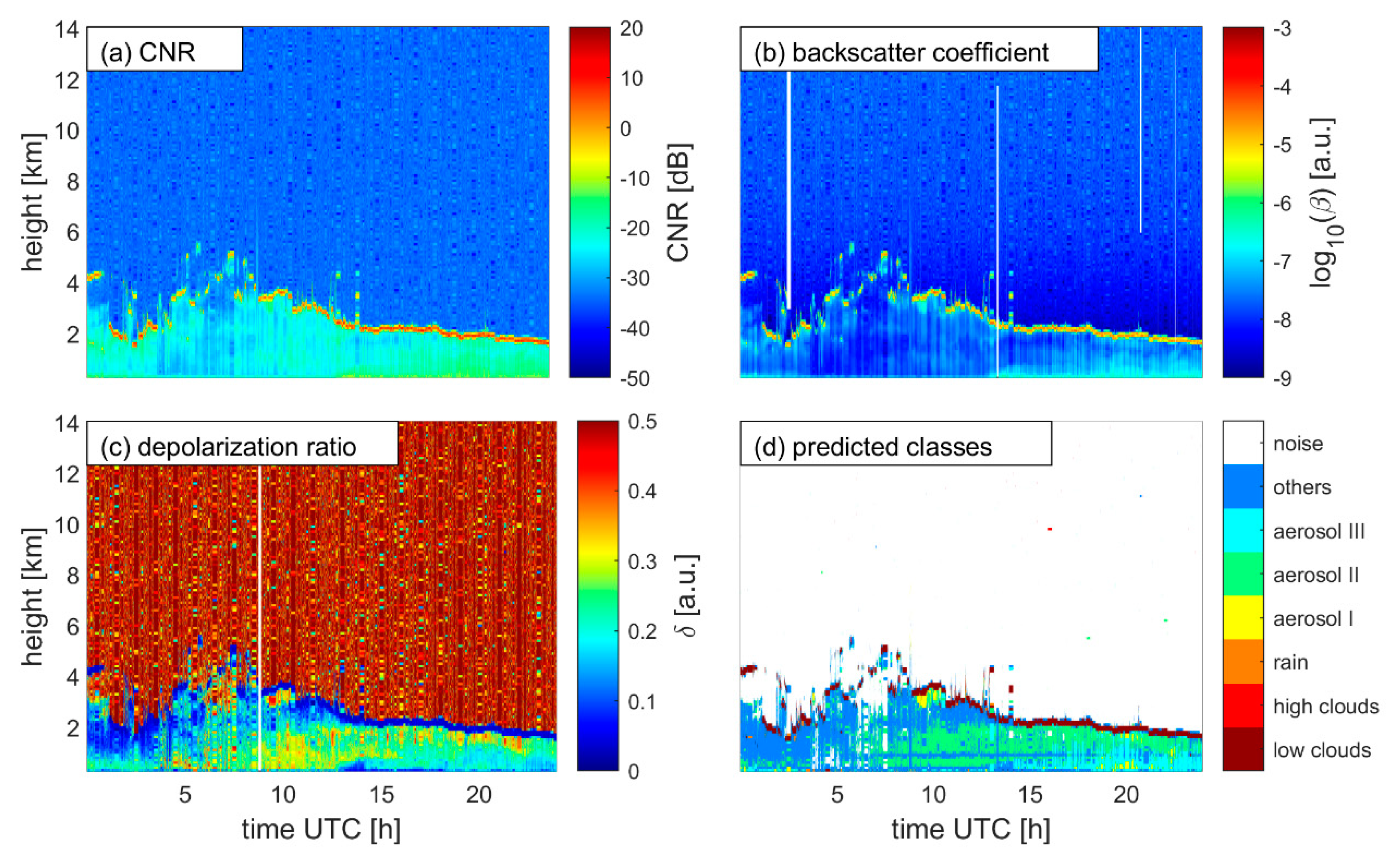
3. Results
4. Discussion and Suggestions
5. Conclusions
Author Contributions
Funding
Institutional Review Board Statement
Informed Consent Statement
Conflicts of Interest
References
- Gao, H.; Cheng, B.; Wang, J.; Li, K.; Zhao, J.; Li, D. Object Classification Using CNN-Based Fusion of Vision and LIDAR in Autonomous Vehicle Environment. IEEE Trans. Ind. Inform. 2018, 14, 4224–4231. [Google Scholar] [CrossRef]
- Dubayah, R.O.; Drake, J.B. Lidar Remote Sensing for Forestry. J. For. 2000, 98, 44–46. [Google Scholar] [CrossRef]
- Thobois, L.; Cariou, J.P.; Gultepe, I. Review of Lidar-Based Applications for Aviation Weather. Pure Appl. Geophys. 2019, 176, 1959–1976. [Google Scholar] [CrossRef]
- Yang, S.; Petersen, G.N.; von Löwis, S.; Preißler, J.; Finger, D.C. Determination of Eddy Dissipation Rate by Doppler Lidar in Reykjavik, Iceland. Meteorol. Appl. 2020, 27, e1951. [Google Scholar] [CrossRef]
- Bilbro, J.; Fichtl, G.; Fitzjarrald, D.; Krause, M.; Lee, R. Airborne Doppler Lidar Wind Field Measurements. Bull. Am. Meteorol. Soc. 1984, 65, 348–359. [Google Scholar] [CrossRef] [Green Version]
- Ansmann, A.; Müller, D. Lidar and Atmospheric Aerosol Particles. In Lidar: Range-Resolved Optical Remote Sensing of the Atmosphere; Weitkamp, C., Ed.; Springer Series in Optical Sciences; Springer: New York, NY, USA, 2005; pp. 105–141. ISBN 978-0-387-25101-1. [Google Scholar]
- Boquet, M.; Royer, P.; Cariou, J.-P.; Machta, M.; Valla, M. Simulation of Doppler Lidar Measurement Range and Data Availability. J. Atmos. Ocean. Technol. 2016, 33, 977–987. [Google Scholar] [CrossRef]
- Gryning, S.-E.; Floors, R.; Peña, A.; Batchvarova, E.; Brümmer, B. Weibull Wind-Speed Distribution Parameters Derived from a Combination of Wind-Lidar and Tall-Mast Measurements Over Land, Coastal and Marine Sites. Bound. Layer Meteorol. 2016, 159, 329–348. [Google Scholar] [CrossRef] [Green Version]
- Gryning, S.-E.; Mikkelsen, T.; Baehr, C.; Dabas, A.; Gómez, P.; O’Connor, E.; Rottner, L.; Sjöholm, M.; Suomi, I.; Vasiljević, N. Measurement methodologies for wind energy based on ground-level remote sensing. In Renewable Energy Forecasting; Elsevier: Sawston, Cambridge, 2017; pp. 29–56. ISBN 978-0-08-100504-0. [Google Scholar]
- Di Noia, A.; Hasekamp, O.P. Neural Networks and Support Vector Machines and Their Application to Aerosol and Cloud Remote Sensing: A Review. In Springer Series in Light Scattering: Volume 1: Multiple Light Scattering, Radiative Transfer and Remote Sensing; Kokhanovsky, A., Ed.; Springer Series in Light Scattering; Springer International Publishing: Cham, Germany, 2018; pp. 279–329. ISBN 978-3-319-70796-9. [Google Scholar]
- Groß, S.; Tesche, M.; Freudenthaler, V.; Toledano, C.; Wiegner, M.; Ansmann, A.; Althausen, D.; Seefeldner, M. Characterization of Saharan Dust, Marine Aerosols and Mixtures of Biomass-Burning Aerosols and Dust by Means of Multi-Wavelength Depolarization and Raman Lidar Measurements during SAMUM 2. Tellus B Chem. Phys. Meteorol. 2011, 63, 706–724. [Google Scholar] [CrossRef]
- Chouza, F.; Reitebuch, O.; Groß, S.; Rahm, S.; Freudenthaler, V.; Toledano, C.; Weinzierl, B. Retrieval of Aerosol Backscatter and Extinction from Airborne Coherent Doppler Wind Lidar Measurements. Atmos. Meas. Tech. 2015, 8, 2909–2926. [Google Scholar] [CrossRef] [Green Version]
- Haarig, M.; Ansmann, A.; Gasteiger, J.; Kandler, K.; Althausen, D.; Baars, H.; Radenz, M.; Farrell, D.A. Dry versus Wet Marine Particle Optical Properties: RH Dependence of Depolarization Ratio, Backscatter, and Extinction from Multiwavelength Lidar Measurements during SALTRACE. Atmos. Chem. Phys. 2017, 17, 14199–14217. [Google Scholar] [CrossRef] [Green Version]
- Leosphere, Inc. WINDCUBE 100s-200s User Manual Version 2; Leosphere Inc.: Orsay, France, 2013. [Google Scholar]
- Kotsiantis, S.B.; Zaharakis, I.D.; Pintelas, P.E. Machine Learning: A Review of Classification and Combining Techniques. Artif. Intell. Rev. 2006, 26, 159–190. [Google Scholar] [CrossRef]
- Zeng, S.; Vaughan, M.; Liu, Z.; Trepte, C.; Kar, J.; Omar, A.; Winker, D.; Lucker, P.; Hu, Y.; Getzewich, B.; et al. Application of High-Dimensional Fuzzy k-Means Cluster Analysis to CALIOP/CALIPSO Version 4.1 Cloud–Aerosol Discrimination. Atmos. Meas. Tech. 2019, 12, 2261–2285. [Google Scholar] [CrossRef] [Green Version]
- Brakhasi, F.; Hajeb, M.; Fouladinejad, F. Discrimination Aerosol Form Clouds Using Cats-Iss Lidar Observations Based on Random Forest and Svm Algorithms over The Eastern Part of Middle East. ISPRS Int. Arch. Photogramm. Remote Sens. Spat. Inf. Sci. 2019, XLII-4/W18, 235–240. [Google Scholar] [CrossRef] [Green Version]
- Farhani, G.; Sica, R.J.; Daley, M.J. Classification of Lidar Measurements Using Supervised and Unsupervised Machine Learning Methods. Atmos. Meas. Tech. Discuss. 2020, 1–18. [Google Scholar] [CrossRef]
- Maxwell, A.E.; Warner, T.A.; Fang, F. Implementation of Machine-Learning Classification in Remote Sensing: An Applied Review. Int. J. Remote Sens. 2018, 39, 2784–2817. [Google Scholar] [CrossRef] [Green Version]
- Yang, S.; Preißler, J.; Wiegner, M.; von Löwis, S.; Petersen, G.N.; Parks, M.M.; Finger, D.C. Monitoring Dust Events Using Doppler Lidar and Ceilometer in Iceland. Atmosphere 2020, 11, 1294. [Google Scholar] [CrossRef]
- Ólafsson, H.; Furger, M.; Brümmer, B. The Weather and Climate of Iceland. Meteorol. Z. 2007, 16, 5–8. [Google Scholar] [CrossRef]
- Breiman, L. Random Forests. Mach. Learn. 2001, 45, 5–32. [Google Scholar] [CrossRef] [Green Version]
- Belgiu, M.; Drăguţ, L. Random Forest in Remote Sensing: A Review of Applications and Future Directions. ISPRS J. Photogramm. Remote Sens. 2016, 114, 24–31. [Google Scholar] [CrossRef]
- Liu, B.; Xu, Z.; Kang, Y.; Cao, Y.; Pei, L. Air Pollution Lidar Signals Classification Based on Machine Learning Methods. In Proceedings of the 2020 39th Chinese Control Conference (CCC), Shenyang, China, 27–29 July 2020; pp. 13–18. [Google Scholar]
- Mellor, A.; Boukir, S.; Haywood, A.; Jones, S. Exploring Issues of Training Data Imbalance and Mislabelling on Random Forest Performance for Large Area Land Cover Classification Using the Ensemble Margin. ISPRS J. Photogramm. Remote Sens. 2015, 105, 155–168. [Google Scholar] [CrossRef]
- Ester, M.; Kriegel, H.-P.; Sander, J.; Xu, X. A Density-Based Algorithm for Discovering Clusters in Large Spatial Databases with Noise. In Proceedings of the Second International Conference on Knowledge Discovery and Data Mining, Portland, OR, USA, 2 August 1996; pp. 226–231. [Google Scholar]
- Schubert, E.; Sander, J.; Ester, M.; Kriegel, H.P.; Xu, X. DBSCAN Revisited, Revisited: Why and How You Should (Still) Use DBSCAN. ACM Trans. Database Syst. 2017, 42, 19:1–19:21. [Google Scholar] [CrossRef]
- Fawcett, T. An Introduction to ROC Analysis. Pattern Recognit. Lett. 2006, 27, 861–874. [Google Scholar] [CrossRef]


| Model | Windcube 200S |
|---|---|
| manufacturer | Leosphere Inc. |
| wavelength (μm) | 1.54 |
| detection range (m) | 50–14,000 |
| range resolution (m) | 25, 50, 75, 100 |
| elevation angle (°) | −10–90 |
| azimuth angle (°) | 0–360 |
| Group | Class Name | Labeling Method * | Physical Explanation |
|---|---|---|---|
| 1 | Low clouds | Highest backscatter coefficient; low depolarization ratio | Clouds within or close to the boundary layer; mostly water clouds in the training data set |
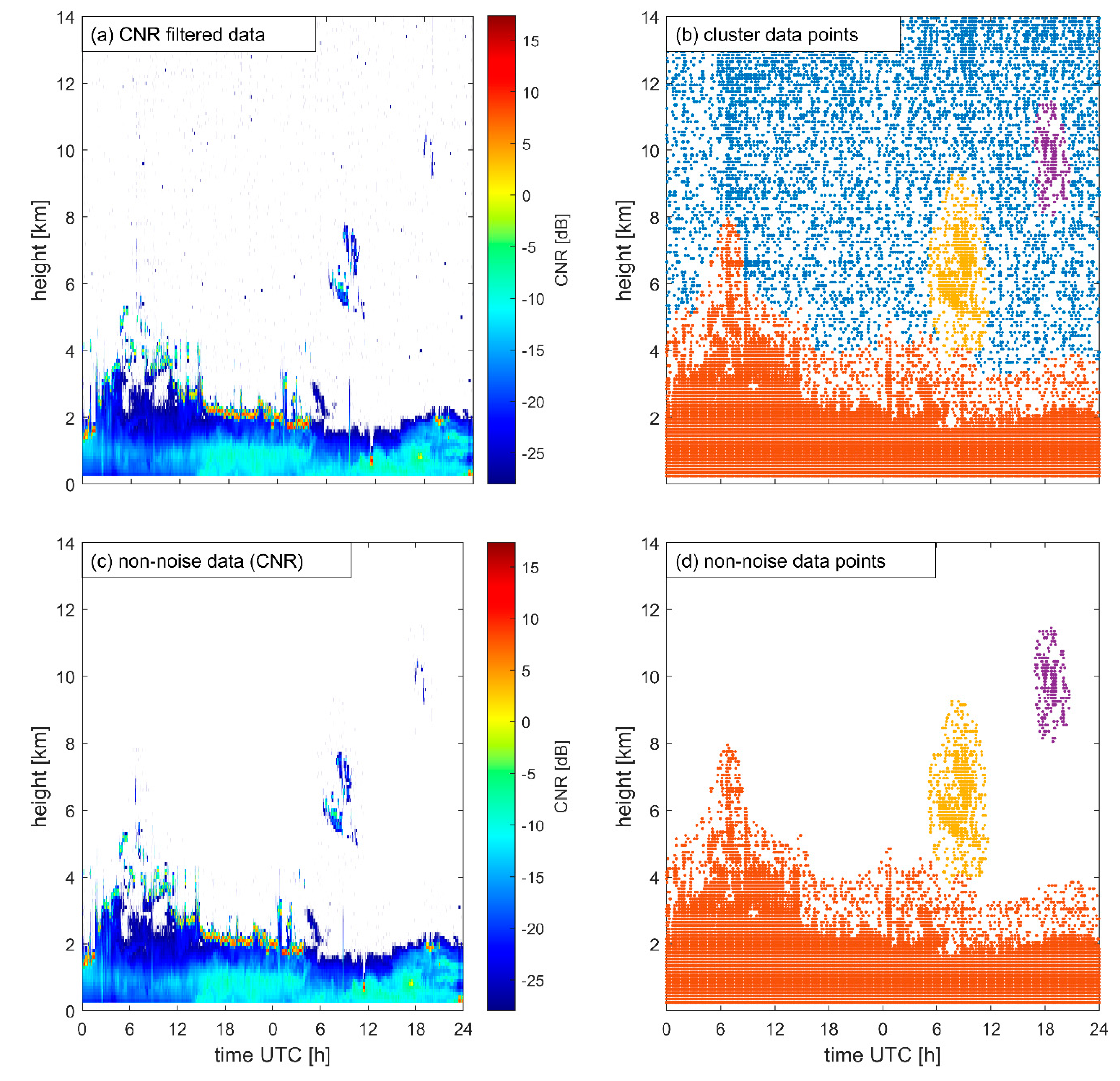
| 2 | High clouds | CNR threshold; DBSCAN clustering | Clouds in the free troposphere and at higher altitudes; separated from other non-noise data; mostly ice clouds, but could be water clouds |
| 3 | Rain | Descending movement; low depolarization ratio | Rain |
| 4 | Aerosol type I | High backscatter coefficient; high depolarization ratio ** | Dust particles in dry atmosphere; relative large size, high concentration with a non-spherical shape |
| 5 | Aerosol type II | Medium-high backscatter coefficient; high depolarization ratio | Dust particles in dry atmosphere; relative small size, low concentration, with a non-spherical shape |
| 6 | Aerosol type III | High backscatter coefficient; medium to high depolarization ratio | Dust particles in a humid atmosphere; relative high concentration, the shape is more spherical |
| 7 | Others | Unclassified data points | Other data points except for noise data |
| 8 | Noise | CNR threshold; DBSCAN clustering | Noise signals |
| Location | Date | CNR of Noise Points (dB) | ||
|---|---|---|---|---|
| Mean | Minimum | Maximum | ||
| Reykjavik * | 06/15/2019 | −34.11 | −41.29 | −10.75 |
| Reykjavik | 07/10/2019 | −33.88 | −41.28 | −12.82 |
| Reykjavik * | 07/31/2019 | −32.40 | −40.25 | −10.75 |
| Keflavik | 07/31/2019 | −33.92 | −49.79 | −12.82 |
Publisher’s Note: MDPI stays neutral with regard to jurisdictional claims in published maps and institutional affiliations. |
© 2021 by the authors. Licensee MDPI, Basel, Switzerland. This article is an open access article distributed under the terms and conditions of the Creative Commons Attribution (CC BY) license (https://creativecommons.org/licenses/by/4.0/).
Share and Cite
Yang, S.; Peng, F.; von Löwis, S.; Petersen, G.N.; Finger, D.C. Using Machine Learning Methods to Identify Particle Types from Doppler Lidar Measurements in Iceland. Remote Sens. 2021, 13, 2433. https://0-doi-org.brum.beds.ac.uk/10.3390/rs13132433
Yang S, Peng F, von Löwis S, Petersen GN, Finger DC. Using Machine Learning Methods to Identify Particle Types from Doppler Lidar Measurements in Iceland. Remote Sensing. 2021; 13(13):2433. https://0-doi-org.brum.beds.ac.uk/10.3390/rs13132433
Chicago/Turabian StyleYang, Shu, Fengchao Peng, Sibylle von Löwis, Guðrún Nína Petersen, and David Christian Finger. 2021. "Using Machine Learning Methods to Identify Particle Types from Doppler Lidar Measurements in Iceland" Remote Sensing 13, no. 13: 2433. https://0-doi-org.brum.beds.ac.uk/10.3390/rs13132433