
A Convolutional Neural Network Based on Grouping Structure for Scene Classification
by
 , , , , and
Xuan Wu
1,2,† ,
,
Zhijie Zhang
3,†,
Wanchang Zhang
1,*,
Yaning Yi
1,2,
Chuanrong Zhang
3 and
Qiang Xu
4 1
Laboratory 5, Aerospace Information Research Institute, Chinese Academy of Sciences, Beijing 100094, China
2
Aerospace Information Research Institute, University of Chinese Academy of Sciences, Beijing 100049, China
3
Department of Geography, University of Connecticut, Storrs, CT 06269, USA
4
State Key Laboratory of Geohazard Prevention and Geo-Environment Protection, Chengdu University of Technology, Chengdu 610059, China
*
Author to whom correspondence should be addressed.
†
Co-first author of the paper.
Remote Sens. 2021, 13(13), 2457; https://0-doi-org.brum.beds.ac.uk/10.3390/rs13132457
Submission received: 10 May 2021
/
Revised: 14 June 2021
/
Accepted: 21 June 2021
/
Published: 23 June 2021
(This article belongs to the Topic High-Resolution Earth Observation Systems, Technologies, and Applications)
Abstract
:Convolutional neural network (CNN) is capable of automatically extracting image features and has been widely used in remote sensing image classifications. Feature extraction is an important and difficult problem in current research. In this paper, data augmentation for avoiding over fitting was attempted to enrich features of samples to improve the performance of a newly proposed convolutional neural network with UC-Merced and RSI-CB datasets for remotely sensed scene classifications. A multiple grouped convolutional neural network (MGCNN) for self-learning that is capable of promoting the efficiency of CNN was proposed, and the method of grouping multiple convolutional layers capable of being applied elsewhere as a plug-in model was developed. Meanwhile, a hyper-parameter C in MGCNN is introduced to probe into the influence of different grouping strategies for feature extraction. Experiments on the two selected datasets, the RSI-CB dataset and UC-Merced dataset, were carried out to verify the effectiveness of this newly proposed convolutional neural network, the accuracy obtained by MGCNN was 2% higher than the ResNet-50. An algorithm of attention mechanism was thus adopted and incorporated into grouping processes and a multiple grouped attention convolutional neural network (MGCNN-A) was therefore constructed to enhance the generalization capability of MGCNN. The additional experiments indicate that the incorporation of the attention mechanism to MGCNN slightly improved the accuracy of scene classification, but the robustness of the proposed network was enhanced considerably in remote sensing image classifications.
1. Introduction
With the rapid advance of remote sensing and earth observation technology, high spatial resolution [1,2] (HSR) remote sensing (RS) imagery with sub-meter level spatial resolution or even very high resolution (VHR) RS imagery [3,4] with centimeter-level resolution became widely available and easily accessible to the public. With the growing amount of data, there is a practical need for a faster and more accurate automated approach to extract their semantic content information and to identify and classify land use and land cover (LULC) types in those images. RS image scene classification [5,6,7] is one crucial way to help alleviate the problem mentioned above since it automatically assigns semantic labels to an RS image scene and has been widely studied due to its vital contributions in land resources planning [8], disaster monitoring [9], urban planning [10], object detection [11], and many other RS applications [12,13,14,15].
Effective feature extraction is one of the key steps in image classification. Traditional machine learning methods need to design features manually and then transform these features into vectors to describe features, such as Scale-invariant Feature Transform (SIFT) features [16]. Combined with clustering methods like K-Means, these features are mapped into a visual dictionary and generate a feature histogram for each image with bag of visual word (BOVW) [17]. However, this method relies heavily on handcrafted features, and the clustering method also requires expert experience and knowledge. In recent years, the convolutional neural network has achieved remarkable progress in natural image classification. AlexNet [18] used a large number of convolution kernels for feature extraction, while VGGNet [19] further increased the width and depth of the network and enlarged the model volume. GoogLeNet [20] used convolution kernels of different sizes to construct the inception structure, it can extract multi-scale features and used the global pooling layer to replace the full connection layer, which reduced the amount of computation and improved the performance of the network. ResNet [21], committed to solving the problem of vanishing gradient when the network is too deep, used the residual structure to solve the problem of model degradation. The newly emerged attention mechanism also promotes the development of deep learning; it can learn new features based on the input features, so as to improve the network performance. The following networks all adopted the advantages of the previous networks and got improved based on them: DenseNet [22] integrated the features of the front layer, SENet [23] defined the channel weight relationship, strengthened the useful information, and suppressed the useless information. SKNet [24] used multi-scale convolution and can adaptively adjust the convolution feature map’s weight. ResNeXt [25] was among the first ones that attempted to use multiple groups of convolutions for feature extraction.
Compared with natural images, remote sensing image scenes are more complex, a single scene is usually mixed with many different kinds of objects [26,27,28]. Due to the inconsistency of spatial resolution, the objects’ spatial scales are not the same. Some ground objects may have significant similarities in the spectrum [29,30]. Therefore, methods that ensure the model extract effective features are the focus and also the difficulty for remote sensing image scene classification. At present, the feature extraction in remote sensing image scene classification research is mainly developed on the basis of CNN models. Han et al. [31] improved a pre-trained AlexNet with spatial pyramid pooling (SPP) that was used for feature fusion. Gong et al. [32] introduced an anti-noise transfer network based on pre-trained VGGNet. Li et al. [33] were inspired by the inception structure of GoogleNet and designed a multi-scale feature extraction method which is used to solve the problem of the object size varying considerably in the same category image. The attention mechanism, therefore, was designed to change the weight of feature maps to improve network performance [34,35]. Since then, spatial and channel attention mechanisms were applied to feature extraction [36,37,38,39]. However, these methods still have some disadvantages. On the one hand, Multi-scale features can be expanded by the superposition of several small convolutional kernels. On the other hand, these models do not yet take process of network internal feature extraction into account. Therefore, it is necessary to understand the details of feature extraction by tremendous amount of convolutional kernels.
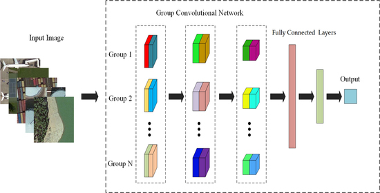
To discern the internal feature extraction process of the model, we proposed MGCNN models that embed group convolution blocks in each convolution layer and used ResNet-50 [20] as the backbone network structure to account for this issue in the present study. The grouping process was designed to divide the input into different groups to perform convolution separately in each group, and then to combine each group’s convolutional results to improve the performance of the model in scene classifications. In group convolution blocks, we introduced hyper-parameter C to control the number of groups and paths. The number of paths, which affected the accuracy of the model through several experiments, was regarded as hyper-parameter. To further explore the performances of attention mechanism in remote sensing scene classifications, we introduced attention structure into MGCNN and formed a variation of MGCNN, called MGCNN-A. This structure can automatically train the weight of the feature maps based on grouping convolution. In short, the major works with scientific contributions we made in this study were summarized below:
- A convolutional neural network framework, namely MGCNN, was proposed based on group convolution scheme by introducing a hyper-parameter C to divide the feature extraction path into multiple channels for improving efficiency of feature extraction meanwhile enriching the feature space.
- Attention mechanism and group convolution scheme was explored and incorporated into the proposed MGCNN, and a modified MGCNN, namely MGCNN-A, was developed. The influence of incorporating grouping and attention mechanism in feature extraction on the performance of MGCNN-A, as well as the effects of hyper-parameters C being introduced in the model under the fixed feature map channel numbers, were comprehensively investigated. At the same time, the features extracted by MGCNN and MGCNN-A are compared by discussions.
The rest of this paper is organized as follows. In Section 2, we introduce the proposed MGCNN and MGCNN-A in detail. Experiments and results with our proposed models on two datasets are given in Section 3. In Section 4, discussions about the proposed model are presented, followed by the conclusion and future work which are discussed in Section 5 at the end.
2. Methodology
2.1. Framework of Model
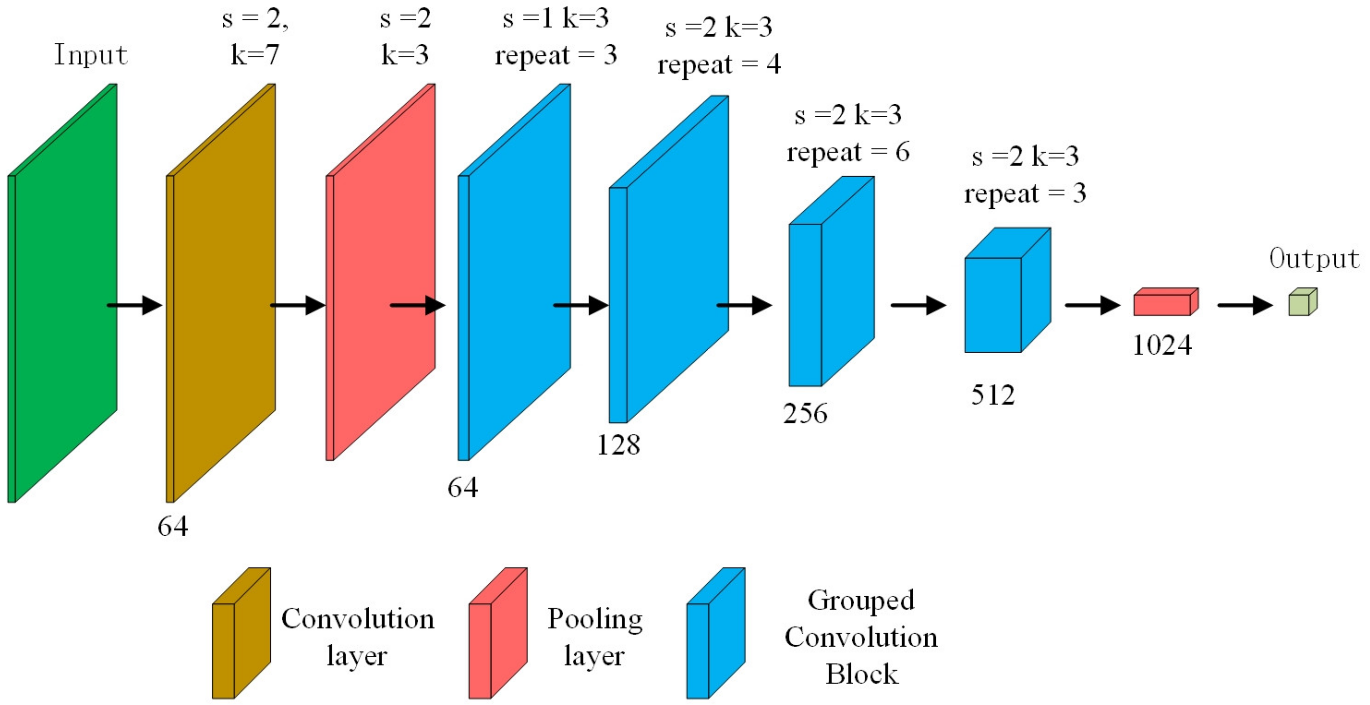
As shown in Table 1, ResNet-50 [20], was adopted as a backbone architecture to develop our proposed models MGCNN and MGCNN-A. In the original ResNet-50 [20], the number of convolution kernels in each layer was 64, 64, 128, 256, 512, respectively. As shown in the third column of the Table 1, we reduced the number of convolution kernels to avoid over fitting. In our proposed models, grouped convolution and grouped attention blocks were embedded into each convolutional layer of MGCNN and MGCNN-A to enrich the features extracted. Finally, we used global average pooling to replace the fully connected (FC) layers to reduce the number of parameters. The parameter C indicates that the input tensor is divided into C groups, while A indicates that the attention structure is added to each group. Figure 1 illustrates the size of output tensor after convolution of each layer. The parameter k in the graph is the convolution kernel size, s is the stride size and repeat is the number of grouped attention block. The last four convolution layers are composed of several convolution blocks (blue block), in which grouped convolution block and grouped attention block are used.
2.2. Grouped Convolution Block
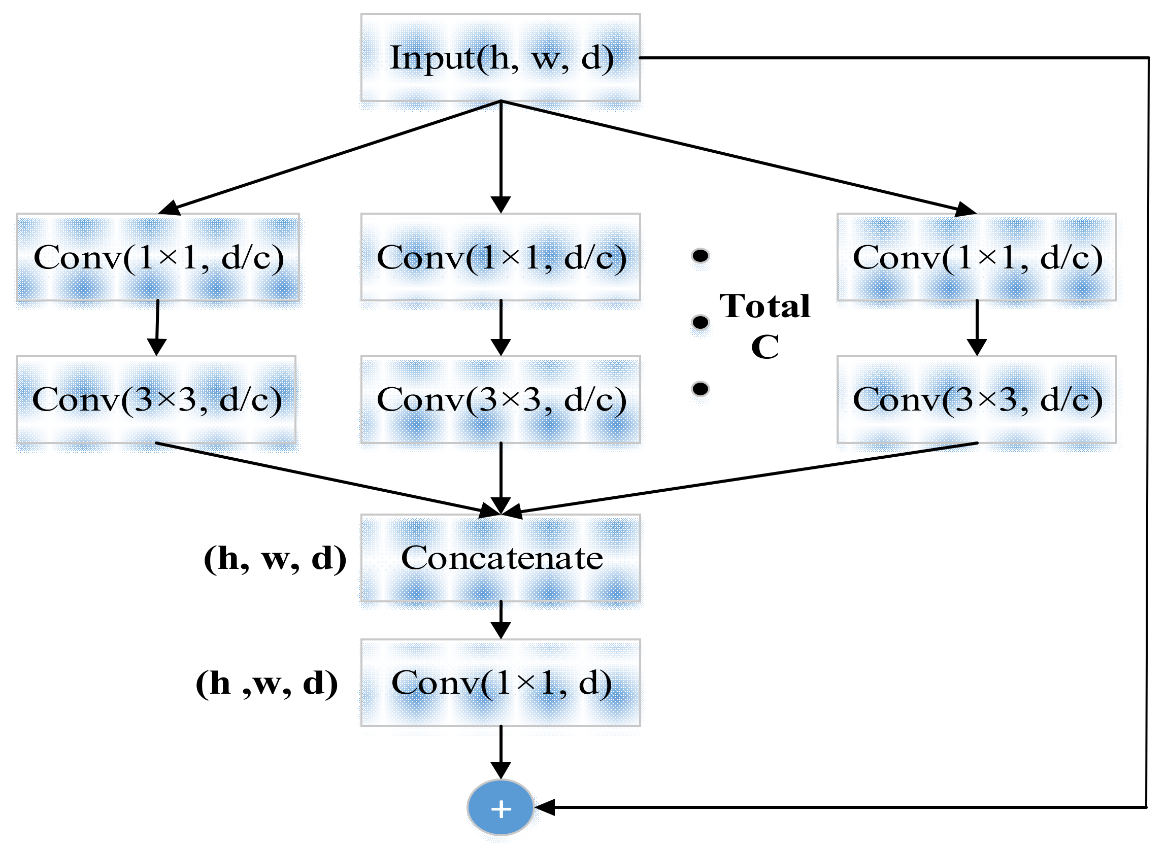
Grouped convolution was first used in AlexNet [17], which utilized two GPUs for training the model. According to our experiments, multiple paths were thought favorable for extracting features efficiently. As shown in Figure 2, we added a hyper-parameter C representing the number of groups to divide the input tensor into several groups. In each group, we used a 1 × 1 kernel succeeding a 3 × 3 convolution kernel to transform feature maps. After convolution layers, the RELU activation function was applied to adjust the model. Afterwards, a concatenation function was used to combine the outputs from each path. Finally, we complimented the output of a 1 × 1 convolution layer to the input to construct the structure of the short-cut in ResNet [20].
2.3. Grouped Attention Block
2.3.1. Channel Attention
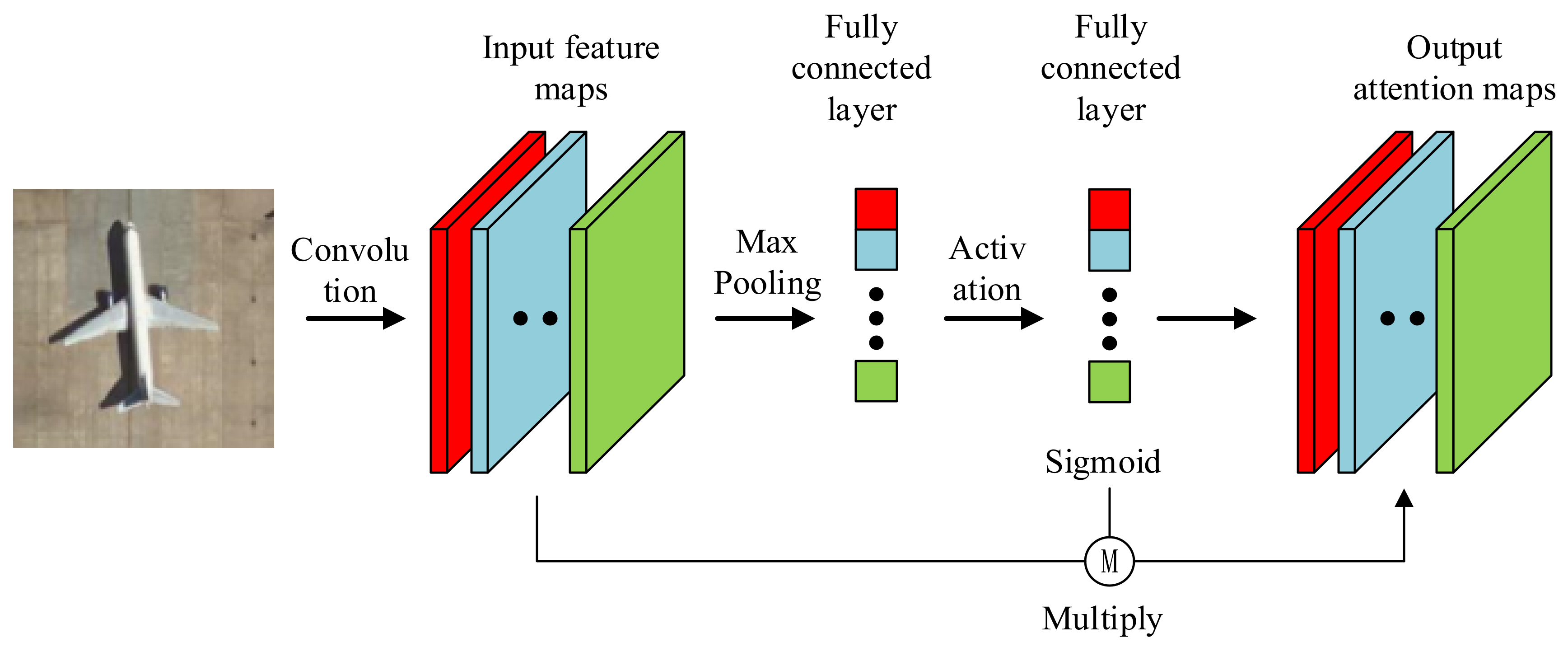
In typical convolution neural networks, the weight for each feature channel is set consistent and usually can only discriminate prominent features. The channel attention structure can automatically train different weights according to different feature maps. As shown in Figure 3, two fully connected layers were designed to learn the weights of neurons, while convolution layers were used to obtain feature information. As a final step, the multiplied outputs of weight for each feature channels were optimized by Sigmoid function and input feature maps were considered as reinforced attention maps. The attention module can be expressed as follow:
where AS and AR denote activation function of Sigmoid and RELU, and W1,2 and f1,2 refer to the two convolution layers and the two fully connected layers, correspondingly. As can be seen from the formula, input X will be transformed into a feature map after convolution layers. The fully connected layers synthesized the feature maps and were activated by RELU and Sigmoid, which amplified the high-frequency signal. Besides, the multiply of the fully connected layers and corresponding channels magnified the more prominent features.
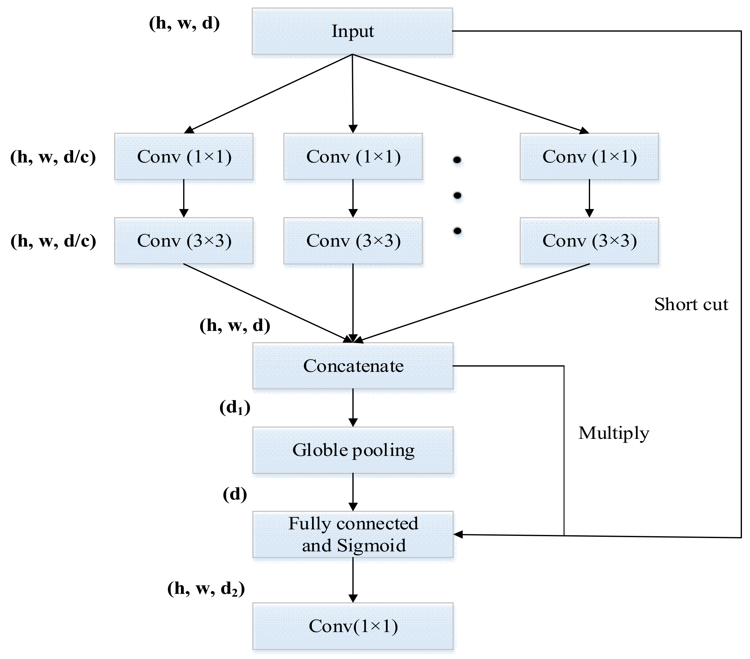
2.3.2. Grouped Attention Block
Although the attention structure is capable of automatically training the weight of each attention channel, it is challenging to enrich the space of feature maps solely relying on it. Thus, the grouped attention blocks with grouped parameter C were introduced to the attention structure, which structure is displayed in Figure 4. Parameter C that we added here was used to divide each convolution layer into C paths. In each attention group, same as the grouped convolution block, one 1 × 1 succeeding one 3 × 3 convolution kernels were used. After grouped convolution, grouped feature maps were concatenated and stretched into a fully connected layer which was weighted to grouped feature maps. Finally, we adopted the shortcut structure of ResNet [20] and added the convolution result to the input layer.
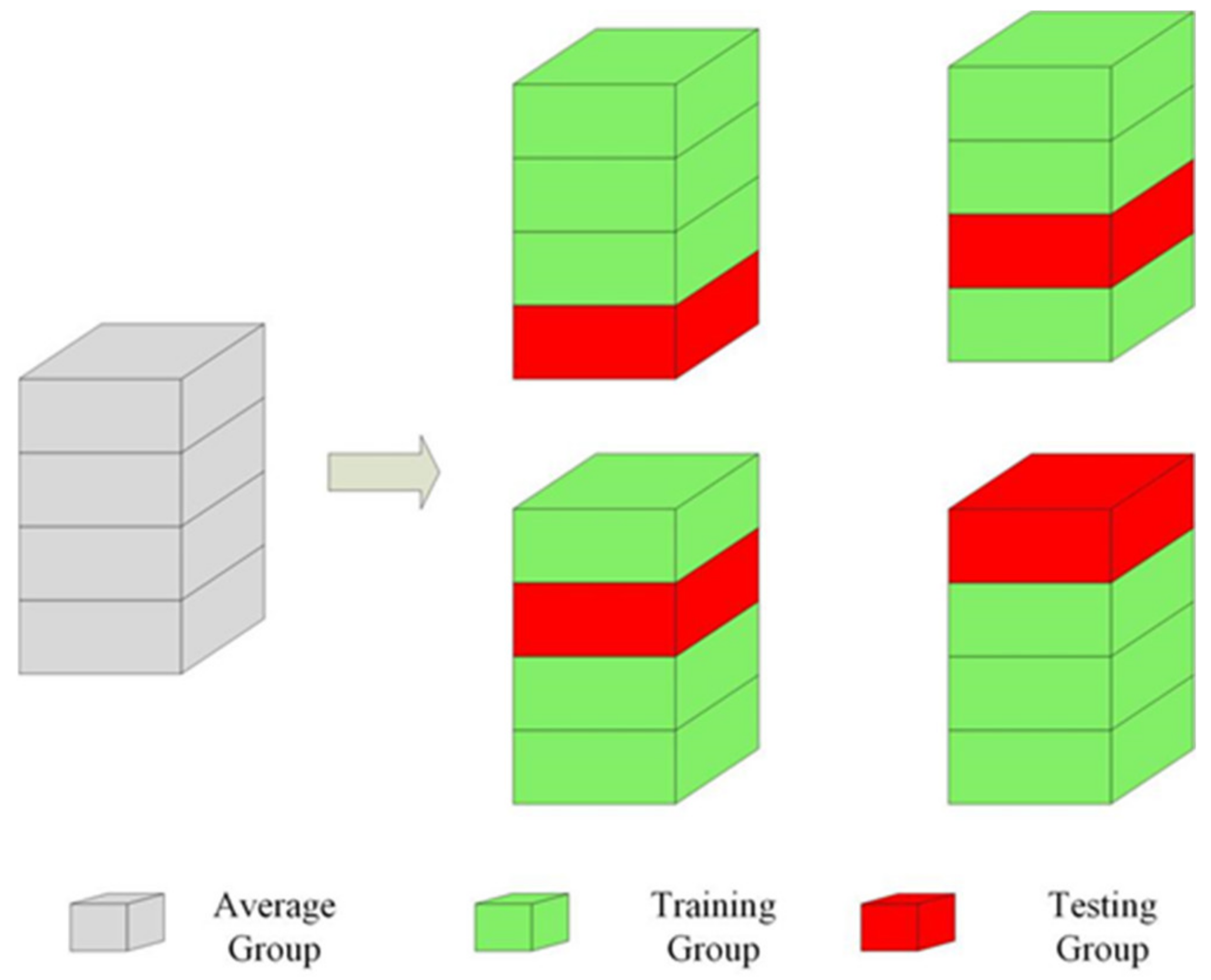
2.4. Data Augmentation and Cross Validation
The cross-validation method, as illustrated in Figure 5, was adopted to prove the validity of our model. The datasets were randomly divided into four groups for cross-validation purposes: three for training and one for validation. In other words, we trained each model four times and recorded the average of the accuracy. Cross-validation can effectively avoid the problem of high or low accuracy in some specific datasets. This method was implemented in RSI-CB [40] and UC Merced Land Use [41] datasets.
The number of images varies from 198 to 1331 within each category of the RSI-CB dataset. The imbalance of data volume between each category will lead to the model being more inclined to classify an image from a low-volume category as an image from high-volume categories, so the training loss can be reduced. Nevertheless, this would negatively affect the performance of our proposed model; therefore, several algorithms [42], including crop, rotate, flip, and so on, were used to balance the volume between each category. Through the preliminary experiment, it was observed that there was a severe over fitting problem when three-fourths of the UC Merced Land Use dataset was used for training. This indicated that with small training data it was difficult to reflect the actual distribution of categories. Data augmentation methods can eliminate the amount of random noise that was easily learned by the neural network in a small dataset.
2.5. Overall Accuracy and Confusion Matrix
The overall accuracy (OA) is an index to measure the proportion of correct prediction individuals in the whole test data set, which can well reflect the quality of the model. In the confusion matrix, each row represents the actual category, and each column represents the forecast category. It can easily reflect the result of wrong and missing points of each category. The way for the calculation of OA can be expressed as follow:
where Pij is the correct prediction of individual, and n, k represents the total number of each category and the total number of categories. T is the total number of test data set.
3. Experiments and Result
3.1. Datasets
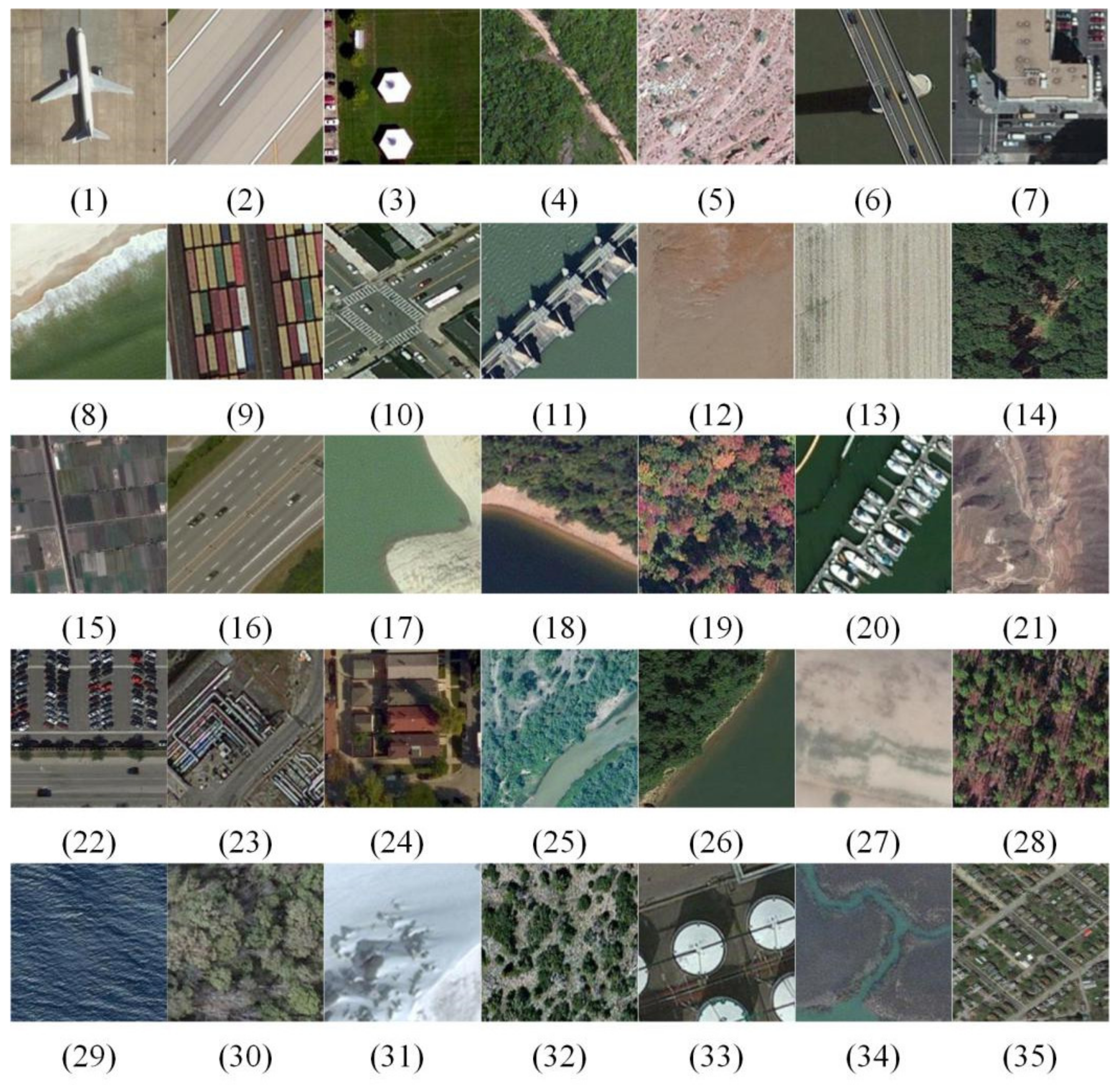
To evaluate the performance of the proposed model, RSI-CB and UC-Merced datasets were used as benchmarks for model training. Two introduced hyper-parameters C were tuned on the RSI-CB dataset. The effectiveness and performance of our proposed networks were tested on a smaller dataset, i.e., the UC-Merced dataset. The RSI-CB dataset contains 35 categories with 24,747 images in total. Images were not evenly distributed among 35 categories, with 1331 images within a single category as the maximum and 198 as the minimum. Each image in the dataset has a 0.3–3 m spatial resolution with a dimension of 256 × 256 pixels. Sample images of each category within this dataset are shown in Figure 6.
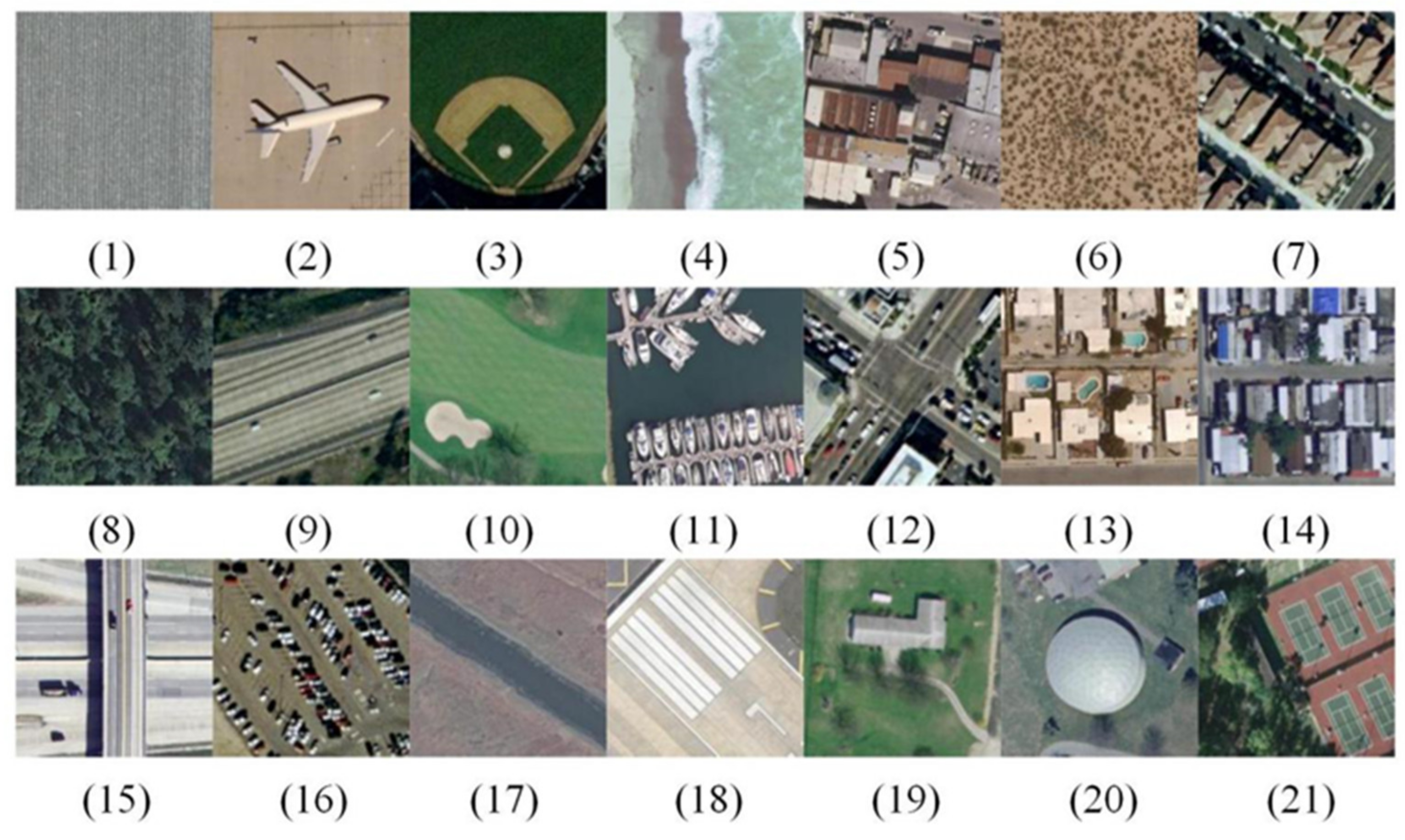
The UC-Merced Land Use dataset is widely used as a benchmark dataset for evaluating the performance of deep learning models regarding tasks of remote sensing scene classification. It consists of 21 categories with 100 pictures in each category. Each picture has a 0.3 m spatial resolution with a dimension of 256 × 256 pixels. Figure 7 exhibits sample images of each category in this dataset.
3.2. Experimental Setup
The experiments were implemented under the Tensorflow framework on an NVIDIA GeForce RTX 2080Ti GPU. Data augmentation algorithms were applied to all images, and all images were cropped to 256 × 256 pixels for model input. We used a gradient descent optimizer with a decaying learning rate. The initial learning rate was 0.1, the exponential decay rate was 0.96 every 300 iterations, and the batch size was 32. The maximum iteration was set to 40,000.
3.3. Experimental Results
3.3.1. Experiment on RSI-CB Dataset
Data Augmentation Comparative Experiment
Table 2 lists overall accuracy (OA) between the performances applying and not applying data augmentation on three different base networks. It can be noted that data augmentation posed more significant effect on VGGNet-16 (8% increase) compared to the other two networks (about 2% increase respectively). Moreover, ResNet-50 achieved the highest OA (94.930%), about 1.139% higher than the network ranked in second for OA: GoogLeNet-22 (93.791%). Although VGGNet-16 benefited the most from data augmentation, its OA was significantly lower than the other two networks.
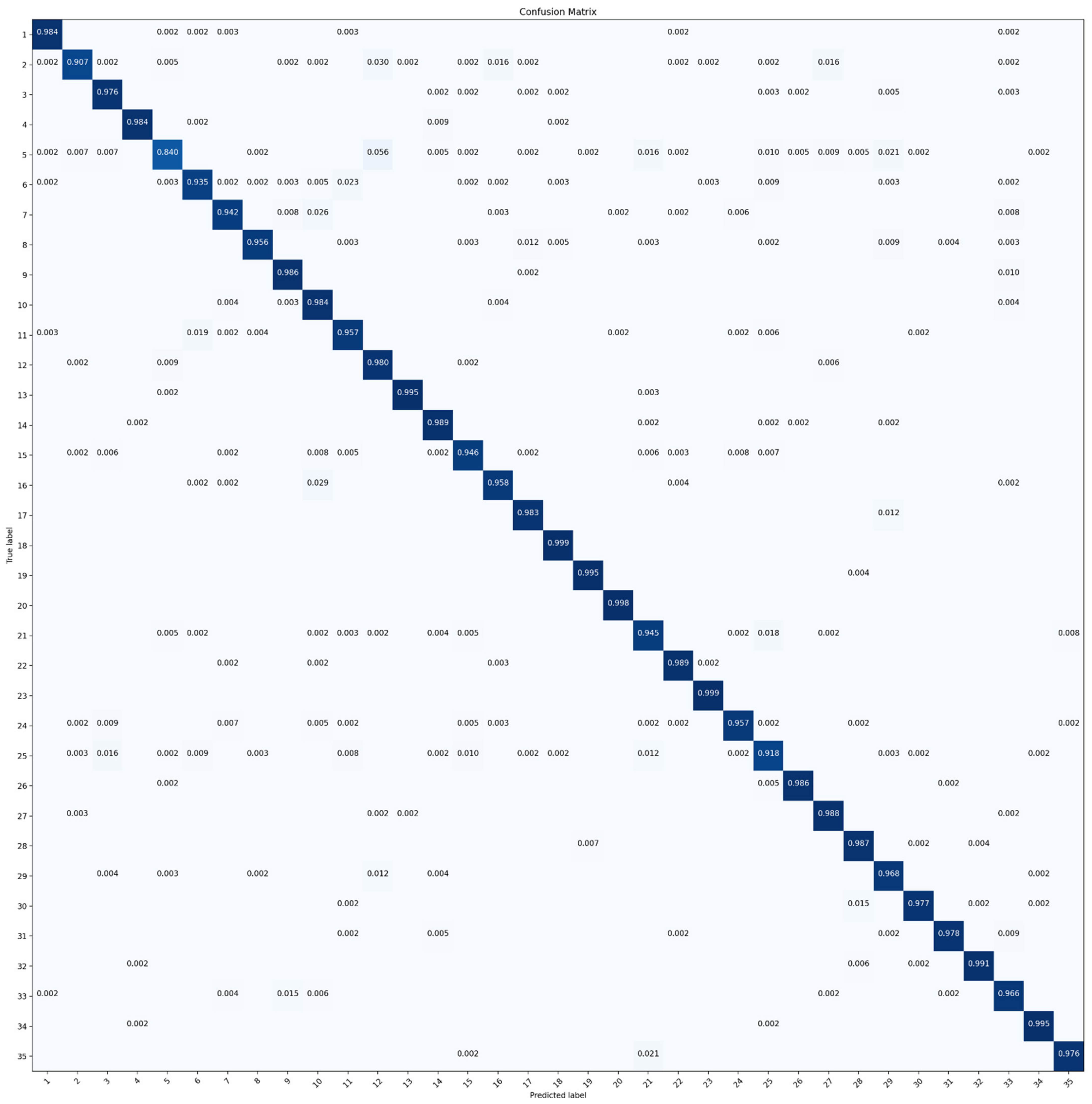
Figure 8 exhibits a confusion matrix (CM) of ResNet-50 that ignored accuracy below 0.001. It was evident that the model was not able to recognize bare land (class 5) from the desert (class 12). Both of them obtained lower accuracy compared to the others. Slight confusions also existed between other categories since OA was calculated as the combined average accuracy of each category.
MGCNN Experiment
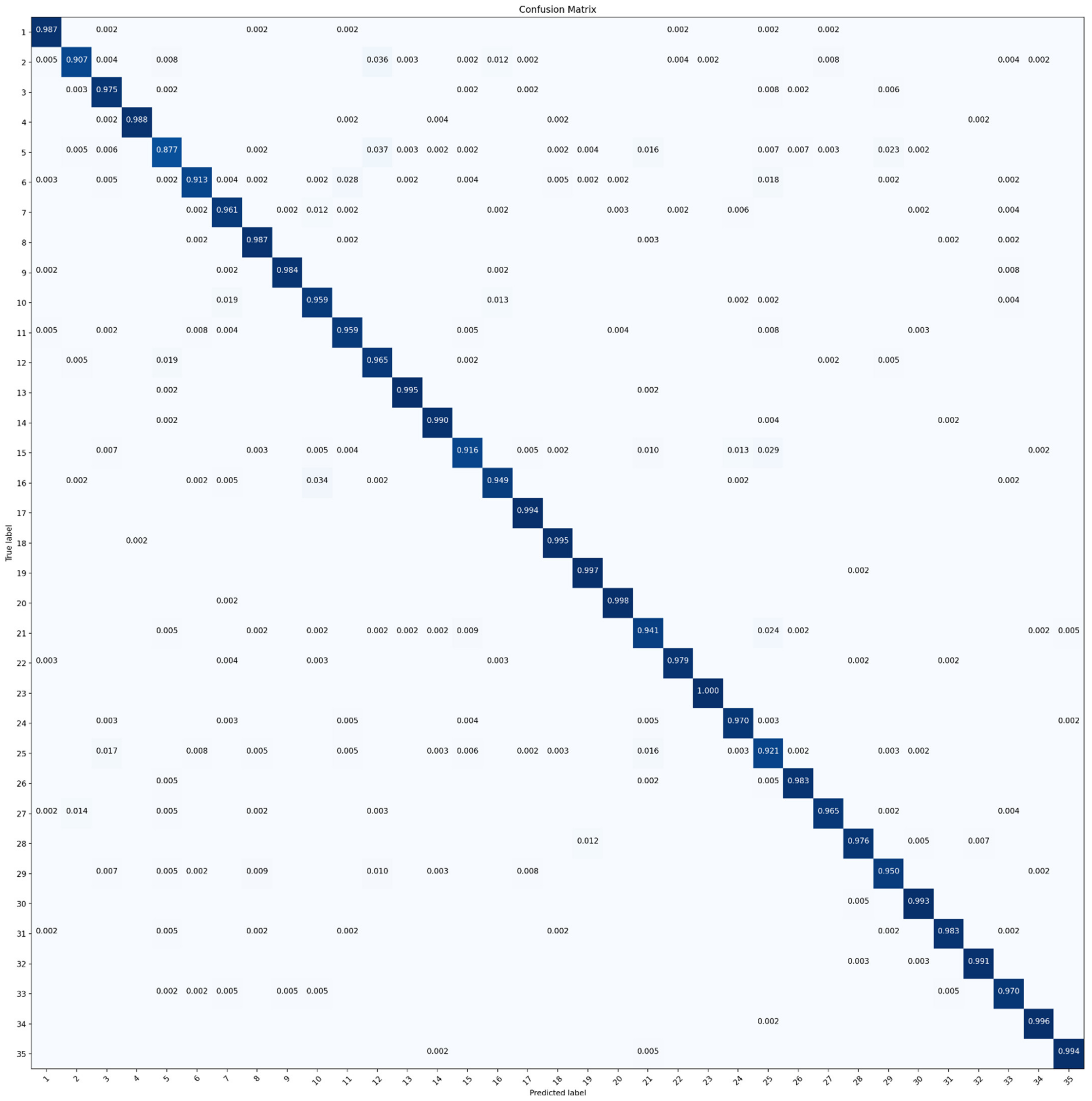
Hyper-parameter C is the core parameter of the MGCNN model. It can be observed from Table 3 that grouping can improve performance. OA increased by about 2% after grouping compared with MGCNNs and ResNet-50. Specifically, the highest OA was obtained by MGCNN-C4 (96.881%), slightly higher than that of MGCNN-C2 (96.859%). The obtained OA of MGCNN-C8 and MGCNN-C16 suggested that too many groups embedded in the neural network did not lead to better performance of the network. The CM of MGCNN as shown in Figure 9 indicates that the accuracy obtained for bare land (class 5) and river (class 25) are lower than those of other categories with MGCNN.
MGCNN-A Experiment
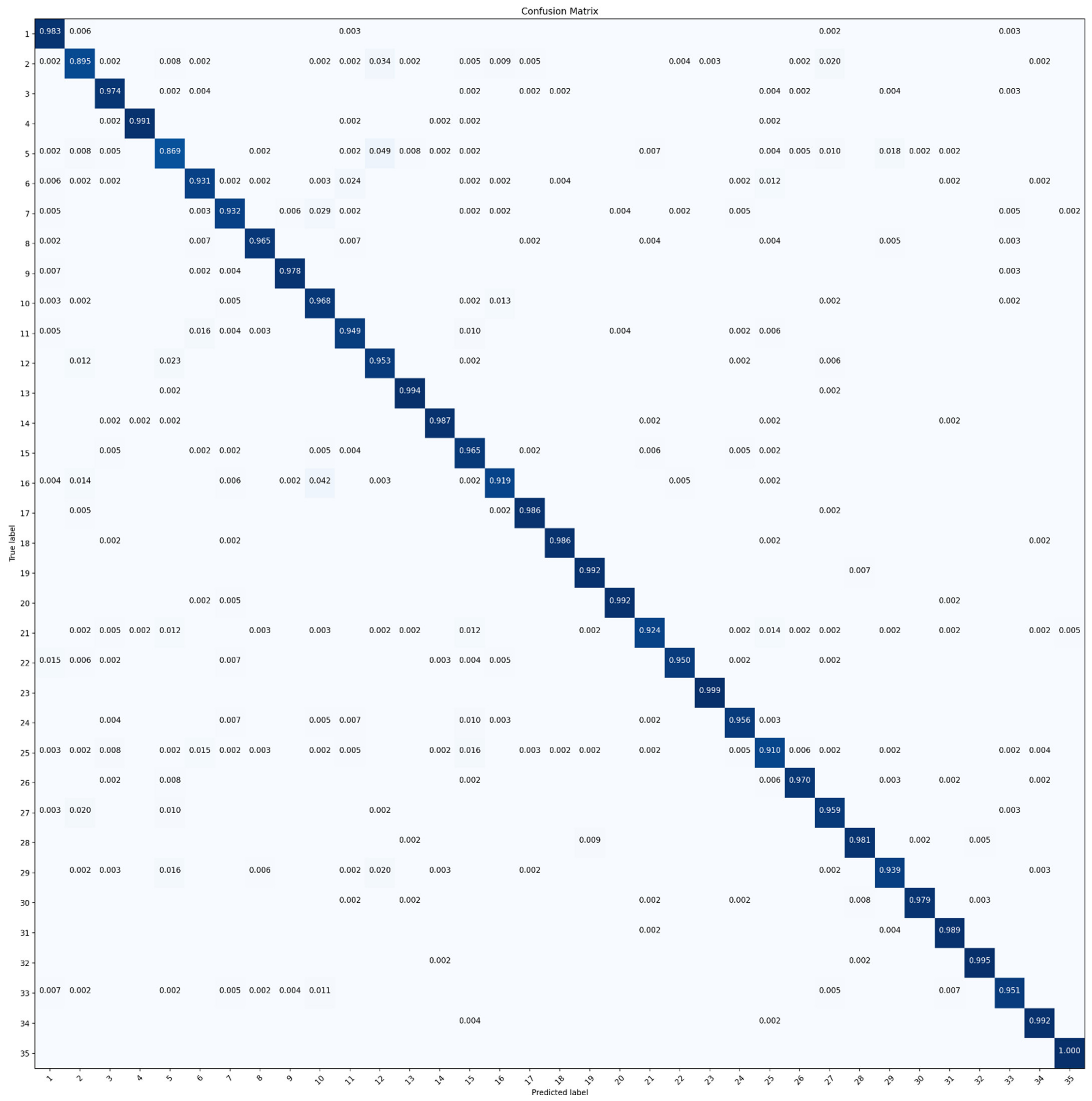
To further explore the performance of grouping, we added the now trending attention structure to this new model. The OA of MGCNN-A with different combinations of hyper-parameter C is shown in Table 4. The best performance among combined models of MGCNN-A and attention structure, which was MGCNN-A4, only obtained a 1.36% performance gain compared to ResNet-50. The decline of OA can be attributed probably to that with the number of groups increases, the depth of the feature map extracted from each group becomes smaller. In general, attention structure seemed not work well in MGCNN-A. Figure 10 presents the CM of MGCNN-A4 obtained through experiments described previously.
3.3.2. Experiment on UC-Merced Dataset
Data Augmentation Comparative Experiment
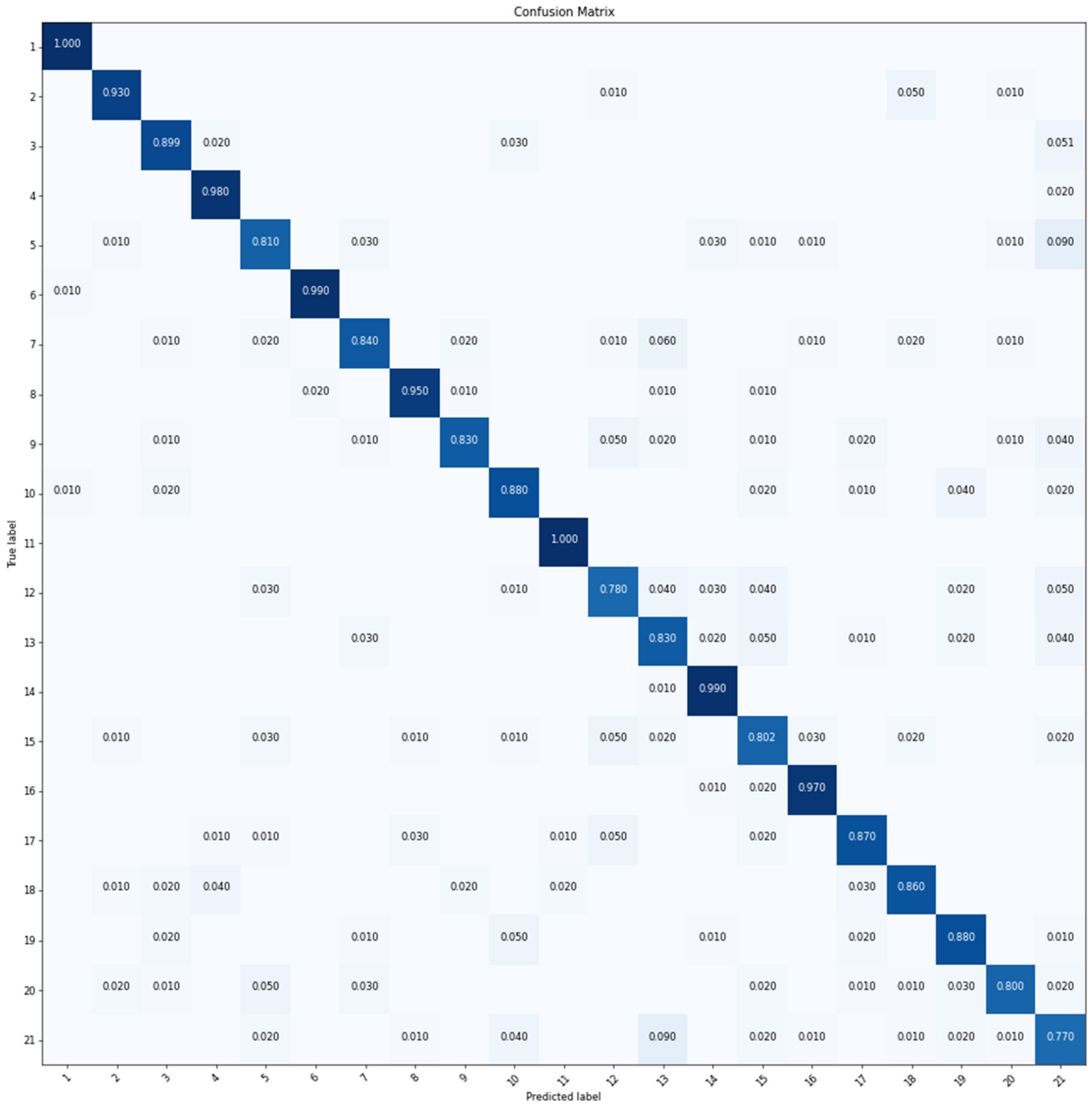
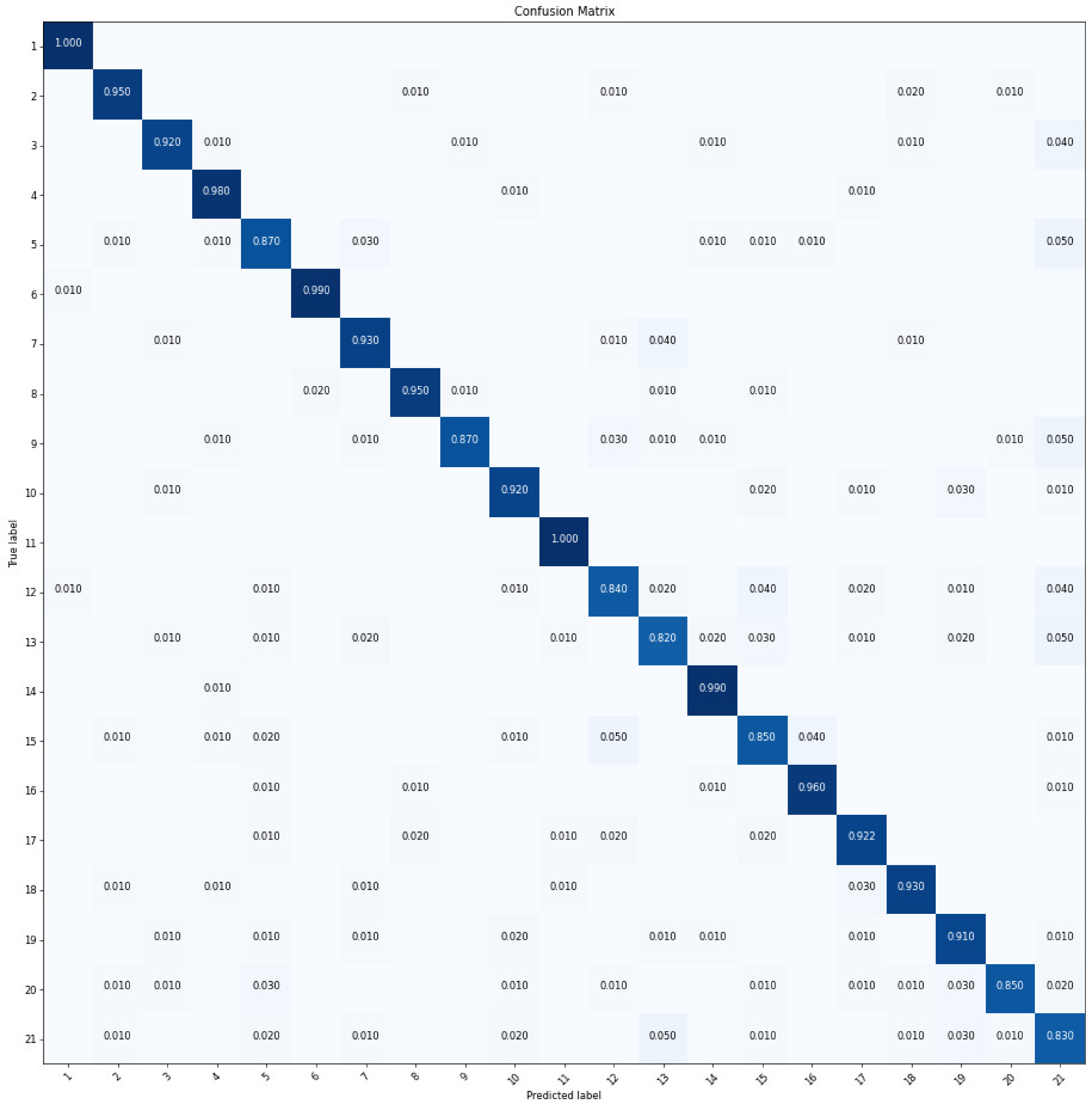
As shown in Table 5, data augmentation can effectively improve the classification accuracy among the three models. The OA of GoogLeNet-22 and ResNet-50 increased by about 7%, while VGGNet-16 only increased by 3%. ResNet-50 performed the best among the three models. It can be observed that in Figure 11, the agricultural (class 1), beach (class 4), chaparral (class 6), forest (class 8), harbor (class 11), mobile home park (class 14), and river (class 16) are classified almost 100% in accuracy. The other scenes are classified about 85% in accuracy except for intersection (class 12) and tennis court (class 21).
MGCNN Experiment
We also tested our model with the UC-Merced dataset. Table 6 lists the OA of MGCNNs achieved in the experiment, which about 2% increase of accuracy can be observed after grouping. MGCNN-C4 achieved higher OA than other groups, which was attributed to too many groups might reduce the model’s efficiency, this was also demonstrated by MGCNN-C16. It is observed from Figure 12 that MGCNN-C4 achieved more than 95% accuracy in classification of agricultural (class 1), airplane (class 2), and six other scenes. Meanwhile, the errors of the classified buildings (class 5), dense residential (class 7), intersection (class 12), and other categories are reduced by around 5% compared to those of the ResNet-50 after grouping.
MGCNN-A Experiment
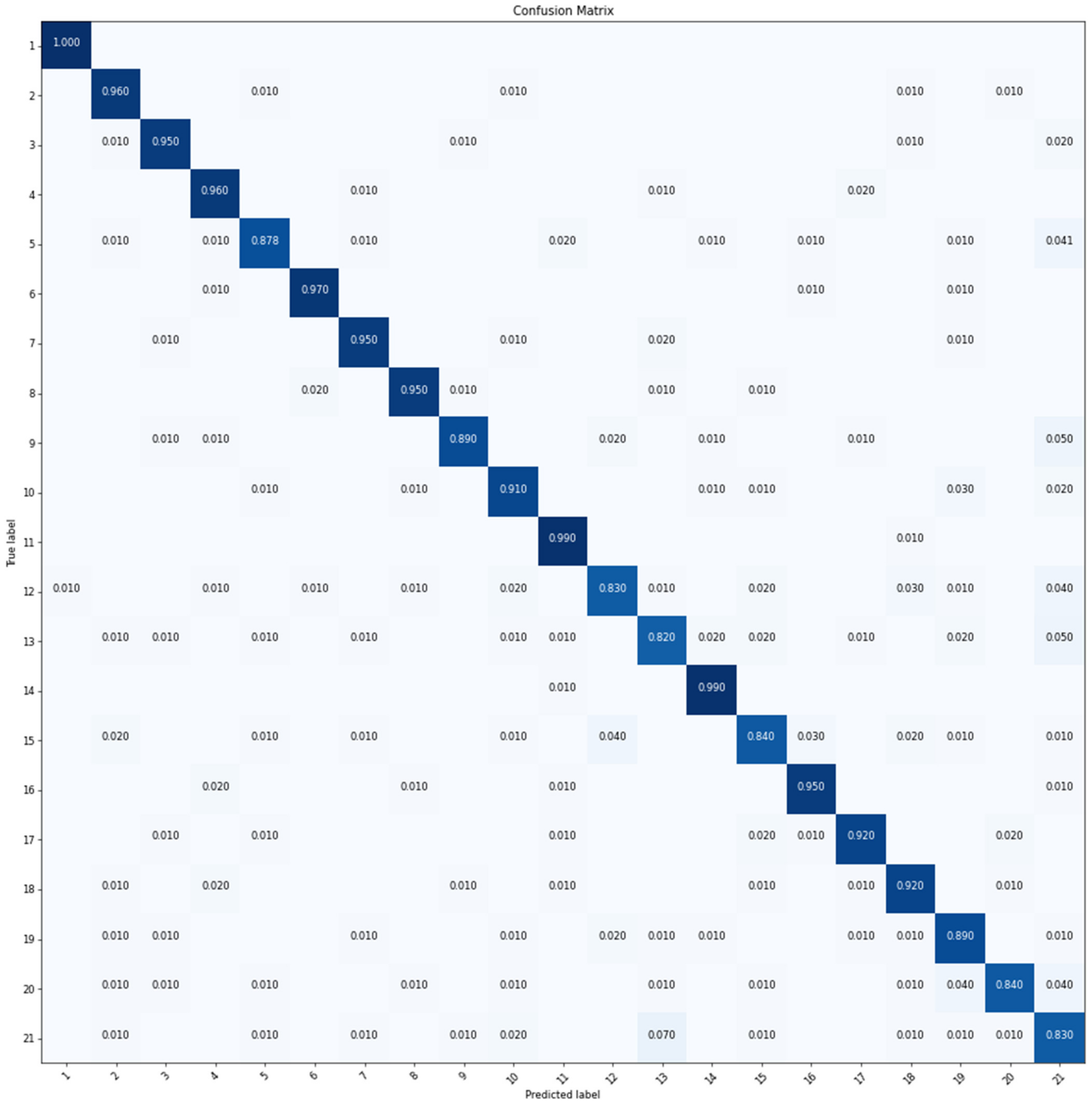
We investigated the performance of MGCNN-A with the UC-Merced dataset either, and the OA achieved in this experiment was listed in Table 7. It can be seen from Table 7 that all MGCNN-A models outperformed the ResNet-50, and the MGCNN-A models benefited from grouping with increased OA about 2% in general. Different grouping methods in MGCNN-A had promoted the model performances around 1.5% regarding achieved OA, among which MGCNN-A4 gained the most benefit on OA increase. It is worthwhile mentioning that attention structure made less impact on OA compared to groupings. The CM of MGCNN-A4, as shown in Figure 13, reveals that some of the scenes are mixed up in classifications by MGCNN-A4, such as buildings (class 5), container (class 9), medium residential (class 13), and tennis court (class 21).
4. Discussions
4.1. Generalization Capability
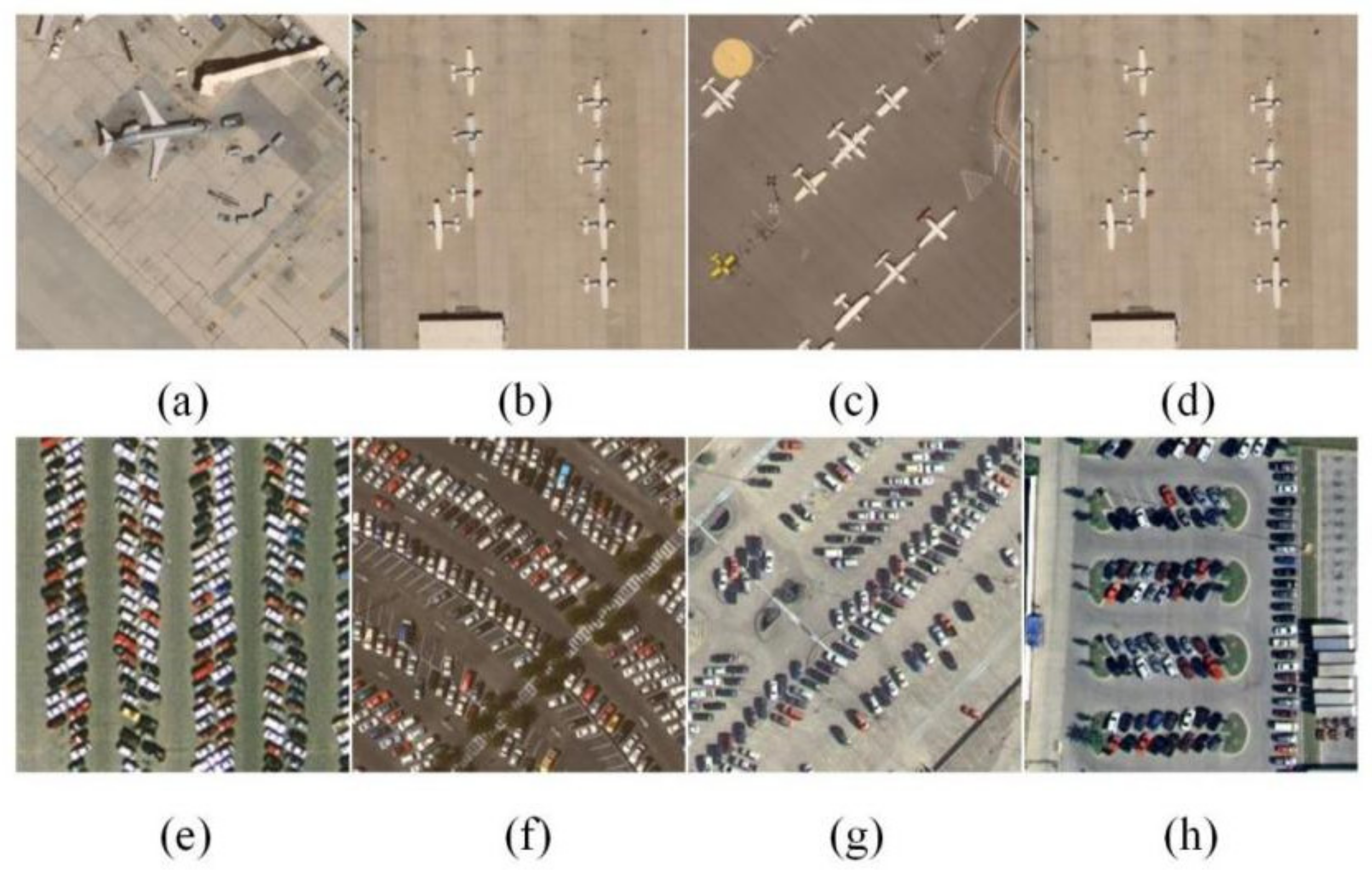
Through the above experiments, we found that the grouping convolution could effectively improve the classification accuracy. Meanwhile, the classification accuracy of MGCNN-A with attention mechanism did not seem to have effect in the two datasets. We tested the proposed model between the two datasets. Airplanes and parking lots are the two same categories defined in RSI-CB and UC-Merced datasets. We trained our models with the RSI-CB dataset and then validated our models with the UC-Merced dataset to test generalization capability of our models by classification focused on these two categories. Both MGCNN and MGCNN-A outperformed the ResNet-50 in this experiment, and MGCNN-A4 performed better than MGCNN-C4 as indicated otherwise from previous experiments and exhibited stronger robustness when transferring the model to validate with a different dataset, which was most probably due to the enhanced local obvious features for classification by attention mechanism of the MGCNN-A. Table 8 shows the OA of the three models in the Airplane and Parking lots categories. Figure 14 presents the image scenes that both models failed to identify. It is obvious that smaller objects are more challengeable to be recognized by all three DL models. The reason for this is that pooling layers tended to ignore details.
4.2. Feature Extraction
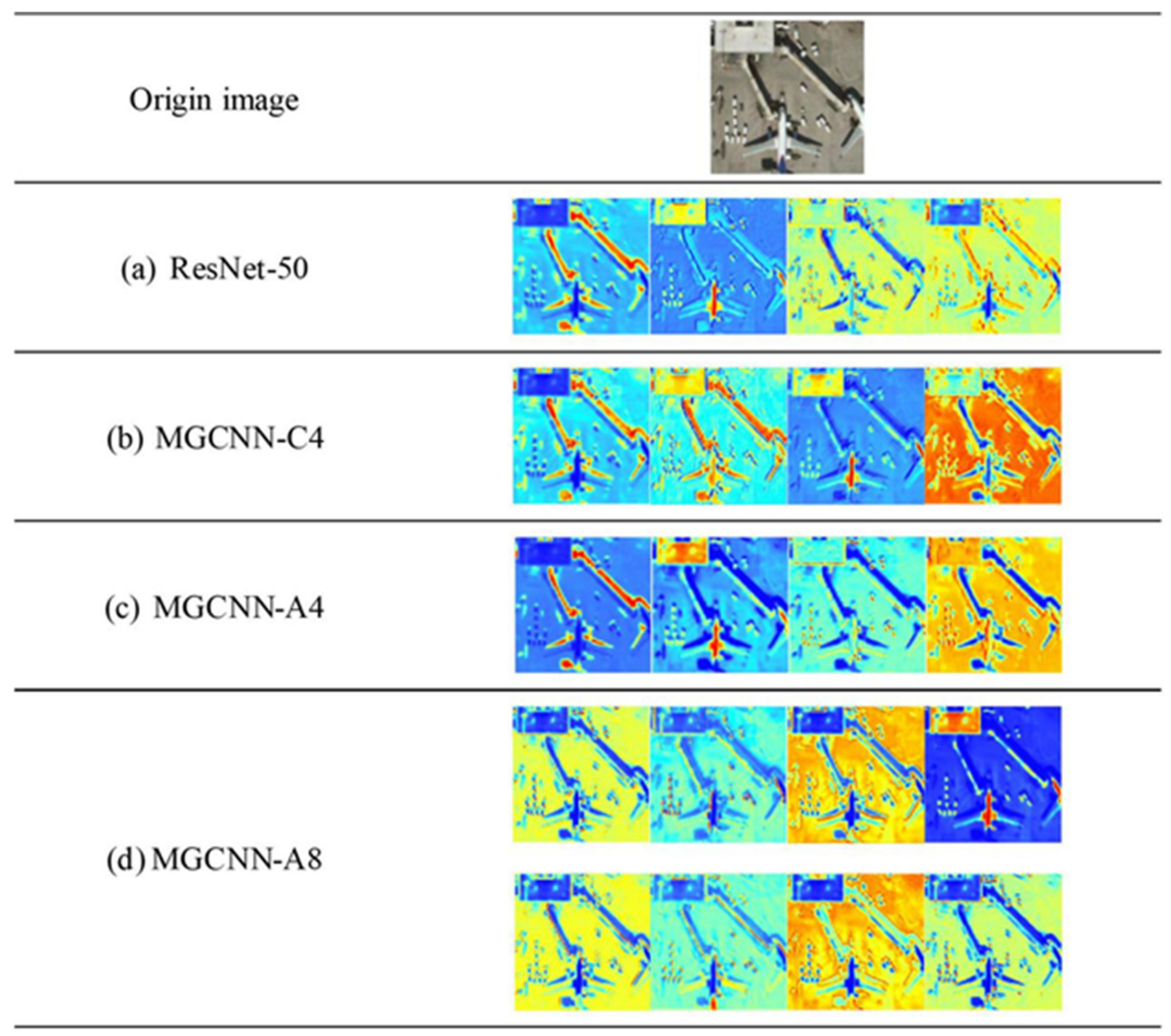
In order to better understand the performance of our model in feature extraction, we visualized the feature layer of the model. As shown in Figure 15a, ResNet-50 extracted some repetitive features. For example, the last two feature maps are very similar. On the contrary, the four groups of feature maps extracted by MGCNN-C4 are more abundant in humble information, which distinguishes the background and scene features of the image (such as aircraft and house) well. In MGCNN-A4, the attention structure in the model enhanced the features more apparent in the image. For example, the features extracted were clearer for the objects with edges easier to recognize in the image. For better understanding why the models’ accuracy decreased as the number of grouping increases, we visualized eight groups of the extracted feature maps from MGCNN-A8 as presented in Figure 15d; half of the feature maps are analogous, and the extracted features are very similar to MGCNN-A4.
4.3. Limitations
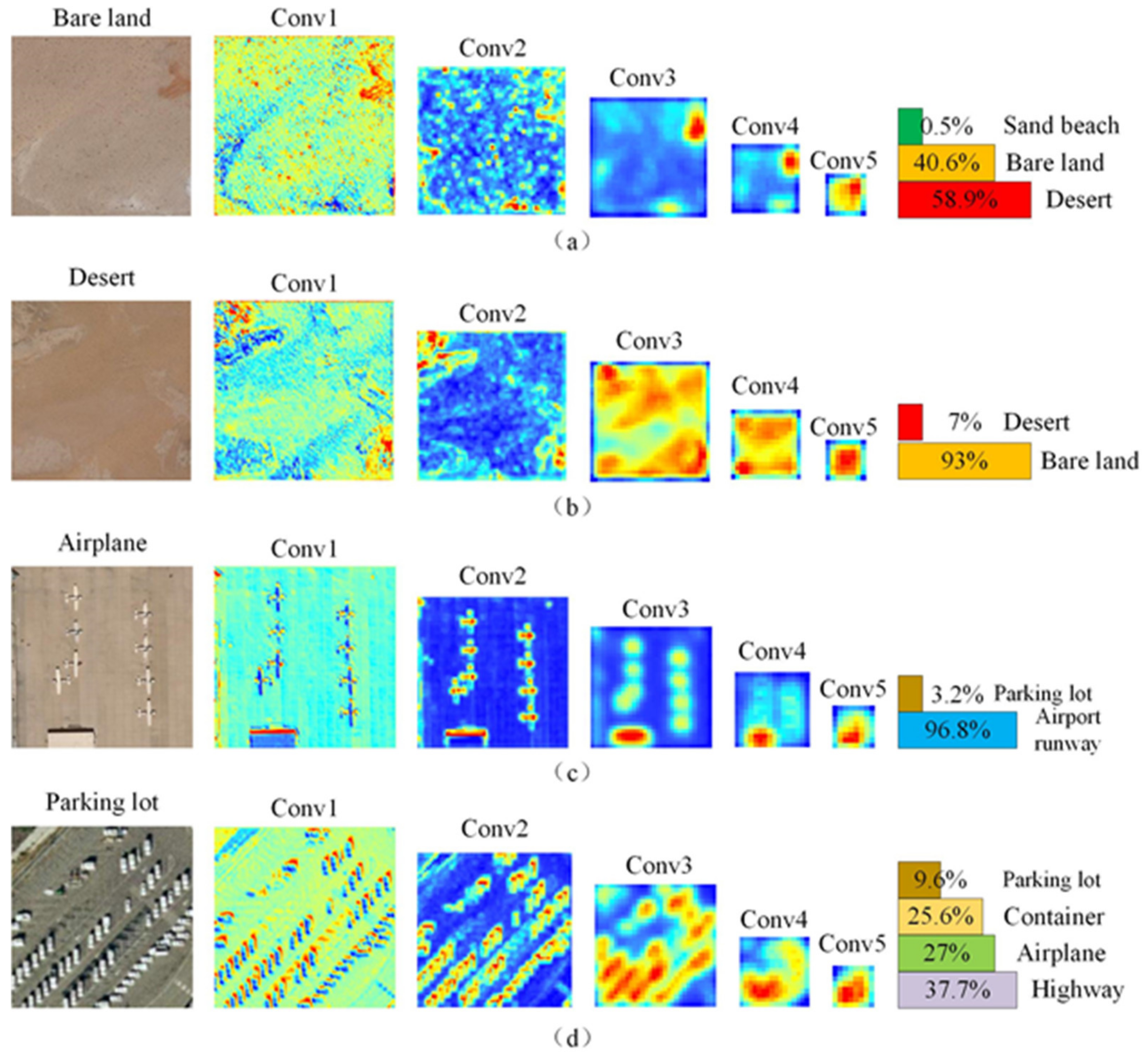
Although the proposed method performed well in feature extraction, there is some limitations in some aspects, such as the recognition of small and similar objects. As examples, Figure 16 presents the classification processes for some similar scenes. As can be seen from Figure 16a,b, bare land and desert display quite similar features in visual characteristics. The first two convolution layers extracted low-level texture and color features during feature extraction of these two scenes while the last three convolution layers synthesized the low-level features. Lastly, the fully connected layer identified the scene of the image with those features, and the classification with labels was completed. The high similarity of the extracted features as shown in Figure 16a,b caused confusion between these two scenes in the fully connected layers. For example, in Figure 16a, bare land is discriminated to be “desert” by the model with a probability of 58.9%. On the contrary, in Figure 16b, the desert is recognized as bare land. As can be seen in Figure 16c that the extracted background features in the scene of the airplane is very similar to that of the airport runway, and the airplanes in Figure 16c are small and therefore were mistakenly recognized as cars by the model, Figure 16c is thus categorized into airport runway and parking lot mistakenly. The extracted features as shown in Figure 16d were rather complicated that the first convolution layer accurately extracted those high-frequency signals; however, the model identified these high-frequency signals as airplanes or containers, and the background was identified as highways by mistake. From the above analysis, we can draw the conclusions as follows: (1) If two scenes both without high-frequency signals and the backgrounds of these two scenes are similar (as examples in Figure 16a,b), these two scenes would easily make the trained models confused to recognize the classes correctly; (2) although MGCNN-A is capable of extracting the small objects in the scene, it is yet difficult to label their categories correctly (as examples in Figure 16c,d).
5. Conclusions
In the present study, two grouped convolutional neural networks aimed for remotely sensed image scene classifications, namely, MGCNN and MGCNN-A developed on the basis of ResNet-50, were proposed and tested with RSI-CB and UC-Merced datasets. Firstly, data augmentation scheme was experimentally applied to three popularized convolutional neural networks, i.e., VGGNet-16, GoogLeNet-22, and ResNet-50, to investigate their performances in remotely sensed image scene classifications; the results strongly suggested the effectiveness of data augmentation in improving performance of classifications with these networks, and the ResNet-50 performed the best according to several criterions. To evaluate the performances of the proposed networks developed from ResNet-50 as backbone, several rigorously designed experiments were conducted with the proposed models by using RSI-CB and UC-Merced datasets to evaluate their performances. The experimental results indicated that grouping enabled the proposed models to learn more abundant features, therefore, benefiting the model in distinguishing different remotely sensed image scenes more effectively. Although MGCNN-A is not much better than MGCNN, it can be seen from the discussion that MGCNN-A is more robust in some categories. Although our proposed MGCNN and MGCNN-A models outperformed the similar ones comparably, some limitations yet remained in classification of some scenes with similar backgrounds but without high-frequency signals. Future attempts will be focused on adjusting our proposed models with feature fusion and transferring them into segmentation tasks.
Author Contributions
X.W. and Z.Z. designed this study. X.W. performed the data collection, model derivation, and validation with help from Z.Z. and Y.Y. The corresponding author W.Z. is supervisor of this work and contributed with continuous guidance during this work. X.W. and Z.Z. jointly wrote this manuscript, and the manuscript was edited by W.Z., Q.X., and C.Z. All authors have read and agreed to the published version of the manuscript.
Funding
This study was jointly financed by the National Key R & D Program of China [Grant No. 2016YFA0602302] and the Key R & D and Transformation Program of Qinghai Province [Grant No. 2020-SF-C37].
Institutional Review Board Statement
Not applicable.
Informed Consent Statement
Not applicable.
Data Availability Statement
The UC Merced Land Use Dataset in this study are openly and freely available at http://weegee.vision.ucmerced.edu/datasets/landuse.html. The RSI-CB Dataset in this study are openly and freely available at http://www.graphnetcloud.cn/1-10.
Acknowledgments
The authors are grateful to the anonymous reviewers for their constructive comments and suggestions to improve this manuscript; the graduate students in Wanchang Zhang’s group for open discussions in weekly seminars; and all the scholars for their reference researches.
Conflicts of Interest
The authors declare no conflict of interest.
References
- Zhao, H.; Zhang, Y.; Liu, S.; Shi, J. PSANet: Point-wise Spatial Attention Network for Scene Parsing. In Proceedings of the European Conference on Computer Vision, Munich, Germany, 8–14 September 2018; pp. 267–283. [Google Scholar] [CrossRef]
- Zhao, J.; Zhong, Y.; Shu, H.; Zhang, L. High-resolution image classification integrating spectral-spatial-location cues by conditional random fields. IEEE Trans. Image Process. 2016, 25, 4033–4045. [Google Scholar] [CrossRef]
- Yi, Y.; Zhang, Z.; Zhang, W.; Zhang, C.; Li, W.; Zhao, T. Semantic segmentation of urban buildings from VHR remote sensing imagery using a deep convolutional neural network. Remote Sens. 2019, 11, 1774. [Google Scholar] [CrossRef] [Green Version]
- Shawky, O.A.; Hagag, A.; El-Dahshan, E.S.A.; Ismail, M.A. Remote sensing image scene classification using CNN-MLP with data augmentation. Optik 2020, 221, 165356. [Google Scholar] [CrossRef]
- Zhang, R.; Chen, Z.; Zhang, S.; Song, F.; Zhang, G.; Zhou, Q.; Lei, T. Remote sensing image scene classification with noisy label distillation. Remote Sens. 2020, 12, 2376. [Google Scholar] [CrossRef]
- Xu, K.; Huang, H.; Deng, P.; Shi, G. Two-stream feature aggregation deep neural network for scene classification of remote sensing images. Inf. Sci. 2020, 539, 250–268. [Google Scholar] [CrossRef]
- Ma, A.; Wan, Y.; Zhong, Y.; Wang, J.; Zhang, L. SceneNet: Remote sensing scene classification deep learning network using multi-objective neural evolution architecture search. ISPRS J. Photogramm. Remote Sens. 2021, 172, 171–188. [Google Scholar] [CrossRef]
- Shi, S.; Chang, Y.; Wang, G.; Li, Z.; Hu, Y.; Liu, M.; Li, Y.; Li, B.; Zong, M.; Huang, W. Planning for the wetland restoration potential based on the viability of the seed bank and the land-use change trajectory in the Sanjiang Plain of China. Sci. Total Environ. 2020, 733, 139208. [Google Scholar] [CrossRef]
- Yi, Y.; Zhang, Z.; Zhang, W.; Jia, H.; Zhang, J. Landslide susceptibility mapping using multiscale sampling strategy and convolutional neural network: A case study in Jiuzhaigou region. Catena 2020, 195, 104851. [Google Scholar] [CrossRef]
- Jeong, D.; Kim, M.; Song, K.; Lee, J. Planning a Green Infrastructure Network to Integrate Potential Evacuation Routes and the Urban Green Space in a Coastal City: The Case Study of Haeundae District, Busan, South Korea. Sci. Total Environ. 2021, 761, 143179. [Google Scholar] [CrossRef] [PubMed]
- Zhang, D.; Pan, Y.; Zhang, J.; Hu, T.; Zhao, J.; Li, N.; Chen, Q. A generalized approach based on convolutional neural networks for large area cropland mapping at very high resolution. Remote Sens. Environ. 2020, 247, 111912. [Google Scholar] [CrossRef]
- Huang, B.; Zhao, B.; Song, Y. Urban land-use mapping using a deep convolutional neural network with high spatial resolution multispectral remote sensing imagery. Remote Sens. Environ. 2018, 214, 73–86. [Google Scholar] [CrossRef]
- Cao, S.; Du, M.; Zhao, W.; Hu, Y.; Mo, Y.; Chen, S.; Cai, Y.; Peng, Z.; Zhang, C. Multi-level monitoring of three-dimensional building changes for megacities: Trajectory, morphology, and landscape. ISPRS J. Photogramm. Remote Sens. 2020, 167, 54–70. [Google Scholar] [CrossRef]
- Mohammadi, H.; Samadzadegan, F. An object based framework for building change analysis using 2D and 3D information of high resolution satellite images. Adv. Space Res. 2020, 66, 1386–1404. [Google Scholar] [CrossRef]
- Mustaqeem; Kwon, S. CLSTM: Deep feature-based speech emotion recognition using the hierarchical convlstm network. Mathematics 2020, 8, 2133. [Google Scholar] [CrossRef]
- Lowe, D.G. Distinctive image features from scale-invariant keypoints. Int. J. Comput. Vis. 2004, 60, 91–110. [Google Scholar] [CrossRef]
- Philbin, J.; Chum, O.; Isard, M.; Sivic, J.; Zisserman, A. Object retrieval with large vocabularies and fast spatial matching. In Proceedings of the 2007 IEEE Conference on Computer Vision and Pattern Recognition, Minneapolis, MN, USA, 17–22 June 2007. [Google Scholar] [CrossRef]
- Krizhevsky, A.; Sutskever, I.; Hinton, G. Imagenet classification with deep convolutional neural networks. Adv. Neural Inf. Process. Syst. 2012, 25, 1097–1105. [Google Scholar] [CrossRef]
- Simonyan, K.; Zisserman, A. Very deep convolutional networks for large-scale image recognition. In Proceedings of the 3rd International Conference on Learning Representations, San Diego, CA, USA, 7–9 May 2015; pp. 1–14. [Google Scholar] [CrossRef]
- Szegedy, C.; Liu, W.; Jia, Y.; Sermanet, P.; Reed, S.; Anguelov, D.; Erhan, D.; Vanhoucke, V.; Rabinovich, A. Going deeper with convolutions. In Proceedings of the IEEE Conference on Computer Vision and Pattern Recognition, Boston, MA, USA, 7–12 June 2015; pp. 1–9. [Google Scholar] [CrossRef] [Green Version]
- He, K.; Zhang, X.; Ren, S.; Sun, J. Deep residual learning for image recognition. In Proceedings of the IEEE Conference on Computer Vision and Pattern Recognition, Las Vegas, NV, USA, 27–30 June 2016; pp. 770–778. [Google Scholar] [CrossRef] [Green Version]
- Huang, G.; Liu, Z.; Van Der Maaten, L.; Weinberger, K.Q. Densely connected convolutional networks. In Proceedings of the IEEE Conference on Computer Vision and Pattern Recognition, Honolulu, HI, USA, 21–26 July 2017; pp. 2261–2269. [Google Scholar] [CrossRef] [Green Version]
- Hu, J.; Shen, L.; Albanie, S.; Sun, G.; Wu, E. Squeeze-and-Excitation Networks. In Proceedings of the IEEE Conference on Computer Vision and Pattern Recognition, Salt Lake City, UT, USA, 18–23 June 2018; pp. 7132–7141. [Google Scholar] [CrossRef] [Green Version]
- Li, X.; Wang, W.; Hu, X.; Yang, J. Selective kernel networks. In Proceedings of the IEEE Conference on Computer Vision and Pattern Recognition, Long Beach, CA, USA, 15–20 June 2019; pp. 510–519. [Google Scholar] [CrossRef] [Green Version]
- Xie, S.; Girshick, R.; Dollár, P.; Tu, Z.; He, K. Aggregated residual transformations for deep neural networks. In Proceedings of the IEEE Conference on Computer Vision and Pattern Recognition, Honolulu, HI, USA, 21–26 July 2017; pp. 5987–5995. [Google Scholar] [CrossRef] [Green Version]
- Fu, K.; Chang, Z.; Zhang, Y.; Xu, G.; Zhang, K.; Sun, X. Rotation-aware and multi-scale convolutional neural network for object detection in remote sensing images. ISPRS J. Photogramm. Remote Sens. 2020, 161, 294–308. [Google Scholar] [CrossRef]
- Liu, T.; Yang, L.; Lunga, D. Change detection using deep learning approach with object-based image analysis. Remote Sens. Environ. 2021, 256, 112308. [Google Scholar] [CrossRef]
- Zhang, H.; Gong, M.; Zhang, P.; Su, L.; Shi, J. Feature-Level Change Detection Using Deep Representation and Feature Change Analysis for Multispectral Imagery. IEEE Geosci. Remote Sens. Lett. 2016, 13, 1666–1670. [Google Scholar] [CrossRef]
- Tuia, D.; Pasolli, E.; Emery, W.J. Using active learning to adapt remote sensing image classifiers. Remote Sens. Environ. 2011, 115, 2232–2242. [Google Scholar] [CrossRef]
- Bruzzone, L.; Fernández Prieto, D. A partially unsupervised cascade classifier for the analysis of multitemporal remote-sensing images. Pattern Recognit. Lett. 2002, 23, 1063–1071. [Google Scholar] [CrossRef] [Green Version]
- Han, X.; Zhong, Y.; Cao, L.; Zhang, L. Pre-trained alexnet architecture with pyramid pooling and supervision for high spatial resolution remote sensing image scene classification. Remote Sens. 2017, 9, 848. [Google Scholar] [CrossRef] [Green Version]
- Gong, X.; Xie, Z.; Liu, Y.; Shi, X.; Zheng, Z. Deep salient feature based anti-noise transfer network for scene classification of remote sensing imagery. Remote Sens. 2018, 10, 410. [Google Scholar] [CrossRef] [Green Version]
- Li, L.; Liang, P.; Ma, J.; Jiao, L.; Guo, X.; Liu, F.; Sun, C. A multiscale self-adaptive attention network for remote sensing scene classification. Remote Sens. 2020, 12, 2209. [Google Scholar] [CrossRef]
- Wang, Q.; Member, S.; Liu, S.; Chanussot, J. Scene Classification With Recurrent Attention of VHR Remote Sensing Images. IEEE Trans. Geosci. Remote Sens. 2019, 57, 1155–1167. [Google Scholar] [CrossRef]
- Mustaqeem; Kwon, S. MLT-DNet: Speech emotion recognition using 1D dilated CNN based on multi-learning trick approach. Expert Syst. Appl. 2021, 167, 114177. [Google Scholar] [CrossRef]
- Zhao, X.; Zhang, J.; Tian, J.; Zhuo, L.; Zhang, J. Residual dense network based on channel-spatial attention for the scene classification of a high-resolution remote sensing image. Remote Sens. 2020, 12, 1887. [Google Scholar] [CrossRef]
- Guo, D.; Xia, Y.; Luo, X. Scene Classification of Remote Sensing Images Based on Saliency Dual Attention Residual Network. IEEE Access 2020, 8, 6344–6357. [Google Scholar] [CrossRef]
- Chen, L.; Zhang, H.; Xiao, J.; Nie, L.; Shao, J.; Liu, W.; Chua, T.S. SCA-CNN: Spatial and channel-wise attention in convolutional networks for image captioning. In Proceedings of the IEEE Conference on Computer Vision and Pattern Recognition, Honolulu, HI, USA, 21–26 July 2017; pp. 6298–6306. [Google Scholar] [CrossRef] [Green Version]
- Mustaqeem; Kwon, S. Att-Net: Enhanced emotion recognition system using lightweight self-attention module. Appl. Soft Comput. 2021, 102, 107101. [Google Scholar] [CrossRef]
- Li, H.; Dou, X.; Tao, C.; Wu, Z.; Chen, J.; Peng, J.; Deng, M.; Zhao, L. Rsi-cb: A large-scale remote sensing image classification benchmark using crowdsourced data. Sensors 2020, 20, 1594. [Google Scholar] [CrossRef] [Green Version]
- Yang, Y.; Newsam, S. Bag-of-visual-words and spatial extensions for land-use classification. In Proceedings of the 18th SIGSPATIAL International Symposium on Advances in Geographic Information Systems, San Jose, CA, USA, 2–5 November 2010; pp. 270–279. [Google Scholar] [CrossRef]
- Fonał, K.; Zdunek, R. Fast hierarchical tucker decomposition with single-mode preservation and tensor subspace analysis for feature extraction from augmented multimodal data. Neurocomputing 2021, 445, 231–243. [Google Scholar] [CrossRef]
Figure 1.
Framework of model.

Figure 2.
Grouped convolution.

Figure 3.
Architecture of the channel attention block.

Figure 4.
Grouped attention block.

Figure 5.
Scheme diagram showing cross-validation used in the study.

Figure 6.
Sample images of each category in RSI-CB dataset: (1) airplane, (2) airport runway, (3) artificial grassland, (4) avenue, (5) bare land, (6) bridge, (7) city building, (8) coastline, (9) container, (10) crossroads, (11) dam, (12) desert, (13) dry farm, (14) forest, (15) green farmland, (16) highway, (17) hirst, (18) lake shore, (19) mangrove, (20) marina, (21) mountain, (22) parking lot, (23) pipeline, (24) residents, (25) river, (26) river protection forest, (27) sand beach, (28) sapling, (29) sea, (30) shrub wood, (31) snow mountain, (32) sparse forest, (33) storage room, (34) stream, (35) town.

Figure 7.
Sample images of each category in the UC-Merced Land Use dataset: (1) agricultural, (2) airplane, (3) baseball diamond, (4) beach, (5) buildings, (6) chaparral, (7) dense residential, (8) forest, (9) freeway, (10) golf course, (11) harbor, (12) intersection, (13) medium residential, (14) mobile home park, (15) overpass, (16) parking lot, (17) river, (18) runway, (19) sparse residential, (20) storage tanks, (21) tennis court.

Figure 8.
CM of ResNet-50 derived with the RSI-CB dataset.

Figure 9.
CM of MGCNN-C4 derived with the RSI-CB dataset.

Figure 10.
CM of MGCNN-A4 experimentally obtained with the RSI-CB dataset.

Figure 11.
CM of ResNet-50 obtained with the UC-Merced dataset.

Figure 12.
CM of MGCNN-C4 obtained with the UC-Merced dataset.

Figure 13.
CM of MGCNN-A4 obtained with the UC-Merced dataset.

Figure 14.
Faulty classified categories in the experiments. Figures (a–h) are the two same categories in RSI-CB and UC-Merced datasets.
Figure 14.
Faulty classified categories in the experiments. Figures (a–h) are the two same categories in RSI-CB and UC-Merced datasets.

Figure 15.
Feature maps extracted with the proposed models for comparisons. Figures (a–d) are feature maps of each group.
Figure 15.
Feature maps extracted with the proposed models for comparisons. Figures (a–d) are feature maps of each group.

Figure 16.
Examples of classification processes for some similar scenes with MGCNN-A. Figures (a–d) are the feature maps of convolution layers.
Figure 16.
Examples of classification processes for some similar scenes with MGCNN-A. Figures (a–d) are the feature maps of convolution layers.


Table 1.
The basic framework of the three models.
| Layers | ResNet-50 | MGCNN | MGCNN-A |
|---|---|---|---|
| Conv1 | 7 × 7, 64, stride 2 | 7 × 7, 64, stride 2 | 7 × 7, 64, stride 2 |
| Conv2 | 3 × 3 max pool, stride 2 | 3 × 3 max pool, stride 2 | 3 × 3 max pool, stride 2 |
| Conv3 | |||
| Conv4 | |||
| Conv5 | |||
| FC | Global average pool, FC, Softmax | Global average pool, FC, Softmax | Global average pool, FC, Softmax |
Table 2.
Comparisons of OA for base networks with and without data augmentation.
| Method | Overall Accuracy (%) | |
|---|---|---|
| Without Data Augmentation | With Data Augmentation | |
| VGGNet-16 | 81.831 | 89.849 |
| GoogLeNet-22 | 91.815 | 93.791 |
| ResNet-50 | 93.417 | 94.930 |
Table 3.
Overall accuracy (OA) of MGCNN.
| Method | Overall Accuracy (%) |
|---|---|
| ResNet-50 | 94.930 |
| MGCNN-C2 | 96.859 |
| MGCNN-C4 | 96.881 |
| MGCNN-C8 | 96.409 |
| MGCNN-C16 | 96.303 |
Table 4.
Overall accuracy (OA) of MGCNN-A.
| Method | Overall Accuracy (%) |
|---|---|
| ResNet-50 | 94.930 |
| MGCNN-A2 | 95.704 |
| MGCNN-A4 | 96.294 |
| MGCNN-A8 | 95.513 |
| MGCNN-A16 | 95.626 |
Table 5.
Overall accuracy (OA) of base networks with data augmentation.
| Method | Overall Accuracy (%) | |
|---|---|---|
| Without Data Augmentation | With Data Augmentation | |
| VGGNet-16 | 76.524 | 79.381 |
| GoogLeNet-22 | 77.810 | 85.286 |
| ResNet-50 | 81.524 | 88.857 |
Table 6.
Overall accuracy (OA) achieved by the MGCNN with UC-Merced dataset.
| Method | Overall Accuracy (%) |
|---|---|
| ResNet-50 | 88.857 |
| MGCNN-C2 | 91.190 |
| MGCNN-C4 | 91.905 |
| MGCNN-C8 | 91.096 |
| MGCNN-C16 | 90.143 |
Table 7.
Overall accuracy (OA) achieved by the MGCNN-A with UC-Merced dataset.
| Method | Overall Accuracy (%) |
|---|---|
| ResNet-50 | 88.857 |
| MGCNN-A2 | 90.286 |
| MGCNN-A4 | 91.524 |
| MGCNN-A8 | 90.667 |
| MGCNN-A16 | 90.429 |
Table 8.
Accuracy of two categories classified with three models.
| Model | Accuracy (%) | |
|---|---|---|
| Airplane | Parking Lot | |
| ResNet-50 | 82 | 87 |
| MGCNN-C4 | 84 | 92 |
| MGCNN-A4 | 86 | 95 |
Publisher’s Note: MDPI stays neutral with regard to jurisdictional claims in published maps and institutional affiliations. |
© 2021 by the authors. Licensee MDPI, Basel, Switzerland. This article is an open access article distributed under the terms and conditions of the Creative Commons Attribution (CC BY) license (https://creativecommons.org/licenses/by/4.0/).
Share and Cite
MDPI and ACS Style
Wu, X.; Zhang, Z.; Zhang, W.; Yi, Y.; Zhang, C.; Xu, Q. A Convolutional Neural Network Based on Grouping Structure for Scene Classification. Remote Sens. 2021, 13, 2457. https://0-doi-org.brum.beds.ac.uk/10.3390/rs13132457
AMA Style
Wu X, Zhang Z, Zhang W, Yi Y, Zhang C, Xu Q. A Convolutional Neural Network Based on Grouping Structure for Scene Classification. Remote Sensing. 2021; 13(13):2457. https://0-doi-org.brum.beds.ac.uk/10.3390/rs13132457
Chicago/Turabian StyleWu, Xuan, Zhijie Zhang, Wanchang Zhang, Yaning Yi, Chuanrong Zhang, and Qiang Xu. 2021. "A Convolutional Neural Network Based on Grouping Structure for Scene Classification" Remote Sensing 13, no. 13: 2457. https://0-doi-org.brum.beds.ac.uk/10.3390/rs13132457
Note that from the first issue of 2016, this journal uses article numbers instead of page numbers. See further details here.