
Feature Fusion Approach for Temporal Land Use Mapping in Complex Agricultural Areas

1
Henan Industrial Technology Academy of Spatio-Temporal Big Data, Henan University, Kaifeng 475004, China
2
College of Geography and Environmental Science, Henan University, Kaifeng 475004, China
3
Key Laboratory of Geospatial Technology for the Middle and Lower Yellow River Regions, Ministry of Education, Henan University, Kaifeng 475004, China
4
Henan Technology Innovation Center of Spatial-Temporal Big Data, Henan University, Kaifeng 475004, China
5
Key Research Institute of Yellow River Civilization and Sustainable Development, Ministry of Education, Henan University, Kaifeng 475004, China
*
Author to whom correspondence should be addressed.
Remote Sens. 2021, 13(13), 2517; https://0-doi-org.brum.beds.ac.uk/10.3390/rs13132517
Submission received: 11 May 2021
/
Revised: 8 June 2021
/
Accepted: 23 June 2021
/
Published: 27 June 2021
(This article belongs to the Special Issue Remote Sensing Applications in Vegetation Classification)
Abstract
:Accurate temporal land use mapping provides important and timely information for decision making for large-scale management of land and crop production. At present, temporal land cover and crop classifications within a study area have neglected the differences between subregions. In this paper, we propose a classification rule by integrating the terrain, time series characteristics, priority, and seasonality (TTPSR) with Sentinel-2 satellite imagery. Based on the time series of Normalized Difference Water Index (NDWI) and Vegetation Index (NDVI), a dynamic decision tree for forests, cultivation, urban, and water was created in Google Earth Engine (GEE) for each subregion to extract cultivated land. Then, with or without this cultivated land mask data, the original classification results for each subregion were completed based on composite image acquisition with five vegetation indices using Random Forest. During the post-reclassification process, a 4-bit coding rule based on terrain, type, seasonal rhythm, and priority was generated by analyzing the characteristics of the original results. Finally, statistical results and temporal mapping were processed. The results showed that feature importance was dominated by B2, NDWI, RENDVI, B11, and B12 over winter, and B11, B12, NDBI, B2, and B8A over summer. Meanwhile, the cultivated land mask improved the overall accuracy for multicategories (seven to eight and nine to 13 during winter and summer, respectively) in each subregion, with average ranges in the overall accuracy for winter and summer of 0.857–0.935 and 0.873–0.963, respectively, and kappa coefficients of 0.803–0.902 and 0.835–0.950, respectively. The analysis of the above results and the comparison with resampling plots identified various sources of error for classification accuracy, including spectral differences, degree of field fragmentation, and planting complexity. The results demonstrated the capability of the TTPSR rule in temporal land use mapping, especially with regard to complex crops classification and automated post-processing, thereby providing a viable option for large-scale land use mapping.
1. Introduction
The global COVID-19 pandemic, locust plagues, and extreme weather events in 2020 seriously destabilized global food security according to the United Nations Food and Agriculture Organization (UNFAO). Along with the International Panel on Climate Change (IPCC) report on “Climate Change and Land” [1], both agencies have stated that the restoration of agricultural land, adjustments to global agricultural production, and strengthening of global food supplies are essential to managing future food security issues. Cropping structures also have a further significant impact on land use and soil degradation. Therefore, accurately extracting regional crop planting structure timelines is the key to crop yield estimation, disaster mitigation, and responses to food crises, as well as responding to global environmental change and maintaining sustainable land use [2].
As an intuitive use of agricultural resources, information on crop planting structure involves the type, planting method, percentage, and spatial distribution of crops, dominated by food crops, and supplemented by other economic activities [3]. However, with increasing population pressure and food demand, crop planting structure becomes increasingly complex, including the combination of continuous cropping, rotation, inter-, and intra-cropping [4,5]. In 2018, Bégué et al. [6] mapped various complex crop rotation and fallow planting patterns in detail. Complex crop planting methods alleviate the food crisis to a certain extent, but also bring many challenges to ground-survey and landcover mapping [7]. Therefore, it is necessary to obtain timely and accurate information on crop planting structures and their spatio-temporal changes by using large-scale ground observation technology.
The unique monitoring capabilities of remote sensing science for spatial objects offers repetitive and effective data acquisition at large-scale spatial distributions, all of which are similarly essential for agricultural production management, sustainable development, and national food security [8,9]. China is a highly agricultural country, yet it is difficult to extract crop planting structures due to the high degrees of field fragmentation, complex planting methods, and differences in planting time and crop growth rates. Therefore, through the creation of crop classification and processing rules, which integrate the spectral characteristics of different crops, terrain, and seasonal characteristics, we can calculate the area and distribution of regional crop planting structures.
Monitoring agricultural conditions via remote sensing from global- to local-scales can provide a basis for the extraction of crop spectral signatures from imaging satellites, such as Sentinel-2, Landsat 8, and Gaofen-1 (GF-1) [10,11,12]. Several approaches have been devised to extract complex crop areas from Sentinel-2 imagery, especially red-edge-based methods [13] and hybrid methods that seek to address the phenology differences in one category from another [14], demonstrating how the availability of such imagery is beneficial to this domain. An attractive challenge in the remote sensing community is how to effectively combine the multiple features provided by geography and agronomy, such that they can be considered complementary with respect to the crop planting extraction mapping task in complex agricultural areas.
Since 1970, the United States and Europe have gradually begun to monitor large-area crops and yield estimates using remote sensing technology and China Crop Watch System with Remote Sensing, established by China in 1997. These technologies are of great significance to agricultural production management, sustainable development, and national food security [15]. However, a complex crop planting structure is more likely to produce mixed pixels in low- or medium-spatial resolution images, affecting crop classification accuracy. Therefore, in the application of satellite image classification for agricultural purposes, several researchers put forward a series of methods to obtain accurate crop information to serve agricultural production, such as single imagery with an optimal phenological period [16], fusion features (such as spectral characteristics, vegetation indices, texture, etc.) [17], time-series/multi-source satellite-image-based [18], and combining satellite images and statistical data [19].
Mathur et al. [20] used the IRS-1D image and SVM classifier approach to extract the spatial distribution of cotton and rice crops in Punjab, India, which reduced the total financial outlay in classification production and evaluation by ~26%. Chance et al. [21] achieved trend detection for irrigated agriculture in Idaho’s Snake River Plain for the time series of 1984–2016 Landsat-based at a 30 m resolution, which is critical for building strategies to support effective management of water resources in agricultural production. Several researchers have proposed time-series-based approach to classify different crops by using images with low- or medium- spatial resolution such as the Moderate Resolution Imaging Spectroradiometer (MODIS), Landsat or Sentinel-2 [5,22]. Consequently, it provides not only basic data for agricultural management at different regional scales, but also provides a method reference for temporal crop planting structure extraction in this study. In addition, remote sensing with high-resolutions, such as Worldview and unmanned aerial vehicles (UAVs), provides alternative techniques for monitoring heterogeneous crops in smallholder agriculture by object-oriented classification method [23,24]. Nevertheless, due to the difficult processing and lack of a red-edge band for complex crop extraction, it is difficult to apply these techniques in a large-area crop planting structure extraction. Therefore, according to the above researches, the medium-resolution image with the red-edge band is more effective in monitoring the complex agricultural crop planting structure by integrating vegetation indices, seasonal rhythm, and crop phenology.
For crop extraction, numerous approaches based on unsupervised and supervised classification techniques have been used to map geographic distributions and planting patterns. Currently, machine learning is defined as a scientific field that provides machines the ability to learn without being strictly programmed. Machine learning algorithms are used to identify different crops through single images [16], multi-temporal imagery [17], or fusion features [18]. The majority of the current research, however, focuses on the extraction of staple crops, and dynamic thresholds under variable terrains are rarely considered when building a decision tree [25]. Furthermore, these studies ignore the extraction of special crops across different regions, and accuracy is evaluated across the entire study area while neglecting the subregional-accuracy. For the regularization and automatic post-processing of classification results, seasonality is also often ignored. Furthermore, traditional methods, such as ERDAS Imagine, ENVI, and eCognition, lead to low efficiency large-area crop extraction owing to time-consuming processes, such as image data acquisition, preprocessing, and classification. All of these limitations highlight the need to develop more efficient and accurate methods to extract cropping structures.
With the advent of accessible satellite data, it is easier to create low-cost crop planting structure maps using features derived from remotely sensed spectral differences in vegetation and other surfaces over time [26]. These efforts have been aided by the success of object-oriented method and machine learning methods, such as support vector machines (SVM), random forests (RF), neural networks (NN) and deep learning (DL) [27], which allow for large-scale automated analysis of satellite imagery. For instance, membership probabilities of maximum likelihood classifier (MLC) [28], segmentation threshold of decision tree (DT) [29], or multilayer neural network [30] have been used on information extraction of multi-source images. The convenient data storage and cloud computing capabilities of the Google Earth Engine (GEE), as well as the freely-shared satellite imagery from the Landsat, MODIS, and Sentinel missions, in addition to other publicly available geospatial datasets, collectively provide the technical and data capabilities for the rapid extraction of agricultural planting structures [31,32].
Machine learning algorithms are an important component of supervised classification research, and similar studies have been carried out on land cover changes [33], cotton production [34], residential mapping [35], climate prediction [36], vegetation identification [37], and aquatic weeds [38]. Recently, non-parametric machine learning algorithms like RF or SVM can overcome the shortcomings of conventional classifiers like MLC since they are not constrained to assumptions like the parametric distributions of the input data [39]. Object-Based Image Analysis (OBIA) is the subdivision of an image into homogeneous regions through the grouping of pixels in accordance with determined criteria of homogeneity and heterogeneity, which considers the analysis of an “object in space” instead of a “pixel in space” [40]. A time series of Landsat TM/ETM+ images was acquired to generate the thematic map of sugarcane in Brazil based on OBIA, and the classification achieved an overall accuracy of 94% and a Kappa coefficient of 0.87 [41]. However, the segmentation scale is difficult to determine in complex crop structure extraction. SVM and RF are well-established machine learning techniques that have given promising accuracy in crop classification and have been shown to perform more accurately than other classifiers in crop classification [20,39]. Grabska et al. [42] and Waske and Benediktsson [43] concluded that SVM in the forest tree species (Sentinel-2 image) and landcover classification of multisensory datasets had higher classification accuracy when compared with MLC and DT. RF from Breiman [44] have successfully been applied for crop classification. Moreover, Pal [45] concluded that RF was more suitable for multivariate classification, and the training time is shorter in the case of nonlinear kernel than that of SVM.
The Random Forest (RF) is a more mature machine learning algorithm for the automatic extraction of features in remote sensing imagery [46]. In addition, it computes a feature importance score that can be used to select and reduce variables, and appears to be robust to high feature space dimensionality [44,45]. Li and Chen [47] concluded that RF had the best performance on multiple indicators out of five different machine learning algorithms, including neural network, decision tree, logistic regression, Naïve Baye and support vector machine; however, this method was based on mathematical theory and financial management activity, which did does not apply to multi-crop classifications in geographic space. Pareeth et al. [48] applied RF to classify land cover based on a time series of Landsat 8 imagery and achieved an overall accuracy (OA) of 87.2%, with a kappa coefficient of 0.85; however, this method included fewer categories (i.e., the number of extraction crops) and did not consider crop classification and the influence of terrain or seasonality. Son et al. [49] used multi-temporal Sentinel-2 imagery and field-based classification to successfully identify rice paddies in a small area of Taiwan. By analyzing the characteristic small size of rice fields and information on crop phenology, an approach for mapping rice-growing areas was developed at the field level using multi-temporal Sentinel-2 data. However, only the rice crop was extracted, along with difficulties in obtaining field level data over large; the small study area, single crop analysis, and excessive data processing times do not satisfy the requirements for extracting crop planting structures over large regions.
Presently, in temporal remote sensing, research studies based on vegetation index (VI) or time-series images are impressive [50,51]. Zhai et al. [52] developed the automated method based on satellite image time series to map the spatial distribution of three major crops (maize, rice, and soybean) in northeastern China. Wen et al. [53] propose the pre-constrained method integrating phenology-based vegetation indexes and RF for multi-year (2012–2016) mapping in regions with a complex planting structure, such as areas cultivating maize, wheat, and sunflower, indicating that the phenology-based approach was effective in improving the classification accuracy. Liu et al. [54] and Liu et al. [55] use RapidEye and Landsat images to extract the distribution of single-season (including corn, soybean, etc.) and across-season crops (wheat in winter, and rice, cotton, corn, orchard, water, and bare-land in summer), which proves the effectiveness of red-edge band and time-series Normalized Difference Vegetation Index (NDVI) in improving classification accuracy, respectively. The above studies completed the classification of complex crops at different regional scales but neglected the particularity of crop planting structure and accuracy among different subregions. However, there are few researches on the extraction of large-scale crop patterns across seasons in complex agricultural areas with 10 m-resolution mapping.
In this study, the Normalized Difference Water Index (NDWI) and Normalized Difference Vegetation Index (NDVI) time series for four land types (i.e., forest, cultivated land, urban areas, and water) were established for the study area using the GEE and Sentinel-2 imagery. In combination with a digital elevation model (DEM), priority for reclassification processing, seasonality, and other information, a decision tree and post-processing reclassification rule were constructed. Based on these results, the land cover and crop planting structures for the entirety study area were extracted. Finally, the feature importance, overall accuracy, and influential factors for the derived land mask and extraction results over time were analyzed in detail. Our method can extract the crop planting structure via the fusion of multiple features, such as the terrain, time series characteristics, priority, and seasonality (TTPSR), when using a 10 m composite Sentinel-2 image covering the study area in Henan Province, China. The purpose of this study is to provide a new set of methods and rules for the automated processing of crop structures across complex large-scale agricultural areas, as well as to establish a reference for regional to national crop extraction.
2. Data and Study Sites
2.1. Study Sites
Henan Province, located in central China (31°23′N–36°22′N, 110°21′E–116°39′E), has a total area of ~165,000 km2 (Figure 1). Henan Province is classified as a monsoonal climate, extending from the northern subtropical to the warm temperate zone. The average annual temperature is between 10 and 17 °C, annual precipitation is between 407 and 1230 mm, and the frost-free period is >200 days. The corresponding periods of rain and heat are advantageous for cultivation. Crops within this study area are diverse and account for nearly 10% of the total grain production in China [56,57]. The terrain of the study area is highly variable with high elevations in the west and low elevations in the east, surrounded by mountains in the north, west, and south that gradually flatten out into hills, basins, and plains. The distribution of terrain is complex, and the degree of field fragmentation is particularly high in the mountainous and hilly areas. According to the 30 m DEM and terrain classification standard, the study area can be divided into three types: plains (<200 m), hills (≥200 m), and mountains (≥500 m; Figure 1b).
2.2. Dataset and Preprocessing
2.2.1. Sentinel-2 Data
With the launch of the Sentinel-2A and -2B satellites in 2015 and 2017, respectively, Sentinel-2, developed by the European Space Agency (ESA), comprises a constellation of two polar-orbiting satellites in the same sun-synchronous orbit, providing imagery across 13 spectral bands, with a 10-day revisit period and a maximum spatial resolution of 10 m (Table 1). Sentinel-2 has four red-edge bands (B5, B6, B7, and B8A), which provide important data for complex crop classification. B5 and B6 are particularly useful for red-edge position, B7 for calculating the inversion of the leaf area index (LAI) [58], and B8A is sensitive to LAI, chlorophyll, and biomass [59]. The data have been widely used in agricultural monitoring [60], ecological assessments [61], and land cover change analyses [62]. This study utilized the GEE to obtain Sentinel-2 archived data, as well as a quality band (QA60) that can be used for cloud masking to reduce the influence of noise on feature extraction. The Sentinel 2 satellite utilizes the Universal Transverse Mercator projection and follows the US-MGRS (U.S. Military Grid Reference System) to set the satellite orbit number; the number of images covering the study area ranged from (49SD–50SM) to (50RK–50SL). In addition, the three bands with a 60 m resolution (i.e., B1, B9, and B10) were removed during the classification process.
2.2.2. Crop Phenology
In Henan Province, the main rotation structures are between wheat and maize (two primary crops per year), and the main growth periods are shown in Figure 2. Winter crops (primarily wheat) are generally sown in early October, enter a jointing stage in March of the following year; following a growing stage, these crops mature and are harvested at the end of May. Spring crops, such as maize (MAI) and peanuts (PEA), are usually sown in early May, enter their peak growth period in mid-June, and are harvested in mid- to late-August. Tobacco (TOB) is considered a summer crop because it is grown only once a year and harvested in late-August. Summer crops (primarily maize) are generally sown in early June, enter a growing phase in mid-July, and are harvested in mid-September. When selecting imagery, considering the specific phenological periods of crops across seasons is important, as well as limiting the time intervals between images as much as possible.
In the early stages of crop growth, spectral information is largely uninformative owing to low crop coverage and a large relative influence from the ground surface [63]. Spectral information increases with growth and coverage, enabling crop identification. Accordingly, images from late February to early May were selected for winter crop classification while images from late July to early September were selected for summer crops. The planting area of crops in spring is small and relatively concentrated. To reduce the time and workload of classification, images are selected according to the over-lap time period of spring and summer, and distinguish whether it is a spring crop from the following two strategies. The first strategy is that if the winter-extraction is non-cultivated land, it can be determined that the crops are planted in spring. The other strategy is that if the image-feature is non-cultivated land in late-August or early-September, which indicates that the spring crops have been harvested, then the images from mid-June to late-July should be reselected for spring crop extraction. With cloud cover less than 10% in 2020, we obtained 346 and 153 images from 1 March to 18 May (for winter analysis) and from 1 August to 10 September (spring–summer analysis), respectively.
2.2.3. Sample Data
An accurate spectral characteristic of different crops in remote sensing images is essential for crop extraction. We use the ArcMap 10.5 in Getac F110 computer and Geomapper software in handheld GPS named Jisibao to obtain ground data, which can load and process image and vector data, and completely match the location information between the ground-data point and image. The Getac F110 is a GPS-equipped tablet with positioning accuracy <3 m. The GPS toolbox can provide a spatial-positioning module embedded in ArcMap, with location services for ground surveys. In order to distinguish the spectral characteristics of different ground objects, the difference was recorded in detail with more than ten kinds of bands-based false color composite, such as B8A/B11/B3, B8A/B4/B3, B6/B4/B1, B4/B3/B2 and so on. Based on this, the interpretation marks library is established as a reference for the next manual selection of sample data. The ground survey (Table 2) consisted of identifying precise locations via handheld GPS devices during crop growth phases to pair the crop type with the coordinate positions across different locations. The spatial distribution of the sample plots and points is shown in Figure 1a; notably, the ground survey of the spring and summer crops was carried out simultaneously. When collecting sample points on the ground, the location was ensured to be >5 m from the field boundary, and the total field area was greater than the area of three pixels in the imagery (30 m × 30 m). Based on this, the sample points and image pixels corresponding to ground objects can be matched, and the influence of mixed pixels can be reduced. The crop planting structure in summer is more complex than that in winter: a total of 2254 sample points were collected, 508 in winter and 1746 in summer. Planting structures in the individual fields of 115 sample plots (~500 × 500 m) were recorded in the same locations for winter and summer, with a total area of 2.51 km2.
Among all the sample plots, only the urban area remained unchanged (Table 2); the area of water cover changed in the summer due to the planting of lotus and other crops while the forested land area changed owing to interplanting of PEA and soybeans (SOY). Combined with the spectral characteristics of the ground survey data across different seasons and Tobler’s First Law of Geography [64], the number of samples, including both the ground survey and visually interpreted data, was increased to 35,592 and 44,828 based on different bands combination in the winter and summer, respectively. During the classification process, samples of each subregional unit were randomly split into training (70%) and testing (30%) subsets. The classification codes in Table 2 were used for crop classification in the GEE; the abbreviations were used to classify the different land type mapping analyses. According to the ground survey results, the major winter crops/coverage types were wheat (WHE), garlic (GAR), rapeseed (RAP), and non-cultivated (WNC) land; summer crops were dominated by maize, peanuts, soybeans, rice (RIC), tobacco, millet (MIL), sesame (SES), rehmannia (REH), and other vegetables or crops (SOTH). The staple and minor crop are relative in different subregions, which is the major crop in one subregion while being minor in another subregion. In addition, different crop planting structures expressed notable regional aggregation characteristics; therefore, this study used the municipal administrative divisions with relatively homogeneous internal planting structures as the subregional unit.
Different bands contain different spectral information, and their combination can reveal a unique spectral signature for certain features [65]. The images with Tile Number T50SKE and land types for the sample plots in the winter (17 April 2020) and summer (4 September 2020) are shown in Figure 3. The optimization selection R/G/B of images in winter and summer were B8A/B4/B3 and B8A/B11/B4, respectively. The true color composite is a widely used Earth observation product for displaying satellite imagery. However, the false color composite of different bands can highlight different features, especially the red edge band for complex crops. Combined with the ground survey data, we attempted to achieve visual interpretation of crops in different seasons with a variety of different false color synthetic bands. The spectral features reflected by the ground survey data in different band combinations (including B8A/B4/B3, B8A/B11/B3, B8/B11/B3, B4/B3/B2, and others) were recorded and utilized, and the sample points were selected by visual interpretation combined with the spatial position and shape of the image.
3. Methods
3.1. Overall Workflow
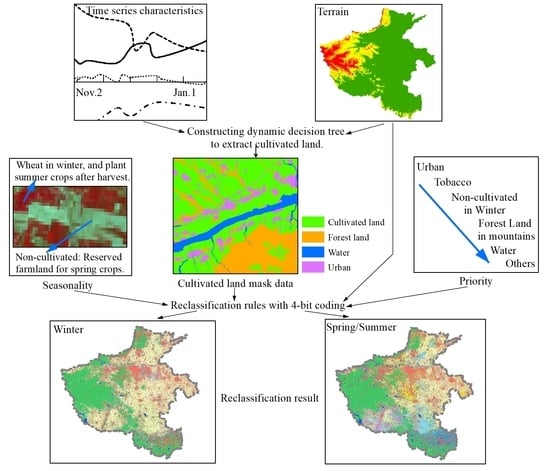
As shown in Figure 4, the overall workflow includes three stages: data processing, decision tree and classification, and reclassification and accuracy analyses. First, data processing included both ground survey data and image preprocessing. Second, NDWI and NDVI time series data were calculated for four landcover types (cultivated land, forest, water, and urban) based on the selected ground sample points, which were used to set the preliminary thresholds of a decision tree [66]. Then, a dynamic decision tree was created, combining the terrain and cultivated land areas in each subregional unit. The extraction results with and without masked cultivated land were classified based on the RF classifier. Finally, the RF extraction results for both seasons were processed using the reclassification rules, which were generated according to the terrain, seasonality, priority, and planting methods, such as interplanting. Feature importance and classification accuracy under different conditions were analyzed, and a single map of the crop planting structures with different fields in an attribute table through time was created for the study area. Overall, the TTPSR was constructed by multiple features, including the terrain, time series characteristics, priority, and seasonality.
3.2. Time Series Feature Analysis and Dynamic Decision Tree Construction
Landcover types (cultivated land, forest land, water, and urban) were extracted and masked to reduce the influence of non-agricultural regions on agricultural structure extraction. The preliminary decision tree was created through the following process.
First, 50 sample points for each landcover type were selected in the study area. Forest samples were mainly selected in mountainous and hilly regions, areas of perennial crop growth were selected for cultivated land, buildings and roads were selected for urban cover, and rivers and reservoirs were used for water.
Second, the time series of the NDWI and NDVI for selected sample sites in each landcover type were calculated (Figure 5a,b) using Sentinel-2 images (2556 images from 1 October 2019, to 30 September 2020); the doySeriesByRegion in the GEE and initial threshold values incorporated the seasonal variability in the vegetation indices. Discriminating between water and other landcover types was relatively straightforward (Figure 5a,b); an NDWI > 0.1 threshold was used to mask water pixels. Forests and cultivated land can be remotely distinguished from each other during the following three stages (Figure 5b): late September to mid-November (first stage), February to March (second stage), and late May to mid-June (third stage). Combined with the ground survey data, the first stage was marked by a rapid decrease in the NDVI for cultivated land caused by the bare surface following crop harvest; the NDVI for forested land also decreased slightly, but enough vegetation coverage was maintained to display a notable difference between the two landcover types. In the second stage, distinguishing parts of the forest from winter crops was difficult due to the high vegetation index values for evergreen forests in the southwest region. During the third stage, large areas of vegetable cultivation in central and eastern Henan Province during crop rotation are indistinguishable from forested land; therefore, the first stage NDVI was selected to distinguish between forests, cultivated land, urban, and water.
Preliminary decision tree classification rules were established based on the above analyses. In addition to the extraction threshold of water defined above (NDWI > 0.1), forested land was defined as NDVI ≥ 0.45 from 20 September to 1 November, cultivated land was defined as 0.03 ≤ NDVI < 0.45, and urban–water were considered as NDVI < 0.03. Urban pixels were extracted by masking these results with the water NDWI results.
We randomly generated 1000 sample points in the cultivated land mask data, and verified the accuracy of cultivated land classification based on the high-resolution image of Google Earth. The result shows that there are 972 cultivated land sample points and 28 non-cultivated land sample points (most of which are intercropping under forest and garden land). The accuracy of cultivated land extraction is 97.2%, which can meet the requirements of the crop extraction.
According to the terrain and spectral influence between different land types in each subregional unit, we found that forested land had a greater influence on cultivated land in hilly and mountainous regions, and the upper threshold limit of the decision tree was adjusted accordingly. In the plains, the spectra of staple crops had a significant influence on minor crops (such as garlic and other crops, such as onion), while decreased interference was observed between the agriculture and non-cultivated land. Therefore, according to the initially established decision tree and above analyses, the NDVI-based threshold between cultivated and non-cultivated areas was determined to be 0.01. Based on the premise of the maximum area of cultivated land in each basin unit, a threshold for the dynamic decision tree between forests and cultivated land was also established. The terrain area and thresholds for each subregional unit, as well as imagery dates, are listed in Table 3. Notably, obtaining imagery in the early period of summer cropping was difficult due to the influence of seasonal rain and clouds; hence, a portion of the images was selected in the later stages of crop growth. The threshold between forests and cultivated land in more mountainous areas was higher than those in the plains; therefore, when building the decision tree rules for different landcover types, factors, such as regional terrain and seasonality, were considered.
3.3. Classification Algorithm and Evaluation Indicators
RF is a machine learning algorithm built upon a classification and regression tree (CART) using the ensemble method developed by Breiman [44,67]. The algorithm utilizes bootstrap aggregation (i.e., bagging) to reduce overfitting and improve the generalization accuracy. The RF algorithm provides the feature importance assessed using the out-of-bag data samples [68], which has been used extensively to accurately classify various types of remote sensing imagery, such as the classification of glacial or non-glacial lakes [69] and for phenology-based crop type (sugar beets and grains) mapping [70].
The parameters of the RF classifier in the GEE were set to: numberOfTrees = 100; minLeafPopulation = 1, and the remaining parameters were left as their default values. The image acquisition dates and times of 15 characteristic bands for each subregional unit are listed in Table 3. The OA derived from the confusion matrix and kappa coefficient has been widely used in the literature for evaluation purposes; a detailed description of the methods can be found in Congalton [71]. As the training and test samples were split randomly, the classification results of each landcover type were repeated five times, and the average value was taken as the final value of the evaluation indicators, including the feature importance, OA, and kappa coefficients. Additionally, the reclassification accuracy was analyzed again with a combination of resampling plots and visual interpretation.
A raster of the resampling plots was used to ensure the consistency of the extraction results during the accuracy assessment while visual evaluations provided a direct method for analyzing the classification results. To assess the differences of seasonality, the feature importance of each classification result was normalized based on the maximum value; then, the average values of the feature importance for all subregional units with and without the cultivated land mask were calculated. The average of any feature, F, was computed as follows:
where for any subregional unit, Fi is the average feature importance of the ith feature repeated five times, Fi-max is the maximum value of all Fi, and n is the total number of subregional units.
3.4. Feature Band Establishment and Importance Assessment
Satellite imagery can be used to obtain spatially distributed reflectance data on plant growth and development at different stages of the growing season [72]. Vegetation indices are often used as parameters to evaluate the growth of vegetation and improve the classification accuracy of crops; however, the identification of texture features is difficult due to the limitations of an image’s spatial resolution, small field area, and complex crop types. Therefore, 15 feature bands, including 10 spectral bands and five vegetation indices, were generated for crop classification in each subregional unit. The five vegetation indices examined were NDVI, NDWI, Normalized Differences Built-up Index (NDBI), Red Edge NDVI (RENDVI), and Enhanced Vegetation Index (EVI), computed with Equations (2)–(6), respectively, as follows:
where B2, B3, B4, B5, B8, and B11 correspond to the bands of Sentinel-2, as listed in Table 1.
Figure 6 shows how the features are significantly affected by the spectral information for different land types in different seasons. The top five feature importance average values were winter with cultivated land mask (W_mask)—B2, NDWI, RENDVI, B11, and B12; winter without a cultivated land mask (W_nomask)—B2, NDWI, RENDVI, NDBI, and B11; and summer with (S_mask) and without cultivated land mask (S_nomask)—B11, B12, NDBI, B2, and B8A. Ultimately, feature importance was affected by the difference in seasonal land types. B2 and B11 are of high importance in the classification process across both seasons. In winter, NDWI and RENDVI were more important than the other vegetation indices; however, both were calculated using B3, B4 and B5, thus reflecting that among red-edge bands, B5 is of greater importance in winter crop classification (i.e., B5 > B6 > B8A > B7). In summer, NDBI is the most important vegetation index, and the feature importance of B8A was higher than that of the other red-edge bands. In conclusion, both the blue bands and shortwave infrared spectral bands had the highest importance values while the importance of the red-edge bands varied seasonally across land types, consistent with the conclusions of Song et al. [13].
3.5. Reclassification by Fusion of Seasonal and Multiple Features
The results of the pixel-based supervised classification almost always produce numerous scattered tiny spots known as the “salt and pepper” phenomenon. To minimize this effect and improve the accuracy, the RF extraction results with the cultivated land mask were calculated according to the reclassification rules, which fused the terrain, land types, priority, and seasonality. All reclassification processing and statistics were programmed in Python 2.7 and Arcpy; the main process was as follows:
1. DEM resampling: The 30 m DEM in the study area was resampled to a resolution consistent with the extraction results (10 × 10 m), and the terrain (plains, hills, and mountains) was reclassified as 1, 2 and 3, respectively (Tresult).
2. Extraction results for each subregional unit: The existence of zero values in the extraction results was caused by the maximum outer boundary of each subregion unit. Therefore, a function named SetNull was used to treat zero values as null and resave the results for winter and summer, termed Wresult and Sresult, respectively.
3. Priority analysis of land types: The difference in the spectral characteristics of similar land types lead to an inconsistency in the classification results for grassland and green areas at highway medians in urban areas. Therefore, the combined dataset for the urban extraction results for both seasons, and the union results for urban and rural residential areas were used (Figure 7). The extraction results for winter-based unplanted areas (WNC) and summer-based tobacco (TOB) had greater accuracy due to the small area and relatively simple planting structure of cultivated land in mountainous areas; hence, the original extraction results were largely maintained. There were inconsistencies, however, with mountainous forested land (MFL), especially in deciduous forest regions (e.g., shrublands); hence, the resulting MFL was a union of both seasonal datasets. Finally, in each season, both hilly and plains regions had crops planted under the forest canopy, and water areas (WAT) had different seasonal flood patterns and crop planting structures, such that the original extraction results were maintained. Therefore, the priority for different land types was URB > TOB or WNC > MFL > WAT > Other classification results.
4. Coding rule establishment: Combining Tresult, Sresult, and Wresult, a new 4-bit coding (TSSW) raster data (Calresult) was generated using the Raster Calculation in Arcpy and Equation (7):
As there were 14 categories in the summer extraction system, Calresult was set to a 4-bit code. When Wresult was WNC, MAI and PEA in the summer crops were reclassified as spring MAI and PEA.
5. Recoding and reclassification: The terrain code (Tcode), winter reclassification code (Wcode), summer reclassification code (Scode), and spring result code (Spcode) were automatically added and calculated based on the Calresult of each subregional unit. Then, according to the land type priority from Step (3), a single map of the reclassification results with different fields in the attribute table was generated. When SS = 06, or W = 6 in TSSW, the reclassification code for different seasons was 6-URB. A TSSW value of 3114 indicated that Tcode was 3-mountain, Wcode was 4-WNC, and Scode was 11-MAI; however, as Wcode was 4-WNC, Spcode should be 411-spring MAI; otherwise, Spcode is 11-MAI. All specific codes and land type abbreviations are listed in Table 2.
6. Filtering and result statistics: The nearest neighbor rule and a replacement threshold of “half” in the MajorityFilter tool were adopted to reduce noise by reclassifying tiny spots resulting from Step (5) into an adjacent large category to obtain the final classification result for each subregional unit. Finally, the area results for each were calculated using ZonalStatisticsStable tool.
4. Results and Analysis
4.1. Accuracy Assessment Analyses
4.1.1. Overall Accuracy
Accuracy analyses were carried out to test the performance of the RF algorithm under different conditions. Based on the same randomly generated training and testing datasets, Figure 8 shows the results of the five simulations for each subregional unit with and without the cultivated land mask across both seasons. In addition, the range of the Y-axis is set from 0.7 to 1 to compare the assessment indicators in the uniform range, with the following conclusions.
1. The OA and kappa coefficients of the extracted results in both seasons showed strong performances with RF compared with the sample point data. For all basic subregions, nearly 80% maintained an average OA > 0.85, and only two observed kappa coefficients were <0.8, i.e., Puyang City (0.770) and Shangqiu City (0.782), when assessed without the cultivated land mask in winter. With or without the cultivated land mask, the OA ranges in winter were 0.857–0.935 and 0.829–0.923 and the kappa coefficients were 0.803–0.902 and 0.770–0.891, respectively. Summer OA ranges observed with and without the land mask were 0.873–0.963 and 0.860–0.955 and the kappa coefficients were 0.835–0.950 and 0.817–0.940, respectively.
2. The extraction accuracy of each sample pixel with the agricultural land mask was significantly higher than that without the cultivated land mask, consistent with the conclusions of Forkuor et al. [73]. Comparing the average OA for the different seasons, there were eight subregional units with an increase of more than 2%.
3. The accuracy in summer was higher than that in winter, and the number of extracted categories were also greater. When sample points for the winter were selected, there was an apparent phenomenon of foreign bodies with similar spectral characteristics among sapling forests, unplanted cultivated land, construction sites, plastic mulching areas, and greenhouses, thereby making these objects difficult to distinguish. Although the number of extracted categories in summer was greater, the spectral characteristics among the land types were more varied and relatively easier to distinguish. Thus, consistent with the conclusions of Lim et al. [74] and Shao and Lunetta [75], the classification accuracies were directly related to the sample homogeneity/heterogeneity.
4. When examining the estimated spatial distribution of the results (Figure 9a,b), the OA of the staple crops maintaining a large proportion of the area was higher than the accuracy of minor crops, consistent with the findings of Liu et al. [55]. There were some misclassifications and incorrect classifications of minor crops. Therefore, the distribution of minor and other crops with varied spectral characteristics also affected the OA.
5. The accuracy indices for the cities of Sanmenxia and Xinyang both indicated relatively low precision results, which was likely attributable to the terrain and high degree of field fragmentation. Sanmenxia is located on the Loess Plateau, where mountains and hills account for 86.38% and 13.61% of the total area, respectively (i.e., 0% plains; Table 3). In addition, the highly fragmented field plots, complex land types, and difficulty in obtaining ground survey data were the primary drivers of the observed low OA. Xinyang is located in southern Henan Province, where plains account for 86.72%; however, the field boundary structures are irregular and complex (Figure 9c,d), and spectral features among different land types interfere with each other, decreasing the OA. In conclusion, terrain factors and complex field boundary structures had a significant influence on the observed OA.
The aim of the analyses of the evaluation indicators was to identify the factors affecting the extraction accuracy of crop structuring under different conditions. We note that the number of classification targets did not significantly contribute to the observed OA. Furthermore, the OA was improved by the cultivated land mask while factors, such as the separation results of different ground objects, minor crops and other crops, interaction of spectral information among different land types, terrain factors, field boundary structures, and the complexity of crop planting methods, all had major impacts on crop identification. Therefore, future should focus on analyzing and discriminating between the seasonality of crop structuring, as well as the seasonal characteristics and differences of ground objects, to further improve the classification accuracy in complex agricultural areas.
4.1.2. Comparison Analysis of Resampling Plots
The calculation of accuracy assessments based on field sample data is common practice; however, this approach may be unsuitable due to the complex topographical relationship between points and patches, in addition to the potential subjective bias in the spatial location selection of sample points [76]. Thus, we calculated the number of pixels within each land type, both in the resampling plots and the reclassification results, for winter and summer (Table 4), as well as the spatial distribution of different results for individual samples (Figure 10).
The reclassification accuracy of staple crops, such as WHE, MAI, PEA, RIC, and RAP, was superior to that of minor and other crops. In winter, WNC had a higher extraction accuracy due to a greater areal extent and distinct spectral characteristics, but it remained difficult to distinguish from URB coverage. With the spectral influence of WHE, the path of wheat fields was incorrectly classified as GAR (Figure 10b), driving the observed increase in GAR. The estimated areas of winter forests (WFL) and URB land were more than that of the resampling plots due to the spectral influence of roadside trees, and the spatial resolution of the images lead to the area of winter WHE in this region largely being classified as WFL. Additionally, greenhouses in the cultivated land, and some unplanted land were mistaken for URB. Except for GAR and RAP, other winter crops (WOTH) had relatively small areas and lacked contrast, such that their accuracy was not evaluated here. These were the main drivers for the observed inaccuracies between GAR and field roads, and WHE and WFL, as well as WNC and URB in winter.
In summer, crops, such as PEA, MAI, SOY, and RIC, all had a similar spectral influence as WHE. As SOY fields were relatively scattered and small, its boundaries were difficult to extract owing to the spectral interference of other crops. RIC was concentrated in the southern region of the study area, characterized by complex land types, irregular field boundary structures, and strong terrain changes (Figure 9c,d and Figure 11). These factors negatively influenced the classification accuracy of RIC, and were likely responsible for the difficulty in extracting the field boundaries for this region. Meanwhile, the driving factors for the observed overestimation of other crops were the more complex spectral characteristics from complex and fragmented fields, in addition to the variability in the harvest time for vegetables, sorghum, sweet potatoes, and medicinal plants, among others. In addition, an imbalance in the training samples lead to a considerably decreased amount of ground data for some categories, such as REH, SOTH, or summer unplanted areas (SNC), often resulting in the observed poor accuracy for these minority classes. Moreover, ground samples within the mountains were limited due to logistical and safety concerns. According to the visual interpretation of the sample points and reclassification results (Figure 11), SFL was the main landcover type observed in mountainous areas and had a high classification accuracy based on visual interpretation. Through an analysis of the pixel numbers in both sets of results, we found that the causes of the observed inaccuracy in crop classifications were similar to the drivers of the OA; however, the inconsistency between the regular spatial arrangement of the raster data, as well as the directions of the actual planting structures, also limited the spatial overlap between pixel and vector boundaries (Figure 10), a further driver of the observed classification inaccuracies.
Compared with the pixel numbers of the resampling plots, the extraction results of the staple crop areas were underestimated. In addition to variable terrain, field boundaries, planting structures, and mixed pixels, some classification errors were also caused by the difference between ground field boundaries and image arrangements. To improve the classification performance, appropriate resampling techniques or time series data should be the focus of future research.
4.2. Reclassification of Multi-Temporal Crop Planting Structure
The TTPSR-based approach was tested in Henan Province, and the multi-season 2020 crop planting structures at 10 m resolution were extracted. The total area represented by all land types was 165,325.18 km2, as calculated from the total extraction area of each subregional unit in Figure 11. The proportion of each land type in both seasons is listed in Table 5 and the spatial distribution results are shown in Figure 12i,ii. The proportion of SFL was higher than WFL as deciduous forests dominate the study area, in addition to the incorrect classification of young forest where vegetation fails to cover the ground surface, which can readily be mistaken for WNC from the high ground visibility. In addition, for WHE grown under deciduous forest canopies in the plains, its spectral pattern dominates from April to May, and can readily be classified using medium resolution imagery. Further, summer water areas were slightly higher than in the winter from seasonal changes in the climate and precipitation. Precipitation is mainly concentrated from June to August, flooding rivers and ponds. Compared with the summer reclassification results, the area of WFL and winter WAT decreased by 3.22% and 0.31%, respectively.
When comparing the results to crop areas from 2018 [57] (Table 5), the observed difference in the results was partly due to a lag in response to relevant provincial policies increasing the planting areas of more economically beneficial crops (e.g., peanuts), which has been observed in recent years. Combined with the visual interpretation, ground survey records, and the underestimated reclassification area of staple crops compared to actual planting areas in the resampling plots (see Section 4.1.2), the multi-seasonal reclassification results were largely consistent with the actual spatial distribution of crops in Henan Province, ultimately supporting the processing ability of TTPSR, as well as the extraction ability of complex crops and planting structures.
Based on Figure 12 and Table 5, forests are primarily distributed in the mountainous and hilly areas of northeastern, western, and southern Henan Province while the plains forests are mainly concentrated in southeastern Xuchang (Yanling County) and southern Xinyang (Huangchuan County). WAT coverage is mainly distributed in Nanyang and Xinyang. Urban areas account for 22.95% of the total area. WHE was the most widely planted crop, accounting for 32.22% of the total area, followed by MAI (22.02%). In winter, GAR was mainly planted in eastern Zhengzhou (Zhongmu County) and Kaifeng, and RAP was planted sporadically in southern Zhumadian and Xinyang. There were many unplanted paddies in Xinyang, which are difficult to sow due to standing field water after harvest. Unplanted land was relatively scattered, but primarily concentrated in the transitional mountainous and hilly areas in the cities of Sanmenxia and Luoyang, as well as to the west of Xuchang and the Nanyang Basin, areas mostly used for planting TOB and PEA in the spring. All other crops not analyzed individually were planted in smaller dispersed fields.
In the summer, planting areas for PEA, SOY, and RIC were relatively concentrated: PEA mainly grew in Xinxiang, Zhumadian, and Nanyang Basin; SOY was mainly grown in Xuchang and east of Shangqiu (Yongcheng Country); RIC was mainly distributed in Xinyang and to the south of Zhumadian, except for scattered distributions along the banks of the Yellow River; TOB was consistent with the unplanted land in winter; sesame (SES) was mainly concentrated in Zhumadian and southern Zhoukou; MIL was centered around Sanmenxia and to the west of Luoyang; REH was planted mostly near Jiaozuo; and SOTH, mostly composed of various vegetables, were mainly grown in eastern Zhengzhou, Kaifeng, and Zhoukou.
5. Discussion
It is well known that GEE as a web-based remote sensing platform with parallel processing capacity provides efficient classification and spatial analysis over image collections [77]. Traditional image-processing software, such as ENVI, requires time-consuming image preprocessing and personal computer memory, which limits the extraction of large-scale land use areas. In addition to the ease-of-use of GEE, the cloud computing power and consolidated global remotely sensed data library make the scientific research easier for users, especially nonexperts who may not be proficient in the radiometric calibration and atmospheric correction satellite-image-based and large-scale computing required [78]. Moreover, users are able to share scripts openly, which makes application and analysis reproducible and has more advantages than other frameworks. In Henan Province, there are complex planting structures and various land use types with different seasonality, relatively concentrated planting areas of some crops, such as soybeans, peanuts, and sesame, and high degrees of field fragmentation, particularly in hilly areas. The above conditions indicate that it is necessary to use GEE for temporal land use mapping. Further, the experimental results supported the transferability of our approach for multi-temporal crop planting structure extraction over complex agricultural areas.
5.1. Comparison of Classification Results
Sentinel-2 is a widely used satellite remote sensing imaging technology, which emerged in recent years. It provides accessible data for multi-regional crop planting structures [5]. Presently, the agricultural application research of crop planting structure extraction based on Sentinel-2 covers a small number of crop types, mainly focusing on major crops, such as rice, wheat, corn and soybean [49,53]. However, few studies on the simultaneous classification of minor crops, including sorghum, sesame, and peanut, limit the application potential of such data [79]. In this research, crop classification accuracy with cultivated land mask was higher than that without cultivated land mask. These findings were consistent with the conclusions of Veloso et al. [80]. Erinjery et al. [81] assessed the capability of Sentinel-2 to discriminate different vegetation types in the tropical rainforests using MLC and RF with >75% accuracy, which is lower than that in this research (>83%). Yi et al. [82] obtained classification accuracy (>87%) of the multi-growth period for spring crops, including corn, wheat, melon, alfalfa, sunflower, and fennel, with a study area of 41,600 km2. Compared with 163,000 km2 area and more complex crop types in this study, we considered crop type heterogeneity and classified land covers for each subregion. It is well known that using vegetation indices and mask data can improve crop classification accuracy, as different information can eliminate unwanted effects or capture crop characteristics from alternative perspectives [81]. In this research, the RF and TTPSR approaches were employed to classify the across-season crop types, and the classification accuracy and certainty remained stable when cultivated land masks and additional features were used, and crop types became complex.
5.2. Dynamics and Rule Synthesis
Further examinations of the extraction results by RF in the GEE suggested that the performances of the cultivated land mask data generated by the dynamic decision tree were significant. Figure 13 shows that the cultivated land as a mask can effectively reduce the misclassification of crops in forest land, although there are still some small misclassification patches. Compared with the high-resolution Google Earth Image, the evaluation results notably revealed the application of rules by fusion of multiple features. In addition, Figure 13 still shows the tiny patches in rural residential areas in different seasons, especially in winter, but this can be solved by the reclassification rules in Section 3.5, as well as the reference result in Figure 7, which also confirmed the validity of the reclassification rule.
When extracting the crop planting structures of each subregional unit, the integrity of the cultivated land information directly affected the accuracy of the area; however, for medium resolution remote sensing imagery, as analyzed here, the mixed pixels of ground objects differed greatly under variable terrain conditions. Although different classes were readily extracted by fixed thresholds that were derived in this study, the influence of land types and terrain on the spectral response within each subregional unit was often ignored. The cultivated-land extraction accuracy based on dynamic decision tree is 97.3%, which is higher than that (96.7%) of Xiong and Kang [17]. The dynamic decision tree rules, fused with multi-temporal characteristics, regional terrain, and land types, not only reduced the impact of adjacent forests on cultivated land in the plains, but also maximized cultivated land identification in montane and hilly areas, an important component for improving the overall extraction accuracy of crop planting structures.
Furthermore, reclassification rules were constructed to reduce the workload of post-processing extraction results. The priority of different land types in different seasons was also analyzed, focusing particularly on the spatial structure and relationship of limited urban landcover change over the analyzed period. The 4-bit coding (TSSW) and reclassification rules were established to account for differences in terrain, classification accuracies, and crop phenology. The enhanced reclassification accuracy following the implementation of these rules reflected the importance of integrating multiple features. This approach supported the use of automated processes for complex crop extraction in multi-temporal seasons; however, additional research is necessary to refine the dynamic thresholds and reclassification rules.
5.3. Differences in Feature Importance
Previous studies have shown that SWIR and red-edge bands are critical for the classification of water [83], forests [42], and crops [84]. Among the 15 feature bands examined in this study, the importance of SWIR and particularly the red-edge data varied greatly by season. In winter, the greatest importance observed among the red-edge bands was B5 only through its inclusion in the RENDVI index (individual importance was ranked seventh), whereas the highest observed red-edge summer importance was B8A, ranked fifth. Including the red edge bands led to improvements of overall accuracies in all cases, and had the most pronounced effect on crop classes, which was consistent with the conclusions of Patrick et al. [85] and Liu et al. [86]. However, the feature importance of commonly used NDVI and EVI indices were relatively low in this study because both were largely influenced by vegetation coverage and background canopy. Further difficulty derived from crop classification in areas of high vegetation coverage in the late growth period, during which the values of vegetation indices were more similar. The NDVI and NDBI highlighted the spectral difference between crop and non-crop regions, and thus maintained higher importance values. In summary, the NDBI and NDWI were important for defining non-vegetated regions, NDVI and EVI were more valuable for characterizing vegetation coverage and canopy characteristics, and red-edge bands were essential for distinguishing between complex crop types; however, only a fraction of the total vegetation indices were explored in this study, such that additional indices and spatial characteristics should be further examined in future research.
5.4. Diversity of Accuracy Evaluation
There were numerous uncertainties in both the verified samples and field verification of the classification results, which may have affected the overall classification accuracy. Therefore, one of the most important decisions in this study was to select the appropriate units of evaluation and types of test data. Most similar studies have utilized the pixel as the evaluation object of the extraction results, but others have suggested that this approach is not suitable to evaluate patch results, such that different methods should be considered according to the specific situation [87].
In this study, 30% of the test data were used to evaluate accuracy. The OA of the classification type was ≥85%, but the OA and kappa coefficients for different classification targets varied greatly within the same season. For the OA and kappa coefficient values of each subregional unit, the maximum observed difference was 7.80% and 9.86% in winter, and 8.98% and 11.57% in summer, respectively. Additionally, when comparing pixel numbers for the reclassification results and resampling plots, GAR, SFL, URB, and SOTH displayed large differences (with SNC as a notable exception), reflecting the classification errors between different land types. We therefore concluded that the use of pixels as the evaluation unit produced a certain degree of thematic error; when applying this approach to the entire >160,000 km2 study area, it not only ignored the differences in the evaluation indicators between different regions, but the more detailed sources of accuracy error were also difficult to express.
Additionally, the lower the spatial resolution of the analyzed satellite imagery, the more land cover mixture is contained within each pixel, further contributing to the error between the classification values and ground measured data. Therefore, the pixel-based evaluation approach is limited when expressing the true spatial position of land types. Thus, when evaluating the accuracy of remote sensing classifications, one should not only perform assessments at the pixel-level, but should also strive to improve the classification accuracy of mixed pixels, as well as effectively managing the salt and pepper phenomenon. Utilizing a transfer probability matrix and confidence interval to evaluate the accuracy of classification results are more comprehensive.
5.5. Limitations and Future Perspectives
This study aimed to map temporal land use in complex agricultural areas by the fusion feature. It is quite common that the classification work will be affected by many constraints, such as spectral characteristics of ground-objects, ground sampling, and climatic conditions. However, during the GEE classification process and post-reclassification it is possible to classify land-use due to the following seasonal and phenological characteristics: (i) The spectral differences of deciduous forests and field roads during winter and summer; (ii) available images during crop growth stage; and (iii) the across-season differences of crop planting patterns. Therefore, in addition to the limitation of climate conditions, these constraints require the study area to be located in temperate area with marked seasons, especially for double-cropping areas. In other areas, such as tropical rainforests covered with evergreen vegetation, the unnecessary priority-feature in post-reclassification can also pose limitations. Although the approach here was effective when reclassifying the seven to 13 classes of multi-temporal crop planting structures across a large and complex region, an improved accuracy can be obtained by addressing the following aspects: tiny spot processing, modeling of influential factors, and time series changes in crop planting structures using transferable deep models.
1. Processing of tiny patches in classification results. Urban cover, such as construction sites, residential areas, and roads within agricultural fields, have been more accurately extracted using a union of multi-temporal extraction results; however, the classification results of minor crops and other crops were insufficient, even after using the MajorityFilter tool.
2. Classification feature and accuracy assessments. In addition to spectral information, Sentinel-2 also provides features, such as texture, shape, and spatial distribution information, which can significantly contribute to distinguishing targets with similar spectral characteristics [82]; thus, significant improvements can be achieved from the inclusion of this data. Additionally, features, such as texture and spatial location, have not been fully considered and utilized when addressing classification issues of crop interplanting; there are still some limitations in the refined classification of regional special crops. Classification accuracy can also be further improved by selecting the optimal time window, including diverse features, and extracting the highly overlapping phenological information of different crops. The factors affecting the classification accuracy that have been analyzed in this study require further research to determine whether the evaluation criteria can be established through mathematical functions by integrating multiple indicators, including the spatial resolution of images, terrain, field fragmentation, plant structure complexity, number of categories, separation result for different ground objects, and image quality.
3. Planting regionalization and spatiotemporal evolution. The reclassification mapping shows that the spatial distribution of PEA, SOY, SES, vegetables, and other crops displayed strong regional aggregation. More attention should therefore be paid to the spatiotemporal evolution of agricultural patterning to provide scientific data for the adjustment of planting structures and food security at the macro-level, including extracting the classification results of a time series of imagery combined with transferable deep models and the construction of clustering rules to form spatial distribution structures for specific crops.
6. Conclusions
Crop planting structures are closely tied to food security and have significant implications for climate change and sustainable land management. This study provided a feature fusion approach with the premise to clearly distinguish seasonal rhythm and regional characteristics for each subregional unit. The TTPSR approach used here can further improve the OA and mapping quality of crop planting structures by incorporating the terrain, time series characteristics, priority, and seasonality for the complex agricultural region of Henan Province, China. The cultivated land mask data established by dynamic decision tree and reclassification rules built by 4-bit coding (TSSW) not only reduced the spectral influence of other land types on cultivated land, but also effectively improved automatic reclassification of the multi-temporal extraction results, and broken previous limitations associated with a unified number of categories and OA achieved in traditional classification methods. In addition, 15 feature bands were considered to calculate the feature importance for both seasons; B2 and SWIR had the greatest importance for both seasons while the red-edge bands were dominated by B5 in the winter and B8A in the summer. The major factors affected the accuracy of crop extraction include terrain, mixed spectra, field boundary structures, and planting complexity, as well as the characteristic limitation of the raster data itself. It showed significant seasonal differences due to the diverse spectral characteristics caused by complex planting structures. Finally, the total area of the study area was 165,325.18 km2 and the number of categories in winter and summer was seven to eight and nine to 13, respectively, and OA is higher than 0.85 for each basic subregion in multi-seasons. This approach for multi-temporal crop planting structure extraction can be applied to complex agricultural areas to successfully enhance the reclassification accuracy of crop planting structures in different seasons of each subregional unit.
Author Contributions
Conceptualization, F.Q. and L.W.; methodology, L.W.; supervision, J.W. and F.Q.; writing—original draft, L.W.; writing—review and editing, L.W., F.Q. and J.W. All authors have read and agreed to the published version of the manuscript.
Funding
This study was supported by the National Science and Technology Platform Construction [grant number 2005DKA32300]; Major Research Projects of the Ministry of Education [grant number 16JJD770019]; and The Open Program of Collaborative Innovation Center of Geo-Information Technology for Smart Central Plains Henan Province [grant number G202006].
Institutional Review Board Statement
Not applicable.
Informed Consent Statement
Not applicable.
Data Availability Statement
We collected some land use data from the Data Center of Middle and Lower Yellow River Regions, National Earth System Science Data Center, National Science and Technology Infrastructure of China (http://henu.geodata.cn, accessed on 24 December 2020). The sample points and code files presented in this study are shared at https://drive.google.com/file/d/1cMBlFcldijOM88zRp2mC_jJI37neGa33/view?usp=sharing or available upon request to the corresponding author.
Acknowledgments
We sincerely thank the anonymous reviewers for their constructive comments and insightful suggestions that greatly improved the quality of this manuscript.
Conflicts of Interest
The authors declare that they have no known competing financial interests or personal relationships that could have appeared to influence the work reported in this paper.
References
- Intergovernmental Panel on Climate Change. Special Report: Climate Change and Land. 2019. Available online: https://www.ipcc.ch/srccl/ (accessed on 12 November 2020).
- Ji, S.; Zhang, C.; Xu, A.; Shi, Y.; Duan, Y. 3D convolutional neural networks for crop classification with multi-temporal remote sensing images. Remote Sens. 2018, 10, 75. [Google Scholar] [CrossRef] [Green Version]
- Tang, H.; Wu, W.; Yang, P.; Zhou, Q.; Chen, Z. Recent progresses in monitoring crop spatial patterns by using remote sensing technologies. Sci. Agric. Sin. 2010, 43, 2879–2888. [Google Scholar]
- Sishodia, R.P.; Ray, R.L.; Singh, S.K. Applications of remote sensing in precision agriculture: A review. Remote Sens. 2020, 12, 3136. [Google Scholar] [CrossRef]
- Cai, Z.; Qian, W. Evaluation analysis and structural optimization of crop planting structure in Northeast China. Fresenius Environ. Bull. 2017, 26, 7327–7333. [Google Scholar]
- Begue, A.; Arvor, D.; Bellon, B.; Betbeder, J.; De Abelleyra, D.; Ferraz, R.P.D.; Lebourgeois, V.; Lelong, C.; Simoes, M.; Veron, S.R. Remote sensing and cropping practices: A review. Remote Sens. 2018, 10, 99. [Google Scholar] [CrossRef] [Green Version]
- Li, M.; Fu, Q.; Singh, V.P.; Liu, D.; Li, T.; Zhou, Y. Managing agricultural water and land resources with tradeoff between economic, environmental, and social considerations: A multi-objective non-linear optimization model under uncertainty. Agric. Syst. 2020, 178, 102685. [Google Scholar] [CrossRef]
- Khatami, R.; Mountrakis, G.; Stehman, S.V. A meta-analysis of remote sensing research on supervised pixel-based land-cover image classification processes: General guidelines for practitioners and future research. Remote Sens. Environ. 2016, 177, 89–100. [Google Scholar] [CrossRef] [Green Version]
- Liakos, K.G.; Busato, P.; Moshou, D.; Pearson, S.; Bochtis, D. Machine learning in agriculture: A review. Sensors 2018, 18, 2674. [Google Scholar] [CrossRef] [PubMed] [Green Version]
- Sánchez, N.; González-Zamora, A.; Martínez-Fernandez, J.; Piles, M.; Pablos, M. Integrated remote sensing approach to global agricultural drought monitoring. Agric. For. Meteorol. 2018, 259, 141–153. [Google Scholar] [CrossRef]
- Kaspar, H.; Annemarie, S.; Andreas, H.; Duong, H.N.; Jefferson, F. Mapping the expansion of boom crops in mainland southeast Asia using dense time stacks of Landsat data. Remote Sens. 2017, 9, 320. [Google Scholar]
- Wang, J.; Xiao, X.; Liu, L.; Wu, X.; Qin, Y.; Steiner, J.L.; Dong, J. Mapping sugarcane plantation dynamics in Guangxi, China, by time series Sentinel-1, Sentinel-2 and Landsat images. Remote Sens. Environ. 2020, 247, 111951. [Google Scholar] [CrossRef]
- Song, X.; Huang, W.; Hansen, M.C.; Potapov, P. An evaluation of Landsat, Sentinel-2, Sentinel-1 and MODIS data for crop type mapping. Sci. Remote Sens. 2021, 3, 100018. [Google Scholar] [CrossRef]
- Vuolo, F.; Neuwirth, M.; Immitzer, M.; Atzberger, C.; Ng, W. How much does multi-temporal Sentinel-2 data improve crop type classification? Int. J. Appl. Earth Obs. Geoinf. 2018, 72, 122–130. [Google Scholar] [CrossRef]
- Huang, Q.; Tang, H.; Zhou, Q.; Wu, W.; Wang, L.; Zhang, L. Remote-sensing based monitoring of planting structure and growth condition of major crops in Northeast China. Trans. Chin. Soc. Agric. Eng. 2010, 26, 218–223. [Google Scholar]
- Jia, K.; Wu, B.; Li, Q. Crop classification using HJ satellite multispectral data in the North China Plain. J. Appl. Remote Sens. 2013, 7, 73576. [Google Scholar] [CrossRef]
- Xiong, Y.; Zhang, Q. Cropping structure extraction with NDVI time-series images in the northern Tianshan Economic Belt. Arid Land Geogr. 2019, 42, 1105–1114. [Google Scholar]
- Holden, C.E.; Woodcock, C.E. An analysis of Landsat 7 and Landsat 8 underflight data and the implications for time series investigations. Remote Sens. Environ. 2016, 185, 16–36. [Google Scholar] [CrossRef] [Green Version]
- Tan, J.; Yang, P.; Liu, Z.; Wu, W.; Zhang, L.; Li, Z.; You, L.; Tang, H.; Li, Z. Spatio-temporal dynamics of maize cropping system in Northeast China between 1980 and 2010 by using spatial production allocation model. J. Geogr. Sci. 2014, 24, 397–410. [Google Scholar] [CrossRef]
- Mathur, A.; Foody, G.M. Crop classification by support vector machine with intelligently selected training data for an operational application. Int. J. Remote Sens. 2008, 29, 2227–2240. [Google Scholar] [CrossRef] [Green Version]
- Chance, E.W.; Cobourn, K.M.; Thomas, V.A. Trend detection for the extent of irrigated agriculture in Idaho’s Snake River Plain, 1984–2016. Remote Sens. 2018, 10, 145. [Google Scholar] [CrossRef] [Green Version]
- Sun, C.; Li, J.; Liu, Y.; Liu, Y.; Liu, R. Plant species classification in salt marshes using phenological parameters derived from Sentinel-2 pixel-differential time-series. Remote Sens. Environ. 2021, 256, 112320. [Google Scholar] [CrossRef]
- Zhao, J.; Zhong, Y.; Hu, X.; Wei, L.; Zhang, L. A robust spectral-spatial approach to identifying heterogeneous crops using remote sensing imagery with high spectral and spatial resolutions. Remote Sens. Environ. 2020, 239, 111605. [Google Scholar] [CrossRef]
- Li, M.; Ma, L.; Blaschke, T.; Cheng, L.; Tiede, D. A systematic comparison of different object-based classification techniques using high spatial resolution imagery in agricultural environments. Int. J. Appl. Earth Obs. Geoinf. 2016, 49, 87–98. [Google Scholar] [CrossRef]
- Lichtblau, E.; Oswald, C.J. Classification of impervious land-use features using object-based image analysis and data fusion. Computers, Environment and Urban Systems. Comput. Environ. Urban Syst. 2019, 75, 103–116. [Google Scholar] [CrossRef]
- Waldner, F.; Fritz, S.; Gregorio, A.D.; Defourny, P. Mapping priorities to focus cropland mapping activities: Fitness assessment of existing global, regional and national cropland maps. Remote Sens. 2015, 7, 7959–7986. [Google Scholar] [CrossRef] [Green Version]
- Cai, Y.; Guan, K.; Peng, J.; Wang, S.; Seifert, C.; Wardlow, B.; Li, Z. A high-performance and in-season classification system of field-level crop types using time-series Landsat data and a machine learning approach. Remote Sens. Environ. 2018, 210, 35–47. [Google Scholar] [CrossRef]
- Foody, G.M.; Campbell, N.; Trodd, N.; Wood, T. Derivation and applications of probabilistic measures of class membership from the maximum-likelihood classification. Photogramm. Eng. Remote Sens. 1992, 58, 1335–1341. [Google Scholar]
- Waheed, T.; Bonnell, R.B.; Prasher, S.O.; Paulet, E. Measuring performance in precision agriculture: CART—A decision tree approach. Agric. Water Manag. 2006, 84, 173–185. [Google Scholar] [CrossRef]
- Foody, G.M. Approaches for the production and evaluation of fuzzy land cover classifications from remotely-sensed data. Int. J. Remote Sens. 1996, 17, 1317–1340. [Google Scholar] [CrossRef]
- Cao, J.; Zhang, Z.; Zhang, L.; Luo, Y.; Li, Z.; Tao, F. Damage evaluation of soybean chilling injury based on Google Earth Engine (GEE) and crop modelling. J. Geogr. Sci. 2020, 30, 1249–1265. [Google Scholar] [CrossRef]
- Ran, G.; Wei, Y.; Gordon, H.; Amit, K. Detecting the boundaries of urban areas in India: A dataset for pixel-based image classification in Google Earth Engine. Remote Sens. 2016, 8, 634. [Google Scholar]
- Lin, L.; Hao, Z.; Post, C.J.; Mikhailova, E.A.; Yu, K.; Yang, L.; Liu, J. Monitoring land cover change on a rapidly urbanizing island using Google Earth Engine. Appl. Sci. 2020, 10, 7336. [Google Scholar] [CrossRef]
- Al-Shammari, D.; Fuentes, I.; Whelan, B.M.; Filippi, P.; Bishop, T.F.A. Mapping of cotton fields within-season using phenology-based metrics derived from a time series of Landsat imagery. Remote Sens. 2020, 12, 3038. [Google Scholar] [CrossRef]
- Ji, H.; Li, X.; Wei, X.; Liu, W.; Zhang, L.; Wang, L. Mapping 10-m resolution rural settlements using multi-source remote sensing datasets with the Google Earth Engine platform. Remote Sens. 2020, 12, 2832. [Google Scholar] [CrossRef]
- Pokhrel, I.; Kalra, A.; Rahaman, M.; Thakali, R. Forecasting of future flooding and risk assessment under CMIP6 climate projection in neuse river, North Carolina. Forecasting 2020, 2, 323–345. [Google Scholar] [CrossRef]
- Sun, J.; Yang, Y.; Liu, Y.; Chen, C.; Rao, W.; Bai, Y. Univariate time series classification using information geometry. Pattern Recognit. 2019, 95, 24–35. [Google Scholar] [CrossRef]
- Brinkhoff, J.; Hornbuckle, J.; Barton, J.L. Assessment of aquatic weed in irrigation channels using UAV and satellite imagery. Water 2018, 10, 1497. [Google Scholar] [CrossRef] [Green Version]
- Zhang, J.; Okin, G.S.; Zhou, B. Assimilating optical satellite remote sensing images and field data to predict surface indicators in the Western U.S.: Assessing error in satellite predictions based on large geographical datasets with the use of machine learning. Remote Sens. Environ. 2019, 233, 111382. [Google Scholar] [CrossRef]
- Ma, L.; Li, M.; Ma, X.; Cheng, L.; Du, P.; Liu, Y. A review of supervised object-based land-cover image classification. ISPRS J. Photogramm. Remote Sens. 2017, 130, 277–293. [Google Scholar] [CrossRef]
- Vieira, M.A.; Formaggio, A.R.; Rennó, C.D.; Atzberger, C.; Aguiar, D.A.; Mello, M.P. Object based image analysis and data mining applied to a remotely sensed Landsat time-series to map sugarcane over large areas. Remote Sens. Environ. 2012, 123, 553–562. [Google Scholar] [CrossRef]
- Grabska, E.; Frantz, D.; Ostapowicz, K. Evaluation of machine learning algorithms for forest stand species mapping using Sentinel-2 imagery and environmental data in the Polish Carpathians. Remote Sens. Environ. 2020, 251, 112103. [Google Scholar] [CrossRef]
- Waske, B.; Benediktsson, J.A. Fusion of support vector machines for classification of multisensor data. IEEE Trans. Geosci. Remote Sens. 2007, 45, 3858–3866. [Google Scholar] [CrossRef]
- Breiman, L. Random forests. Mach. Learn. 2001, 45, 5–32. [Google Scholar] [CrossRef] [Green Version]
- Pal, M. Random forest classifier for remote sensing classification. Int. J. Remote Sens. 2005, 26, 217–222. [Google Scholar] [CrossRef]
- Carter, C.; Liang, S. Evaluation of ten machine learning methods for estimating terrestrial evapotranspiration from remote sensing. Int. J. Appl. Earth Obs. Geoinf. 2019, 78, 86–92. [Google Scholar] [CrossRef]
- Li, Y.; Chen, W. A comparative performance assessment of ensemble learning for credit scoring. Mathematics 2020, 8, 1756. [Google Scholar] [CrossRef]
- Pareeth, S.; Karimi, P.; Shafiei, M.; Fraiture, C. Mapping agricultural landuse patterns from time series of Landsat 8 using random forest based hierarchial approach. Remote Sens. 2019, 11, 601. [Google Scholar] [CrossRef] [Green Version]
- Son, N.T.; Chen, C.F.; Chen, C.R.; Guo, H.Y. Classification of multitemporal Sentinel-2 data for field-level monitoring of rice cropping practices in Taiwan. Adv. Space Res. 2020, 65, 1910–1921. [Google Scholar] [CrossRef]
- Dempewolf, J.; Adusei, B.; Becker-Reshef, I.; Hansen, M.; Potapov, P.; Khan, A.; Barker, B. Wheat yield forecasting for Punjab Province from vegetation index time series and historic crop statistics. Remote Sens. 2014, 6, 9653–9675. [Google Scholar] [CrossRef] [Green Version]
- Chang, J.; Hansen, M.C.; Pittman, K.; Carroll, M.; DiMiceli, C. Corn and soybean mapping in the United States using MODIS time-series data sets. Agron. J. 2007, 99, 1654–1664. [Google Scholar] [CrossRef]
- Zhai, Y.; Wang, N.; Zhang, L.; Hao, L.; Hao, C. Automatic crop classification in Northeastern China by improved nonlinear dimensionality reduction for satellite image time series. Remote Sens. 2020, 12, 2726. [Google Scholar] [CrossRef]
- Wen, Y.; Shang, S.; Rahman, K. Pre-constrained machine learning method for multi-year mapping of three major crops in a large irrigation district. Remote Sens. 2019, 11, 242. [Google Scholar] [CrossRef] [Green Version]
- Liu, J.; Zhong, S.; Liang, W. Extraction on crops planting structure based on multi-temporal Landsat8 OLI images. Remote Sens. Technol. Appl. 2015, 30, 775–783. [Google Scholar]
- Liu, J.; Wang, L.; Teng, F.; Yang, L.; Gao, J.; Yao, B.; Yang, F. Impact of red-edge waveband of RapidEye satellite on estimation accuracy of crop planting area. Trans. Chin. Soc. Agric. Engin. 2016, 32, 140–148. [Google Scholar]
- NBS. National Statistical Yearbook. 2019. Available online: http://www.stats.gov.cn/tjsj/ndsj/2019/indexch.htm (accessed on 20 October 2020).
- HPBS. Henan Statistical Yearbook. 2019. Available online: http://oss.henan.gov.cn/sbgt-wztipt/attachment/hntjj/hntj/lib/tjnj/2019/zk/indexch.htm (accessed on 20 October 2020).
- Jin, X.; Li, Z.; Feng, H.; Ren, H.; Li, S. Deep neural network algorithm for estimating maize biomass based on simulated Sentinel 2A vegetation indices and leaf area index. Crop. J. 2020, 8, 87–97. [Google Scholar] [CrossRef]
- Zhang, M.; Su, W.; Fu, Y.; Zhu, D.; Xue, J.; Huang, J.; Wang, W.; Wu, J.; Yao, C. Super-resolution enhancement of Sentinel-2 image for retrieving LAI and chlorophyll content of summer corn. Eur. J. Agron. 2019, 9, 125938. [Google Scholar] [CrossRef]
- Zhang, T.; Su, J.; Liu, C.; Chen, W. Potential bands of Sentinel-2A satellite for classification problems in precision agriculture. Int. J. Autom. Comput. 2019, 16, 16–26. [Google Scholar] [CrossRef] [Green Version]
- Kumar, S.; Jain, K. A multi-temporal Landsat data analysis for land-use/land-cover change in Haridwar Region using remote sensing techniques. Procedia Comput. Sci. 2020, 171, 1184–1193. [Google Scholar] [CrossRef]
- Firozjaei, M.; Kiavarz, M.; Homaee, M.; Arsanjani, J.; Alavipanah, S. A novel method to quantify urban surface ecological poorness zone: A case study of several European cities. Sci. Total Environ. 2020, 11, 143755. [Google Scholar]
- Gao, F.; Anderson, M.; Daughtry, C.; Karnieli, A.; Hively, D.; Kustas, W. A within-season approach for detecting early growth stages in corn and soybean using high temporal and spatial resolution imagery. Remote Sens. Environ. 2020, 242, 111752. [Google Scholar] [CrossRef]
- Tobler, W. A computer movie simulating urban growth in the Detroit Region. Econ. Geogr. 1970, 46, 234–240. [Google Scholar] [CrossRef]
- Wang, Q.; Shi, W.; Li, Z.; Peter, M.A. Fusion of Sentinel-2 images. Remote Sens. Environ. 2016, 187, 241–252. [Google Scholar] [CrossRef] [Green Version]
- Li, Z.; Angela, E.; Sun, Q.; Liu, Y.; Shuai, Y.; Wang, Z.; Peter, B.; Crystal, S. Preliminary assessment of 20-m surface albedo retrievals from sentinel-2A surface reflectance and MODIS/VIIRS surface anisotropy measures. Remote Sens. Environ. 2018, 8, 352–365. [Google Scholar] [CrossRef]
- Loozen, Y.; Rebel, K.T.; Jong, S.M.; Lu, M.; Karssenberg, D. Mapping canopy nitrogen in European forests using remote sensing and environmental variables with the random forests method. Remote Sens. Environ. 2020, 247, 111933. [Google Scholar] [CrossRef]
- Gibson, R.; Danaher, T.; Hehir, W.; Collins, L. A remote sensing approach to mapping fire severity in south-eastern Australia using Sentinel 2 and random forest. Remote Sens. Environ. 2020, 240, 111702. [Google Scholar] [CrossRef]
- Wangchuk, S.; Bolch, T. Mapping of glacial lakes using Sentinel-1 and Sentinel-2 data and a random forest classifier: Strengths and challenges. Sci. Remote Sens. 2020, 2, 100008. [Google Scholar] [CrossRef]
- Belgiu, M.; Bijker, W.; Csillik, O.; Stein, A. Phenology-based sample generation for supervised crop type classification. Int. J. Appl. Earth Obs. Geoinf. 2020, 95, 102264. [Google Scholar] [CrossRef]
- Congalton, R.G. Review of assessing the accuracy of classifications of remotely sensed data. Remote Sens. Environ. 1991, 37, 35–46. [Google Scholar] [CrossRef]
- Bandaru, V.; Yaramasu, R.; Koutilya, P.N.V.R.; He, J.; Fernando, S.; Sahajpal, R.; Wardlow, B.D.; Suyker, A.; Justice, C. PhenoCrop: An integrated satellite-based framework to estimate physiological growth stages of corn and soybeans. Remote Sens. Environ. 2020, 247, 111933. [Google Scholar] [CrossRef]
- Forkuor, G.; Conrad, C.; Thiel, M.; Landmann, T.; Barry, B. Evaluating the sequential masking classification approach for improvingcrop discrimination in the Sudanian Savanna of West Africa. Comput. Electron. Agric. 2015, 118, 380–389. [Google Scholar] [CrossRef]
- Lim, J.; Kim, K.; Jin, R. Tree species classification using Hyperion and Sentinel-2 data with machine learning in South Korea and China. Int. J. Geo-Inf. 2019, 8, 150. [Google Scholar] [CrossRef] [Green Version]
- Shao, Y.; Lunetta, R.S. Comparison of support vector machine, neural network, and CART algorithms for the land-cover classification using limited training data points. ISPRS J. Photogramm. Remote Sens. 2012, 70, 78–87. [Google Scholar] [CrossRef]
- Mafanya, M.; Tsele, P.; Botai, J.; Manyama, P.; Swart, B.; Monate, T. Evaluating pixel and object-based image classification techniques for mapping plant invasions from UAV derived aerial imagery: Harrisia pomanensis as a case study. ISPRS J. Photogramm. Remote Sens. 2017, 129, 1–11. [Google Scholar] [CrossRef] [Green Version]
- Nanki, S.; Edzer, P.; Gilberto, C. Using Google Earth Engine to detect land cover change: Singapore as a use case. Eur. J. Remote Sens. 2018, 51, 486–500. [Google Scholar]
- Gorelick, N.; Hancher, M.; Dixon, M.; Ilyushchenko, S.; Thau, D.; Moore, R. Google Earth Engine: Planetary-scale geospatial analysis for everyone. Remote Sens. Environ. 2017, 202, 18–27. [Google Scholar] [CrossRef]
- Peña-Barragán, J.M.; Ngugi, M.K.; Plant, R.E.; Six, J. Object-based crop identification using multiple vegetation indices, textural features and crop phenology. Remote Sens. Environ. 2011, 115, 1301–1316. [Google Scholar] [CrossRef]
- Veloso, A.; Mermoz, S.; Bouvet, A.; Le Toan, T.; Planells, M.; Dejoux, J.-F.; Ceschia, E. Understanding the temporal behavior of crops using sentinel-1 and sentinel-2-like data for agricultural applications. Remote Sens. Environ. 2017, 199, 415–426. [Google Scholar] [CrossRef]
- Erinjery, J.J.; Singh, M.; Kent, R. Mapping and assessment of vegetation types in the tropical rainforests of the Western Ghats using multispectral Sentinel-2 and SAR Sentinel-1 satellite imagery. Remote Sens. Environ. 2018, 216, 345–354. [Google Scholar] [CrossRef]
- Yi, Z.; Jia, L.; Chen, Q. Crop classification using multi-temporal Sentinel-2 data in the Shiyang River Basin of China. Remote Sens. 2020, 12, 4052. [Google Scholar] [CrossRef]
- James, T.; Schillaci, C.; Lipani, A. Convolutional neural networks for water segmentation using Sentinel-2 red, green, blue (RGB) composites and derived spectral indices. Int. J. Remote Sens. 2021, 42, 5338–5365. [Google Scholar] [CrossRef]
- Chaves, M.; Picoli, M.C.A.; Sanches, I. Recent applications of Landsat 8/OLI and Sentinel-2/MSI for land use and land cover mapping: A systematic review. Remote Sens. 2020, 12, 3062. [Google Scholar] [CrossRef]
- Patrick, G.; Claas, N.; Patrick, H. Intra-annual reflectance composites from Sentinel-2 and Landsat for national-scale crop and land cover mapping. Remote Sens. Environ. 2019, 220, 135–151. [Google Scholar]
- Liu, Y.; Wang, X.; Qian, J. Crop Distribution Extraction Based on Sentinel Data. In Proceedings of the 2021 International Conference on Power Grid System and Green Energy (PGSGE 2021), Wuhan, China, 26–28 March 2021; p. 02081. [Google Scholar] [CrossRef]
- Gu, J.; Congalton, R.G. Analysis of the impact of positional accuracy when using a single pixel for thematic accuracy assessment. Remote Sens. 2020, 12, 4093. [Google Scholar] [CrossRef]
Figure 1.
Location of Henan Province and the ground samples in study area with a Universal Transverse Mercator (UTM) projection. Forest land sample points including the sample points of forest-land in summer and winter (a). Distribution range of different terrain. The lowest and highest elevation is 20 m and 2413 m, respectively (b).

Figure 2.
Crop phenology and image acquisition date.

Figure 3.
Ground sample plot and images in different seasons.

Figure 4.
Overall workflow of this study.

Figure 5.
The vegetation index time series for the four landcover types. (a) NDWI; (b) NDVI.

Figure 6.
The feature importance under different conditions. W_mask and S_mask were the results in winter and summer with cultivated land as a mask, respectively, while W_nomask and S_nomask are the results in winter and summer without cultivated land as a mask, respectively.
Figure 6.
The feature importance under different conditions. W_mask and S_mask were the results in winter and summer with cultivated land as a mask, respectively, while W_nomask and S_nomask are the results in winter and summer without cultivated land as a mask, respectively.

Figure 7.
Reclassification results for urban and rural residents. is the union operator.

Figure 8.
Changes in regional assessment indicators under multiple conditions.

Figure 9.
Reclassification of staple and minor crops (a,b). Irregular and complex field boundary structures (c,d).
Figure 9.
Reclassification of staple and minor crops (a,b). Irregular and complex field boundary structures (c,d).

Figure 10.
Resampling and reclassification results in both seasons.

Figure 11.
Information of all subregions, including name, total area, categories, sample points, and area proportion. The first subgraph represents the template for displaying the results. The value of each land use type is the percentage of classification-area of the subregional total area. Moreover, (Sum, Spr) represents the area proportion during summer and spring, and the gray-cells indicate that this category is not classified in the subregion.

Figure 12.
Mapping of reclassification results in different seasons. Multi-temporal results in different regions (a–h).
Figure 12.
Mapping of reclassification results in different seasons. Multi-temporal results in different regions (a–h).

Figure 13.
Extraction result by RF in GEE and forest land in the Google Earth Image (e) in the contrast area. Extraction result with cultivated land as a mask (a,b) and the extraction result without cultivated land as a mask (c,d).
Figure 13.
Extraction result by RF in GEE and forest land in the Google Earth Image (e) in the contrast area. Extraction result with cultivated land as a mask (a,b) and the extraction result without cultivated land as a mask (c,d).


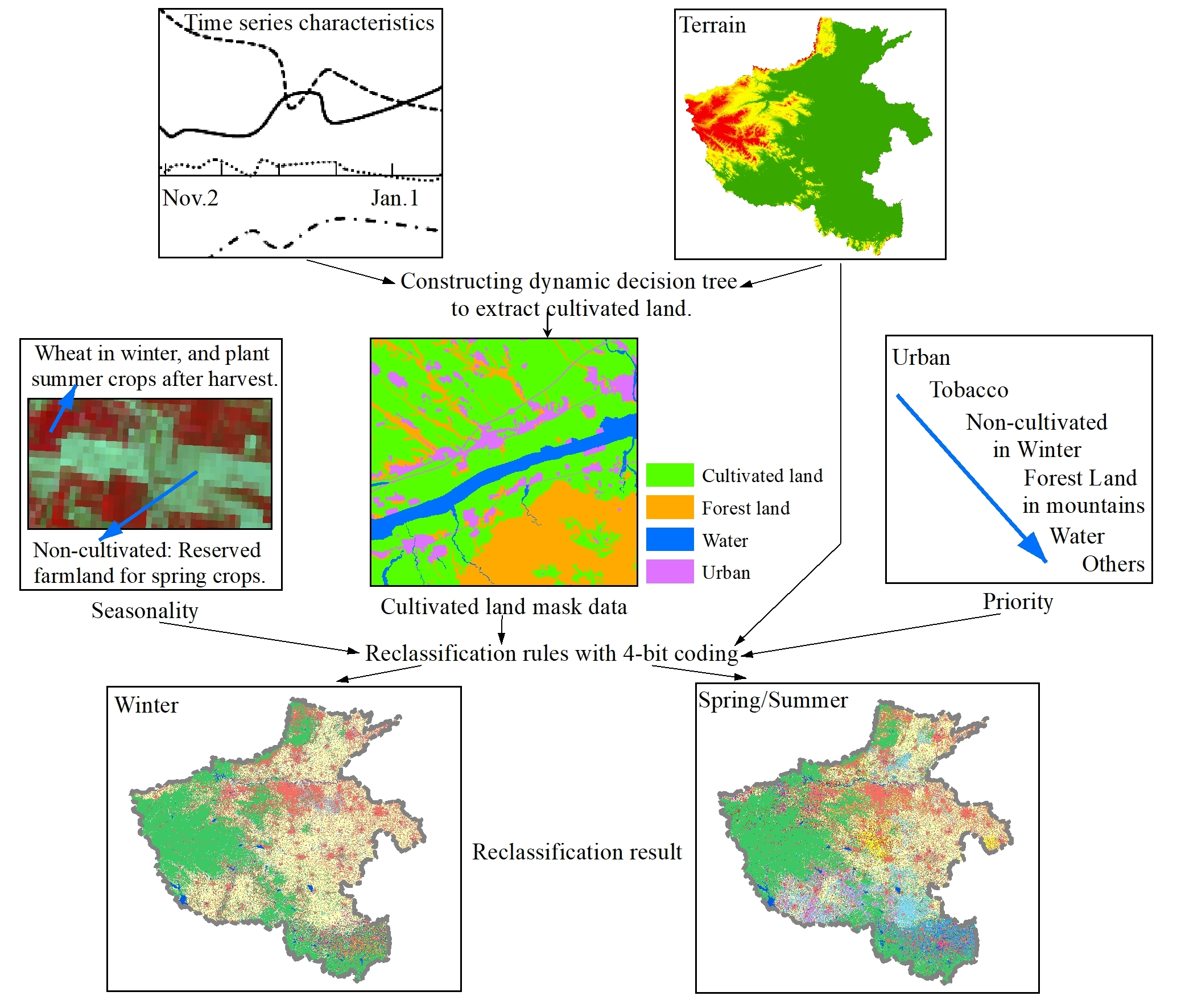
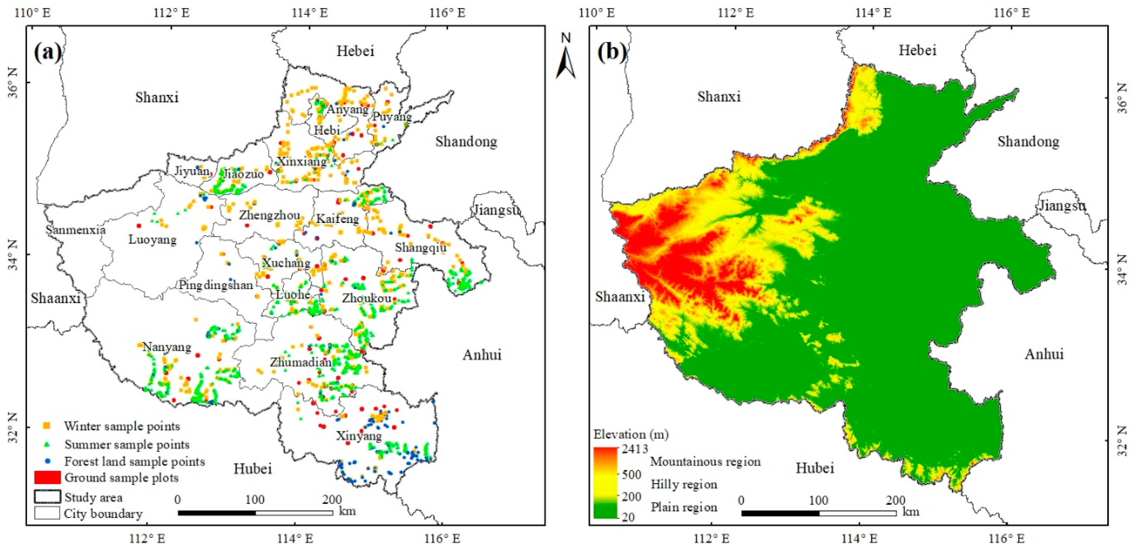
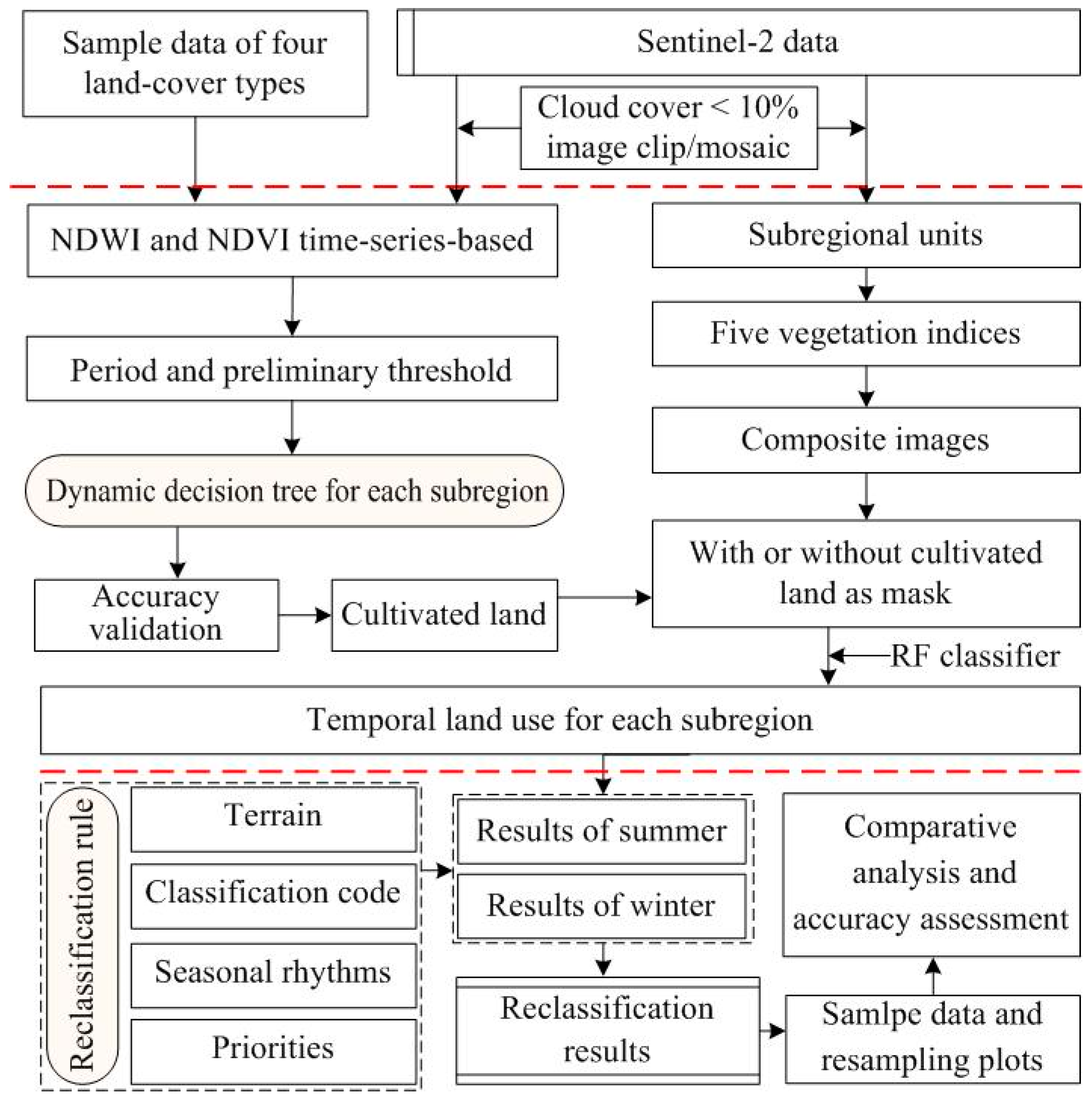
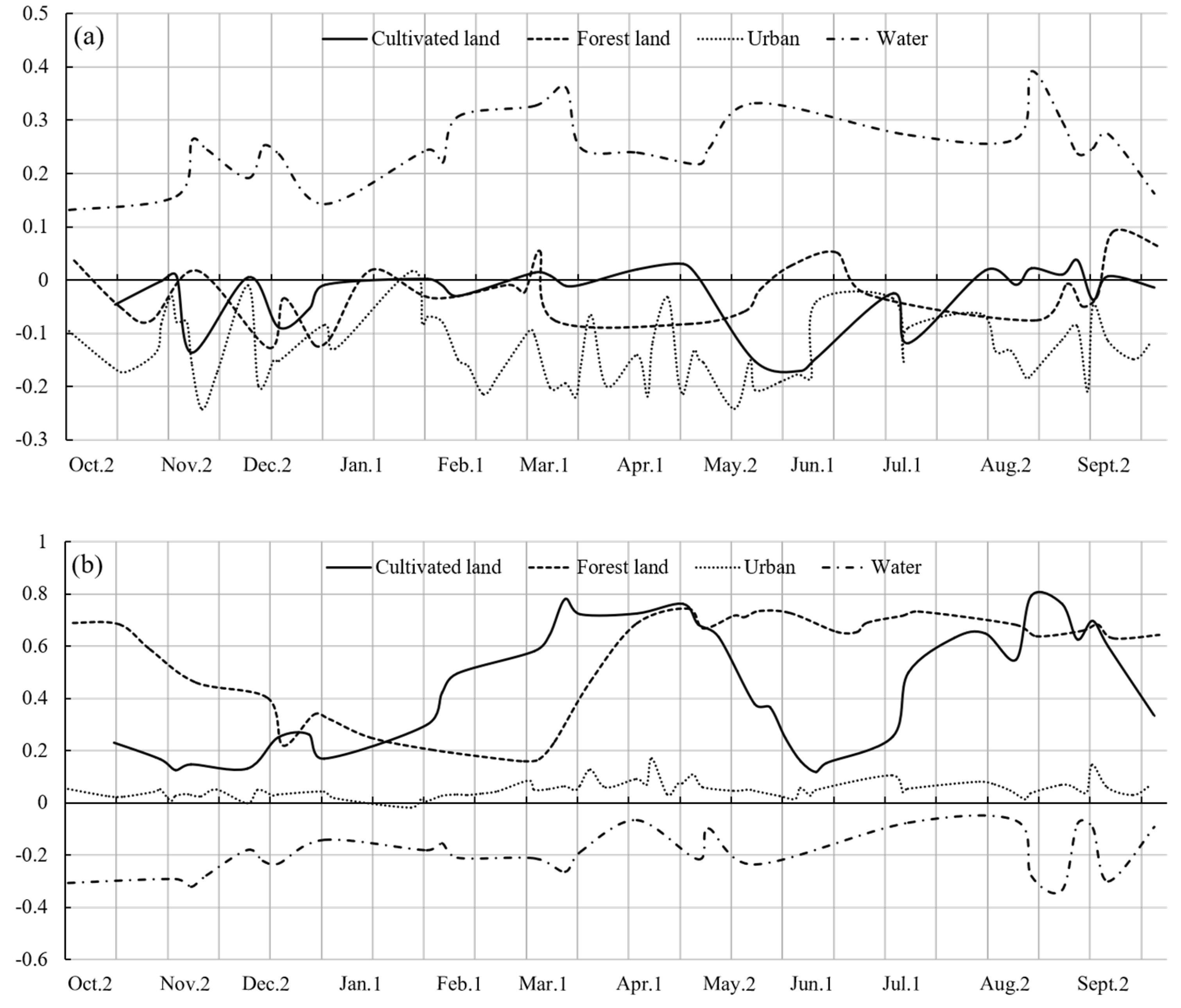
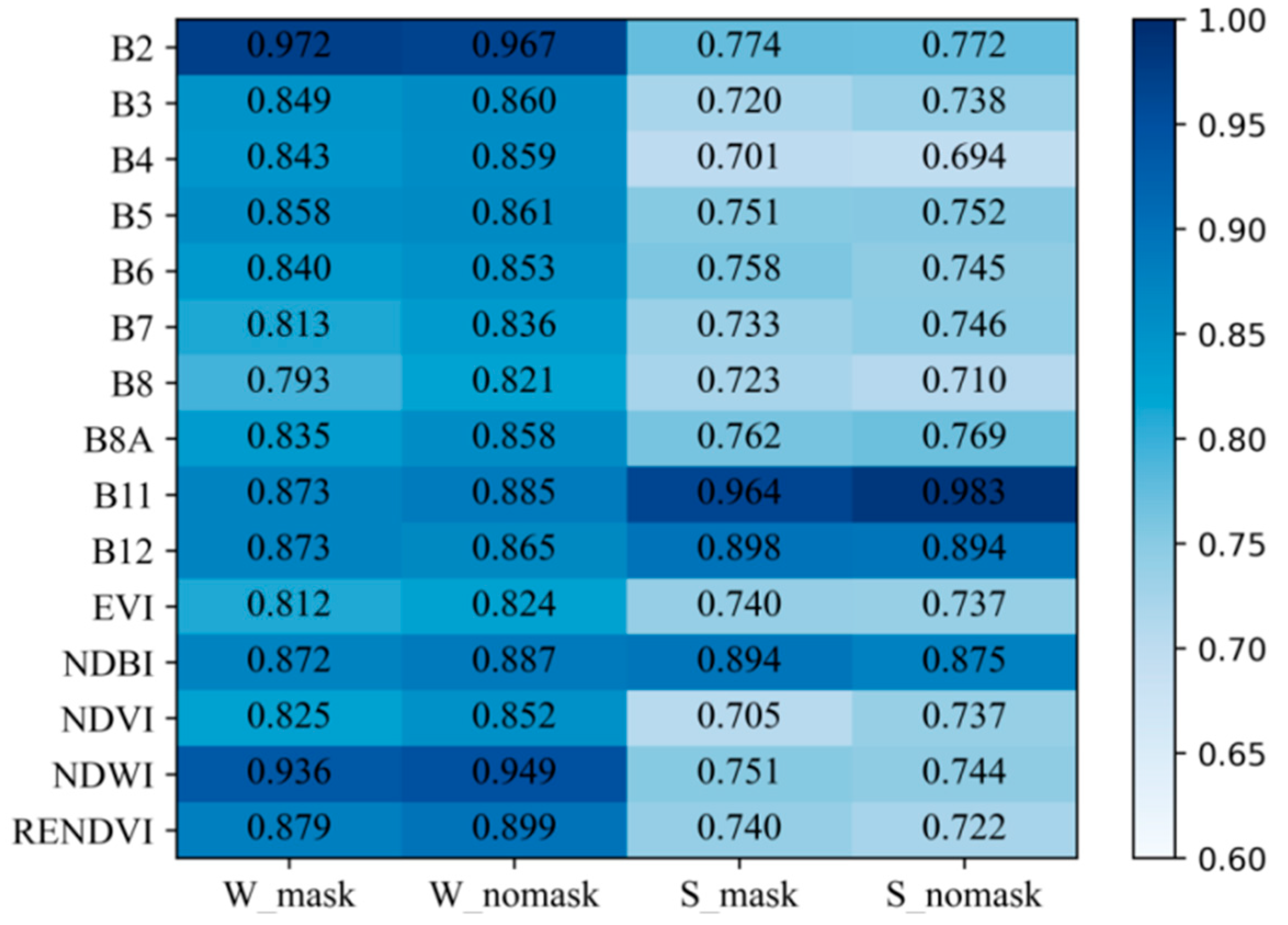
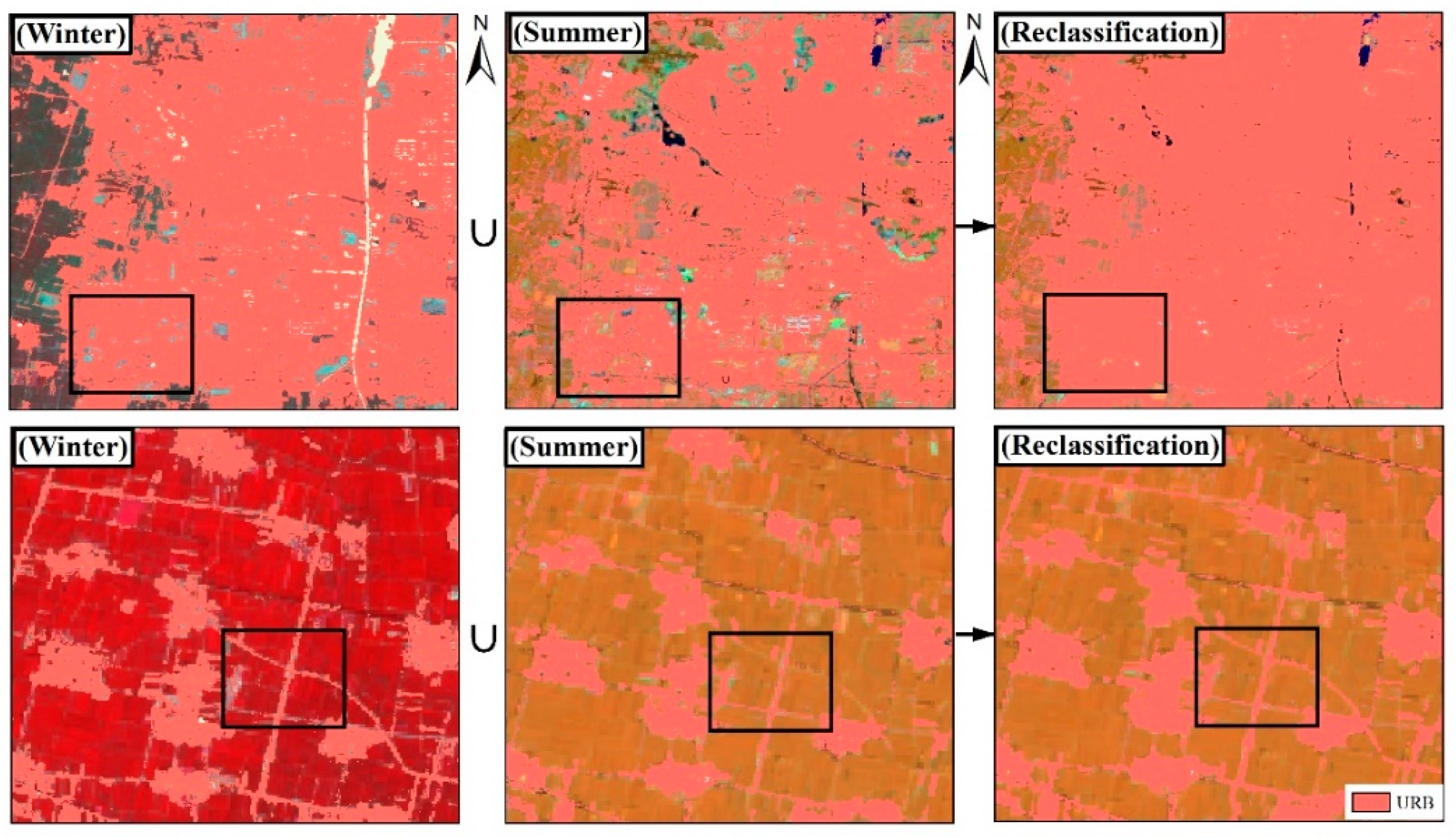
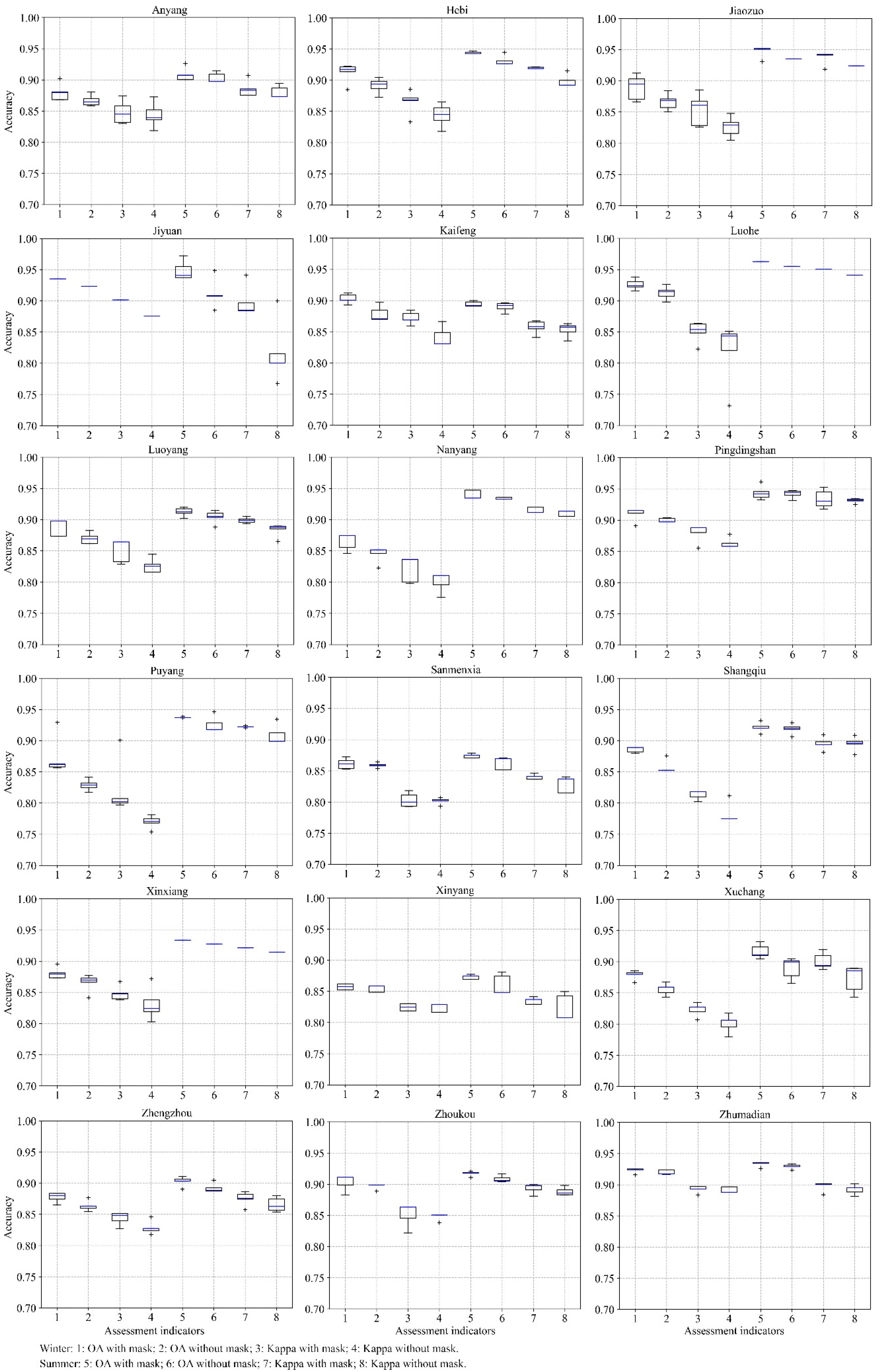
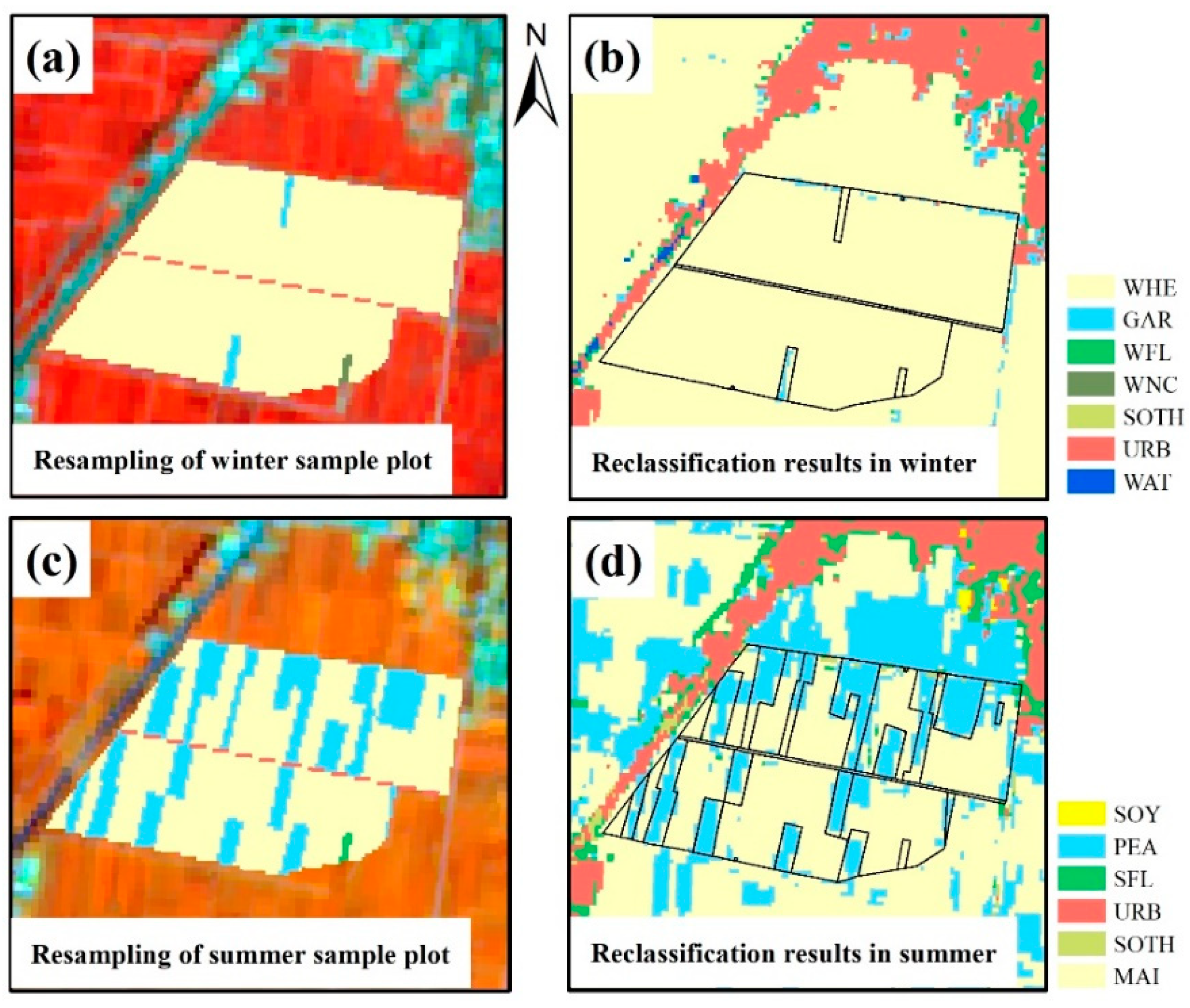
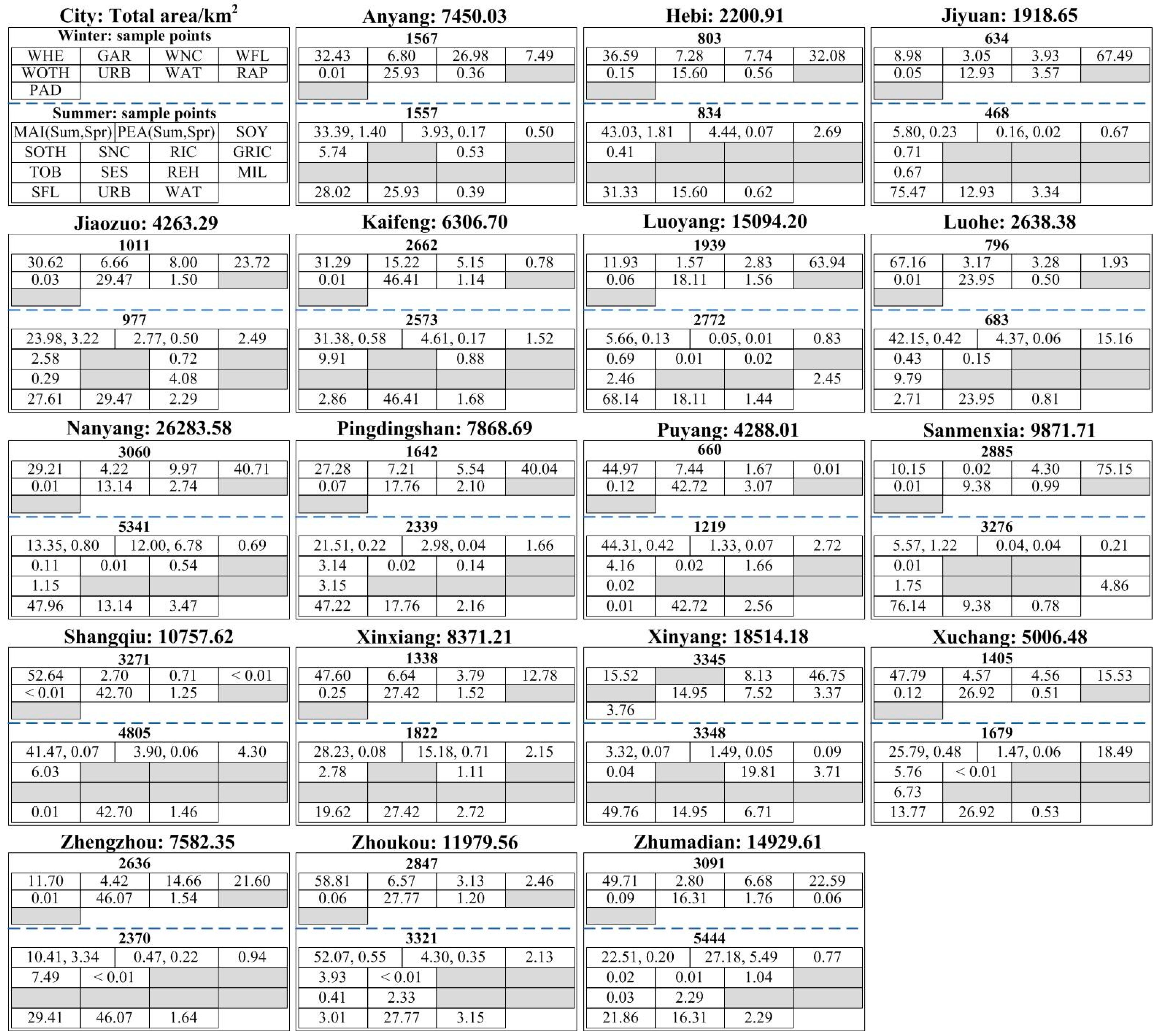
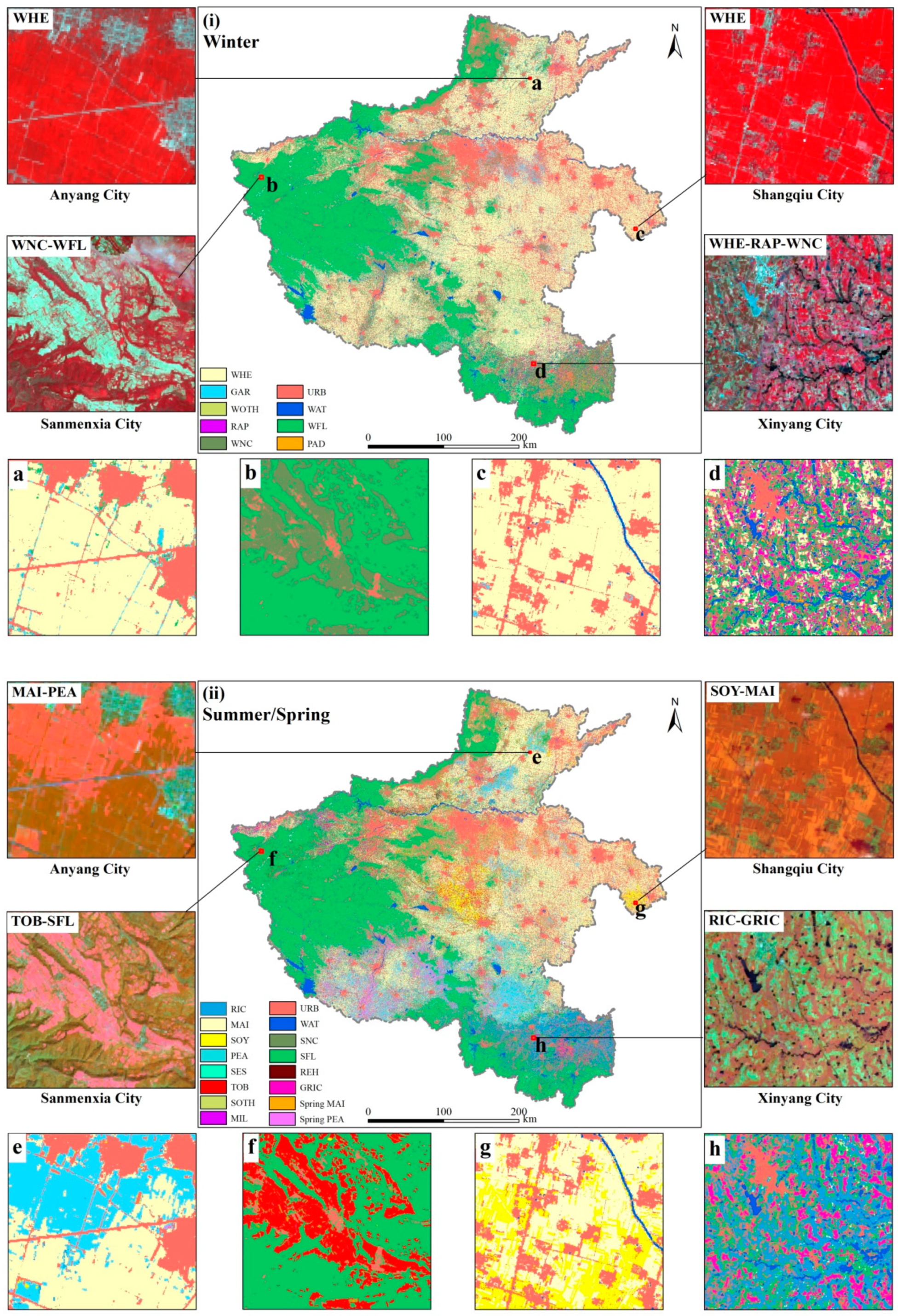
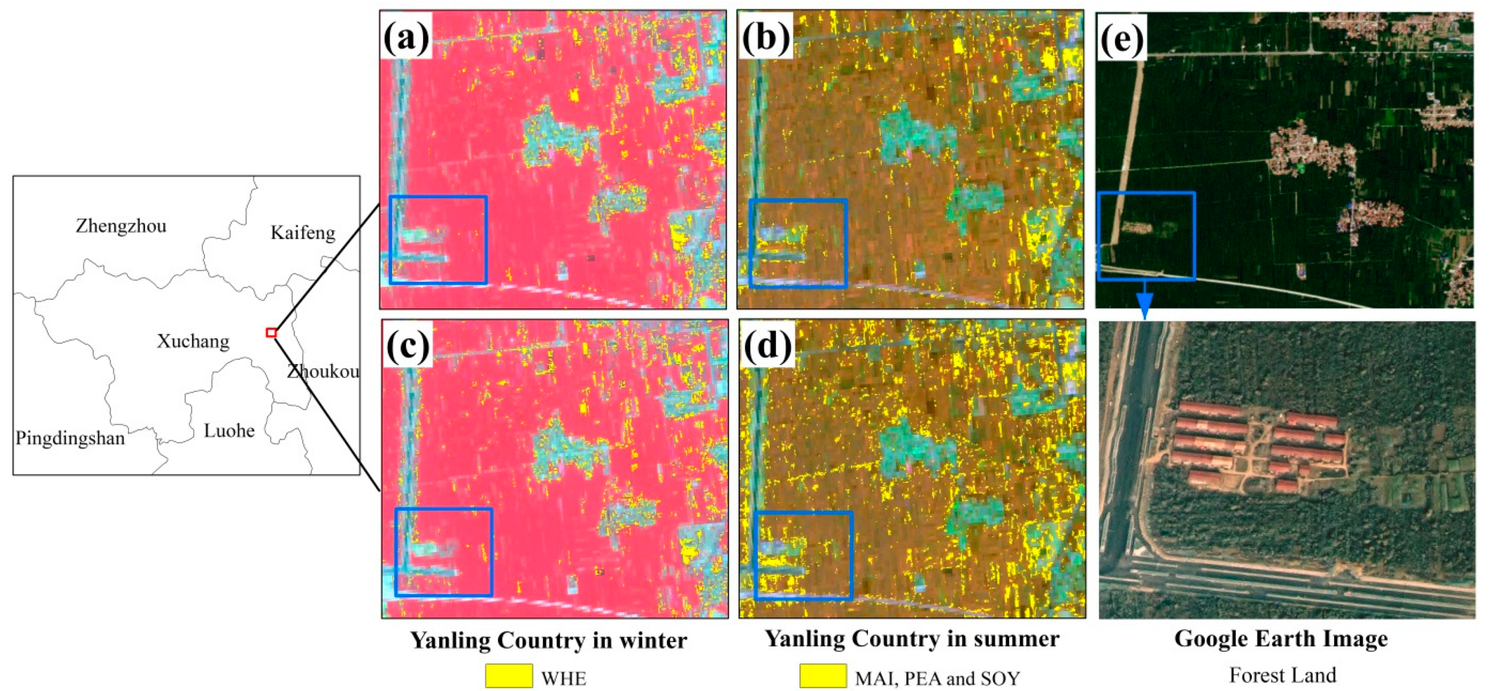
Table 1.
Spectral bands of Sentinel-2 imagery.
| Band | Central Wavelength (nm) | Resolution (m) | Spectral Region |
|---|---|---|---|
| B1 | 443.9(S2A)/442.3(S2B) | 60 | Aerosols |
| B2 | 496.6(S2A)/492.1(S2B) | 10 | Blue |
| B3 | 560(S2A)/559(S2B) | 10 | Green |
| B4 | 664.5(S2A)/665(S2B) | 10 | Red |
| B5 | 703.9(S2A)/703.8(S2B) | 20 | Red edge 1 |
| B6 | 740.2(S2A)/739.1(S2B) | 20 | Red edge 2 |
| B7 | 782.5(S2A)/779.7(S2B) | 20 | Red edge 3 |
| B8 | 835.1(S2A)/833(S2B) | 10 | Near infrared (NIR) |
| B8A | 864.8(S2A)/864(S2B) | 20 | Red edge 4 |
| B9 | 945(S2A)/943.2(S2B) | 60 | Water vapor |
| B10 | 1373.5(S2A)/1376.9(S2B) | 60 | Cirrus |
| B11 | 1613.7(S2A)/1610.4(S2B) | 20 | Shortwave infrared spectral range 1 (SWIR1) |
| B12 | 2202.4(S2A)/2185.7(S2B) | 20 | Shortwave infrared spectral range 2 (SWIR2) |
| QA10 | — | 10 | — |
| QA20 | — | 20 | — |
| QA60 | — | 60 | Cloud mask |
Table 2.
Ground measured data for the sample plots and points in this study.
| Sowing Season | Landcover Types | Abbreviation | Classification Code | Description | Percentage in Sample Plots (%) | Sample Points |
|---|---|---|---|---|---|---|
| Winter | Wheat | WHE | 1 | Wheat pixels during the observation period | 65.33% | 347 |
| Garlic | GAR | 2 | Planting methods for mulching plastic | 6.81% | 28 | |
| Forest Land | WFL | 3 | Tea garden and nursery stock planted on cultivated land, as well as forests | 3.23% | 42 | |
| Non-cultivated | WNC | 4 | Reserved farmland for spring crops | 11.65% | 52 | |
| Others | WOTH | 5 | Winter vegetables, such as carrots, spinach, plastic shed vegetables and others | 0.44% | 32 | |
| Water | WAT | 7 | Water bodies such as ditches and ponds | 2.05% | — | |
| Rape | RAP | 8 | Minor and scattered planting area | 0.64% | 2 | |
| Paddy field | PAD | 9 | Crops are not planted for some reasons after harvesting rice in Xinyang City | — | 5 | |
| Spring/ Summer | Soybean | SOY | 1 | Concentrated planting in Xuchang City and Yongcheng City | 5.15% | 239 |
| Rehmannia | REH | 2 | Chinese herbal medicine, mainly planted in Wenxian County, Jiaozuo City | 0.44% | 9 | |
| Peanut | PEA | 3 | Peanut pixels during the observation period | 14.98% | 670 | |
| Forest Land | SFL | 4 | Tea garden and nursery stock planted on cultivated land, as well as forests | 5.21% | 182 | |
| Non-cultivated | SNC | 5 | Bare or idle land during the observation period | 0.02% | 3 | |
| Water | WAT | 7 | Water bodies such as ditches and ponds | 1.11% | — | |
| Others | SOTH | 8 | Pepper, melon, yam, plastic shed vegetables, and others | 6.12% | 191 | |
| Rice | RIC | 9 | It is mainly planted in southern Henan Province | 9.53% | 67 | |
| Tobacco | TOB | 10 | Small amount of planting in a few areas | 2.03% | 29 | |
| Maize | MAI | 11 | A major crop widely planted in summer | 45.13% | 292 | |
| Sesame | SES | 12 | Concentrated planting in Zhumadian City and Zhoukou City | 0.43% | 57 | |
| Millet | MIL | 13 | Concentrated planting in Sanmenxia City | — | 4 | |
| Glutinous rice | GRIC | 14 | Concentrated planting in Xinyang City, and its harvest time is about 15 days earlier than rice | — | 3 | |
| Urban | URB | 6 | Land for construction, such as houses and roads | 9.85% | — |
Table 3.
Dynamic thresholds of forestland/cultivated land and image acquisition date for crop extraction.
Table 3.
Dynamic thresholds of forestland/cultivated land and image acquisition date for crop extraction.
| City | Area Ratio of Different Terrain Regions (%) | NDVI-Based Threshold between Forest Land and Cultivated Land | Image Acquisition Date for Crop Extraction 2020/mm/dd | |||
|---|---|---|---|---|---|---|
| Plain | Hill | Mountainous | Winter | Summer | ||
| Anyang | 67.26 | 23.74 | 9.00 | 0.49 | 03/28–04/20 | 08/10–09/04 |
| Hebi | 79.58 | 18.08 | 2.34 | 0.49 | 04/07–04/17 | 08/10–09/04 |
| Jiyuan | 21.81 | 49.30 | 28.89 | 0.49 | 04/05–05/12 | 08/10–09/04 |
| Jiaozuo | 81.27 | 10.34 | 8.39 | 0.50 | 03/28–04/17 | 08/17–09/04 |
| Kaifeng | 100.00 | — | — | 0.47 | 03/20–05/12 | 08/17–09/04 |
| Luoyang | 8.14 | 39.24 | 52.62 | 0.49 | 03/18–05/17 | 08/10–09/04 |
| Luohe | 100.00 | — | — | 0.48 | 04/12–05/02 | 09/04 |
| Nanyang | 56.15 | 26.57 | 17.28 | 0.52 | 04/12–05/17 | 08/10–09/04 |
| Pingdingshan | 56.27 | 34.15 | 9.58 | 0.49 | 03/28–05/02 | 08/10–09/04 |
| Puyang | 100.00 | — | — | 0.48 | 04/07–05/02 | 08/17–09/04 |
| Sanmenxia | <0.01 | 13.61 | 86.38 | 0.50 | 02/10–04/28 | 08/26–09/02 |
| Shangqiu | 100.00 | — | — | 0.48 | 03/20–04/24 | 08/17–09/06 |
| Xinxiang | 87.28 | 5.96 | 6.76 | 0.48 | 03/28–04/17 | 08/17–09/04 |
| Xinyang | 86.72 | 11.10 | 2.18 | 0.51 | 03/20–05/02 | 08/10–09/06 |
| Xuchang | 87.40 | 11.41 | 1.19 | 0.48 | 04/07–05/02 | 08/10–09/04 |
| Zhengzhou | 60.54 | 31.13 | 8.33 | 0.48 | 04/22–05/02 | 08/10–09/04 |
| Zhoukou | 100.00 | — | — | 0.48 | 04/12–05/02 | 08/10–09/04 |
| Zhumadian | 92.38 | 7.19 | 0.43 | 0.51 | 04/09–05/12 | 08/10–09/04 |
Table 4.
Pixel numbers and proportion for both the reclassification results and resampling results in winter and summer.
Table 4.
Pixel numbers and proportion for both the reclassification results and resampling results in winter and summer.
| Season | Land Types | Pixel Numbers of Reclassification Results | Pixel Numbers of Resampling Plots | Proportion |
|---|---|---|---|---|
| Winter | WHE | 190,630 | 198,578 | 96.00% |
| GAR | 23,022 | 20,695 | 111.24% | |
| WFL | 14,440 | 9722 | 148.53% | |
| WNC | 27,252 | 35,146 | 77.54% | |
| WOTH | 1342 | 1331 | 100.83% | |
| URB | 38,512 | 29,838 | 129.07% | |
| WAT | 6303 | 6181 | 101.97% | |
| RAP | 1892 | 1905 | 99.32% | |
| Summer | SOY | 12,740 | 15,608 | 81.62% |
| REH | 1560 | 1355 | 115.13% | |
| PEA | 40,443 | 44,875 | 90.12% | |
| SFL | 21,012 | 15,741 | 133.49% | |
| SNC | 1 | 48 | 2.08% | |
| SOTH | 23,195 | 18,637 | 124.46% | |
| RIC | 25,222 | 28,658 | 88.01% | |
| URB | 38,512 | 29,838 | 129.07% | |
| WAT | 4244 | 3335 | 127.26% | |
| TOB | 6854 | 6144 | 111.56% | |
| MAI | 127,928 | 137,860 | 92.80% | |
| SES | 1682 | 1297 | 129.68% |
Table 5.
Multi-season area proportion of different landcover types and comparison with the results in 2018 (%).
Table 5.
Multi-season area proportion of different landcover types and comparison with the results in 2018 (%).
| Landcover Types | WFL | URB | WAT | WHE | WNC | GAR | PAD | RAP | WOTH | |||||
| Winter | 31.36 | 22.95 | 2.30 | 32.22 | 6.14 | 4.18 | 0.42 | 0.38 | 0.05 | |||||
| Landcover Types | SFL | URB | WAT | MAI | PEA | RIC | SOTH | SOY | TOB | MIL | GRIC | SES | REH | SNC |
| Summer | 34.58 | 22.95 | 2.61 | 21.34 | 6.67 | 2.58 | 2.41 | 2.00 | 1.07 | 0.51 | 0.42 | 0.38 | 0.10 | 0.01 |
| Spring | — | — | — | 0.68 | 1.69 | — | — | — | — | — | — | — | — | — |
| Crop Types | WHE | MAI | PEA | RIC and GRIC | SOY | TOB | ||||||||
| Reclassification results | 32.22 | 22.02 | 8.63 | 3.00 | 2.00 | 1.07 | ||||||||
| Results in 2018 | 34.37 | 23.47 | 7.20 | 3.72 | 2.31 | 0.57 | ||||||||
Publisher’s Note: MDPI stays neutral with regard to jurisdictional claims in published maps and institutional affiliations. |
© 2021 by the authors. Licensee MDPI, Basel, Switzerland. This article is an open access article distributed under the terms and conditions of the Creative Commons Attribution (CC BY) license (https://creativecommons.org/licenses/by/4.0/).
Share and Cite
MDPI and ACS Style
Wang, L.; Wang, J.; Qin, F. Feature Fusion Approach for Temporal Land Use Mapping in Complex Agricultural Areas. Remote Sens. 2021, 13, 2517. https://0-doi-org.brum.beds.ac.uk/10.3390/rs13132517
AMA Style
Wang L, Wang J, Qin F. Feature Fusion Approach for Temporal Land Use Mapping in Complex Agricultural Areas. Remote Sensing. 2021; 13(13):2517. https://0-doi-org.brum.beds.ac.uk/10.3390/rs13132517
Chicago/Turabian StyleWang, Lijun, Jiayao Wang, and Fen Qin. 2021. "Feature Fusion Approach for Temporal Land Use Mapping in Complex Agricultural Areas" Remote Sensing 13, no. 13: 2517. https://0-doi-org.brum.beds.ac.uk/10.3390/rs13132517
Note that from the first issue of 2016, this journal uses article numbers instead of page numbers. See further details here.