
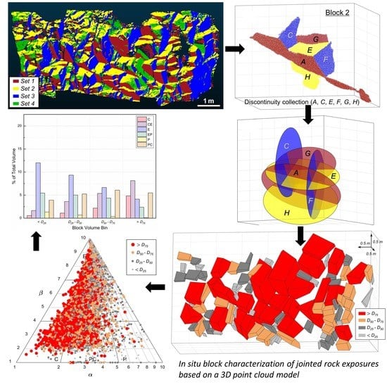
In-Situ Block Characterization of Jointed Rock Exposures Based on a 3D Point Cloud Model


1
Department of Geotechnical Engineering, College of Civil Engineering, Tongji University, Shanghai 200092, China
2
Key Laboratory of Rock Mechanics and Geohazards of Zhejiang Province, Shaoxing University, Shaoxing 312000, China
3
Department of Geotechnical Engineering, National Technical University of Athens, 15780 Athens, Greece
4
School of Earth and Environment, University of Leeds, Leeds LS2 9JT, UK
*
Author to whom correspondence should be addressed.
Remote Sens. 2021, 13(13), 2540; https://0-doi-org.brum.beds.ac.uk/10.3390/rs13132540
Submission received: 10 May 2021
/
Revised: 18 June 2021
/
Accepted: 26 June 2021
/
Published: 29 June 2021
(This article belongs to the Special Issue UAV-Based Photogrammetry and Measurements for Monitoring Natural Hazards and as a Risk Reduction Measure)
Abstract
:The importance of in-situ rock block characterization has been realized for decades in rock mechanics and engineering, yet how to reliably measure and characterize the geometrical properties of blocks in varied forms of exposures and patterns of jointing is still a challenging task. Using a point cloud model (PCM) of rock exposures generated from remote sensing techniques, we developed a consistent and comprehensive method for rock block characterization that is composed of two different procedures and a block indicator system. A semi-automatic procedure towards the robust extraction of in-situ rock blocks created by the deterministic discontinuity network on rock exposures (PCM-DDN) was developed. A 3D stochastic discrete fracture network (DFN) simulation (PCM-SDS) procedure was built based on the statistically valid representation of the discontinuity network geometry. A multi-dimensional block indicator system, i.e., the block size, shape, orientation, and spatial distribution pattern for systematic and objective block characterization, was then established. The developed method was applied to a synthetic model of cardboard boxes and three different rock engineering scenarios, including a road cut slope from Spain and two open-pit mining slopes from China. Compared with existing empirical methods, the proposed procedures and the block indicator system are dependable and practically feasible, which can help enhance our understanding of block geometry characteristics in related applications.
1. Introduction
The presence and mutual intersection relationship of discontinuities form in-situ rock blocks with various 3D geometries in a jointed rock mass [1,2]. The size, shape, and spatial distribution of rock blocks have a significant impact on the engineering properties of rock masses [2,3,4,5,6], the failure scale and mode in most natural rock collapse hazards [7,8], and rock engineering activities, such as high-steep slope construction [9,10] and underground excavation [11,12]. The International Society for Rock Mechanics and Rock Engineering (ISRM) listed the block size as a critical parameter controlling the rock mass behavior [13]. Although the importance of in-situ block characterization has been realized for decades and various methodologies and indicators have been continually developed by many researchers [14,15,16,17,18], there still lacks widely recognized procedures or universal standards [5]. How to best measure and characterize in-situ block properties, e.g., in-situ block size distribution (IBSD) in varied forms of exposures and patterns of jointing, is still a tough challenge in rock mechanics and engineering [3,19,20].
Palmstrom [3] presented a practical overview of various measurements of the intensity of jointing, which considered rock quality designation (RQD) [21], volumetric joint count () [22,23], or weighted joint density (wJd) [24] as different perspectives of block size assessment. These spacing-derived indices have been extensively applied to describe rock mass integrity, particularly in rock mass quality classification systems, yet providing no specific block size value. Şen and Eissa [25] ideally categorized block shapes into three different types, namely, bars, plates, and prisms, and established analytical charts of , RQD, and average block volume for each type. A renowned block volume estimation () for rock masses containing three discontinuity sets was later introduced by Cai et al. [26] as follows:
where , , and are the normal set spacings of the three discontinuity sets; , , and are the intersection angles between three sets; and , , and are the persistence factors of three sets.
Benefiting from Monte Carlo discrete fracture network (DFN) modeling, a general methodology for IBSD assessment has been adopted by many scholars [5,14,27]. Instead of acquiring only a single value (i.e., the average block volume), the cumulative distribution curve of block sizes can be produced from DFN simulations.
The natural variability and spatial distribution of individual blocks on a rock face have a defining influence on rock failures. For example, the volume and velocity of detachable blocks determine the intensity of fragmental rockfalls [28]. Consequently, great efforts have been devoted to utilizing deterministic field discontinuity data directly for IBSD estimation. Wang et al. [29] and Lu and Latham [19] introduced two methods (i.e., the dissection method and the equation method) for IBSD assessment from scanline surveys. The dissection method extracts blocks that originate from scanline-obtained intersecting discontinuity planes within a predefined bounding box. All studied discontinuities are defined as infinitely persistent, and the blocks are simultaneously cut by virtual box boundaries. The equation method is only suitable for rock masses possessing three discontinuity sets, and possible variations in the type of spacing distribution and dispersion of orientation within three sets are not taken into account. Saroglou et al. [30] labeled the main discontinuity planes on slopes and delineated the potentially unstable rock blocks for rockfall risk appraisal. Jern [31], Stavropoulou [32] and Stavropoulou and Xiroudakis [33] derived closed-form IBSD expressions within a rock mass transected by three sets based on different hypotheses.
The above review outlines the progresses in techniques for block size assessment. However, one or more limitations exist among these studies that restrict their broader applications. For example, most equation methods or analytical formulae focus on the mean block size calculation. Using only a certain value is apparently insufficient to describe the structural complexity of an entire rock mass and these methods can only be implemented with limited discontinuity sets (e.g., three sets). Furthermore, most methods require oversimplified treatments and approximations without considering the statistical nature of discontinuity geometry (e.g., defined as being infinitely persistent), and no relevant indication of block shape characteristics is provided [2].
Regardless of which method is chosen, a thorough understanding of the fundamental discontinuity parameters is always required. Hence, organizing unbiased and objective field investigation is the foundation to deduce the real-life status of rock blocks. The conventional survey may suffer various impediments related to access restrictions, data deficiencies, manual measurement bias, safety risks, and labor-intensive operating environments. Especially for geologically hazard sites or ongoing open-pit mines, a large number of measurements for structural characterization are almost impossible due to these restrictions and risks [28].
With the rapid advances in remote sensing techniques, e.g., light detection and ranging (LiDAR, including airborne and terrestrial laser scanning) and digital photogrammetry, which can generate high-resolution 3D products (e.g., point cloud model, PCM), several manual or (semi-) automatic methods for the identification and characterization of discontinuities have been developed to overcome the above limitations [34,35,36,37,38]. These techniques also offer improved practical means to investigate rock blocks from 3D digital outcrop models [5,8,16,20]. For example, Abellán et al. [39] presented the volume calculation for several specific blocks based on a terrestrial laser scanning model. Vanhaekendover et al. [40] proposed a voxel approach to estimate IBSD using persistent discontinuities on the rock face. Mavrouli et al. [41] extracted discontinuity information manually based on a digital elevation model with a terrestrial laser scanner and then estimated the IBSD by calculating the equivalent volume of the prisms. Chen et al. [16] established a block extraction method from PCM by assuming block shapes as hexahedron. These methods simplify blocks to regular shapes for IBSD estimation; hence, the accuracy of the results is far from guaranteed. A recent review article by Battulwar et al. [42] also pointed out that “there is a lack of efficient algorithms for direct computation of block size from 3D rock mass surface models”.
To address the above-mentioned problems, here, we present a state-of-the-art method integrating close-range remote sensing technology with several novel computing algorithms for rock block characterization. First, a remote measurement technique based on the PCM of rock exposures is established, delivering the exact location, orientation, persistence and spacing of discontinuities at arbitrary positions. The representative values of fundamental parameters and their best-fitted statistical functions are acquired. Then, two block characterization procedures based on PCM and digital discontinuity mapping from measured and simulated perspectives are introduced: (1) a semi-automatic procedure towards the robust extraction of in-situ rock blocks created by the deterministic discontinuity network on rock exposures (PCM-DDN) is developed. These are the individual blocks that under given conditions may detach and trigger surface failure phenomena. (2) Based on the statistically valid representation of the discontinuity network geometry, a 3D stochastic DFN simulation (PCM-SDS) procedure is developed for block characterization. A multi-dimensional block indicator system for comprehensive block characterization, i.e., IBSD, block shape distribution (BSD), and block orientation distribution (BOD), is introduced, and the exposed block spatial distribution (EBSD) is mapped. A consistency assessment of IBSD, BSD, and BOD obtained from the two procedures is implemented. The developed procedures are applied to a synthetic model of cardboard boxes and three different rock engineering scenarios, including a road cut slope from Spain and two open-pit mining slopes from China. The applicability, advantages, and disadvantages of the two procedures are discussed. A comparison with the analytical approach developed by Cai et al. [26] is also presented.
2. Study Sites
2.1. Site 1: A Road Cut Slope in Catalonia, Spain
The studied road cut slope is located in the south of Torroja del Priorat along road no. TP7403, which is near the northern limit of the Baix Camp region of Catalonia, Spain [43]. This site is mainly composed of sandstones of Carboniferous age. The size of the entire study area is approximately 9.2 by 5.1 m.
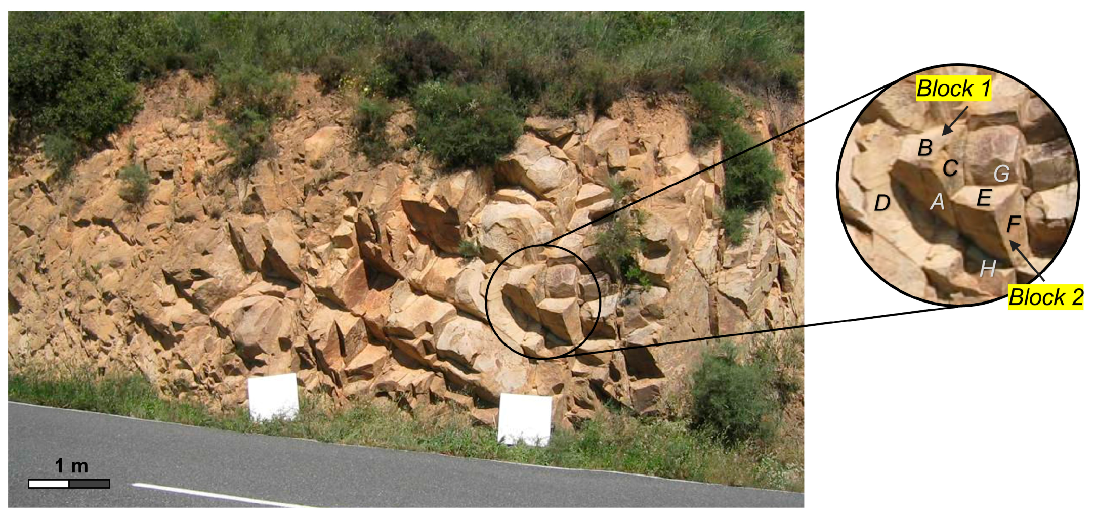
The Optech ILRIS-3D laser scanner was utilized for 3D point cloud data collection, and a total of 1.6 million points were acquired with a resolution of approximately 6 by 6 mm. The point cloud data were stored in the XYZ format, with four columns containing the x, y, and z coordinates and the intensity values, respectively. As shown in Figure 1, the study area of the slope is covered by sparse vegetation, and the discontinuities are well developed, which make exposures of these rocks well suited to demonstrate the methodologies presented in Section 3.
2.2. Site 2: Yinshan Open-pit Copper Mine in Dexing, China
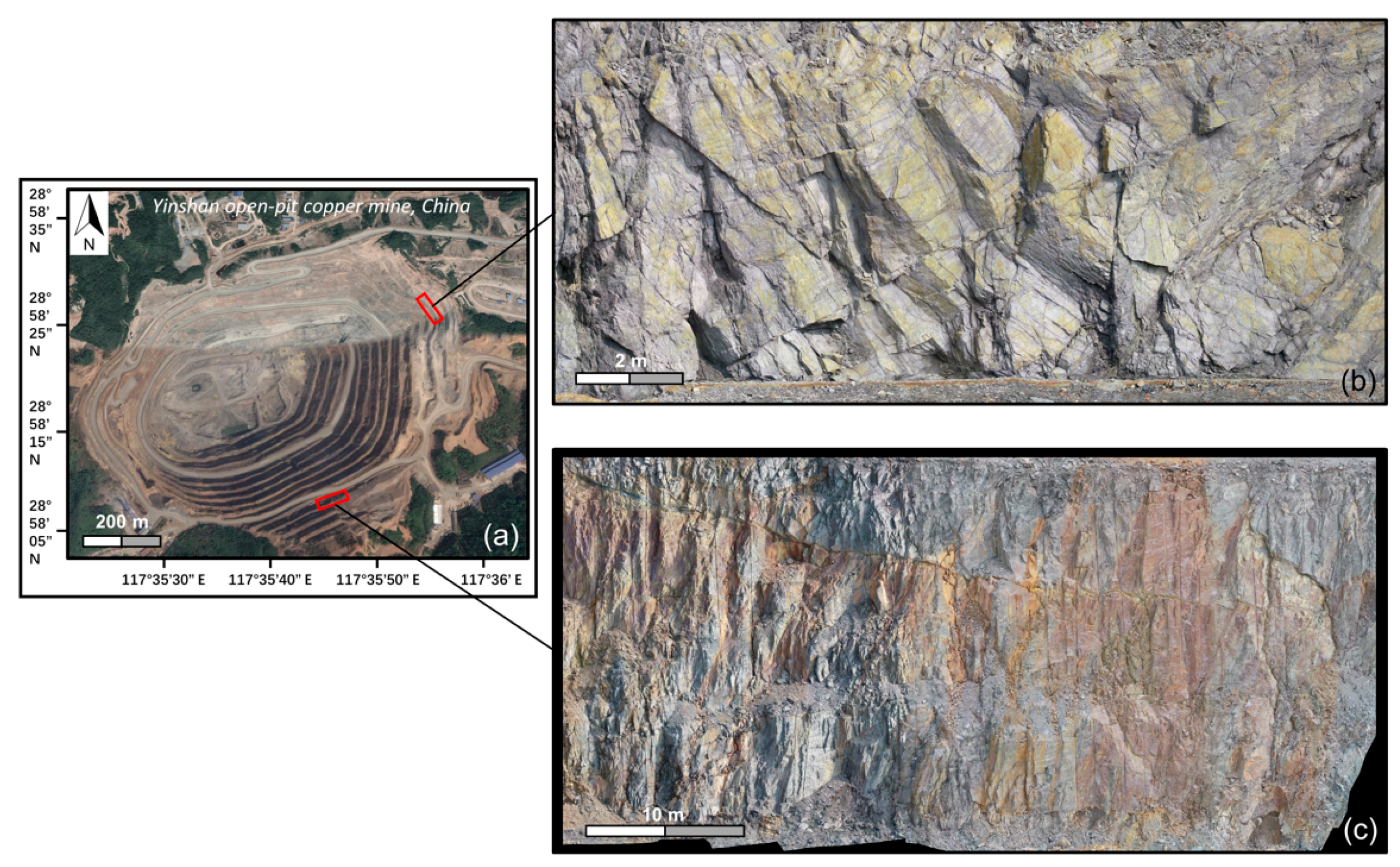
The Yinshan open-pit copper mine is located in Dexing city, northeast of Jiangxi Province, China (Figure 2a). Two slopes with different surface conditions were selected. The eastern slope (Figure 2b) is sub-vertical (inclination: 80°–90°) and is mainly composed of sericite phyllite and quartz porphyry. This slope is fractured by several joint sets and is vulnerable to rockfall and avalanche disasters. According to past monitoring records, rockfalls occurred frequently along discontinuities, and the major failure mechanism was associated with wedge [44]. The southern slope (Figure 2c) is also sub-vertical (inclination: 80°–85°) and is mainly composed of sericite phyllite. Due to the adopted smooth blasting technique, it was rare to find unbroken blocks at the slope face.
A UAV (unmanned aerial vehicle) digital photogrammetry survey was applied at this site using a DJI Phantom 4 Pro UAV equipped with an on-board camera. A total of 272 and 253 digital images from a horizontal camera view were acquired for the eastern and southern slopes, respectively. The structure-from-motion (SfM) technique was employed for high-resolution PCM generation. A detailed description of this technique can be found in Westoby et al. [45], Giordan et al. [46], and Kong et al. [47]. Dense point cloud datasets of two slopes were produced and georeferenced in a geodetic coordinate system. The resolutions were approximately 5 by 5 mm for both slopes.
2.3. A Synthetic Test Model: The Dataset of Cardboard Boxes
Several cardboard boxes with different sizes were assembled and taped in the laboratory, as shown in Figure 3a. The boxes were scanned by a TOPCON Laser Scanner GLS-2000. After the pre-processing operations (e.g., point cloud registration and denoising), a total of 556,815 points were acquired with a resolution of approximately 2 by 2 mm (Figure 3b).
Since the sizes of all experimental boxes were precisely known, this synthetic box model was used to make the comparison between the proposed extraction algorithms and the true geometries of the boxes, then to evaluate the effectiveness of this method. The comparison results are presented in Section 4.
3. Methodology
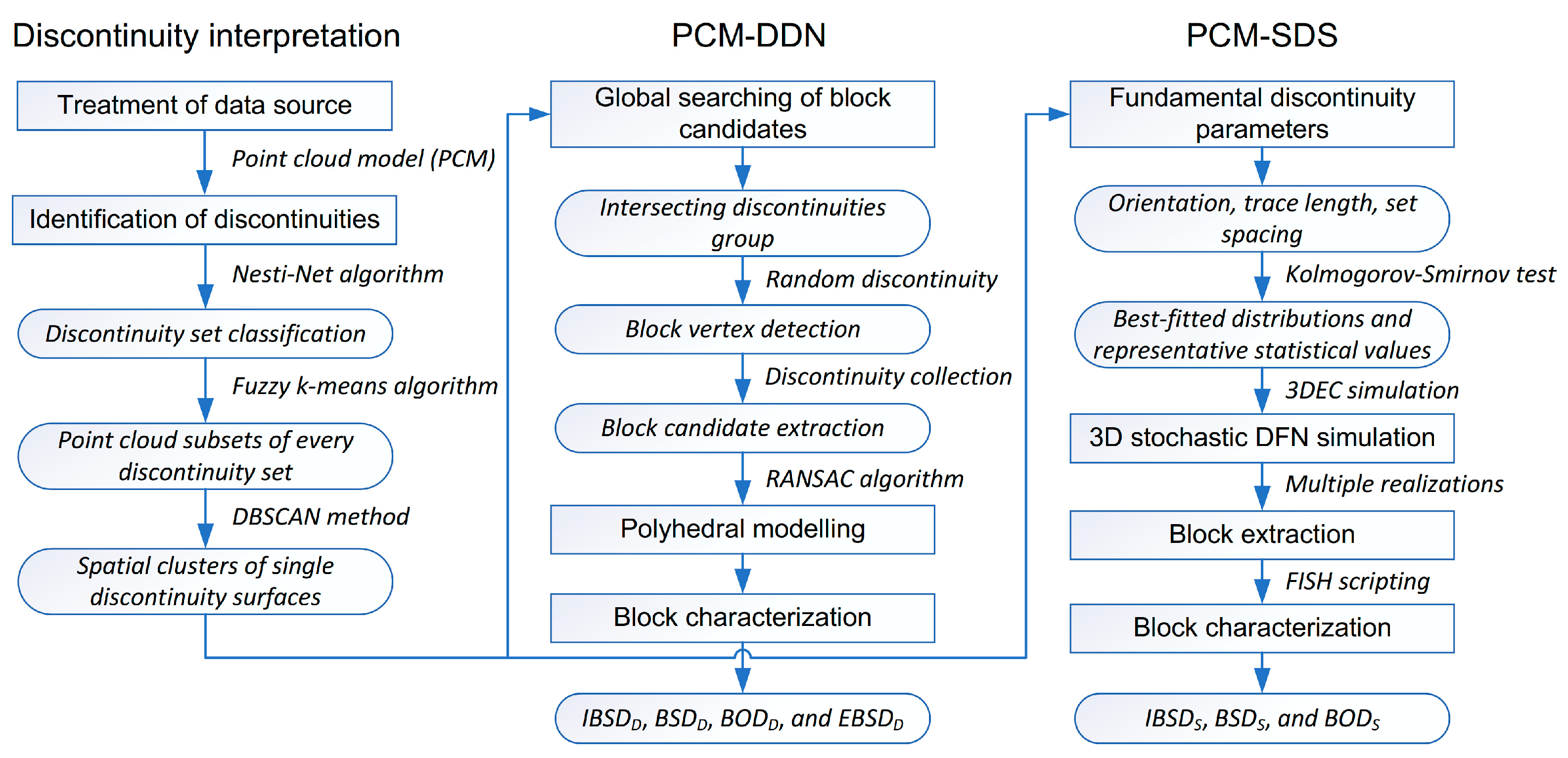
The flow chart of methodology is illustrated in Figure 4. Several mathematical algorithms were designed and programmed for discontinuity interpretation and block characterization.
3.1. Treatment of Data Source
With regard to digitally identifying discontinuities, many scholars have explored diverse approaches, mainly containing two processing treatments of PCM: (1) surface reconstruction, such as triangulated irregular network (TIN) meshing technology [48,49,50], and (2) raw point cloud utilization [8,16,34,51]. On account of the impact of environmental factors (e.g., limited sensor range, inevitable occlusions, and moving objects or scanning angle), any PCM of rock exposures measured with LiDAR or digital photogrammetry is non-uniformly sampled, and it is likely that the final scanned model will contain undersampled areas. The varying sampling density of the PCM will eventually influence the accuracy of the TIN meshing surface. More importantly, rock surfaces always preserve many large-scale undulations and small-scale roughness, and the meshing operation will induce irregularities at these uneven (or sharp) features [16,52]. Therefore, instead of producing a derivative meshed model, the raw point cloud dataset was directly applied here.
3.2. Identification of Discontinuities from PCM
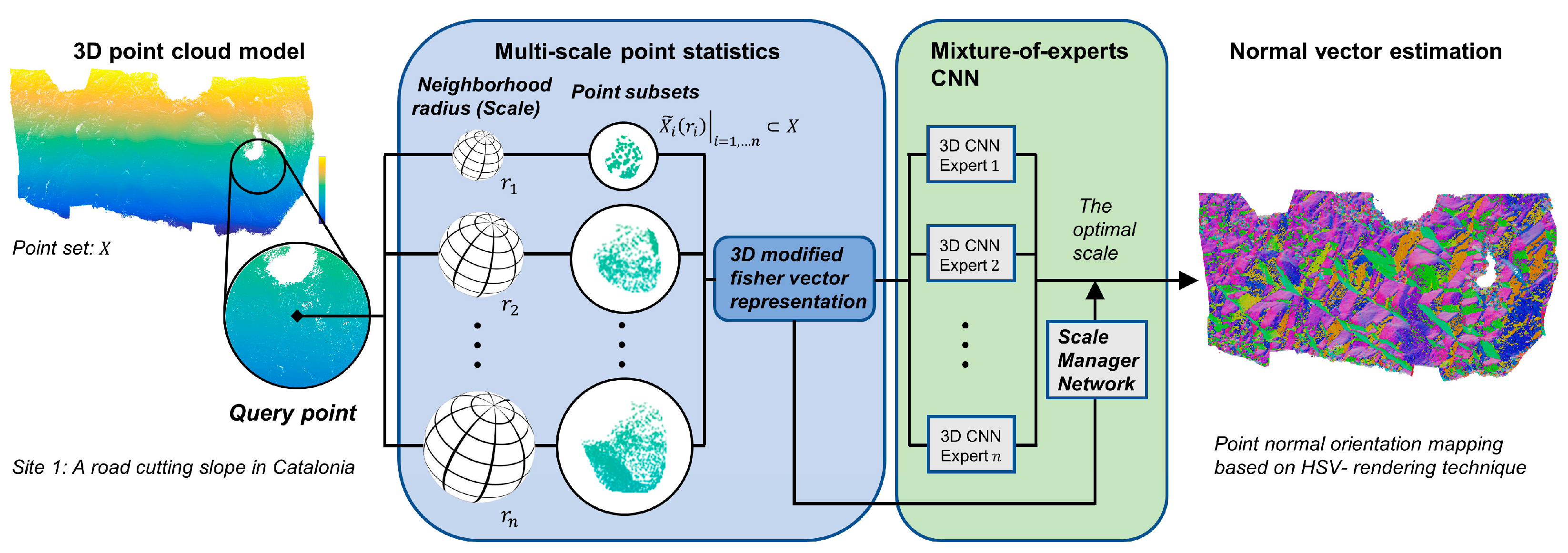
Assembling the corresponding points that belong to discontinuity surfaces correctly from the PCM is a key step for modeling the in-situ structural network of rock masses. First, the directions of every point were estimated by calculating their normal vectors in 3D space. A state-of-the-art normal estimation for unorganized PCM using convolutional neural networks (CNNs), called Nesti-Net [53], was utilized. The scheme of the Nesti-Net algorithm is outlined in Figure 5. Different point subsets that refer to scales with different neighborhood radii were extracted from the point cloud dataset. These scales were independently translated and uniformly fitted into a zero-centered unit sphere, and then the 3D modified Fisher vector representation was calculated for each scale relative to a Gaussian grid structure [54]. The local multi-scale representation of pointwise statistics served as an input to a 3D mixture-of-experts CNN architecture, and the normal vector of each point was estimated as output.
To demonstrate the main direction of the rock surface clearly, normal vector orientation mapping was illustrated based on the HSV (for hue, saturation, value) rendering technique [55]. The Nesti-Net algorithm significantly increases the robustness and accuracy of normal estimation under different noise conditions, particularly when dealing with rock exposures that possess undulations and roughness.
Subsequently, the transformation between the normal vector in Cartesian coordinates and the related orientation of each point (dip direction and dip angle ) was established, which is given by
where , and are three direction cosines of a unit vector. is determined as: , if , and ; , if , and ; , if and or if , and .
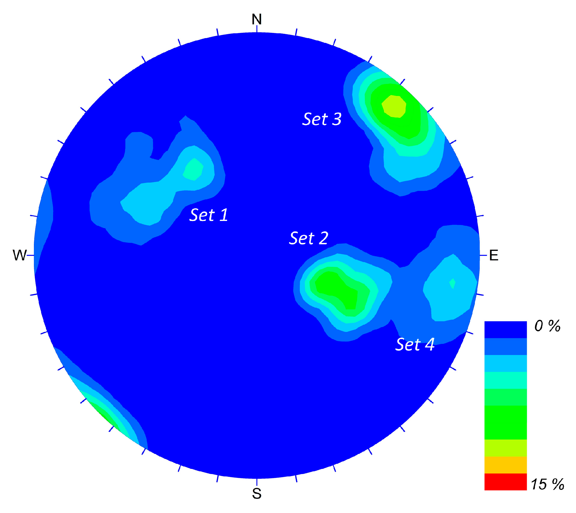
All orientations were clustered in stereographic projection by the fuzzy k-means algorithm [56] to identify the main discontinuity sets and group-associated points of each set. The fuzzy k-means algorithm is a partitional clustering technique that has been successfully applied to orientation grouping by several researchers [43,49,57]. It yields the automatic assignment of similarly oriented data into one group. In the fuzzy k-means structure, each independent variable is appointed a degree of membership (from 0 to 1) to each cluster core, the algorithm determines membership by angular similarity between measurements with a predefined number of clusters, and no other measurable or empirical variables are required. Subsequently, the outliner data (i.e., non-discontinuity surface data) can be discarded using the maximum angle filter method [34,43]. As shown in Figure 6a, four discontinuity sets were classified at Site 1, and the points associated with their family set are represented in the same color.
Each spatial cluster of a single discontinuity surface can be extracted from the point subset of an affiliated set manually or automatically, such as using the well-known density-based spatial clustering of applications with noise (DBSCAN) method [58,59] or the density-ratio-based algorithm [51,60]. The DBSCAN method has been successfully verified for the processing of LiDAR point clouds in rock engineering applications [34,61]. Here, the DBSCAN method was operated first, and visual inspection and modification based on the actual situation were conducted manually afterwards to reduce extraction errors. The user’s supervision guaranteed that the neighboring points that form the same discontinuity surface are indeed merged together properly. Finally, every deterministic discontinuity surface from each set was acquired in this step. The individual discontinuities were assigned as members of their family set. For example, each individual discontinuity of Set 1 was separated and delineated using different colors (Figure 6b).
3.3. PCM-DDN: Global Searching of Block Candidates
To identify the rock blocks on a rock exposure, at least three dimensions of a rock block dissected by the discontinuity network should be revealed. The assembly of intersected discontinuity surfaces that form faces of one block were searched in this step. The main process was performed as follows: (1) intersecting discontinuities group, (2) block vertex detection, and (3) block candidate extraction.
In reality, if two discontinuity surfaces intersect, some points from two discontinuity point clusters will be adjacent in the PCM. A parameter Interdist was introduced to specify the maximum distance value between two intersecting point clusters. If the distance of two points from two discontinuity point clusters is less than Interdist, these two discontinuity point clusters are considered to intersect. Normally, the value of Interdist is chosen to be slightly larger than the original resolution (i.e., the point interval). For example, the parameter Interdist of Site 1 was set to 10 mm, and after a global cyclic search, discontinuity B (Figure 1) was detected to intersect with discontinuities A, C, and D in Figure 7a, and discontinuity E (Figure 1) intersected with discontinuities A, C, G, and F in Figure 7d. Hence, the lists of every individual discontinuity with its intersecting discontinuities can be acquired.
The block vertex can be identified by searching at least three intersecting discontinuities that share common discontinuities with each other. For example, the intersecting discontinuity list that involves discontinuity A can be expressed as (A, B; A, C; A, D; A, E; etc.). If discontinuities B and C intersect with each other, then discontinuities A, B, and C are registered as block vertices (A, B, C). This process was repeated until all block vertices exposed on the rock face were detected.
If the block vertices belong to the same block, they are subsequently merged together. For example, two block vertices (A, C, E) and (A, E, F) were merged to a larger discontinuity collection (A, C, E, F) of Block 2 (Figure 7d). Traversing through the list of all block vertices, all block candidates and their affiliated discontinuity collections from the rock face were extracted. The discontinuity collections of Blocks 1 and 2 (Figure 1) are demonstrated in Figure 7a,d. In some cases, the rock blocks may be partly cut by random discontinuities, and these discontinuities can also be added to the corresponding collections.
3.4. PCM-DDN: Polyhedral Modeling
The random sample consensus (RANSAC) algorithm [62] was employed for executing plane fitting of individual discontinuities. RANSAC is an iterative mathematical algorithm that is capable of fitting a set of 2D or 3D spatial data containing outliers (or noise) into a specific geometric model such as a line, a plane or a sphere. Due to its capability to tolerate a tremendous fraction of outliers, RANSAC can take the roughness and waviness of discontinuity surfaces into account and offer a more reasonable computation. One example of discontinuity A and its fitting plane equation are shown in Figure 6c.
One primary issue for the PCM-DDN method is that there are always some parts of rock blocks invisible on the rock face; for most of them, one can make a logical extension of existing discontinuity planes into the rock mass to form the 3D block geometry, as shown in Figure 7b,e; for some special cases, artificial planes are needed to create blocks based on the on-site practical situation and the geological expertise of geologists.
With the best-fitting planes of one complete discontinuity collection of a block, polyhedral modeling including all vertices, edges and faces can be established from mutual intersections of discontinuity planes. As an example, the polyhedral models of Blocks 1 and 2 are shown in Figure 7c,f.
3.5. PCM-DDN: Block Characterization
The intersection of discontinuity planes produces rock blocks with various shapes, most of which, in general, have more than four faces. The procedure for computing the volume of any polyhedral block is to subdivide it into tetrahedrons using an arbitrary internal point and sum up all tetrahedron volumes [9]. Furthermore, the cumulative volume distribution curve of extracted blocks was drawn for IBSDD representation. The 25%, 50%, and 75% quantiles of IBSDD (D25, D50, and D75) and the mean volume were also calculated. As the PCM was surveyed in a geodetic coordinate system, all extracted discontinuities and blocks were also georeferenced. The exact position of every block was obtained, and the EBSDD with a volume indicator was analyzed to precisely reconstruct on-site spatial states.
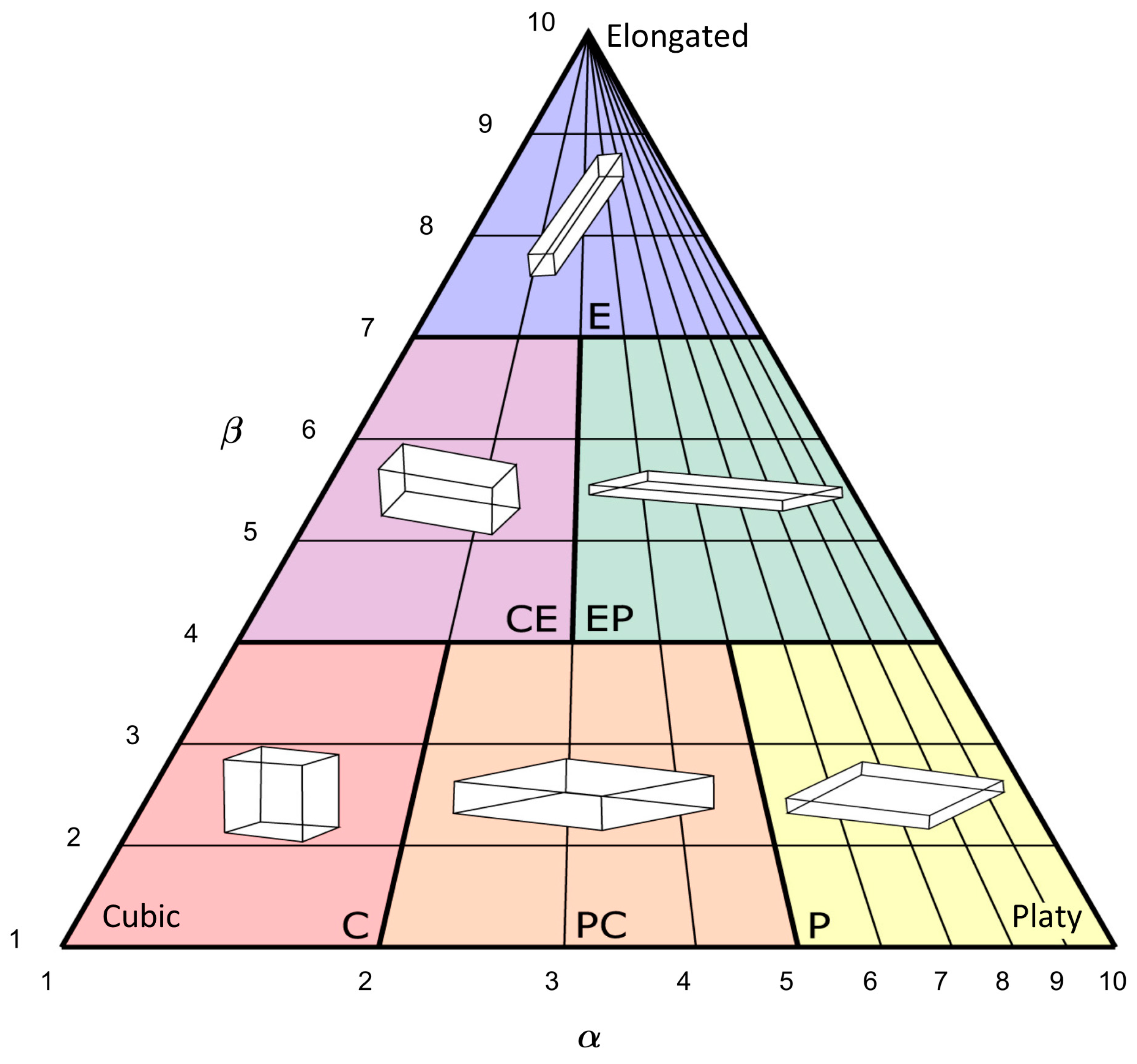
For block shape classification [2], two parameters and were introduced. The parameter , defined by the relationship between the surface area and volume, characterizes the flatness of a block, as shown in Equation (4); the parameter , which quantifies the intervertex co-linearity, distinguishes the elongation of a block. The parameter is associated with a power function of the mean intervertex direction cosine, and only intervertex vectors with chord lengths larger than the median chord length are involved in the calculation.
where is the total surface area of a block, is the average chord length, is the block volume, and and are intervertex vectors.
A triangular graphical representation [2] of BSDD integrated with and was established as shown in Figure 8. Six zones that encompass basic shapes were classified to completely demonstrate the block shape, including C (cubic), E (elongated), P (platy), and three transitional shapes (CE, EP, and PC).
As all vertices, edges and faces of blocks were detected, the block orientation was defined as the orientation of the long axis of a block, namely, the unit vector of the longest intervertex dimension of a block. In case more than one longest intervertex length existed, the block orientation was calculated as the mean orientation from those intervertex vectors. The block orientation is an important factor to formulate a statement for the structure and stiffness of a rock mass [5,63]. The principal BODD of extracted blocks can be determined using the stereographic projection method.
3.6. PCM-SDS: Deriving Fundamental Discontinuity Parameters
Starting from this section, we introduce another simulation-based procedure: the PCM-SDS. The objective of the present step is to acquire the optimal statistics of fundamental discontinuity parameters as input data for DFN simulation.
As the point clusters of all individual discontinuity surfaces are obtained, the orientations can be calculated using their best-fitting planes, and the representative trace lengths can be measured digitally. The orientation and trace length of discontinuity A from Set 1 were calculated as shown in Figure 6c. The orientation results can be plotted in stereographic projection (Figure 9 for Site 1) and the trace network mapping of all sets can then be established. As an example, the trace mapping of Set 1 is shown in Figure 6d. The set spacing was regularly calculated based on the scanline method when conducting conventional surveys. Since each individual discontinuity plane within each set has been constructed in 3D space, a “virtual scanline” can also be introduced to the PCM of the surveyed rock face.
The Kolmogorov–Smirnov (K–S) test [64,65] was employed here to evaluate the fitting degree for probability distributions of orientation, trace length (or radius), and spacing (or density). The best-fitted distributions and representative statistical values can be obtained for DFN modeling in the next step. A summary of the statistical results of Site 1 is tabulated in Table 1.
3.7. PCM-SDS: 3D Stochastic DFN Simulation
Several computer programs have been developed for 3D stochastic DFN simulation and most of them present a good capacity for 3D rock block system realization, such as FracMan [66], 3DEC [67], and UnBlocksgen [68]. The 3DEC was used here due to availability. The geometrical characteristics of discontinuities were adopted as the input properties; a series of discrete, planar, and disc-shaped discontinuities of finite size were created; and then, the cubic-shaped rock mass model was developed for block system generation [2,19,27,69,70].
To ensure a realistic representation of rock blocks, an appropriate size of the simulated model should be evaluated. Kluckner et al. [70] introduced a boundary criterion for model size determination. Kim et al. [69] arranged a virtual borehole extending through the model domain, and the model size was selected based on each discontinuity liner frequency. Macciotta et al. [71] suggested that the model size could be assumed to be approximately four to five times the maximum fragment sizes (e.g., fragmented rockfall block sizes) surveyed in each dimension. Here, the virtual borehole criterion [69] was adapted for determination of the model size. To eliminate border effects, the blocks dissected by the model boundaries were excluded (Figure 10).
3.8. PCM-SDS: Block Extraction and Characterization
As it is possible for any number of realizations to satisfy the statistical criteria imposed, multiple DFN realizations herein were implemented. Kluckner et al. [70] performed several replication tests and proposed 100 replications as a replication factor, which was also adapted to achieve statistically reliable results.
The FISH is an embedded programming language in 3DEC that enables the user to define new functions as needed and interact with and manipulate models. A block extraction program using FISH language was developed, and the vertices, surface areas, and volumes of all blocks for each realization were extracted. Three block indicators of IBSDS, BSDS, and BODS were also acquired following the description in Section 3.5.
4. Results
4.1. Results of the Synthetic Box Model
The synthetic model of the cardboard boxes is an experimental dataset for testing the PCM-DDN extraction method. This model can be regarded as assemblies of three sets of planes. After the calculation, three sets of the box planes were clearly identified as expected, as shown in Figure 11a.
The results showed nine blocks extracted from PCM, as labeled in Figure 11b. The true sizes of boxes have been already measured manually, therefore the relationship between actual sizes and the extracted sizes was precisely assessed. As several boxes were aligned and taped very closely, some blocks were calculated as one large block, such as Block 2. Meanwhile, some boxes were entirely or partially hidden inside (e.g., Block 3) and were absent from the exposed view, therefore only visual sizes were measured and compared. The comparisons are tabulated in Table 2. The maximum deviation is 5.19%, the minimum deviation is 0.30%, and the average deviation is 3.09%. These results reveal an acceptable error.
4.2. Comparison of the Results of Site 1 Using Two Procedures
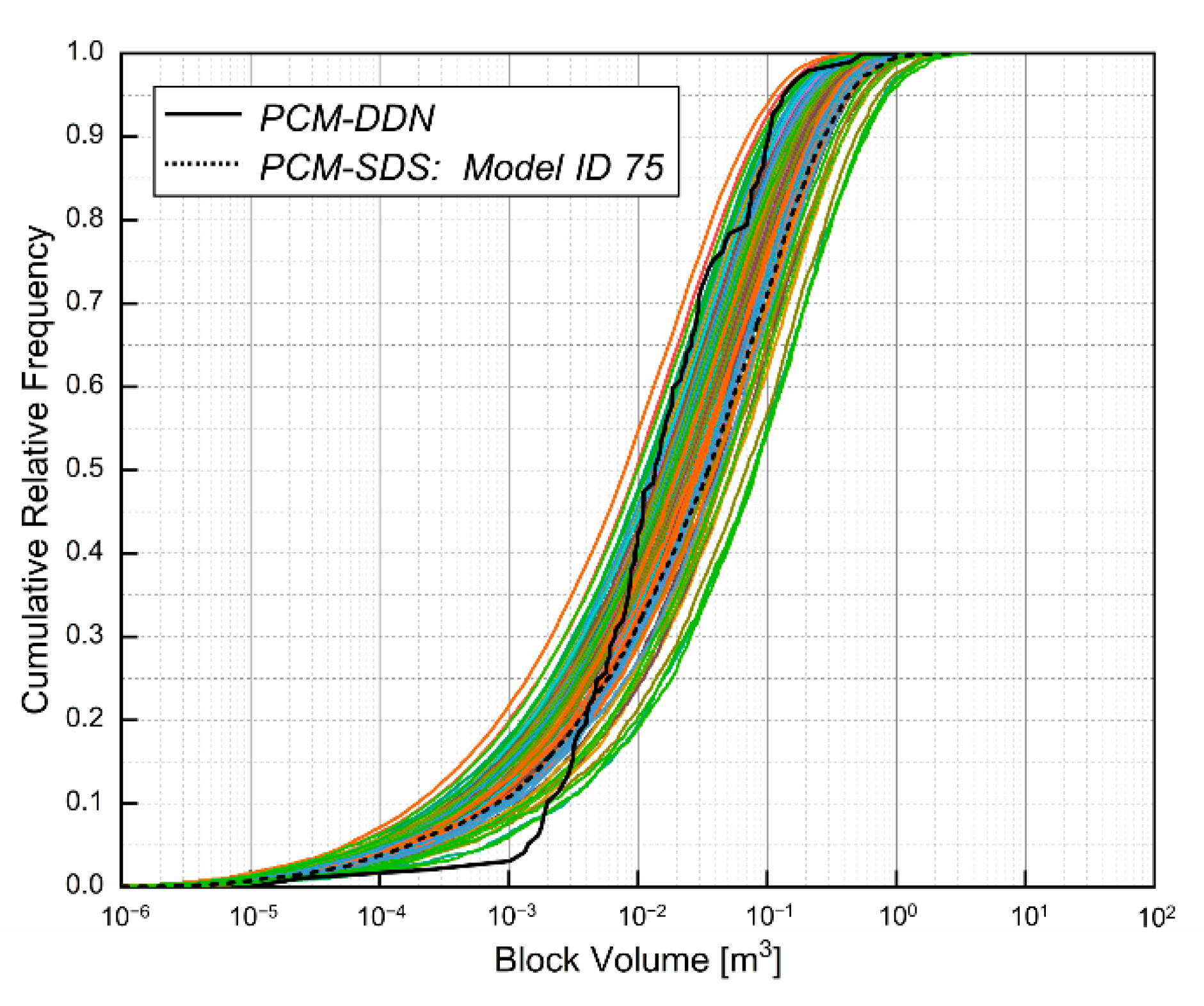
The final block size results obtained from the two procedures (IBSDD and IBSDS) of Site 1 are shown in Figure 12 and Table 3. Model ID 75 from PCM-SDS was selected for comparative analysis. It is apparent that the cumulative distribution curve of IBSDD basically falls in the stripe formed by IBSDS in all simulations. This similarity of the results relies on the well-exposed outcrop in the study area, which verifies the feasibility and validity of the PCM-SDS method. As seen from Table 3, the values of D50 and D75 and the mean block size from IBSDD are less than the values from IBSDS. This discrepancy could be attributed to the limited surveying area where the large blocks are poorly exposed and maintained. The EBSDD of 97 rock blocks extracted from PCM-DDN and their exact locations are presented in Figure 13.
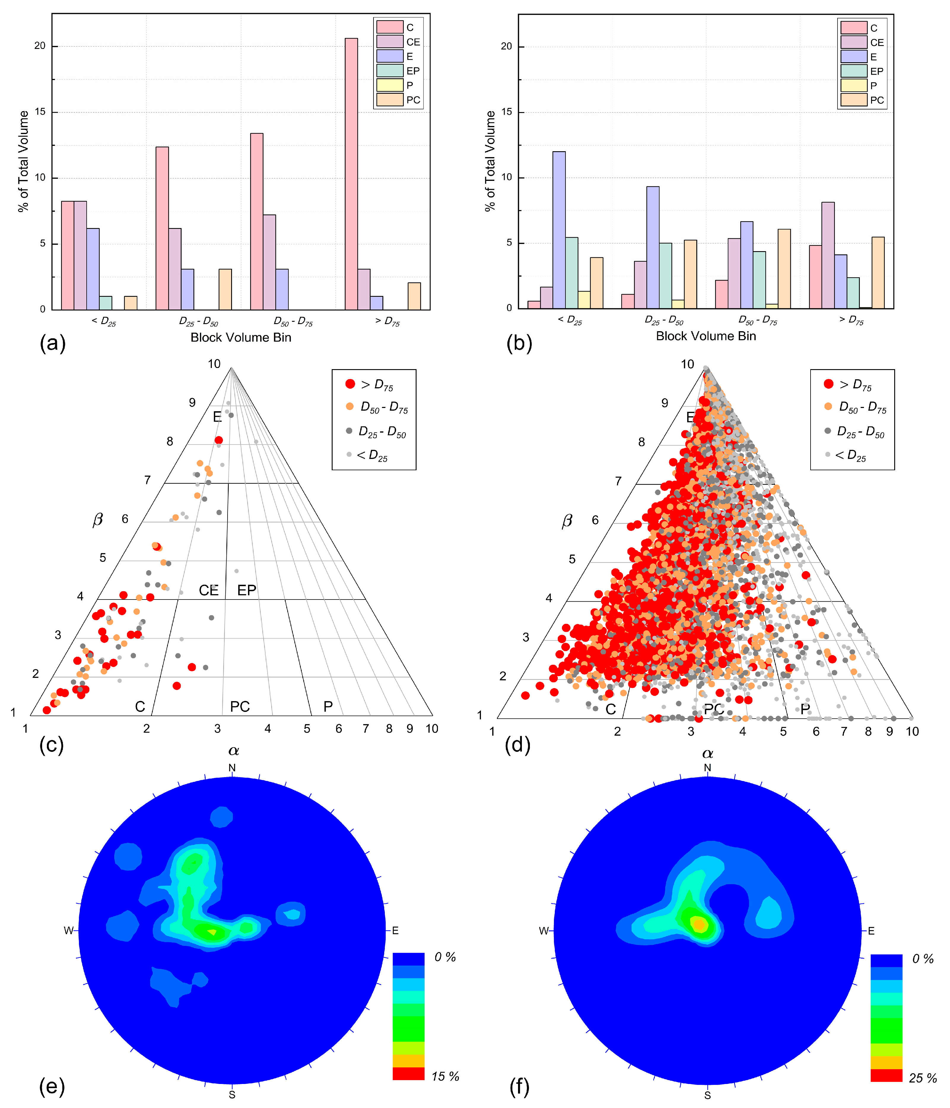
The BSDD and BSDS of model ID 75 are shown in Figure 14c,d. It can be observed that the BSDD and BSDS present similar trends, that is, the main distribution zones are the C, CE, E, and PC sections, which match the field observations well. The BSDS from simulations certainly illustrates an abundant shape presentation, while the smallest blocks range between all block shapes. The difference is that the BSDD is mostly dominated by C and CE shapes (Figure 14a), and the BSDS is mainly composed of E (≤D75, small blocks) and CE (>D75, large blocks) shapes (Figure 14b).
The block orientations from the two procedures (BODD and BODS of model ID 75) are shown in Figure 14e,f, and Table 3. The dominant block orientations (115°/26° from PCM-DDN and 124°/17° from PCM-SDS) are roughly consistent. The major dip directions of blocks are clearly distributed within the range of dip directions of Set 1 (127°/56°) and Set 2 (291°/45°).
Based on the analysis above, the block characterization of Site 1, including size, shape, and orientation from two procedures, yielded a consistent trend. The observed differences are primarily related to the wide disparity in data quantity. The simulated approach (PCM-SDS) is capable of running statistics on blocks with various sizes. In contrast, PCM-DDN excluded considerably small and large blocks that rarely exist on typical exposures.
5. Discussion
5.1. Practical Application of the Proposed Method
An accurate understanding of block geometry is critical in different domains of the rock engineering and mining industry. Typical applications are summarized as follows:
- (1)
- (2)
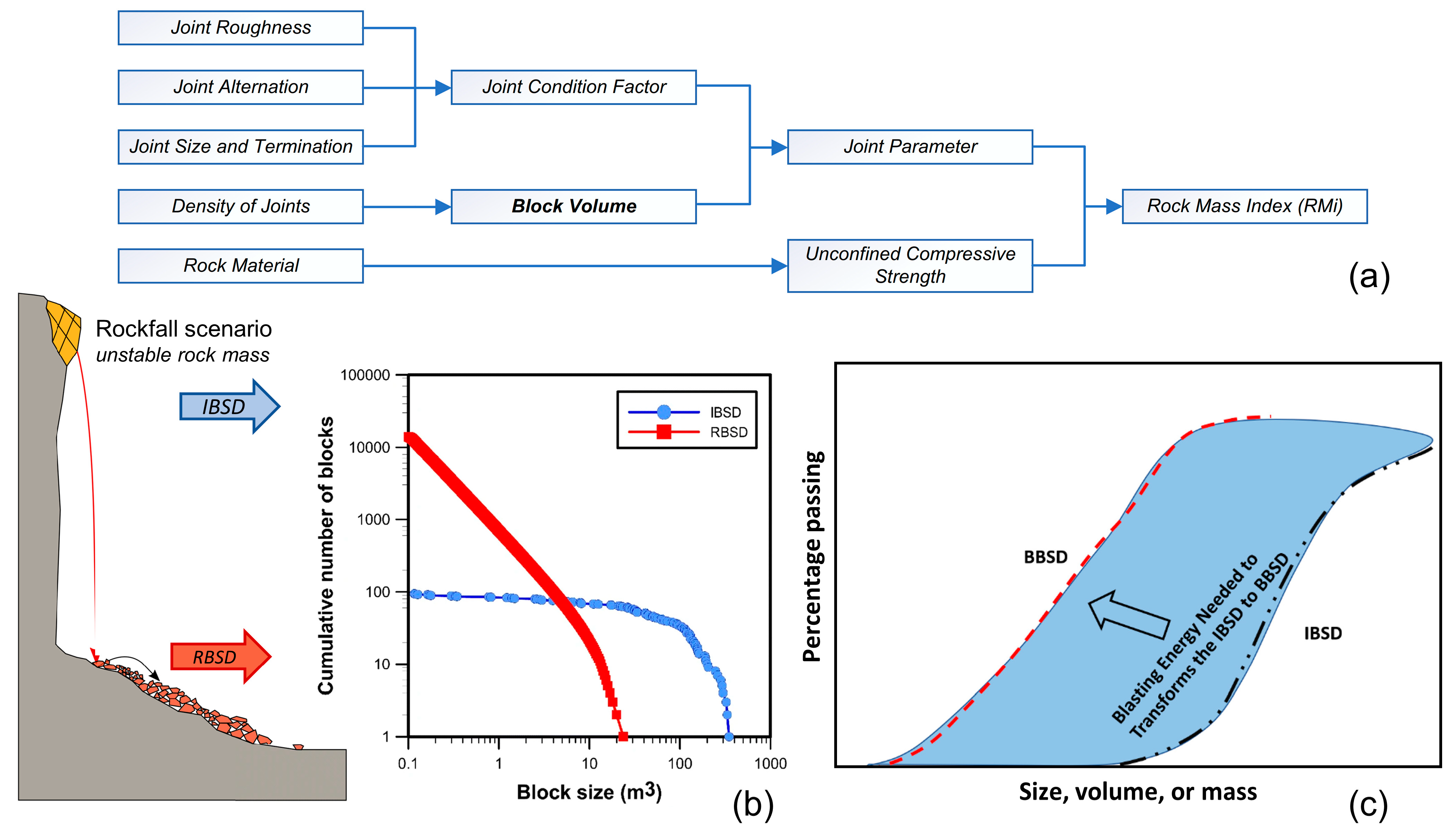
- Blasting design, e.g., explosive consumption and fragmentation energy optimization for mining or tunneling [73]. Taking a quarry project as an example, the IBSD curve and the block shape distribution are important for blasting design and quarry yield prediction. The blasting can be considered as a transformation from IBSD to fragmented size distribution (or blasted block size distribution, BBSD) and the main framework of the energy-block- transition (E-B-T) model can be established [74] (Figure 15c).
- (3)
- (4)
- Stability evaluation and support design of slopes or excavations in jointed rock masses [8].
- (5)
Ruiz-Carulla et al. [78] and Ruiz-Carulla and Corominas [79] established a rockfall fractal fragmentation model (RFFM) for the transformation of the IBSD into the resultant rockfall block size distribution (RBSD). The results from the proposed procedure can be linked to RFFM for simulating impact-induced rock mass fragmentation and disaggregation (Figure 15b).
The applied block shape description delivers not only the mathematical classification of rock blocks but also a statement of the probability of shape distribution. It can also be used in other aspects, such as blast-induced aggregates in quarries or deposited rocks during debris avalanches. When the environment (e.g., the free surface and engineering forces) is known, the block orientation description integrated with block shapes is applicable for rock mass stability analysis. For example, the recumbent platy block is generally prone to sliding failure, while the vertical platy block is more likely to develop broken or toppling failure [9].
It is essential to note that the presently favorable condition of the introduced method is the well-exposed outcrop with discontinuities displayed as planes. The applied algorithms for discontinuity identification mainly aim at extracting the discontinuities exposed as planes, and is not well suited for the linear traces (or cracks) on the rock face. With regard to some slopes at open-pit quarries, where both natural and induced fractures caused by excavation or blast exist, the artificial fractures may be captured as natural surfaces accidently by algorithms. Therefore, manual judgment and supervision are required for clear classification in such circumstances.
The two procedures presented here adopted different paths for the evaluation of block geometry, and the obtained information is complementary. Their relative strengths and weaknesses in relation to various application scenarios are introduced below.
5.1.1. Practical Applicability of PCM-DDN
The results of PCM-DDN are completely dependent on the rock exposure circumstance. The case study of Site 1 supports the view that with a well-exposed surveying area, the results of PCM-DDN can accurately reflect the block characteristics to some extent. However, in practice, it is not easy to find an outcrop containing a fair number of rock blocks with good integrity, which creates difficulties for PCM-DDN to produce a complete and convincing distribution pattern to represent the investigated rock mass.
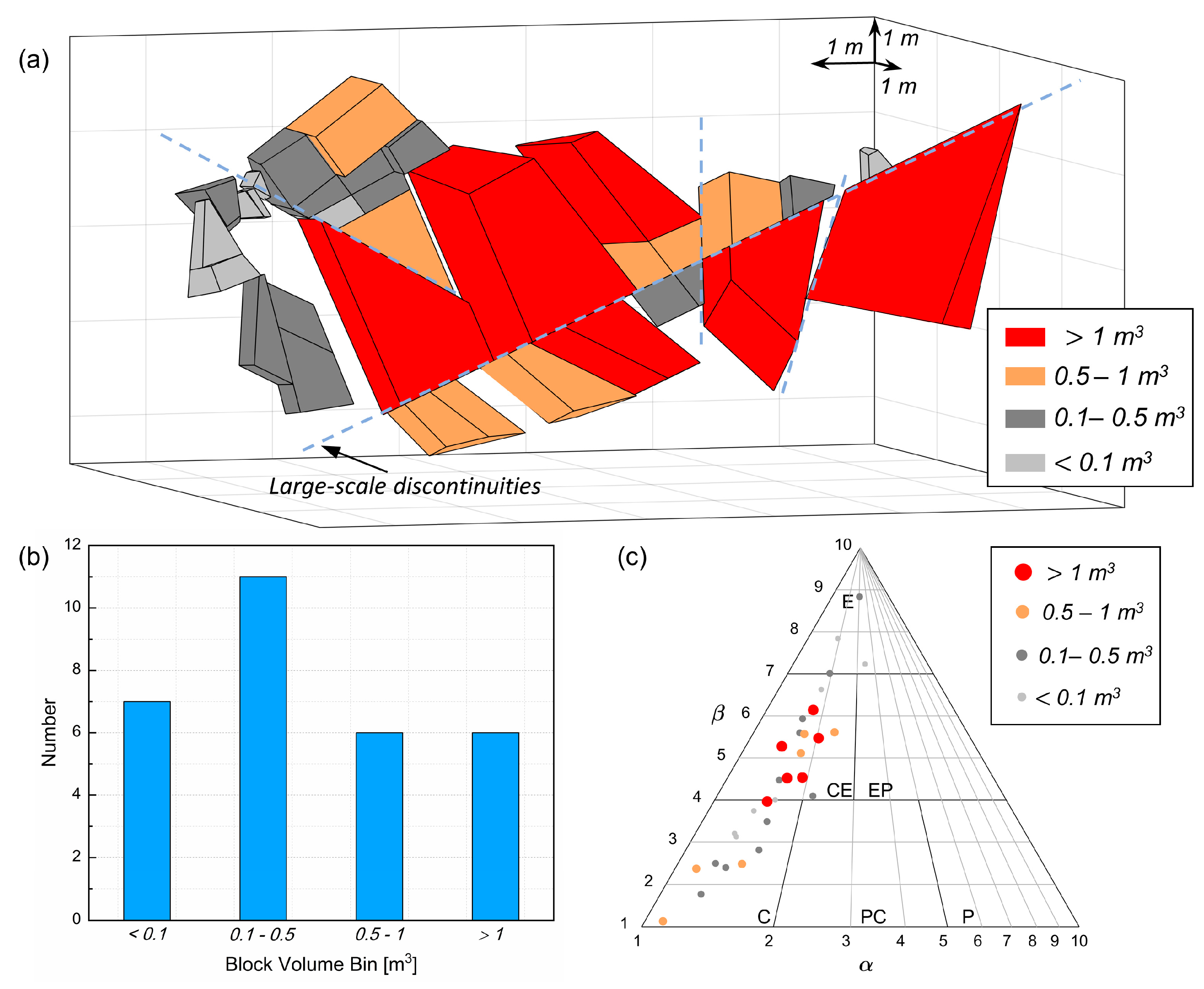
One of the major advantages of this procedure is providing a better means to delineate how various discontinuities are spatially organized for forming blocks and offering the opportunity to locate and characterize the potentially detachable blocks for rockfall hazard research and the associated surface reinforcement strategy. As exemplified in Figure 2b, the near-surface blocks (Figure 16a) of the eastern slope are formed by the main discontinuity network, and after previous rockfall activities, these extracted blocks can be treated as potential rockfall sources for the next time. The average volume is 0.74 m3, and the maximum volume is 5.99 m3 (Figure 16b). The blocks are mainly presented in CE shapes (Figure 16c).
5.1.2. Practical Applicability of PCM-SDS
The accuracy of the stochastic DFN simulation depends on the measurement accuracy of the input parameters. The measurable area of conventional methods (e.g., scanline method or window sampling method) is commonly restricted at the toe of slopes and, therefore, an adequate quantity of measurements cannot be guaranteed for a comprehensive site characterization. PCM-SDS makes it possible to take full advantage of the outcrop space and acquire sufficient discontinuity numbers to ensure statistical stability. Any area of the PCM can be selected as the sampling zone without accessibility-induced restrictions. This full-scale measurement strategy is more reliable and representative of the investigated rock mass than the conventional methods.
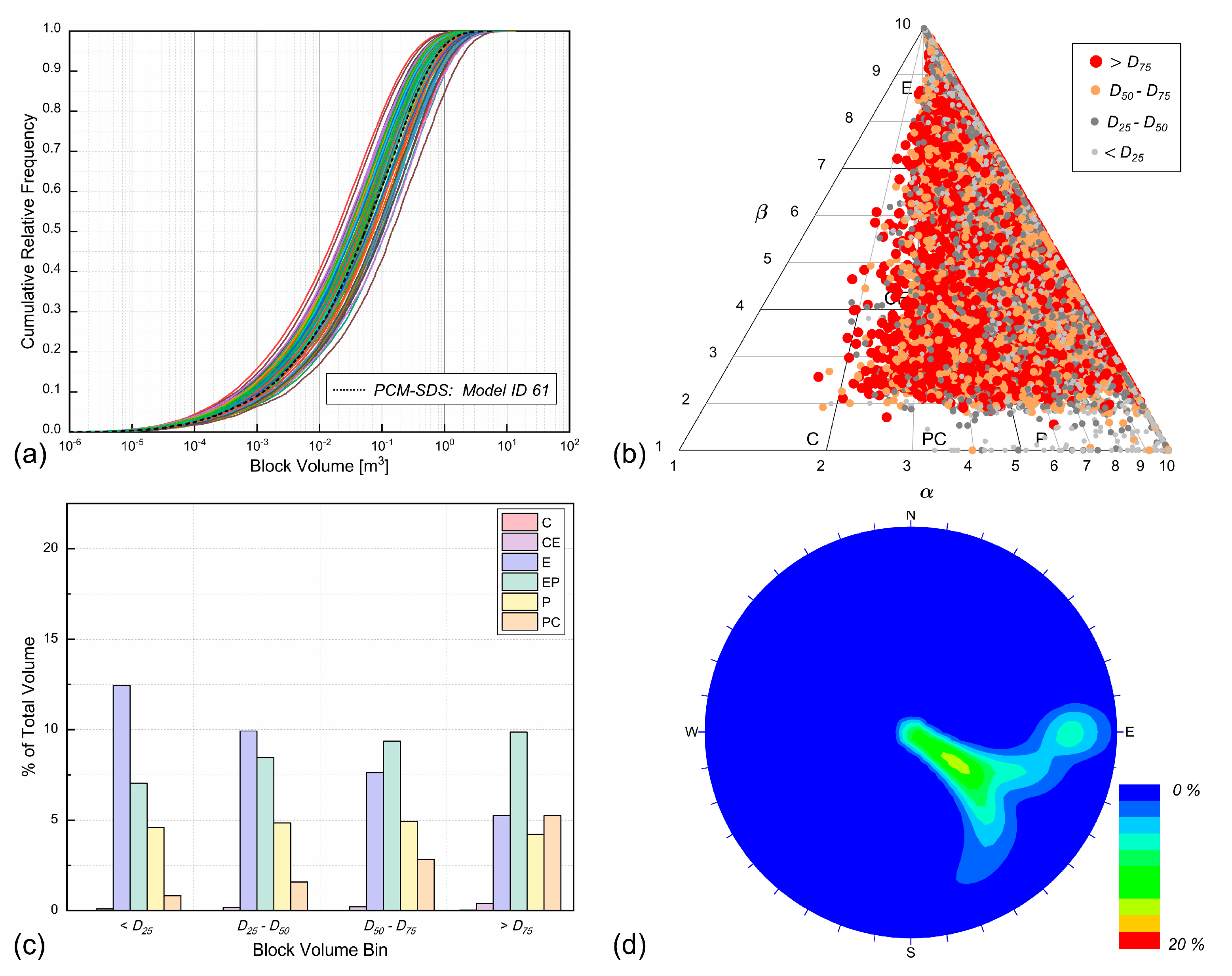
An example of the southern slope of Site 2 is presented in Figure 2c, and the statistical parameters are summarized in Table 4. Using the 3DEC program, 100 realizations of the rock block model are implemented. The resulting IBSDS, as well as BSDS and BODS of model ID 61, are shown in Figure 17 and Table 5. The investigated rock mass is dominated by E, EP and P shape types. The large blocks (>D50) possess more EP shapes, and the small blocks (≤D50) possess more E shapes. As the main block orientation (306°/33°) has a consistent directivity of Set 1 (305°/81°), Set 1 plays a controlling role in the major block shape and orientation of this case.
5.2. Comparison with an Representative Analytical Approach
5.2.1. The Persistence Factor Estimation
The persistence factor is particularly sensitive for block volume estimation when implementing the analytical approach by Cai et al. [26]. In addition, it is the most difficult one to determine among the three parameters, as expressed in Equation (1).
Einstein et al. [80] introduced a rock bridge for persistence calculation, and for a finite sampling length, the persistence factor () can be simply estimated by Equation (6). Currently, there remains a challenging problem with respect to establishing a convenient and reliable measurement procedure for rock bridges and persistence factor determination in field surveys [81]. This is also a reason why unreasonable results may occur when using this analytical approach.
where is the length of the discontinuity and is the length of the rock bridge.
The high-resolution PCM provides a richer perspective for persistence investigation under a 3D environment. To obtain more accurate persistence factor outcomes, the persistence factor was estimated by both field and PCM investigations, and the value range rather than a single value of the persistence factor for one discontinuity set was calculated. The case of the southern slope of Site 2 with three discontinuity sets is suitable for the calculation. Three persistence value ranges (, , ) are tabulated in Table 4.
5.2.2. Comparison with Calculation
The obtained block size indexes (D25, D50, D75 and mean value) from the PCM-SDS of Site 3 were compared with . Applying the product of three persistence values () as the independent variable, the curve was derived. In Figure 18, the D25, D50, D75, and mean value from PCM-SDS with the corresponding shading zone of standard deviation are illustrated. The from the analytical equation is slightly greater than the D75 and mean value from PCM-SDS, and the curve segment is situated at the upper part of the standard deviation zones of D75 and mean value. The difference between and the mean value from PCM-SDS is in the range of 0.015–0.045 m3. This shows a slight overestimation of block size with the equation for this case. The result indicates this empirical equation may not fully reflect the actual influence of the persistence on block size calculation, even the persistence values of all sets are set to 1.
6. Conclusions
Measurements of rock blocks are typically difficult; therefore, their characterization is encumbered with imprecise registrations [3]. Based on the PCM of rock exposure generated from remote sensing techniques, we introduced a consistent and comprehensive method for block characterization with a high level of detail and objectiveness. Two characterization procedures from different perspectives are presented. The first is the PCM-DDN method that presents the existing rock block reconstruction of full-scale rock exposure, in accordance with the mutual intersection relationship of discontinuities. This procedure describes the initial state of rock blocks in detail and reveals the structural complexity of the entire rock surface. The main drawback is that it is uncommon to encounter a well-exposed outcrop containing a fair number of rock blocks with good integrity. The second one, the PCM-SDS method, utilizes a statistically valid representation of discontinuity parameters, and establishes 3D stochastic DFN simulations for block characterization. The digital discontinuity network of rock exposures extracted from PCM can guarantee a sufficient number of measurements and increase the statistical significance of the derived discontinuity parameters compared to conventional methods.
We also developed a multi-dimensional block indicator system, i.e., the block size, shape, orientation, and spatial distribution pattern for systematic and objective block characterization. Three field cases were studied, and the practical feasibilities of the proposed procedures for different application scenarios were discussed, highlighting strengths and limitations. These block indicators are simple and dependable, facilitating easy automation. These indicators demonstrated their potential for related research, such as rock mass quality classification, stability analysis, or blasting design in quarrying and excavation.
Author Contributions
Conceptualization, D.K. and F.W.; methodology, D.K., F.W., and C.S.; software, D.K.; validation, F.W., P.S. and B.L.; formal analysis, B.L.; investigation, D.K., P.S. and B.L.; resources, F.W., C.S. and B.L.; data curation, D.K. and P.S.; writing—original draft preparation, D.K.; writing—review and editing, F.W., C.S. and B.L.; visualization, D.K.; supervision, F.W., C.S. and B.L.; project administration, F.W. and B.L.; funding acquisition, F.W. and B.L. All authors have read and agreed to the published version of the manuscript.
Funding
This research was funded by the National Natural Science Foundation of China (grant nos. 41831290, 42077252) and the Key R&D Project of Zhejiang Province, China (grant no. 2020C03092).
Data Availability Statement
The open-source software VisualSFM for 3D reconstruction by the SfM technique can be found at http://ccwu.me/vsfm/ (accessed on 28 June 2021). The open-source software CloudCompare for PCM pre-processing can be downloaded at https://www.danielgm.net/cc/ (accessed on 28 June 2021). The original codes of fuzzy k-means, DBSCAN and RANSAC algorithms are freely available in the first author’s GitHub repository via https://github.com/snowmanman/PCM (accessed on 28 June 2021). The original code of Nesti-Net algorithm can be found at Dr. Yizhak (Itzik) Ben-Shabat’s GitHub repository via https://github.com/sitzikbs/Nesti-Net (accessed on 28 June 2021). The data file of Site 1 was provided by Dr. Siefko Slob. More details can be found at Dr. Slob’s ResearchGate and his doctoral dissertation at TU Delft, Netherlands.
Acknowledgments
We are grateful for the support and help from Jiangxi Copper Industry Group, Yinshan Mining Industry Co., Ltd.
Conflicts of Interest
The authors declare no conflict of interest.
References
- Priest, S.D. Discontinuity Analysis for Rock Engineering; Chapman & Hall: London, UK, 1993; pp. 219–254. [Google Scholar]
- Kalenchuk, K.S.; Diederichs, M.S.; McKinnon, S. Characterizing block geometry in jointed rockmasses. Int. J. Rock Mech. Min. Sci. 2006, 43, 1212–1225. [Google Scholar] [CrossRef]
- Palmstrom, A. Measurements of and correlations between block size and rock quality designation (RQD). Tunn. Undergr. Sp. Technol. 2005, 20, 362–377. [Google Scholar] [CrossRef]
- Goodman, R.E. Introduction to Rock Mechanics; Wiley: New York, NY, USA, 1989; Volume 2, pp. 221–388. [Google Scholar]
- Buyer, A.; Aichinger, S.; Schubert, W. Applying photogrammetry and semi-automated joint mapping for rock mass characterization. Eng. Geol. 2020, 264, 105332. [Google Scholar] [CrossRef]
- Morelli, G.L. Empirical Assessment of the Mean Block Volume of Rock Masses Intersected by Four Joint Sets. Rock Mech. Rock Eng. 2016, 49, 1759–1771. [Google Scholar] [CrossRef]
- Mavrouli, O.; Corominas, J. Comparing rockfall scar volumes and kinematically detachable rock masses. Eng. Geol. 2017, 219, 64–73. [Google Scholar] [CrossRef]
- Dong, X.; Xu, Q.; Huang, R.; Liu, Q.; Kieffer, D.S. Reconstruction of Surficial Rock Blocks by Means of Rock Structure Modelling of 3D TLS Point Clouds: The 2013 Long-Chang Rockfall. Rock Mech. Rock Eng. 2020, 53, 671–689. [Google Scholar] [CrossRef] [Green Version]
- Goodman, R.; Shi, G. Block Theory and its Application to Rock Engineering; Prentice-Hall: Englewood Cliffs, NJ, USA, 1985. [Google Scholar]
- Sturzenegger, M.; Stead, D.; Elmo, D. Terrestrial remote sensing-based estimation of mean trace length, trace intensity and block size/shape. Eng. Geol. 2011, 119, 96–111. [Google Scholar] [CrossRef]
- Fekete, S.; Diederichs, M. Integration of three-dimensional laser scanning with discontinuum modelling for stability analysis of tunnels in blocky rockmasses. Int. J. Rock Mech. Min. Sci. 2013, 57, 11–23. [Google Scholar] [CrossRef]
- Yao, W.; Mostafa, S.; Yang, Z. Assessment of block size distribution in fractured rock mass and its influence on rock mass mechanical behavior. AIP Adv. 2020, 10, 35124. [Google Scholar] [CrossRef] [Green Version]
- ISRM International society for rock mechanics commission on standardization of laboratory and field tests: Suggested methods for the quantitative description of discontinuities in rock masses. Int. J. Rock Mech. Min. Sci. Geomech. Abstr. 1978, 15, 319–368. [CrossRef]
- Kim, B.H.; Cai, M.; Kaiser, P.K.; Yang, H.S. Estimation of Block Sizes for Rock Masses with Non-persistent Joints. Rock Mech. Rock Eng. 2006, 40, 169. [Google Scholar] [CrossRef]
- Hoek, E.; Carter, T.G.; Diederichs, M.S. Quantification of the Geological Strength Index Chart. In Proceedings of the 47th US Rock Mechanics /Geomechanics Symposium, San Francisco, CA, USA, 23–26 June 2013. [Google Scholar]
- Chen, N.; Kemeny, J.; Jiang, Q.; Pan, Z. Automatic extraction of blocks from 3D point clouds of fractured rock. Comput. Geosci. 2017, 109, 149–161. [Google Scholar] [CrossRef]
- Barton, N.; Lien, R.; Lunde, J. Engineering classification of rock masses for the design of tunnel support. Rock Mech. 1974, 6, 189–236. [Google Scholar] [CrossRef]
- Hardy, A.J.; Ryan, T.M.; Kemeny, J.M. Block size distribution of in situ rock masses using digital image processing of drill core. Int. J. Rock Mech. Min. Sci. 1997, 34, 303–307. [Google Scholar] [CrossRef]
- Lu, P.; Latham, J.-P. Developments in the Assessment of In-situ Block Size Distributions of Rock Masses. Rock Mech. Rock Eng. 1999, 32, 29–49. [Google Scholar] [CrossRef]
- Latham, J.-P.; Van Meulen, J.; Dupray, S. Prediction of in-situ block size distributions with reference to armourstone for breakwaters. Eng. Geol. 2006, 86, 18–36. [Google Scholar] [CrossRef]
- Deere, D.U. Technical description of rock cores for engineering purpose. Felsmech. Ing. 1963, 1, 16–22. [Google Scholar]
- Palmstrom, A. The volumetric joint count―a useful and simple measure of the degree of rock mass jointing. In Proceedings of the 4th International Congress IAEG, New Delhi, India, 10–15 December1982; pp. 221–228. [Google Scholar]
- Palmstrom, A. Characterization of jointing density and the quality of rock masses (in Norwegian). Intern. Rep. Norw. AB Berdal 1974, 26, 3. [Google Scholar]
- Palmström, A.; Singh, R. The deformation modulus of rock masses—Comparisons between in situ tests and indirect estimates. Tunn. Undergr. Sp. Technol. 2001, 16, 115–131. [Google Scholar] [CrossRef]
- Şen, Z.; Eissa, E.A. Rock quality charts for log-normally distributed block sizes. Int. J. Rock Mech. Min. Sci. Geomech. Abstr. 1992, 29, 1–12. [Google Scholar] [CrossRef]
- Cai, M.; Kaiser, P.K.; Uno, H.; Tasaka, Y.; Minami, M. Estimation of rock mass deformation modulus and strength of jointed hard rock masses using the GSI system. Int. J. Rock Mech. Min. Sci. 2004, 41, 3–19. [Google Scholar] [CrossRef]
- Elmouttie, M.K.; Poropat, G. V A Method to Estimate In Situ Block Size Distribution. Rock Mech. Rock Eng. 2012, 45, 401–407. [Google Scholar] [CrossRef]
- Mavrouli, O.; Corominas, J. Evaluation of Maximum Rockfall Dimensions Based on Probabilistic Assessment of the Penetration of the Sliding Planes into the Slope. Rock Mech. Rock Eng. 2020. [Google Scholar] [CrossRef] [Green Version]
- Wang, H.; Latham, J.-P.; Poole, A.B. Predictions of block size distribution for quarrying. Q. J. Eng. Geol. Hydrogeol. 1991, 24, 91–99. [Google Scholar] [CrossRef]
- Saroglou, H.; Marinos, V.; Marinos, P.; Tsiambaos, G. Rockfall hazard and risk assessment: An example from a high promontory at the historical site of Monemvasia, Greece. Nat. Hazards Earth Syst. Sci. 2012, 12, 1823–1836. [Google Scholar] [CrossRef] [Green Version]
- Jern, M. Determination of the In situ Block Size Distribution in Fractured Rock, an Approach for Comparing In-situ Rock with Rock Sieve Analysis. Rock Mech. Rock Eng. 2004, 37, 391–401. [Google Scholar] [CrossRef]
- Stavropoulou, M. Discontinuity frequency and block volume distribution in rock masses. Int. J. Rock Mech. Min. Sci. 2014, 65, 62–74. [Google Scholar] [CrossRef]
- Stavropoulou, M.; Xiroudakis, G. Fracture Frequency and Block Volume Distribution in Rock Masses. Rock Mech. Rock Eng. 2020, 53, 4673–4689. [Google Scholar] [CrossRef]
- Riquelme, A.J.; Abellán, A.; Tomás, R.; Jaboyedoff, M. A new approach for semi-automatic rock mass joints recognition from 3D point clouds. Comput. Geosci. 2014, 68, 38–52. [Google Scholar] [CrossRef] [Green Version]
- Ferrero, A.; Migliazza, M.; Umili, G. Rock mass characterization by means of advanced survey methods. Rock Eng. Rock Mech. Struct. Rock Masses 2014, 17–27. [Google Scholar] [CrossRef]
- Jaboyedoff, M.; Couture, R.; Locat, P. Structural analysis of Turtle Mountain (Alberta) using digital elevation model: Toward a progressive failure. Geomorphology 2009. [Google Scholar] [CrossRef]
- Salvini, R.; Mastrorocco, G.; Esposito, G.; Di Bartolo, S.; Coggan, J.; Vanneschi, C. Use of a remotely piloted aircraft system for hazard assessment in a rocky mining area (Lucca, Italy). Nat. Hazards Earth Syst. Sci. 2018, 18, 287–302. [Google Scholar] [CrossRef] [Green Version]
- Abellán, A.; Oppikofer, T.; Jaboyedoff, M.; Rosser, N.J.; Lim, M.; Lato, M.J. Terrestrial laser scanning of rock slope instabilities. Earth Surf. Process. Landforms 2014, 39, 80–97. [Google Scholar] [CrossRef]
- Abellán, A.; Vilaplana, J.M.; Martínez, J. Application of a long-range Terrestrial Laser Scanner to a detailed rockfall study at Vall de Núria (Eastern Pyrenees, Spain). Eng. Geol. 2006, 88, 136–148. [Google Scholar] [CrossRef]
- Vanhaekendover, H.; Lindenbergh, R.; Ngan-Tillard, D.; Slob, S.; Wezenberg, U. Deterministic in-situ block size estimation using 3D terrestrial laser data. In Proceedings of the ISRM Regional Symposium-EUROCK, Vigo, Spain, 27–29 May 2014. [Google Scholar]
- Mavrouli, O.; Corominas, J.; Jaboyedoff, M. Size Distribution for Potentially Unstable Rock Masses and In Situ Rock Blocks Using LIDAR-Generated Digital Elevation Models. Rock Mech. Rock Eng. 2015, 48, 1589–1604. [Google Scholar] [CrossRef] [Green Version]
- Battulwar, R.; Zare-Naghadehi, M.; Emami, E.; Sattarvand, J. A state-of-the-art review of automated extraction of rock mass discontinuity characteristics using three-dimensional surface models. J. Rock Mech. Geotech. Eng. 2021. [Google Scholar] [CrossRef]
- Slob, S. Automated Rock Mass Characterisation Using 3-D Terrestrial Laser Scanning. Ph.D. Thesis, Technische Universiteit Delft, Delft, The Netherland, 2010. [Google Scholar]
- Wu, F.; Wu, J.; Bao, H.; Li, B.; Shan, Z.; Kong, D. Advances in statistical mechanics of rock masses and its engineering applications. J. Rock Mech. Geotech. Eng. 2021, 13, 22–45. [Google Scholar] [CrossRef]
- Westoby, M.J.; Brasington, J.; Glasser, N.F.; Hambrey, M.J.; Reynolds, J.M. “Structure-from-Motion” photogrammetry: A low-cost, effective tool for geoscience applications. Geomorphology 2012, 179, 300–314. [Google Scholar] [CrossRef] [Green Version]
- Giordan, D.; Adams, M.S.; Aicardi, I.; Alicandro, M.; Allasia, P.; Baldo, M.; De Berardinis, P.; Dominici, D.; Godone, D.; Hobbs, P. The use of unmanned aerial vehicles (UAVs) for engineering geology applications. Bull. Eng. Geol. Environ. 2020, 79, 3437–3481. [Google Scholar] [CrossRef] [Green Version]
- Kong, D.; Saroglou, C.; Wu, F.; Sha, P.; Li, B. Development and application of UAV-SfM photogrammetry for quantitative characterization of rock mass discontinuities. Int. J. Rock Mech. Min. Sci. 2021, 141, 104729. [Google Scholar] [CrossRef]
- Gigli, G.; Casagli, N. Semi-automatic extraction of rock mass structural data from high resolution LIDAR point clouds. Int. J. Rock Mech. Min. Sci. 2011, 48, 187–198. [Google Scholar] [CrossRef]
- Vöge, M.; Lato, M.J.; Diederichs, M.S. Automated rockmass discontinuity mapping from 3-dimensional surface data. Eng. Geol. 2013, 164, 155–162. [Google Scholar] [CrossRef]
- Lato, M.; Diederichs, M.S.; Hutchinson, D.J.; Harrap, R. Optimization of LiDAR scanning and processing for automated structural evaluation of discontinuities in rockmasses. Int. J. Rock Mech. Min. Sci. 2009, 46, 194–199. [Google Scholar] [CrossRef]
- Kong, D.; Wu, F.; Saroglou, C. Automatic identification and characterization of discontinuities in rock masses from 3D point clouds. Eng. Geol. 2020. [Google Scholar] [CrossRef]
- Li, X.; Chen, J.; Zhu, H. A new method for automated discontinuity trace mapping on rock mass 3D surface model. Comput. Geosci. 2016, 89, 118–131. [Google Scholar] [CrossRef]
- Ben-Shabat, Y.; Lindenbaum, M.; Fischer, A. Nesti-net: Normal estimation for unstructured 3d point clouds using convolutional neural networks. In Proceedings of the IEEE Conference on Computer Vision and Pattern Recognition, Long Beach, CA, USA, 16–20 June 2019. [Google Scholar]
- Ben-Shabat, Y.; Lindenbaum, M.; Fischer, A. 3DmFV: Three-Dimensional Point Cloud Classification in Real-Time Using Convolutional Neural Networks. IEEE Robot. Autom. Lett. 2018, 3, 3145–3152. [Google Scholar] [CrossRef]
- Liu, Q.; Kaufmann, V. Integrated Assessment of Cliff Rockfall Hazards by Means of Rock Structure Modelling Applied to TLS data: New Developments. In Proceedings of the ISRM Regional Symposium—EUROCK, Salzburg, Austria, 7–10 October 2015. [Google Scholar]
- Bezdek, J.C. Pattern Recognition with Fuzzy Objective Function Algorithms; Springer: New York, NY, USA, 1981; ISBN 147570450X. [Google Scholar]
- Hammah, R.E.; Curran, J.H. On distance measures for the fuzzy K-means algorithm for joint data. Rock Mech. Rock Eng. 1999, 32, 1–27. [Google Scholar] [CrossRef]
- Schubert, E.; Sander, J.; Ester, M.; Kriegel, H.P.; Xu, X. DBSCAN revisited, revisited: Why and how you should (still) use DBSCAN. ACM Trans. Database Syst. 2017, 42, 1–21. [Google Scholar] [CrossRef]
- Ester, M.; Kriegel, H.-P.; Sander, J.; Xu, X. A Density-Based Algorithm for Discovering Clusters in Large Spatial Databases with Noise. In Proceedings of the 2nd International Conference on Knowledge Discovery and Data Mining, Portland, OR, USA, 2–4 August 1996. [Google Scholar]
- Zhu, Y.; Ting, K.M.; Carman, M.J. Density-ratio based clustering for discovering clusters with varying densities. Pattern Recognit. 2016, 60, 983–997. [Google Scholar] [CrossRef]
- Tonini, M.; Abellan, A. Rockfall detection from terrestrial LiDAR point clouds: A clustering approach using R. J. Spat. Inf. Sci. 2014. [Google Scholar] [CrossRef]
- Fischler, M.A.; Bolles, R.C. Random sample consensus: A Paradigm for Model Fitting with Applications to Image Analysis and Automated Cartography. Commun. ACM 1981, 24, 381–395. [Google Scholar] [CrossRef]
- Gottsbacher, L.K.J. Calculation of the Young’s Modulus for Rock Masses with 3DEC and Comparing It with Empirical Methods. Master’s Thesis, Graz University of Technology, Graz, Austria, 2017. [Google Scholar]
- Massey, F.J. The Kolmogorov-Smirnov Test for Goodness of Fit. J. Am. Stat. Assoc. 1951, 46, 68–78. [Google Scholar] [CrossRef]
- Umili, G.; Bonetto, S.M.R.; Mosca, P.; Vagnon, F.; Ferrero, A.M. In Situ Block Size Distribution Aimed at the Choice of the Design Block for Rockfall Barriers Design: A Case Study along Gardesana Road. Geosciences 2020, 10, 223. [Google Scholar] [CrossRef]
- Golder Associates. FracMan Software. Available online: https://www.golder.com/fracman/ (accessed on 28 June 2021).
- Itasca Consulting Group Inc. 3DEC Software. Available online: https://www.itascacg.com/software/3dec (accessed on 28 June 2021).
- Rasmussen, L.L. UnBlocksgen: A Python library for 3D rock mass generation and analysis. SoftwareX 2020, 12, 100577. [Google Scholar] [CrossRef]
- Kim, B.-H.; Peterson, R.L.; Katsaga, T.; Pierce, M.E. Estimation of rock block size distribution for determination of Geological Strength Index (GSI) using discrete fracture networks (DFNs). Min. Technol. 2015, 124, 203–211. [Google Scholar] [CrossRef]
- Kluckner, A.; Söllner, P.; Schubert, W.; Pötsch, M. Estimation of the in situ Block Size in Jointed Rock Masses using Three-Dimensional Block Simulations and Discontinuity Measurements. In Proceedings of the 13th ISRM International Congress of Rock Mechanics, Montreal, Canada, 10–13 May 2015. [Google Scholar]
- Macciotta, R.; Gräpel, C.; Skirrow, R. Fragmented rockfall volume distribution from photogrammetry-based structural mapping and discrete fracture networks. Appl. Sci. 2020, 10, 6977. [Google Scholar] [CrossRef]
- Yarahmadi, R.; Bagherpour, R.; Taherian, S.-G.; Sousa, L.M.O. Discontinuity modelling and rock block geometry identification to optimize production in dimension stone quarries. Eng. Geol. 2018, 232, 22–33. [Google Scholar] [CrossRef]
- Latham, J.-P.; Lu, P. Development of an assessment system for the blastability of rock masses. Int. J. Rock Mech. Min. Sci. 1999, 36, 41–55. [Google Scholar] [CrossRef]
- Salmi, E.F.; Sellers, E.J. A review of the methods to incorporate the geological and geotechnical characteristics of rock masses in blastability assessments for selective blast design. Eng. Geol. 2021, 281, 105970. [Google Scholar] [CrossRef]
- Palmstrøm, A. Characterizing rock masses by the RMi for use in practical rock engineering: Part 1: The development of the Rock Mass index (RMi). Tunn. Undergr. Sp. Technol. 1996, 11, 175–188. [Google Scholar] [CrossRef]
- Rives, T.; Razack, M.; Petit, J.-P.; Rawnsley, K.D. Joint spacing: Analogue and numerical simulations. J. Struct. Geol. 1992, 14, 925–937. [Google Scholar] [CrossRef]
- Laughton, C.; Nelson, P.P. The Development of Rock Mass Parameters For Use In the Prediction of Tunnel Boring Machine Performance. In Proceedings of the ISRM International Symposium—EUROCK 96, Turin, Italy, 2–5 September 1996. [Google Scholar]
- Ruiz-Carulla, R.; Corominas, J.; Mavrouli, O. A fractal fragmentation model for rockfalls. Landslides 2017, 14, 875–889. [Google Scholar] [CrossRef]
- Ruiz-Carulla, R.; Corominas, J. Analysis of Rockfalls by Means of a Fractal Fragmentation Model. Rock Mech. Rock Eng. 2020, 53, 1433–1455. [Google Scholar] [CrossRef]
- Einstein, H.H.; Veneziano, D.; Baecher, G.B.; O’Reilly, K.J. The effect of discontinuity persistence on rock slope stability. Int. J. Rock Mech. Min. Sci. Geomech. Abstr. 1983, 20, 227–236. [Google Scholar] [CrossRef]
- Elmo, D.; Donati, D.; Stead, D. Challenges in the characterisation of intact rock bridges in rock slopes. Eng. Geol. 2018, 245, 81–96. [Google Scholar] [CrossRef]
Figure 1.
The surveyed rock exposure of Site 1 [43]. A partial magnification of two blocks is demonstrated, and some interrelated discontinuities are marked. The two white boards are 60 by 60 cm in dimension, and act as supplementary scale and orientation reference markers during the analysis of the laser scanned point cloud data. View direction is towards the East.

Figure 2.
(a) Site map of Yinshan open-pit copper mine extracted from Google Earth. (b) Orthophoto of the eastern slope generated from UAV photogrammetry. (c) Orthophoto of the southern slope generated from UAV photogrammetry.
Figure 2.
(a) Site map of Yinshan open-pit copper mine extracted from Google Earth. (b) Orthophoto of the eastern slope generated from UAV photogrammetry. (c) Orthophoto of the southern slope generated from UAV photogrammetry.

Figure 3.
(a) Scanned cardboard boxes for experimental study; (b) 3D PCM of boxes.

Figure 4.
Flow chart of the proposed method.

Figure 5.
Scheme of normal vector estimation based on Nesti-Net algorithm updated from Ben-Shabat et al. [53]. The multi-scale point statistics for each point from a given PCM is computed. Then, the optimal scale is determined by a scale manager network. The normal vectors are calculated by mixture-of-experts CNN, and mapped by a HSV-rendering technique (Liu and Kaufmann [55]).

Figure 6.
(a) Discontinuity set assignment to each point of Site 1 using different colors. (b) Each individual discontinuity of Set 1 is separated and delineated using different colors. (c) One example of parameters calculated for discontinuity A: orientation, trace length, and fitting plane equation. (d) Digital trace mapping of Set 1.

Figure 7.
The discontinuity collections of Blocks 1 (a) and 2 (d), the polyhedral modeling based on extension of existing discontinuity planes of Blocks 1 (b) and 2 (e), and the final block model and calculated parameters for Blocks 1 (c) and 2 (f).
Figure 7.
The discontinuity collections of Blocks 1 (a) and 2 (d), the polyhedral modeling based on extension of existing discontinuity planes of Blocks 1 (b) and 2 (e), and the final block model and calculated parameters for Blocks 1 (c) and 2 (f).

Figure 8.
Block shape classification diagram based on the parameters and .

Figure 9.
The orientation results for Site 1 in the stereographic projection (i.e., equal angle net on the lower hemisphere).
Figure 9.
The orientation results for Site 1 in the stereographic projection (i.e., equal angle net on the lower hemisphere).

Figure 10.
Three-dimensional (3D) rock block model based on the stochastic DFN simulation before and after excluding the boundary blocks.
Figure 10.
Three-dimensional (3D) rock block model based on the stochastic DFN simulation before and after excluding the boundary blocks.

Figure 11.
(a) The stereographic projection of three sets of planes (i.e., equal angle net on the lower hemisphere). (b) The extraction of blocks of the synthetic box model with all blocks labeled.
Figure 11.
(a) The stereographic projection of three sets of planes (i.e., equal angle net on the lower hemisphere). (b) The extraction of blocks of the synthetic box model with all blocks labeled.

Figure 12.
The block volume distribution of IBSDD and IBSDS. All color curves represent IBSDS from PCM-SDS of all simulated models.
Figure 12.
The block volume distribution of IBSDD and IBSDS. All color curves represent IBSDS from PCM-SDS of all simulated models.

Figure 13.
The EBSDD of rock blocks extracted from PCM-DDN of Site 1.

Figure 14.
The shape distribution and block volume ranges obtained from PCM-DDN (a) and PCM-SDS (b) for Site 1. The block shape distribution from PCM-DDN (c) and PCM-SDS (d) for Site 1. The block orientation distribution from PCM-DDN (e) and PCM-SDS (f) for Site 1.
Figure 14.
The shape distribution and block volume ranges obtained from PCM-DDN (a) and PCM-SDS (b) for Site 1. The block shape distribution from PCM-DDN (c) and PCM-SDS (d) for Site 1. The block orientation distribution from PCM-DDN (e) and PCM-SDS (f) for Site 1.

Figure 15.
(a) The main inherent rock mass parameters in the RMi according to [75]. (b) A schematic view of the RFFM. The change in block volume distribution by fragmentation. The IBSD results in an increase of the number of blocks by fragmentation (RBSD) modified from Ruiz-Carulla and Corominas [79]. (c) Schematic view of the energy-block-transition model modified from Salmi and Sellers [74].

Figure 16.
(a) The EBSDD of rock blocks extracted from PCM-DDN. (b) The block volume distribution of extracted rock blocks. (c) The block shape distribution from PCM-DDN.
Figure 16.
(a) The EBSDD of rock blocks extracted from PCM-DDN. (b) The block volume distribution of extracted rock blocks. (c) The block shape distribution from PCM-DDN.

Figure 17.
(a) The block volume distribution of IBSDS from PCM-SDS of all simulated models. (b) The block shape distribution from PCM-SDS. (c) The corresponding shape distribution with block volume ranges. (d) The block orientation distribution from PCM-SDS.
Figure 17.
(a) The block volume distribution of IBSDS from PCM-SDS of all simulated models. (b) The block shape distribution from PCM-SDS. (c) The corresponding shape distribution with block volume ranges. (d) The block orientation distribution from PCM-SDS.

Figure 18.
The relation between and from the analytical approach by Cai et al. [26]. The D25, D50, D75, and mean value from PCM-SDS with the corresponding shading zone of the standard deviation are also illustrated.
Figure 18.
The relation between and from the analytical approach by Cai et al. [26]. The D25, D50, D75, and mean value from PCM-SDS with the corresponding shading zone of the standard deviation are also illustrated.


Table 1.
Summary of the statistical parameters of Site 1 identified from PCM.
| Set | Orientation (°) | Trace Length (m) | Normal Set Spacing (m) | ||||
|---|---|---|---|---|---|---|---|
| Fisher Distribution | Log Normal Distribution | Log Normal Distribution | |||||
| Dip Dir | Dip | Mean | Standard Deviation | Mean | Standard Deviation | ||
| Set 1 | 127 | 56 | 15.17 | 0.27 | 0.135 | 0.34 | 0.016 |
| Set 2 | 291 | 45 | 35.09 | 0.55 | 0.304 | 0.15 | 0.067 |
| Set 3 | 227 | 83 | 34.89 | 0.45 | 0.386 | 0.25 | 0.061 |
| Set 4 | 279 | 81 | 37.96 | 0.44 | 0.107 | 0.18 | 0.119 |
Table 2.
Comparison results between extracted block sizes and manually measured sizes.
| Block ID | Manually Measured Size (m3) | Extracted Size (m3) | Percent Deviation |
|---|---|---|---|
| 1 | 0.2160 | 0.2111 | 2.27% |
| 2 | 0.4320 | 0.4307 | 0.30% |
| 3 | 0.0689 | 0.0701 | 1.74% |
| 4 | 0.3645 | 0.3780 | 3.70% |
| 5 | 0.0506 | 0.0531 | 4.94% |
| 6 | 0.0540 | 0.0561 | 3.89% |
| 7 | 0.0630 | 0.0642 | 1.90% |
| 8 | 0.0180 | 0.0187 | 3.89% |
| 9 | 0.0270 | 0.0284 | 5.19% |
Table 3.
Summary of block characterization results of Site 1 acquired from two procedures.
| Method | Block Size (m3) | Block Orientation (Dip Dir/Dip, °) | |||
|---|---|---|---|---|---|
| D25 | D50 | D75 | Mean | ||
| PCM-DDN | 0.005 | 0.014 | 0.038 | 0.041 | 115/26 |
| PCM-SDS: Model ID 75 | 0.006 | 0.035 | 0.120 | 0.101 | 124/17 |
| PCM-SDS: All models 1 | M: 0.005 | M: 0.027 | M: 0.092 | M: 0.084 | -- |
| SD: 0.003 | SD: 0.014 | SD: 0.044 | SD: 0.060 | ||
1 M: mean value; SD, standard deviation.
Table 4.
Summary of the statistical parameters of Site 2 identified from PCM of the southern slope.
| Set | Orientation (°) | Trace Length (m) | Normal Set Spacing (m) | Persistence Factor | ||||
|---|---|---|---|---|---|---|---|---|
| Fisher Distribution | Log Normal Distribution | Log Normal Distribution | -- | |||||
| Dip Dir | Dip | Mean | Standard Deviation | Mean | Standard Deviation | Value Range | ||
| Set 1 | 305 | 81 | 93.76 | 1.14 | 0.601 | 0.25 | 0.069 | 85–100% |
| Set 2 | 6 | 76 | 99.60 | 1.52 | 0.862 | 0.61 | 0.240 | 85–100% |
| Set 3 | 108 | 42 | 273.68 | 1.52 | 1.183 | 0.745 | 0.387 | 90–100% |
Table 5.
Summary of block characterization results of Site 2 acquired from PCM-SDS of the southern slope.
Table 5.
Summary of block characterization results of Site 2 acquired from PCM-SDS of the southern slope.
| Method | Block Size (m3) | Block Orientation (Dip dir/Dip, °) | |||
|---|---|---|---|---|---|
| D25 | D50 | D75 | Mean | ||
| PCM-SDS: Model ID 61 | 0.009 | 0.053 | 0.212 | 0.192 | 306/33 |
| PCM-SDS: All models 1 | M: 0.008 | M: 0.051 | M: 0.196 | M: 0.179 | -- |
| SD: 0.004 | SD: 0.025 | SD: 0.092 | SD: 0.079 | ||
1 M: mean value; SD, standard deviation.
Publisher’s Note: MDPI stays neutral with regard to jurisdictional claims in published maps and institutional affiliations. |
© 2021 by the authors. Licensee MDPI, Basel, Switzerland. This article is an open access article distributed under the terms and conditions of the Creative Commons Attribution (CC BY) license (https://creativecommons.org/licenses/by/4.0/).
Share and Cite
MDPI and ACS Style
Kong, D.; Wu, F.; Saroglou, C.; Sha, P.; Li, B. In-Situ Block Characterization of Jointed Rock Exposures Based on a 3D Point Cloud Model. Remote Sens. 2021, 13, 2540. https://0-doi-org.brum.beds.ac.uk/10.3390/rs13132540
AMA Style
Kong D, Wu F, Saroglou C, Sha P, Li B. In-Situ Block Characterization of Jointed Rock Exposures Based on a 3D Point Cloud Model. Remote Sensing. 2021; 13(13):2540. https://0-doi-org.brum.beds.ac.uk/10.3390/rs13132540
Chicago/Turabian StyleKong, Deheng, Faquan Wu, Charalampos Saroglou, Peng Sha, and Bo Li. 2021. "In-Situ Block Characterization of Jointed Rock Exposures Based on a 3D Point Cloud Model" Remote Sensing 13, no. 13: 2540. https://0-doi-org.brum.beds.ac.uk/10.3390/rs13132540
Note that from the first issue of 2016, this journal uses article numbers instead of page numbers. See further details here.