Can Vegetation Indices Serve as Proxies for Potential Sun-Induced Fluorescence (SIF)? A Fuzzy Simulation Approach on Airborne Imaging Spectroscopy Data

Abstract

In this study, we are testing a proxy for red and far-red Sun-induced fluorescence (SIF) using an integrated fuzzy logic modelling approach, termed as SIF_fuzzy and SIF_fuzzy-APAR. The SIF emitted from the core of the photosynthesis and observed at the top-of-canopy is regulated by three major controlling factors: (1) light interception and absorption by canopy plant cover; (2) escape fraction of SIF photons (fesc); (3) light use efficiency and non-photochemical quenching (NPQ) processes. In our study, we proposed and validated a fuzzy logic modelling approach that uses different combinations of spectral vegetation indices (SVIs) reflecting such controlling factors to approximate the potential SIF signals at 760 nm and 687 nm. The HyPlant derived and field validated SVIs (i.e., SR, NDVI, EVI, NDVIre, PRI) have been processed through the membership transformation in the first stage, and in the next stage the membership transformed maps have been processed through the Fuzzy Gamma simulation to calculate the SIF_fuzzy. To test whether the inclusion of absorbed photosynthetic active radiation (APAR) increases the accuracy of the model, the SIF_fuzzy was multiplied by APAR (SIF_fuzzy-APAR). The agreement between the modelled SIF_fuzzy and actual SIF airborne retrievals expressed by R² ranged from 0.38 to 0.69 for SIF₇₆₀ and from 0.85 to 0.92 for SIF₆₈₇. The inclusion of APAR improved the R² value between SIF_fuzzy-APAR and actual SIF. This study showed, for the first time, that a diverse set of SVIs considered as proxies of different vegetation traits, such as biochemical, structural, and functional, can be successfully combined to work as a first-order proxy of SIF. The previous studies mainly included the far-red SIF whereas, in this study, we have also focused on red SIF along with far-red SIF. The analysis carried out at 1 m spatial resolution permits to better infer SIF behaviour at an ecosystem-relevant scale.

1. Introduction

Sun-induced fluorescence (SIF) has emerged as a promising remote sensing (RS) signal in the contemporary era to understand and monitor the terrestrial vegetation activity as well as their structural and functional diversity [1,2,3,4]. The potential of SIF has been well recognized by scientists and research communities because of its direct link to plant photosynthetic activity and plant conditions [5]. Due to a strong relation of chlorophyll fluorescence with photosynthesis, the SIF as a product of chlorophyll fluorescence was observed to indicate the gross primary productivity (GPP) under the clear sky as reported by several studies [6,7,8,9,10]. However, the SIF signal is very weak in comparison to reflected solar energy as only a small fraction of the absorbed energy is re-emitted in the form of SIF [11,12]. The SIF signal is influenced by three main factors which may impact the accuracy of SIF estimation at the canopy level: (1) light interception or light absorption by canopy plant cover, expressed by absorbed photosynthetic active radiation (APAR). APAR can be influenced by several vegetation traits, such as fractional cover, leaf chlorophyll content, leaf angle distribution, leaf clumping, etc. [13], indicating the dependence of SIF on vegetation traits; (2) SIF reabsorption and scattering—most of the photons emitted by plants are reabsorbed or scattered within the canopy [12,14,15], therefore, the fluorescence signal is dependent on the escape fraction of SIF (fesc) which may vary for different vegetation; (3) the light use efficiency (LUE)—absorbed light used for photosynthesis has a strong impact on the functional/physiological regulation of the leaf which is highly dynamic [16]. The relation between the efficiency of leaf photosynthesis and the intensity of SIF is non-linear as it is controlled by three different paths of energy use/dissipation, i.e., photosynthetic electron flow, non-photochemical quenching (NPQ) and fluorescence emission [17].

The traditional RS of vegetation solely relies on the canopy reflectance at different spectral channels and has been widely applied and implemented for several ecosystem applications such as croplands [18,19,20], grasslands [21], peatlands [22,23], etc. Over the past few decades, vegetation monitoring based on spectral vegetation indices (SVIs) have been used to interpret the canopy greenness [24,25], biomass [26,27], water content [28,29,30], leaf area [31,32], zeaxanthin content [33,34], etc. and have greatly enhanced our understanding of the terrestrial vegetation [35]. However, most of the remotely sensed SVIs alone are not sensitive enough to capture the short-term dynamic (i.e., hourly) changes in the photosynthetic process caused by different environmental conditions (i.e., incident irradiance) or stress factors impacting plant physiology [36].

Bandopadhyay et al. [1] have shown that single spectral vegetation indices (SVIs) individually, although related to SIFs, cannot be used to approximate SIF signals with good accuracy. On the other hand, some of the above factors influencing SIF can be reflected by different SVIs, therefore we hypothesized that SIF can be approximated by the combination of different SVIs. The SVIs like Normalized Difference Vegetation Index (NDVI) and Simple Ratio (SR), which successively improved our understanding of vegetation greenness content and plant phenology, can approximate the SIF signals up to a certain limit evident by the positive agreements in several studies [1,37]. These two indices developed from the canopy reflectance spectra obtained for the region of red and NIR are significantly influenced by the canopy structure, light use absorption and light interception, canopy chemical contents, and photosynthetic activity [38]. Such properties of NDVI and SR connect them with the factors related to light absorption and to some extent with fesc of SIF emission, which can only be able to approximate the SIF signal up to a certain limit. Similarly, Enhanced Vegetation Index (EVI) is an optimized spectral index sensitive to light absorption. Although EVI and NDVI both are highly sensitive to the canopy biomass content, NDVI saturates under high biomass and is unable to replicate the actual biomass content of the vegetation [39]. Therefore, EVI can more closely be related to fesc in comparison to NDVI and SR and may help in the estimation of SIF. The red-edge-based normalized difference vegetation index (NDVIre) indicates the transition boundary between the red and NIR region disentangles the absorption by chlorophyll in the red visible region and scattering due to leaf internal structure in the NIR region [21,40]. It denotes that NDVIre is influenced by the leaf absorption content and canopy structure that have a direct connection with the SIF emission and fesc. The narrowband Photochemical Reflectance Index (PRI) indicates the NPQ process and plant xanthophyll cycles which are highly dynamic with environmental factors [41,42]. This NPQ process is parallelly working with photochemical quenching and chlorophyll fluorescence and significantly improves our understanding of SIF emission in line of the argument of the third factor controlling SIF [42]. Although all such SVIs have a certain relation with the SIF, evident by their direct connection with factors influencing the SIF emission, alone they cannot approximate SIF due to its limited representation of plant structure and biochemical processes.

As SIF is a relatively new remote sensing signal, it also has several limitations at local and regional levels of ground, airborne, and spaceborne measurements. The current state-of-the-art ground-based SIF measurements are mainly offered by commercially available high-resolution spectrometers. These measurements by high-resolution spectrometers are essential to better observe and interpret SIF at a relevant spatial scale to be integrated with remote sensing observations, but they have some limitations such as insufficient characterization of the sensor, inadequate measurement protocols, low field-of-view (FOV), low spatial coverage, high prices [2,43]. Similarly, airborne measurements of SIF are campaign-based, periodic and therefore data availability is limited [44,45]. Additionally, low coverage, high operating and data-processing costs (including time) indicate some limitations of the airborne SIF measurements [43,46]. The only freely available SIF products are based on spaceborne sensing. However, the SIF signal is very weak and sensors used currently at satellites to retrieve SIF were not initially built for this purpose. Hence, the satellite-retrieved SIF usually has a large footprint and large uncertainties in individual retrievals [47,48,49,50]. For example, spaceborne sensors used for SIF retrievals like the European Space Agency (ESA) and European Organisation for the Exploitation of Meteorological Satellites (EUMETSAT)’s in-orbit Global Ozone Monitoring Experiment–2 (GOME-2) has a pixel size of 40 × 40 km², Japanese space agency’s (JAXA) in-orbit Greenhouse gases Observing Satellite (GOSAT) has a circular footprint of 10.5 km in diameter, ESA’s Tropospheric Monitoring Instrument (TROPOMI) onboard prosecutor of Sentinel-5P has the spatial resolution of 3 × 7 km, while National Aeronautics and Space Administration (NASA)’s Orbiting Carbon Observatory 2 (OCO-2) has a footprint size of 1.3 × 2.3 km. Apart from that: 1) spatial inconsistency in homogeneous and heterogeneous landscapes (e.g., boreal evergreen forests, the US Midwest cropland, the Indo-Gangetic wheat belt, etc.) [51] cause inaccuracy in the SIF–GPP relationship, 2) low signal-to-noise ratio (SNR) [52] and 3) low temporal revisit time (except GOSAT, 3 days) from 16 days (OCO-2, TROPOMI, Tan-Sat) to 29 days (GOME-2) fails to capture the short-term temporal diversity of structural, phenological and functional variability of plants for regional and local level studies.

In recent years, few studies have tried to approximate the SIF through overcoming the above-mentioned critical issues in SIF observation by considering different SIF factors represented through spectral indices. Recently, Yang et al. [53] proposed the concept of Fluorescence Correction Vegetation Index (FCVI) that incorporates the plant physiological information and ground reflectances to replicate the far-red SIF (SIF₇₆₀). FCVI was defined as the difference between near-infrared (NIR) and broad-band (400–700 nm) reflectance acquired under stable Sun-canopy-observer geometrical conditions. Similarly, the NIRv index, which is the product of total scene NIR reflectance (NIR_T), and the normalized difference vegetation index (NDVI) also worked as the proxy of SIF and were proved to have good agreement with large pixel GOME-2 SIF products [54]. Joiner et al. [48] also proposed a new methodology based on principal component analysis (PCA) to retrieve SIF in around 740 nm (SIF₇₄₀) based on GOME-2 data with a spatial resolution of 0.5°. Gentine and Alemohammad [7] developed neural network (NN) architecture to reconstruct SIF (RSIF) from 500 meters Moderate Resolution Imaging Spectroradiometer (MODIS) Aqua reflectance products and compared it with GOME-2 SIF₇₄₀ data developed by Joiner et al. [48]. Following a similar path, Zhang et al. [50] trained the NN model over surface reflectance products of the MODIS data to develop contiguous SIF (CSIF) datasets and compared it with OCO-2 SIF products. Based on a good agreement between the SIF–GPP relationship, many studies have simulated SIF at moderate spatial and temporal resolutions using MODIS products [35,55,56]. Raychaudhuri [57], as well as Irteza and Nichol [58], simulated SIF from Hyperion data. However, due to the lack of adequate atmospheric corrections, the outcomes were not satisfactory.

All the above-mentioned studies have some advantages and some limitations. To overcome these limitations, we proposed and validated a method that uses different combinations of SVIs which reflect structural and functional factors influencing SIF, for the purpose of approximating the potential SIF. Our proposed method is not only limited to approximate the far-red SIF at 760 nm (SIF₇₆₀), but it can also approximate the narrower red band SIF at 687 nm (SIF₆₈₇). For the first time, we have quantitatively approximated SIF signals at both oxygen absorption bands through different combinations of SVIs. This study is also the first experimental evidence that SIF signals for both SIF₇₆₀ and SIF₆₈₇ can be approximated by using high spatial resolution (1 m) airborne imaging spectroscopic data that can better describe the natural variability of the investigated area.

The experiment was conducted over both homogeneous (forest, grassland) and heterogeneous (peatland) landscapes where spectral variety and internal diversity were very high and challenging to understand. Overall, in our model, we have shown how the combination of different physiological, structural, and functional vegetation traits in terms of simple SVIs can be applied to approximate the potential SIF signals at both SIF₇₆₀ (O₂A/far-red) and SIF₆₈₇ (O₂B/red) positions.

Therefore, following Bandopadhyay et al. [1], we have developed an integrated fuzzy logic modelling technique to build a stepwise approximation of potential SIF from simple reflectance-based SVIs that have a high agreement with SIF₇₆₀ and SIF₆₈₇ retrieved from airborne data. To achieve the best replica of SIF from the integrated fuzzy model and test whether the inclusion of APAR makes the model more accurate, we adopted two different approaches: 1) direct assimilation of SVIs into the fuzzy logic model termed as SIF_fuzzy, 2) injection of APAR into the SVIs-based fuzzy logic modelled outputs termed as SIF_fuzzy-APAR. Furthermore, SIF_fuzzy and SIF_fuzzy-APAR were validated based on the HyPlant-derived actual SIF data at both oxygen absorption bands. We hypothesized that the modelled proxies of SIF will capture the structural and functional traits of diverse vegetation groups and are in strong agreement with actual SIF signals. Further, we also hypothesized that the inclusion of APAR into SIF_fuzzy-APAR model will increase the model accuracy. We believe that the proposed method might be applicable for ground, UAV, airborne as well as spaceborne-based observations for both homogenous and heterogeneous ecosystems.

2. Material and Methods

2.1. Site Description

This study was conducted over Rzecin peatland and surrounded ecosystems (Figure 1) located in the western part of Poland (52°45’ N, 16°18’ E, 54 m a.s.l.) [59,60,61,62,63].

The Rzecin peatland is included within the Natura 2000 network of protected areas covering Europe’s most valuable and threatened species and habitats (“Torfowisko Rzecinskie” PLH300019). In our study, we consider not only the peatland but also the surrounding ecosystems of grasslands and forests.

2.2. Airborne Data Acquisition

The airborne data adopted for this study were acquired on 11th July 2015 between 09:50 to 10:46 and 13:10 to 13:55 local time by the HyPlant airborne sensor installed on Cessna Grand Caravan C208B aircraft [1]. The airborne imageries used in this study were acquired over afternoon overpasses, as the morning overpasses were taken under unstable conditions (some clouds). The aircraft was flying under cloud-free conditions at an altitude of 690 m resulting in a spatial resolution of 1 × 1 m per pixel of the images. The HyPlant sensor was composed of two push-broom sensors: (1) a broadband dual-channel module (DUAL) which captured surface reflected radiance with the spectral resolution of 3 nm in the visible and near-infrared (VIS/NIR) regions and about 10 nm in the short-wave infrared (SWIR) region; it covered a spectral range of 370–2500 nm, and (2) narrow-band spectrometer (FLUO module) which covered the red and far-red region of the electromagnetic spectrum ranges from 670 to 800 nm, with a spectral resolution of 0.25 nm. The radiance images from DUAL and FLUO modules were generated through the pre-and post-processing chain described in Colombo et al. [3], Siegmann et al. [64], and Wieneke et al. [65,66]. Detailed technical reports about the HyPlant imaging spectrometer, image pre-and post-processing, sensor calibration, as well as sensor validation were described in Rascher et al. [44].

2.3. Computation of SVIs, SIF, and APAR

Reflectance-based SVIs were derived from the TOC reflectance data acquired by the HyPlant DUAL module (

Table 1. Vegetation indices derived from HyPlant DUAL module reflectance data. R in the formulas represents the reflectance while the numbers refer to wavelengths in nm. Adopted after Bandopadhyay et al. [1].

Vegetation Indices	Equations	References
Simple Ratio (SR)	$\mathrm{SR}=\frac{{\mathrm{R}}_{〈795-810〉}}{{\mathrm{R}}_{〈665-680〉}}$	[71]
Normalized Difference Vegetation Index (NDVI)	$\mathrm{NDVI}=\frac{{\mathrm{R}}_{〈795-810〉}-{\mathrm{R}}_{〈665-680〉}}{{\mathrm{R}}_{〈795-810〉}+{\mathrm{R}}_{〈665-680〉}}$	[72]
Enhanced Vegetation Index (EVI)	$\mathrm{EVI}=2.5\left[\frac{{\mathrm{R}}_{〈795-810〉}-{\mathrm{R}}_{〈665-680〉}}{{\mathrm{R}}_{〈795-810〉}+6·{\mathrm{R}}_{〈665-680〉}-7.5·{\mathrm{R}}_{〈475-490〉}+1}\right]$	[39]
Red-edge Normalized Difference Vegetation Index (NDVIre)	${\mathrm{NDVI}}_{\mathrm{re}}=\frac{{\mathrm{R}}_{〈735-750〉}-{\mathrm{R}}_{〈695-710〉}}{{\mathrm{R}}_{〈735-750〉}+{\mathrm{R}}_{〈695-710〉}}$	[73]
Photochemical Reflectance Index (PRI)	$\mathrm{PRI}=\frac{{\mathrm{R}}_{〈570\pm 2.5〉}-{\mathrm{R}}_{〈531\pm 2.5〉}}{{\mathrm{R}}_{〈570\pm 2.5〉}+{\mathrm{R}}_{〈531\pm 2.5〉}}$	[74]

). A spatial co-registration has been conducted over airborne scenes to avoid geometric uncertainties. For our model input, we focused on the greenness and vegetation structure-related indices (i.e., SR, NDVI, EVI), photosynthesis and xanthophyll cycle-related index (i.e., PRI), and red-edge position related index (NDVIre). SR, NDVI, NDVIre, and EVI were computed with the spectral windows parallel to 9 bands (center wavelength ±4 of DUAL module spectral bands), while PRI was calculated using the mean of 3 spectral bands near to 531 nm and 570 nm (center wavelength ±1 band).

The red and far-red SIF at 687 nm (SIF₆₈₇/SIF O₂B) and 760 nm (SIF₇₆₀/SIF O₂A) respectively were retrieved from the HyPlant FLUO module spectra based on the Spectral Fitting Method (SFM) introduced by Meroni and Colombo [67] and Meroni et al. [68] and optimized by Cogliati et al. [69,70]. The retrieval of SIF maps at 687 nm and 760 nm using the SFM method and data processing chain are broadly described in Bandopadhyay et al. [1].

The SIF₆₈₇ and SIF₇₆₀ maps, as well as SVIs maps of SR, NDVI, EVI, NDVIre, and PRI, were validated based on the in-situ TOC reflectance and SIF measurements conducted on the same day of airborne campaign discussed broadly in Bandopadhyay et al. [1]. The validation of the HyPlant derived SVIs and SIF maps at both the 687 nm and 760 nm bands shows a good agreement with in-situ ground measured SVIs and SIFs (see Bandopadhyay et al. [1]). This valid agreement showed the authenticity of HyPlant derived SVIs and SIF maps which were further used in this study for fuzzy simulation.

The APAR product was computed by the multiplication of the HyPlant DUAL module derived NDVI and PAR values [49,75] measured with BF5 sensor (DELTA-T, UK) at the weather station placed in the middle of the Rzecin peatland. The PAR was recorded as 30 min average with CR1000 datalogger (Campbell Sci, Utah, USA). The mean value of PAR of 1600.4 µmol m⁻² s⁻¹ was recorded between 13:00 and 14:00.

2.4. Identification and Selection of Experimental Vegetation Groups

The analyses were carried out for different vegetation groups representing different ecosystems; in particular, 158 regions of interest (ROIs) were identified and analysed. The selection of ROIs was based on a detailed botanical survey carried out in the period 2015–2017. Areas without botanical backgrounds were not considered in our study. To avoid redundancy, all the 158 ROIs were subsequently categorized into 19 vegetation groups, representing three major ecosystems of the area: (i) forest—eight vegetation groups, (ii) grasslands—four vegetation groups, and (iii) peatland—seven vegetation groups. The spatial distribution of vegetation groups and their names are shown in Figure 2.

Legend: (i) Forest vegetation groups: Herbaceous vegetation of forest clearings (HV); wooded dunes with Pinus sylvestris L. (WDPS); semi-natural forests with Pinus sylvestris L. (SeFPS); secondary forest communities with Pinus sylvestris L. (SFPS); Betula pendula Roth—secondary forest communities (BPFS); riparian forests (RF); secondary forest communities with Alnus glutinosa (L.) Gaertn. (SFAG); deciduous forest (DF); (ii) Grassland vegetation groups: post-agriculture land (PG); pioneer vegetation of sandy and shallow soils (PVS3); mowed meadows and mesic pastures (CM); meadows and mesic pastures (MMP); (iii) Peatland vegetation groups: Calcareous fens (CF); transition mires (TM); sedge vegetation (SV); rush vegetation (RV); rush vegetation/alkaline fens (RVAF); low birch bush (LBB); alder forest (AF).

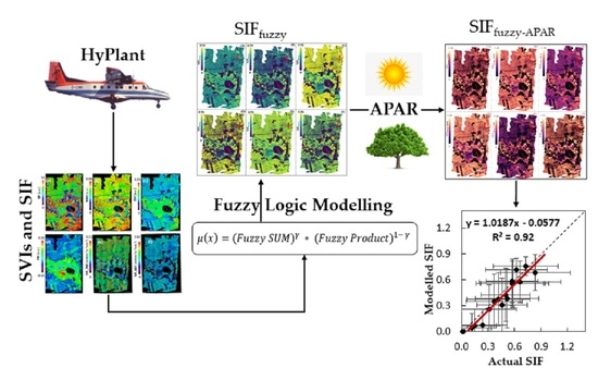
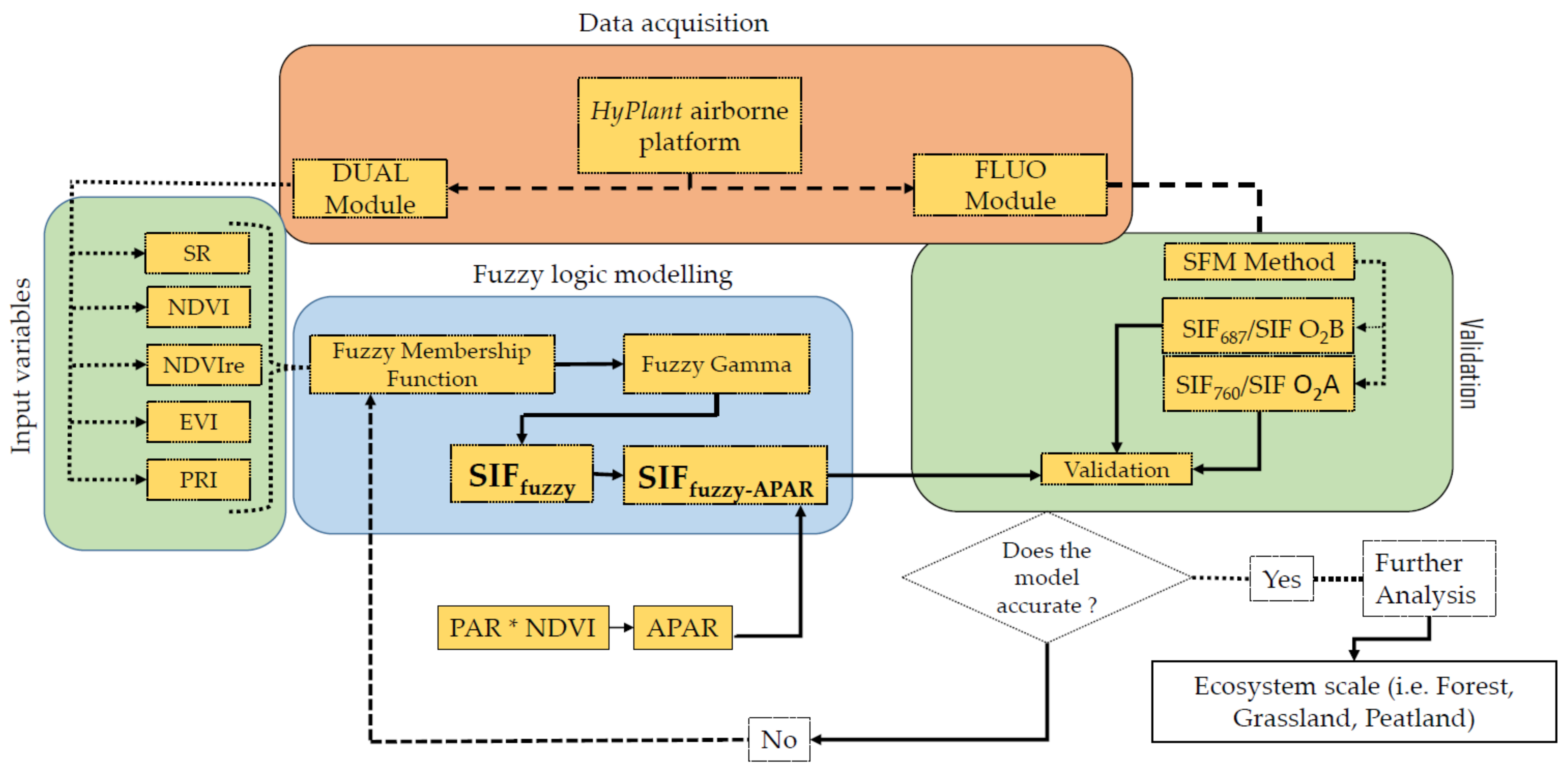
2.5. Fuzzy Logic Modelling of SIF Proxy from Reflectance-Based Vegetation Indices

The detailed theoretical description of fuzzy logic and respective algorithms have been extensively discussed by Zadeh [76]. In simple words, fuzzy logic simulates the way that people make inferences and decisions based on observations. The fuzzy logic approach allowed us to develop more flexible combinations of weighted maps and could be readily implemented using spatial modelling language. The implementation of the fuzzy logic technique based on simple SVIs using airborne acquired imaging spectroscopic data to approximate the SIF signal is a very new concept and is applied for the first time. A detailed summary of the fuzzy logic modelling approach is provided in the Supplementary Material (SM1).

The SVIs obtained from HyPlant representing different vegetation traits have a close relation to different components of SIF, as showed by Bandopadhyay et al. [1]. We have combined these SVIs and processed them through fuzzy logic modelling to develop a proxy of potential SIF and compared the modelled SIF with the actual SIF retrievals.

First, the fuzzy membership maps were retrieved from SVIs (SR, NDVI, EVI, NDVIre, PRI). Second, these membership maps were combined to obtain the final model output. In order to test whether the inclusion of APAR increases the accuracy of the model, the model outputs (SIF_fuzzy) were multiplied by APAR. Further, the final modelled outputs without (termed as SIF_fuzzy) and with the injection of APAR (termed as SIF_fuzzy-APAR) were compared and validated with the actual SIF at 687 and 760 nm maps based on validated airborne SIF data. The associated standard error (SE) and uncertainties (expressed by the root mean square error, RMSE) were also computed. The detailed methodology of the modelling approach is presented in Figure 3.

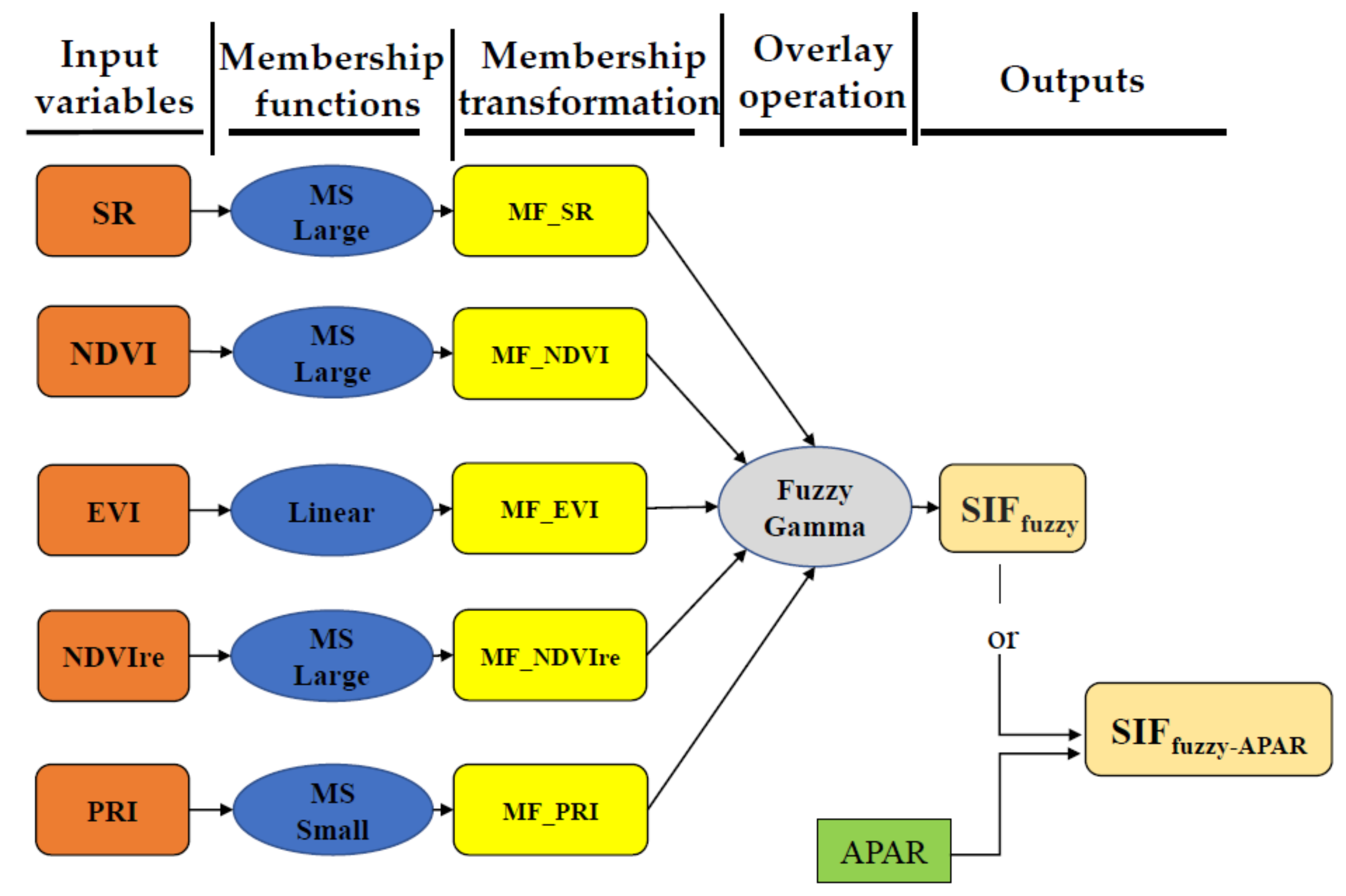
2.5.1. Fuzzy Membership Transformation

Bandopadhyay et al. [1] showed the relationship between HyPlant DUAL module derived SVIs and HyPlant FLUO module derived SIF, where SR, NDVI, EVI showed a positive agreement with increasing SIF values, while for PRI it was reversed. In agreement with these observations, the membership transformation functions for individual SVIs were selected, aiming towards the perspective to simulate a fuzzy approximation of SIF. We applied fuzzy mean-standard deviation (MS) Large function to SR, NDVI, and NDVIre, whereas fuzzy Linear and fuzzy MS Small functions were applied for EVI and PRI respectively to obtain the membership of the SVIs as input variables for the model. The fuzzy MS Large transformation function is used when the larger input values need to receive higher membership (1) and lower input values should receive lower membership (0). This transformation function is quite similar to the Fuzzy Large function, except the explanation of the function is based on a specified mean and standard deviation. Fuzzy MS Large transformation function is highly applicable and useful if the very large values are more likely to be a member of the set. In the HyPlant derived SR, NDVI, and NDVIre, the highest values were 56, 0.96, and 0.55, respectively, and they received the higher memberships, whereas, the lowest values for all indices were 0 and they received the lowest memberships (according to the HyPlant derived SR, NDVI, NDVIre scale, see Bandopadhyay et al. [1]). Similarly, the fuzzy Linear transformation function draws a linear function between the user-specified minimum and maximum values. Anything towards the defined minimum value was assigned 0 as a low membership, whereas anything towards the defined maximum value was assigned 1 as a high membership. In our model, EVI minimum value was set as 0 whereas the maximum value was set as 2.25 (according to the HyPlant derived EVI scale, see Bandopadhyay et al. [1]). The fuzzy MS Small was an opposite transformation of the fuzzy MS Large function. The fuzzy MS Small transformation function was used when the lower input values need to receive higher membership (1) and higher input values should receive lower membership (0). For PRI, we have used the fuzzy MS Small transformation function due to its negative correlation to SIF, where the lowest value of –0.43 received the highest membership and the highest value of 0.30 received the lowest membership (according to the HyPlant derived PRI scale, see Bandopadhyay et al. [1]). The justification for considering the membership transformation functions for individual SVIs aiming towards the development of SIF proxy is provided in

Table 2. The mathematical equations of membership functions and justifications for considering a membership transformation function for individual HyPlant derived SVIs.

HyPlant SVIs	Membership Functions	Equations	Justifications	References
SR	Fuzzy MS Large	$\mathsf{\mu }\left(\mathrm{x}\right)=1-\frac{\mathrm{bs}}{\mathrm{x}-\mathrm{am}+\mathrm{bs}}\mathrm{if}$ $\mathrm{x}>\mathrm{am}\mathrm{otherwise}\mathsf{\mu }\left(\mathrm{x}\right)=0$	Positive strong correlation with SIF	[1]
NDVI			Positive strong correlation with SIF	[1]
NDVIre			Positive strong correlation with SIF	(Supplementary Materials Figure S1)
EVI	Fuzzy Linear	$\mathsf{\mu }\left(\mathrm{x}\right)=\left\{\frac{\mathrm{x}-\min }{\max -\min }\right\}$	Positive poor correlation with SIF	[1]
PRI	Fuzzy MS Small	x > am otherwise μ(x) = 1 $\mathsf{\mu }\left(\mathrm{x}\right)=\frac{\mathrm{bs}}{\mathrm{x}-\mathrm{am}+\mathrm{bs}}\mathrm{if}$ $\mathrm{x}>\mathrm{am}\mathrm{otherwise}\mathsf{\mu }\left(\mathrm{x}\right)=1$	Negative correlation with SIF	[1]

.

2.5.2. Fuzzy Overlay Operation

The Fuzzy overlay operation combined the evidence that includes membership maps processed in the previous step. The justified association of different combinations in terms of memberships was highly required for the best output from fuzzy logic modelling ([77]; https://desktop.arcgis.com/en/arcmap/10.3/tools/spatial-analyst-toolbox/applying-fuzzy-logic-to-overlay-rasters.htm, accessed on 15 September 2020). There are five different types of fuzzy overlay operations that allow for such simulation: (1) Fuzzy AND, (2) Fuzzy OR, (3) Fuzzy SUM, (4) Fuzzy Product, (5) Fuzzy Gamma. The detailed information of these overlay functions has been discussed by Vakhshoori and Zare [78]. In our study, we have applied the Fuzzy Gamma function to obtain the final modelled output from the equation:

$$\mathsf{\mu }\left(\mathrm{x}\right)={\left(Fuzzy SUM\right)}^{\gamma }\ast {\left(Fuzzy Product\right)}^{1-\gamma } ,$$

where, $\mathsf{\mu }\left(\mathrm{x}\right)$ denotes the Fuzzy Gamma, and $\gamma$ is the power of gamma ranging between 0 and 1 that permits to control the decreasing or increasing tendency. The Fuzzy Gamma value of 1 produces an output equal to ‘Fuzzy Sum’ and the gamma value of 0 provides an output equal to ‘Fuzzy Product’. The Fuzzy Gamma is a kind of a balanced algebraic product of Fuzzy Product and Fuzzy Sum, which are both raised to the power of Gamma. The prime efficiency of Fuzzy Gamma is that it compromises the increasing effect of Fuzzy Sum and the decreasing effect of Fuzzy Product that makes it different from the other fuzzy overlay techniques. Moreover, the Fuzzy Gamma provides more flexibility than the additive weighted overlay and Fuzzy Sum or Fuzzy Product approaches that control the over-or under-estimation of the modelled outputs, which is a key focus in any physical modelling-based estimations [79].

Finally, the Fuzzy Gamma operation has been conducted through the combining of membership maps of the SR, NDVI, EVI, NDVIre, and PRI (i.e., MF_SR; MF_NDVI; MF_EVI; MF_NDVIre; MF_PRI) to get the final output of the simulation, showed in the overall schema (Figure 4). Parallelly, another modelled output has been produced with the injection of APAR into the modelled data.

We named the final Fuzzy Gamma modelled output as SIF_fuzzy and the final APAR-Fuzzy Gamma modelled outputs as SIF_fuzzy-APAR. The validation and agreement of both modelled outputs in reference to actual SIF signals at 760 nm and 687 nm have been conducted at the vegetation group scale along with associated error and uncertainty estimations.

2.5.3. Experiment on Different Fuzzy Combinations

In order to understand which combination of vegetation traits (in terms of SVIs) would be the most suitable to derive a proxy for actual SIF estimations and are most sensitive to predict the SIF at 760 nm and 687 nm, we run the experiment by increasing the number of inputs SVIs. We have tested the Fuzzy Gamma simulation incorporating different membership combinations to identify the best combination that can approximate the actual SIF retrievals with the highest accuracy. Different combinations of vegetation parameters such as greenness content, biomass, xanthophyll cycle, red-edge position assembled in six different ways are provided in

Table 3. The fuzzy logic model combinations with objectives and equations.

Combinations	Objectives	Equations	Code
Combination 1	approximate SIF based on greenness and biomass related SVIs (without/with the inclusion of APAR)	${\mathrm{SIF}}_{\mathrm{fuzzy}}=f\left(\mathrm{NDVI}+\mathrm{EVI}\right)$ ${\mathrm{SIF}}_{\mathrm{fuzzy}-\mathrm{APAR}}=f\left(\mathrm{NDVI}+\mathrm{EVI}\right)\ast \mathrm{APAR}$	C1
Combination 2		${\mathrm{SIF}}_{\mathrm{fuzzy}}=f\left(\mathrm{SR}+\mathrm{EVI}\right)$ ${\mathrm{SIF}}_{\mathrm{fuzzy}-\mathrm{APAR}}=f\left(\mathrm{SR}+\mathrm{EVI}\right)\ast \mathrm{APAR}$	C2
Combination 3	approximate SIF based on greenness and xanthophyll cycle-related SVIs (without/with the inclusion of APAR)	${\mathrm{SIF}}_{\mathrm{fuzzy}}=f\left(\mathrm{NDVI}+\mathrm{PRI}\right)$ ${\mathrm{SIF}}_{\mathrm{fuzzy}-\mathrm{APAR}}=f\left(\mathrm{NDVI}+\mathrm{PRI}\right)\ast \mathrm{APAR}$	C3
Combination 4		${\mathrm{SIF}}_{\mathrm{fuzzy}}=f\left(\mathrm{SR}+\mathrm{PRI}\right)$ ${\mathrm{SIF}}_{\mathrm{fuzzy}-\mathrm{APAR}}=f\left(\mathrm{SR}+\mathrm{PRI}\right)\ast \mathrm{APAR}$	C4
Combination 5	approximate SIF based on greenness, biomass, and xanthophyll cycle-related SVIs (without/with the inclusion of APAR)	${\mathrm{SIF}}_{\mathrm{fuzzy}}=f\left(\mathrm{NDVI}+\mathrm{EVI}+\mathrm{PRI}\right)$ ${\mathrm{SIF}}_{\mathrm{fuzzy}-\mathrm{APAR}}=f\left(\mathrm{NDVI}+\mathrm{EVI}+\mathrm{PRI}\right)\ast \mathrm{APAR}$	C5
Combination 6	approximate SIF based on greenness, biomass, xanthophyll cycle, and red-edge position related SVIs (without/with the inclusion of APAR)	${\mathrm{SIF}}_{\mathrm{fuzzy}}=f\left(\mathrm{SR}+\mathrm{NDVI}+\mathrm{EVI}+\mathrm{NDVIre}+\mathrm{PRI}\right)$ ${\mathrm{SIF}}_{\mathrm{fuzzy}-\mathrm{APAR}}=f\left(\mathrm{SR}+\mathrm{NDVI}+\mathrm{EVI}+\mathrm{NDVIre}+\mathrm{PRI}\right)\ast \mathrm{APAR}$	C6

f stands for function.

and they are applied to calculate SIF_fuzzy and SIF_fuzzy-APAR.

2.6. Validation of the Model, Error and Uncertainty Estimation

Statistical operations have been conducted from the fuzzy logic modelled outputs (from all six combinations) as well as from the actual SIF maps at 687 nm and 760 nm based on the 19 ROIs over different vegetation groups of forest, grassland and peatland ecosystems. The linear correlation was used to test the agreement (R²) and statistical significance (p-value) of the relationships between modelled and actual data. The analysed relationships were considered to be significant if the p-value obtained from the test was lower than 0.05 (with 95% confidence interval). In order to estimate the error and associated uncertainty between modelled and actual data, standard error (SE) and root mean square error (RMSE) have been estimated accordingly.

$$\mathrm{SE}=\frac{\mathsf{\sigma }}{\sqrt{\mathrm{n}}}\mathrm{SE}=\frac{\mathrm{If}}{\sqrt{\mathrm{n}}}$$

(1)

where, SE = standard error of the sample; $\mathsf{\sigma }\mathrm{If}$ = sample standard deviation; n = number of samples.

$$\mathrm{RMSE}=\sqrt{\frac{\sum _{\mathrm{i}=1}^{\mathrm{N}}{({\mathrm{y}}_{\mathrm{i}}-{\mathrm{y}}_{\mathrm{i}\prime })}^2}{\mathrm{N}}}$$

(2)

where, N is the number of samples, and y_i and y_i′ are the observed and predicted values, respectively.

3. Results

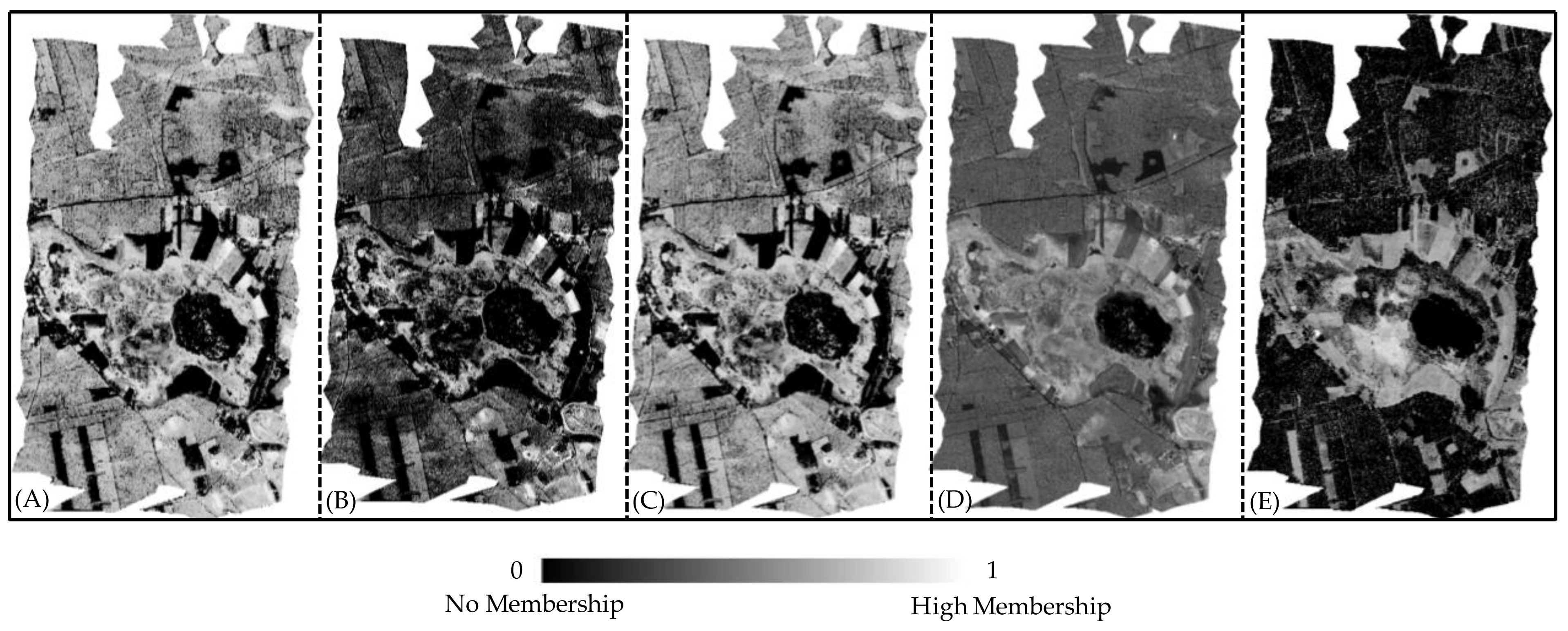
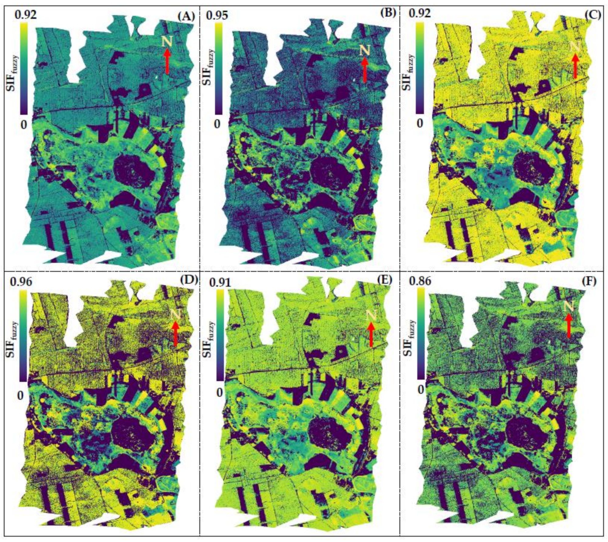
3.1. Outcome of the Membership Maps

The individual SVI maps obtained from the HyPlant DUAL module were successfully transformed to fuzzy membership maps using fuzzy membership transformation functions from Table 2. The membership transformed SVIs maps (i.e., MF_NDVI; MF_SR; MF_EVI; MF_NDVIre; MF_PRI) are presented in Figure 5. The transformed membership maps of MF_NDVI (Figure 5A), MF_SR (Figure 5B), and MF_NDVIre (Figure 5C) showed large diversity with forests and grasslands allocated with high membership, and deforested lands and mowed meadows associated with low membership. The MF_EVI map (Figure 5D) is characterized by a nearly uniform nature of membership distribution; however, it has been noticed that grasslands with dense canopies obtained the highest membership, while deforested areas inside the forests obtained no, or low membership in comparison to other ecosystems. The MF_PRI (Figure 5E) showed the opposite scenario where forest and grassland received low or no membership while the Sphagnum-dominated groups of vegetation inside the peatland obtained the highest membership. Overall fuzzy membership transformed maps showed diversity in the membership allocation based on the vegetation characteristics, structural and functional compositions.

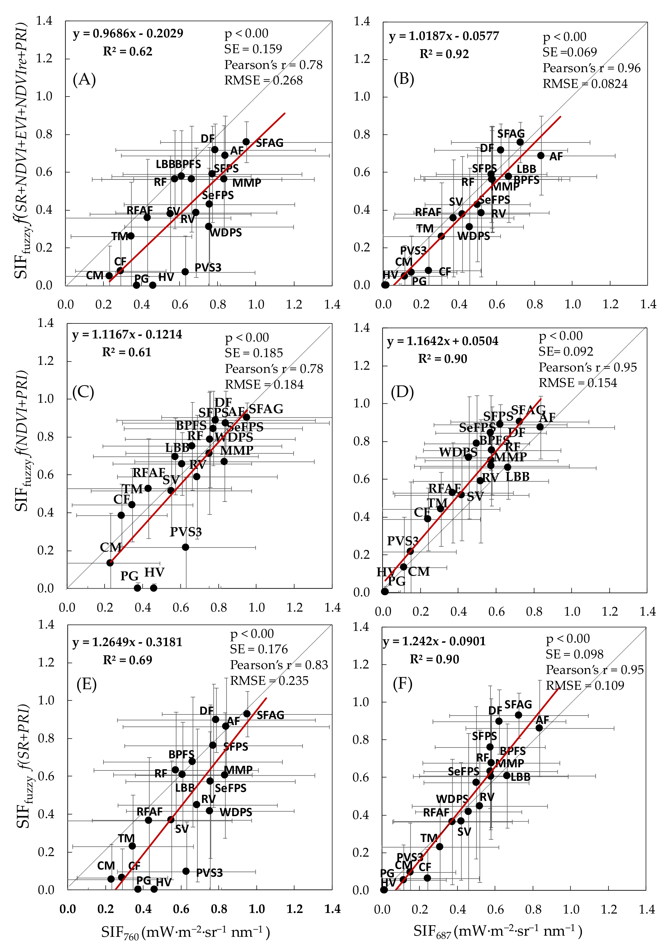
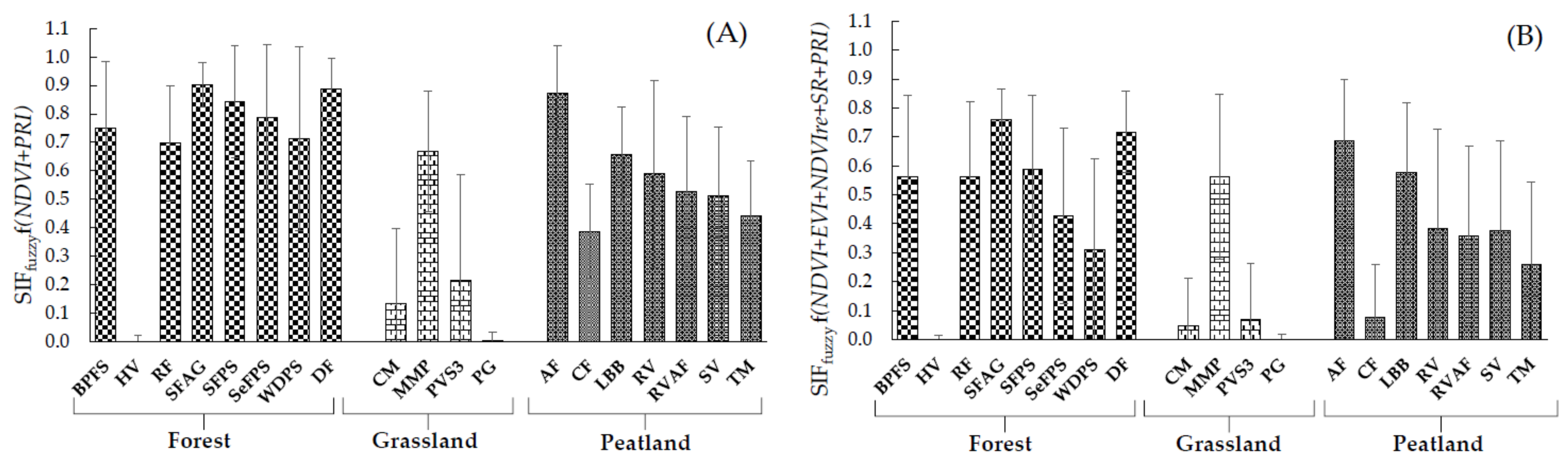
3.2. Performance of SIF_fuzzy

The SIF_fuzzy simulation based on the integration of membership SVIs and fuzzy modelling under six different combinations (C1–C6) showed a wide diversity of signals over the experimental landscape (Figure 6). The C6 SIF_fuzzy map (Figure 6F) that incorporates all the MF_SVIs shows a good consistency of signals over pine forests and meadows. The modelled signal over the peatland region is quite complex, whereas non-vegetated zones like forest clearings and post-agricultural lands are characterized with very low signals. The C6 SIF_fuzzy map ranges between 0 and 0.86. Characterized with the same consistency of signals C5 SIF_fuzzy map (Figure 6E) ranges between 0 and 0.91, whereas the C1 SIF_fuzzy (Figure 6A) and C3 SIF_fuzzy (Figure 6C) maps range between 0 and 0.92 in both scenarios. The simulated signal for C2 SIF_fuzzy (Figure 6B) map that incorporates MF_SR and MF_EVI ranges between 0 and 0.95 and C4 SIF_fuzzy (Figure 6D) map that incorporates MF_SR and MF_PRI ranges between 0 and 0.96. The distribution of modelled signals for C2 SIF_fuzzy and C4 SIF_fuzzy were very similar to previous combinations where pine forests and meadows were characterized with high signals and non-vegetated zones were characterized with low signals. The complexity of signals has been observed within peatland for all six combinations due to the wide heterogeneity of the vegetation groups. We have also observed clear differences in the absolute values of all the modelled maps (C1–C6) where C1 and C2 with the exclusion of PRI and inclusion of EVI showed lower pixel values, clearly visible mainly for forests. Whereas, intensities and contrasts are much higher for C3, C4, and C5 models with the inclusion of PRI, indicating the highest pixel values for forest ecosystems.

We found a good agreement between modelled SIF_fuzzy and actual SIF bands at SIF₇₆₀ and SIF₆₈₇ for all six combinations. However, the degree of agreement differs for different combinations (

Table 4. Summary of the statistics (R²—coefficient of determination, p-value, SE—standard error, R—correlation coefficient and RMSE—root mean square error) of linear regressions between SIF_fuzzy vs. SIF₇₆₀ and SIF_fuzzy vs. SIF₆₈₇. The statistical operational outputs were derived based on 19 ROIs representing vegetation groups of the forest, grassland and peatland.

Combinations	SIFfuzzy Functions	R2	p-Value	SE	Pearson’s r	RMSE mW·m−2·sr−1 nm−1
SIFfuzzy vs. SIF760
C1	SIFfuzzy (NDVI+EVI)	0.38	<0.05	0.172	0.61	0.259
C2	SIFfuzzy (SR+EVI)	0.55	<0.001	0.167	0.74	0.300
C3	SIFfuzzy (NDVI+PRI)	0.61	<0.001	0.185	0.78	0.184
C4	SIFfuzzy (SR+PRI)	0.69	<0.001	0.176	0.83	0.235
C5	SIFfuzzy (NDVI+EVI+PRI)	0.51	<0.01	0.195	0.71	0.193
C6	SIFfuzzy (NDVI+EVI+NDVIre+SR+PRI)	0.62	<0.001	0.159	0.78	0.268
SIFfuzzy vs. SIF687
C1	SIFfuzzy (NDVI+EVI)	0.85	<0.001	0.083	0.92	0.090
C2	SIFfuzzy (SR+EVI)	0.89	<0.001	0.083	0.94	0.114
C3	SIFfuzzy (NDVI+PRI)	0.90	<0.001	0.092	0.95	0.154
C4	SIFfuzzy (SR+PRI)	0.90	<0.001	0.098	0.95	0.109
C5	SIFfuzzy (NDVI+EVI+PRI)	0.90	<0.001	0.086	0.95	0.143
C6	SIFfuzzy (NDVI+EVI+NDVIre+SR+PRI)	0.92	<0.001	0.069	0.96	0.082

, Figure 7). The SIF_fuzzy model under C4 (f(SR+PRI)) was identified as the best performing proxy combination for SIF₇₆₀ recorded with the highest R² of 0.69 and RMSE of 0.235 mW·m⁻²·sr⁻¹ nm⁻¹ (Table 4). The second-best performing proxy combination for SIF₇₆₀ was the SIF_fuzzy model under C6 (f(NDVI+EVI+NDVIre+SR+PRI)) recorded with the R² of 0.62 and RMSE of 0.268 mW·m⁻²·sr⁻¹ nm⁻¹. However, the simulated values of SIF_fuzzy for these models (Figure 7A,E), as well as for C1 and C2 (Figure S2), were underestimated in reference to actual SIF signals at 760 nm. SIF_fuzzy models for SIF₇₆₀ under C3 (f(NDVI+PRI)) and C5 (f(NDVI+EVI+PRI)) were recorded with the lowest RMSE of 0.184 and 0.193 mW·m⁻²·sr⁻¹ nm⁻¹, respectively.

Similarly, the SIF_fuzzy model under C6 (f(NDVI+EVI+NDVIre+SR+PRI)) has been identified as the best performing proxy combination for SIF₆₈₇ recorded with the highest R² of 0.92 and RMSE of 0.082 mW·m⁻²·sr⁻¹ nm⁻¹ (Table 4). The second-best performing proxy combination for SIF₆₈₇ recorded with the RMSE of 0.09 mW·m⁻²·sr⁻¹ nm⁻¹ was the SIF_fuzzy model under C1 (f(NDVI+EVI)). The SIF_fuzzy simulations under C3 (f(NDVI+PRI)), C4 (f(SR+PRI)) and C5 (f(NDVI+EVI+PRI)) models, although correlated very well with the measured SIF₆₈₇ (R² = 0.90), were recorded with a higher RMSE of 0.154, 0.109, 0.143 mW·m⁻²·sr⁻¹ nm⁻¹, respectively, and tend to overestimate the simulated SIF_fuzzy (Figure 7D,F and Figure S2). The model outputs of C2 (f(SR+EVI)) recorded with RMSE of 0.114 mW·m⁻²·sr⁻¹ nm⁻¹ tend to slightly underestimate the simulated SIF_fuzzy (Figure S2), but the rate of underestimation and difference from the best C6 model outputs is very low.

The best performing proxy combinations under models C3 and C6 have a good agreement with the actual SIF₇₆₀ (Figure 7C) and SIF₆₈₇ (Figure 7B), respectively. The agreements between modelled and actual data demonstrated that SIF_fuzzy worked very well and can approximate the actual SIF signals at 760 nm and 687 nm with an error smaller than 10% for ecosystems where the maximum SIF values are close to 1.0 mW·m⁻²·sr⁻¹ nm⁻¹. The diversity of SIF_fuzzy signals from different vegetation groups have been observed from these agreements too (Figure 8 and Figure S3) and they correspond well to the diversity of SIF values shown in Bandopadhyay et al. [1].

We have observed from Figure 7 and Figure 8 that within forest ecosystem DF, SPAG, SFPS, BPFS vegetation groups gained the highest signals from the modelled SIF_fuzzy under C3 and C6 combinations. The WDPS and RF gained moderate signals from the modelled data, whereas, due to no vegetation cover, HV is characterized with poor modelled signals. MMP was the only vegetation group within the grassland ecosystem that received the highest signals, whereas CM, PG, PVS3 received low signals from the modelled SIF_fuzzy data. The signals obtained from the peatland ecosystem were quite complex. The AF and LBB were the two vegetation groups within peatland that received the highest modelled SIF_fuzzy signals and RV, RVAF, SV, TM received moderate signals. The weakest modelled signal under both combinations received CF within the peatland vegetation group. The estimation of modelled SIF_fuzzy signals for other combinations from 19 vegetation groups is provided in Supplementary Figure S3.

3.3. Performance of SIF_Fuzzy-APAR

The SIF_fuzzy-APAR modelled data developed through the injection of APAR into the SIF_fuzzy under six different combinations (C1–C6) showed a very prominent wide diversity of signals over different vegetation groups as well as over different ecosystems. The detailed outcome of the SIF_fuzzy-APAR including the SIF_fuzzy-APAR maps and the agreement between modelled and actual data at both SIF bands have been provided in the Supplementary Materials SM2.

4. Discussion

Bandopadhyay et al. [1] showed the agreement between SIF₇₆₀ and SIF₆₈₇ with individual SVIs at vegetation group scale under different ecosystems using HyPlant data. Although there were quite good agreements between some of the SVIs and SIF, the relationships were not optimum. However, an integrated fuzzy logic modelling technique incorporating different airborne SVIs allowed us for the first time to develop a reliable proxy of SIF₇₆₀ and SIF₆₈₇ evident by strong agreement, statistical significances, and low uncertainties. The SIF is influenced by different factors such as light absorption and interception, canopy structure influencing the fluorescence escape, and light use efficiency partially related to NPQ [80,81]. NDVI, SR, EVI, and NDVIre are greenness indices that are related to light absorption and interception, whereas EVI and NDVIre better present the canopy structure, thus they can be more related to fesc, while PRI is the component related to the light use efficiency and NPQ processes [13,17]. Considering the above, we combined different SVIs to approximate the potential SIF signals by including indices reflecting different factors controlling SIF emission. We proceeded by combining the greenness indices such as NDVI and EVI (C1), as well as SR and EVI (C2) which covered SIF influencing factors related to photon interception and canopy structure, whereas addition of PRI to greenness indices NDVI and SR (C3, C4) covered also the light use efficiency and NPQ processes influencing the SIF. We also combined NDVI, EVI, and PRI (C5) and NDVI, SR, EVI, NDVIre, and PRI (C6) to cover all three SIF influencing factors to some extent. Through C1 and C2 combinations, the modelled SIF_fuzzy explained between 38% and 55% of the variability in SIF₇₆₀ and from 85% to 89% for SIF₆₈₇. By the C3 and C4 combinations, we approximated SIF_fuzzy which explained from 61% to 69% and 90% of the variability in SIF₇₆₀ and SIF₆₈₇, respectively. Through C5 and C6 combinations, our modelled SIF_fuzzy explained from 51% to 62% and from 90% to 92% of SIF₇₆₀ and SIF₆₈₇ variability, respectively. The SIF_fuzzy showed the lowest RMSE with a high value of R² in the C3 f(NDVI + PRI) model for SIF₇₆₀, and C6 f(NDVI+EVI+NDVIre+SR+PRI) model for SIF₆₈₇. SIF₇₆₀ is known to be influenced by canopy chlorophyll concentration and is having less influence on canopy structure in comparison to SIF₆₈₇ where fesc plays a key role in SIF emission [65,82]. This is probably why the addition of EVI did not improve model accuracy for SIF₇₆₀. Whereas, the best result with the combination of five SVIs for SIF₆₈₇ showed the sensitivity and complexity of SIF₆₈₇. It showed that the combination of different SVIs reflecting variable factors controlling SIF emission like photon interception, fesc, light-use efficiency, and NPQ process improved the approximation of SIF in our models. The remaining residuals (from 62% at C1 to 38% at C6 for SIF₇₆₀ and from 15% at C1 to 8% at C6 for SIF_687, see Table 3) decreased with the increasing number of SVIs considered in the study. This may indicate that through the inclusion of different SVIs we were able to reflect the functional contribution of different factors controlling SIF at the top-of-canopy level. At the same time, relatively large residuals indicated that 100% prediction by this method is not possible as the fuzzy logic modelling process cannot mimic the functional contribution of all the different physiological processes influencing SIF emission (such as e.g., fluorescence quantum efficiency). This may be due to the different proportions and accuracy of SIF controlling factors covered through SVIs. We would assume that the contribution of such residuals may increase under the influence of stress factors over different vegetation types and hence the applicability of such a fuzzy logic modelling approach in SIF approximation under this condition might be limited. However, it has been evident that the ensemble of SVIs can approximate the SIF signals in more efficient and promising ways rather than individual SVIs representing different SIF emission factors and different vegetation traits.

The relationship of SIF with APAR is also evident and shown by several researchers (e.g., Zhang et al., [83], Wieneke et al. [66], Wohlfart et al. [84]); hence, we added APAR into our combined fuzzy logic model. The product of this simulation SIF_fuzzy-APAR was compared with SIF₆₈₇ and SIF₇₆₀ and it was observed to be best fitted to the outputs of the C1 model including NDVI and EVI (Table S5 in SM2 Supplementary Material). The inclusion of APAR slightly overestimated the SIF but also improved the R² in the case of SIF_760. SIF and APAR both are energy flux, therefore an improvement of SIF_fuzzy to SIF₇₆₀ signal by the injecting of APAR was expected and supported by, e.g., Yang et al. [13], who expressed SIF as a product of APAR and effective light use efficiency that directly connects to the fluorescence yield of the canopy. Moreover, this study includes a particular time image of the APAR and injects it with SIF_fuzzy to boost the model. We assume that after some training the use of different APAR images composed with different irradiance values can be considered as a prime variable to scale the SIF_fuzzy at a different time of the day. The overestimation of SIF_fuzzy-APAR has been particularly observed for dense forest canopies (i.e., DF, SFPS, SFAG, SeFPS) in reference to SIF₇₆₀ which was in agreement with Jung et al. [85] and Forrester et al. [86]. For SIF₆₈₇, the modelled overestimations of SIF_fuzzy-APAR have been observed in overall vegetation groups. Despite this, the overestimation of SIF was minor and our model outputs showed that an integrated fuzzy logic model can replicate the actual SIF values at both oxygen absorption bands and the derived model output values were also reasonable in reference to actual ranges. The existing studies that simulate SIF signals from reflectance spectra mostly focused on the far-red SIF range (ranging from around 740 nm to 760 nm) [35,50]. While, our model is proved to approximate SIF signals not only in the far-red region but also in a narrower SIF₆₈₇.

It has been well shown that SIF signals have a direct connection with the plant photosynthetic activity, reported by several studies [2,43]. However, photosynthetic activity has been regulated and controlled by several other aspects of plants such as vegetation type, phenology, biomass, state of health, coverage, interactions with the environment, etc. [51,87]. However, the individual SVIs can only be partially related to SIF. The integrated fuzzy logic modelling technique with the combination of several SVIs and APAR tends to minimize the differences between the predicted and actual SIF as reported in our study and can successfully approximate the SIF signals at both oxygen absorption bands. Even if the SIF signals were slightly overestimated, we have observed that the SIF_fuzzy-APAR produced a higher correlation (observed by improved R² values) with actual SIF signals in comparison to SIF_fuzzy under all C1–C6 combinations. The SIF_fuzzy-APAR or SIF_fuzzy not only have an agreement with the actual SIF signals at 760 nm and 687 nm but also well represent the diversity of SIF signals within different homogenous and heterogenous vegetation groups.

This study is the first attempt that approximates the SIF signal developed at an ecologically relevant scale due to the implementation of high-resolution airborne images (1 m), whereas most of the similar studies were conceptually implemented only at satellite levels with coarse spatial resolution. Hence, it is evident that trait-sensitive SVIs were well capable to act as a proxy for SIF if they were modelled properly, such as through integrated fuzzy logic modelling techniques, in agreement with Zhang et al. [50,83] and Guo et al. [35]. Figure 7 and Figure S10 (SM2 Supplementary Material) showed a good correlation between HyPlant-derived SIF values and modelled SIF_fuzzy and SIF_fuzzy-APAR for different vegetation groups. Thus, it means that the assimilation of plant physiological and biophysical information through fuzzy logic modelling was capable not only to approximate SIF but can also provide vital information on vegetation diversity [88]. The vegetation canopy structure influences the absorption, scattering, transmission of plants that directly affects the overall emission of fluorescence photons at the top of the canopy [89,90]. This is why, due to lower photosynthetic activities and no green cover, the deforested area, mowed meadows, and post-agricultural lands have been characterized with no values in our modelled data. Inside the peatland, alder forest and low birch bush were characterized with higher values of SIF_fuzzy and SIF_fuzzy-APAR, whereas transition mires were characterized with low values of SIF_fuzzy.

However, in this study, the fuzzy logic model has been applied over a local scale using HyPlant data. A similar methodological approach should be implemented at global scales for different ecosystems in order to verify the validity of the proposed new method of SIF approximation.

5. Conclusions

The novel development of our research termed as SIF_fuzzy and SIF_fuzzy-APAR was the first experimental evidence for quantitative demonstration of the fuzzy logic approach showing that the combination of SIF influencing factors represented by different SVIs can approximate the potential SIF signals at both oxygen absorption bands at 760 nm and 687 nm. It also demonstrated the efficiency of the integrated fuzzy logic model towards the step-by-step approximation of SIF signals through a process-based approach. This is also the first study that considers the red fluorescence into the prediction process which is extremely new and not covered in other published works.

Our experiment was also the first that reports the ability of simple airborne reflectance-based SVIs to produce a proxy of potential SIF. Both SIF_fuzzy and SIF_fuzzy-APAR worked quite accurately to approximate the SIF signals, where SIF_fuzzy were closer to SIF₆₈₇ values, whereas SIF_fuzzy-APAR were better correlated with SIF₇₆₀ as expressed by higher R² and lower RMSE.

Hence, it has been evident and recommended that the utilization of SIF_fuzzy under models C3 and C4 for SIF₇₆₀ and C6 for SIF₆₈₇ or SIF_fuzzy-APAR under C6 for both SIF₇₆₀ and SIF₆₈₇ would be the optimum solution to develop the proxy of potential SIF signals at 760 nm and 687 nm with high accuracy. The study also showed that EVI and NDVI, which can be available from spaceborne products, can be used to approximate the SIF signals to some extent. Although this study employed one-day airborne campaign data, the outcome of this study demonstrated a promising method to develop a proxy of potential SIF, where and when SIF data are not easily available or under data constraint situations. Though the proposed method does not have a significant impact on the change of observation day, slight changes in the agreements may occur during seasonal changes and atmospheric anomalies.

As we have applied the HyPlant airborne datasets, which is the airborne demonstrator for Fluorescence Explorer (FLEX) Sentinel 3 FLORIS satellite, we believe our study will significantly contribute to the ESA FLEX mission research and existing SIF studies. We believe also that the contribution from our study and the development of SIF_fuzzy, and SIF_fuzzy-APAR models will enrich our understanding of SIF science and global carbon cycles. We have not performed the SIF_fuzzy and SIF_fuzzy-APAR on the satellite dataset, but we believe that the model will work for it (however, it still needs to be validated). Thus, the proposed model is possible to be applied through satellite-derived SVIs from Sentinel 2, Landsat, MODIS, etc. to develop a SIF proxy and can be related to SIF products retrieved from spaceborne OCO-2 or GOME-2 satellites. We proved that our modelled SIF_fuzzy and SIF_fuzzy-APAR are capable to reflect the diversity of potential plant photosynthetic activity from multiple ecosystems. Therefore, such studies may further develop our knowledge of the local, regional and global photosynthetic activity and the carbon cycle in natural ecosystems.

References

1. Bandopadhyay, S.; Rastogi, A.; Rascher, U.; Rademske, P.; Schickling, A.; Cogliati, S.; Julitta, T.; Mac Arthur, A.; Hueni, A.; Tomelleri, E.; et al. Hyplant-derived Sun-Induced Fluorescence-A new opportunity to disentangle complex vegetation signals from diverse vegetation types. Remote Sens. 2019, 11, 1691. [Google Scholar] [CrossRef] [Green Version]
2. Bandopadhyay, S.; Rastogi, A.; Juszczak, R. Review of top-of-canopy sun-induced fluorescence (Sif) studies from ground, uav, airborne to spaceborne observations. Sensors 2020, 20, 1144. [Google Scholar] [CrossRef] [PubMed] [Green Version]
3. Colombo, R.; Celesti, M.; Bianchi, R.; Campbell, P.K.E.; Cogliati, S.; Cook, B.D.; Corp, L.A.; Damm, A.; Domec, J.C.; Guanter, L.; et al. Variability of sun-induced chlorophyll fluorescence according to stand age-related processes in a managed loblolly pine forest. Glob. Chang. Biol. 2018, 24, 2980–2996. [Google Scholar] [CrossRef] [Green Version]
4. Drusch, M.; Moreno, J.; Del Bello, U.; Franco, R.; Goulas, Y.; Huth, A.; Kraft, S.; Middleton, E.M.; Miglietta, F.; Mohammed, G.; et al. The FLuorescence EXplorer Mission Concept-ESA’s Earth Explorer 8. IEEE Trans. Geosci. Remote Sens. 2017, 55, 1273–1284. [Google Scholar] [CrossRef]
5. Meroni, M.; Rossini, M.; Guanter, L.; Alonso, L.; Rascher, U.; Colombo, R.; Moreno, J. Remote sensing of solar-induced chlorophyll fluorescence: Review of methods and applications. Remote Sens. Environ. 2009, 113, 2037–2051. [Google Scholar] [CrossRef]
6. Walther, S.; Voigt, M.; Thum, T.; Gonsamo, A.; Zhang, Y.; Köhler, P.; Jung, M.; Varlagin, A.; Guanter, L. Satellite chlorophyll fluorescence measurements reveal large-scale decoupling of photosynthesis and greenness dynamics in boreal evergreen forests. Glob. Chang. Biol. 2016, 22, 2979–2996. [Google Scholar] [CrossRef] [PubMed] [Green Version]
7. Gentine, P.; Alemohammad, S.H. Reconstructed Solar-Induced Fluorescence: A Machine Learning Vegetation Product Based on MODIS Surface Reflectance to Reproduce GOME-2 Solar-Induced Fluorescence. Geophys. Res. Lett. 2018, 45, 3136–3146. [Google Scholar] [CrossRef]
8. Smith, W.K.; Biederman, J.A.; Scott, R.L.; Moore, D.J.P.; He, M.; Kimball, J.S.; Yan, D.; Hudson, A.; Barnes, M.L.; MacBean, N.; et al. Chlorophyll Fluorescence Better Captures Seasonal and Interannual Gross Primary Productivity Dynamics Across Dryland Ecosystems of Southwestern North America. Geophys. Res. Lett. 2018, 45, 748–757. [Google Scholar] [CrossRef]
9. Damm, A.; Elber, J.; Erler, A.; Gioli, B.; Hamdi, K.; Hutjes, R.; Kosvancova, M.; Meroni, M.; Miglietta, F.; Moersch, A.; et al. Remote sensing of sun-induced fluorescence to improve modeling of diurnal courses of gross primary production (GPP). Glob. Chang. Biol. 2010, 16, 171–186. [Google Scholar] [CrossRef]
10. Lu, X.; Cheng, X.; Li, X.; Tang, J. Opportunities and challenges of applications of satellite-derived sun-induced fluorescence at relatively high spatial resolution. Sci. Total Environ. 2018, 619–620, 649–653. [Google Scholar] [CrossRef]
11. Mohammed, G.H.; Colombo, R.; Middleton, E.M.; Rascher, U.; van der Tol, C.; Nedbal, L.; Goulas, Y.; Pérez-Priego, O.; Damm, A.; Meroni, M.; et al. Remote sensing of solar-induced chlorophyll fluorescence (SIF) in vegetation: 50 years of progress. Remote Sens. Environ. 2019, 231, 111177. [Google Scholar] [CrossRef]
12. Porcar-Castell, A.; Tyystjärvi, E.; Atherton, J.; Van Der Tol, C.; Flexas, J.; Pfündel, E.E.; Moreno, J.; Frankenberg, C.; Berry, J.A. Linking chlorophyll a fluorescence to photosynthesis for remote sensing applications: Mechanisms and challenges. J. Exp. Bot. 2014, 65, 4065–4095. [Google Scholar] [CrossRef]
13. Yang, K.; Ryu, Y.; Dechant, B.; Berry, J.A.; Hwang, Y.; Jiang, C.; Kang, M.; Kim, J.; Kimm, H.; Kornfeld, A.; et al. Sun-induced chlorophyll fluorescence is more strongly related to absorbed light than to photosynthesis at half-hourly resolution in a rice paddy. Remote Sens. Environ. 2018, 216, 658–673. [Google Scholar] [CrossRef]
14. Fournier, A.; Daumard, F.; Champagne, S.; Ounis, A.; Goulas, Y.; Moya, I. Effect of canopy structure on sun-induced chlorophyll fluorescence. ISPRS J. Photogramm. Remote Sens. 2012, 68, 112–120. [Google Scholar] [CrossRef]
15. Van der Tol, C.; Rossini, M.; Cogliati, S.; Verhoef, W.; Colombo, R.; Rascher, U.; Mohammed, G. A model and measurement comparison of diurnal cycles of sun-induced chlorophyll fluorescence of crops. Remote Sens. Environ. 2016, 186, 663–677. [Google Scholar] [CrossRef]
16. Zan, M.; Zhou, Y.; Ju, W.; Zhang, Y.; Zhang, L.; Liu, Y. Performance of a two-leaf light use efficiency model for mapping gross primary productivity against remotely sensed sun-induced chlorophyll fluorescence data. Sci. Total Environ. 2018, 613–614, 977–989. [Google Scholar] [CrossRef]
17. Miao, G.; Guan, K.; Yang, X.; Bernacchi, C.J.; Berry, J.A.; DeLucia, E.H.; Wu, J.; Moore, C.E.; Meacham, K.; Cai, Y.; et al. Sun-Induced Chlorophyll Fluorescence, Photosynthesis, and Light Use Efficiency of a Soybean Field from Seasonally Continuous Measurements. J. Geophys. Res. Biogeosci. 2018, 123, 610–623. [Google Scholar] [CrossRef]
18. Sakamoto, T.; Gitelson, A.A.; Wardlow, B.D.; Verma, S.B.; Suyker, A.E. Estimating daily gross primary production of maize based only on MODIS WDRVI and shortwave radiation data. Remote Sens. Environ. 2011, 115, 3091–3101. [Google Scholar] [CrossRef]
19. Juszczak, R.; Uździcka, B.; Stróżecki, M.; Sakowska, K. Improving remote estimation of winter crops gross ecosystem production by inclusion of leaf area index in a spectral model. PeerJ 2018, 2018, e5613. [Google Scholar] [CrossRef] [Green Version]
20. Wolanin, A.; Camps-Valls, G.; Gómez-Chova, L.; Mateo-García, G.; van der Tol, C.; Zhang, Y.; Guanter, L. Estimating crop primary productivity with Sentinel-2 and Landsat 8 using machine learning methods trained with radiative transfer simulations. Remote Sens. Environ. 2019, 225, 441–457. [Google Scholar] [CrossRef]
21. Sakowska, K.; Vescovo, L.; Marcolla, B.; Juszczak, R.; Olejnik, J.; Gianelle, D. Monitoring of carbon dioxide fluxes in a subalpine grassland ecosystem of the Italian Alps using a multispectral sensor. Biogeosciences 2014, 11, 4695–4712. [Google Scholar] [CrossRef]
22. Rastogi, A.; Antala, M.; Gąbka, M.; Rosadziński, S.; Stróżecki, M.; Brestic, M.; Juszczak, R. Impact of warming and reduced precipitation on morphology and chlorophyll concentration in peat mosses (Sphagnum angustifolium and S. fallax). Sci. Rep. 2020, 10, 1–9. [Google Scholar] [CrossRef] [PubMed]
23. Cole, B.; McMorrow, J.; Evans, M. Spectral monitoring of moorland plant phenology to identify a temporal window for hyperspectral remote sensing of peatland. ISPRS J. Photogramm. Remote Sens. 2014, 90, 49–58. [Google Scholar] [CrossRef]
24. Rahaman, K.R.; Hassan, Q.K.; Ahmed, M.R. Pan-sharpening of landsat-8 images and its application in calculating vegetation greenness and canopy water contents. ISPRS Int. J. Geo-Inf. 2017, 6, 168. [Google Scholar] [CrossRef] [Green Version]
25. Wong, C.Y.S.; D’Odorico, P.; Bhathena, Y.; Arain, M.A.; Ensminger, I. Carotenoid based vegetation indices for accurate monitoring of the phenology of photosynthesis at the leaf-scale in deciduous and evergreen trees. Remote Sens. Environ. 2019, 233, 111407. [Google Scholar] [CrossRef]
26. Roy, P.S.; Ravan, S.A. Biomass estimation using satellite remote sensing data—An investigation on possible approaches for natural forest. J. Biosci. 1996, 21, 535–561. [Google Scholar] [CrossRef]
27. Kumar, L.; Mutanga, O. Remote sensing of above-ground biomass. Remote Sens. 2017, 9, 935. [Google Scholar] [CrossRef] [Green Version]
28. Cohen, W.B. Response of vegetation indices to changes in three measures of leaf water stress. Photogramm. Eng. Remote Sens. 1991, 57, 195–202. [Google Scholar]
29. Nagler, P.L.; Glenn, E.P.; Kim, H.; Emmerich, W.; Scott, R.L.; Huxman, T.E.; Huete, A.R. Relationship between evapotranspiration and precipitation pulses in a semiarid rangeland estimated by moisture flux towers and MODIS vegetation indices. J. Arid Environ. 2007, 70, 443–462. [Google Scholar] [CrossRef]
30. Liu, Y.; Dang, C.; Yue, H.; Lyu, C.; Dang, X. Enhanced drought detection and monitoring using sun-induced chlorophyll fluorescence over Hulun Buir Grassland, China. Sci. Total Environ. 2021, 770, 145271. [Google Scholar] [CrossRef]
31. Gong, P.; Pu, R.; Biging, G.S.; Larrieu, M.R. Estimation of forest leaf area index using vegetation indices derived from Hyperion hyperspectral data. IEEE Trans. Geosci. Remote Sens. 2003, 41, 1355–1362. [Google Scholar] [CrossRef] [Green Version]
32. Dong, T.; Liu, J.; Shang, J.; Qian, B.; Ma, B.; Kovacs, J.M.; Walters, D.; Jiao, X.; Geng, X.; Shi, Y. Assessment of red-edge vegetation indices for crop leaf area index estimation. Remote Sens. Environ. 2019, 222, 133–143. [Google Scholar] [CrossRef]
33. Peguero-Pina, J.J.; Morales, F.; Flexas, J.; Gil-Pelegrín, E.; Moya, I. Photochemistry, remotely sensed physiological reflectance index and de-epoxidation state of the xanthophyll cycle in Quercus coccifera under intense drought. Oecologia 2008, 156, 1–11. [Google Scholar] [CrossRef] [PubMed]
34. Harris, A.; Gamon, J.A.; Pastorello, G.Z.; Wong, C.Y.S. Retrieval of the photochemical reflectance index for assessing xanthophyll cycle activity: A comparison of near-surface optical sensors. Biogeosciences 2014, 11, 6277–6292. [Google Scholar] [CrossRef] [Green Version]
35. Guo, M.; Li, J.; Huang, S.; Wen, L. Feasibility of using MODIS products to simulate sun-induced chlorophyll fluorescence (SIF) in boreal forests. Remote Sens. 2020, 12, 680. [Google Scholar] [CrossRef] [Green Version]
36. Zarate-Valdez, J.L.; Metcalf, S.; Stewart, W.; Ustin, S.L.; Lampinen, B. Potentials and limits of vegetation indices for LAI and APAR assessment. Precis. Agric. 2015, 16, 161–173. [Google Scholar]
37. Li, X.; Xiao, J.; He, B.; Altaf Arain, M.; Beringer, J.; Desai, A.R.; Emmel, C.; Hollinger, D.Y.; Krasnova, A.; Mammarella, I.; et al. Solar-induced chlorophyll fluorescence is strongly correlated with terrestrial photosynthesis for a wide variety of biomes: First global analysis based on OCO-2 and flux tower observations. Glob. Chang. Biol. 2018, 24, 3990–4008. [Google Scholar] [CrossRef] [PubMed]
38. Gamon, J.A.; Field, C.B.; Goulden, M.L.; Griffin, K.L.; Hartley, E.; Joel, G.; Peñuelas, J.; Valentini, R. Relationships between NDVI, Canopy Structure, and Photosynthesis in Three Californian Vegetation Types. Ecol. Appl. 1995, 5, 28–41. [Google Scholar] [CrossRef] [Green Version]
39. Huete, A.; Didan, K.; Miura, T.; Rodriguez, E.P.; Gao, X.; Ferreira, L.G. Overview of the radiometric and biophysical performance of the MODIS vegetation indices. Remote Sens. Environ. 2002, 83, 195–213. [Google Scholar] [CrossRef]
40. Evangelides, C.; Nobajas, A. Red-Edge Normalised Difference Vegetation Index (NDVI705) from Sentinel-2 imagery to assess post-fire regeneration. Remote Sens. Appl. Soc. Environ. 2020, 17, 100283. [Google Scholar] [CrossRef]
41. Louis, J.; Ounis, A.; Ducruet, J.M.; Evain, S.; Laurila, T.; Thum, T.; Aurela, M.; Wingsle, G.; Alonso, L.; Pedros, R.; et al. Remote sensing of sunlight-induced chlorophyll fluorescence and reflectance of Scots pine in the boreal forest during spring recovery. Remote Sens. Environ. 2005, 96, 37–48. [Google Scholar] [CrossRef] [Green Version]
42. Wang, X.; Chen, J.M.; Ju, W. Photochemical reflectance index (PRI) can be used to improve the relationship between gross primary productivity (GPP) and sun-induced chlorophyll fluorescence (SIF). Remote Sens. Environ. 2020, 246, 111888. [Google Scholar] [CrossRef]
43. Cendrero-Mateo, M.P.; Wieneke, S.; Damm, A.; Alonso, L.; Pinto, F.; Moreno, J.; Guanter, L.; Celesti, M.; Rossini, M.; Sabater, N.; et al. Sun-induced chlorophyll fluorescence III: Benchmarking retrieval methods and sensor characteristics for proximal sensing. Remote Sens. 2019, 11, 962. [Google Scholar] [CrossRef] [Green Version]
44. Rascher, U.; Alonso, L.; Burkart, A.; Cilia, C.; Cogliati, S.; Colombo, R.; Damm, A.; Drusch, M.; Guanter, L.; Hanus, J.; et al. Sun-induced fluorescence—A new probe of photosynthesis: First maps from the imaging spectrometer HyPlant. Glob. Chang. Biol. 2015, 21, 4673–4684. [Google Scholar] [CrossRef] [Green Version]
45. Rossini, M.; Nedbal, L.; Guanter, L.; Ač, A.; Alonso, L.; Burkart, A.; Cogliati, S.; Colombo, R.; Damm, A.; Drusch, M.; et al. Red and far red Sun-induced chlorophyll fluorescence as a measure of plant photosynthesis. Geophys. Res. Lett. 2015, 42, 1632–1639. [Google Scholar] [CrossRef] [Green Version]
46. Ni, Z.; Lu, Q.; Huo, H.; Zhang, H. Estimation of chlorophyll fluorescence at different scales: A review. Sensors 2019, 19, 3000. [Google Scholar] [CrossRef] [Green Version]
47. Frankenberg, C.; O’Dell, C.; Berry, J.; Guanter, L.; Joiner, J.; Köhler, P.; Pollock, R.; Taylor, T.E. Prospects for chlorophyll fluorescence remote sensing from the Orbiting Carbon Observatory-2. Remote Sens. Environ. 2014, 147, 1–12. [Google Scholar] [CrossRef] [Green Version]
48. Joiner, J.; Guanter, L.; Lindstrot, R.; Voigt, M.; Vasilkov, A.P.; Middleton, E.M.; Huemmrich, K.F.; Yoshida, Y.; Frankenberg, C. Global monitoring of terrestrial chlorophyll fluorescence from moderate-spectral-resolution near-infrared satellite measurements: Methodology, simulations, and application to GOME-2. Atmos. Meas. Tech. 2013, 6, 2803–2823. [Google Scholar] [CrossRef] [Green Version]
49. Joiner, J.; Yoshida, Y.; Vasilkov, A.P.; Schaefer, K.; Jung, M.; Guanter, L.; Zhang, Y.; Garrity, S.; Middleton, E.M.; Huemmrich, K.F.; et al. The seasonal cycle of satellite chlorophyll fluorescence observations and its relationship to vegetation phenology and ecosystem atmosphere carbon exchange. Remote Sens. Environ. 2014, 152, 375–391. [Google Scholar] [CrossRef] [Green Version]
50. Zhang, Z.; Zhang, Y.; Joiner, J.; Migliavacca, M. Angle matters: Bidirectional effects impact the slope of relationship between gross primary productivity and sun-induced chlorophyll fluorescence from Orbiting Carbon Observatory-2 across biomes. Glob. Chang. Biol. 2018, 24, 5017–5020. [Google Scholar] [CrossRef] [Green Version]
51. Zhang, Y.; Joiner, J.; Hamed Alemohammad, S.; Zhou, S.; Gentine, P. A global spatially contiguous solar-induced fluorescence (CSIF) dataset using neural networks. Biogeosciences 2018, 15, 5779–5800. [Google Scholar] [CrossRef] [Green Version]
52. Liu, L.; Liu, X.; Hu, J. Effects of spectral resolution and SNR on the vegetation solar-induced fluorescence retrieval using FLD-based methods at canopy level. Eur. J. Remote Sens. 2015, 48, 743–762. [Google Scholar] [CrossRef] [Green Version]
53. Yang, P.; van der Tol, C.; Campbell, P.K.E.; Middleton, E.M. Fluorescence Correction Vegetation Index (FCVI): A physically based reflectance index to separate physiological and non-physiological information in far-red sun-induced chlorophyll fluorescence. Remote Sens. Environ. 2020, 240, 111676. [Google Scholar] [CrossRef]
54. Badgley, G.; Field, C.B.; Berry, J.A. Canopy near-infrared reflectance and terrestrial photosynthesis. Sci. Adv. 2017, 3, 1–6. [Google Scholar] [CrossRef] [Green Version]
55. Li, X.; Xiao, J. A global, 0.05-degree product of solar-induced chlorophyll fluorescence derived from OCO-2, MODIS, and reanalysis data. Remote Sens. 2019, 11, 517. [Google Scholar] [CrossRef] [Green Version]
56. Frankenberg, C.; Fisher, J.B.; Worden, J.; Badgley, G.; Saatchi, S.S.; Lee, J.E.; Toon, G.C.; Butz, A.; Jung, M.; Kuze, A.; et al. New global observations of the terrestrial carbon cycle from GOSAT: Patterns of plant fluorescence with gross primary productivity. Geophys. Res. Lett. 2011, 38, 17. [Google Scholar] [CrossRef] [Green Version]
57. Raychaudhuri, B. Solar-induced fluorescence of terrestrial chlorophyll derived from the O2-A band of Hyperion hyperspectral images. Remote Sens. Lett. 2014, 5, 941–950. [Google Scholar] [CrossRef]
58. Irteza, S.M.; Nichol, J.E. Measurement of sun induced chlorophyll fluorescence using hyperspectral satellite imagery. In Proceedings of the International Archives of the Photogrammetry, Remote Sensing and Spatial Information Sciences—ISPRS Archives, Prague, Czech Republic, 12–19 July 2016; pp. 911–913. [Google Scholar]
59. Juszczak, R.; Augustin, J. Exchange of the greenhouse gases methane and nitrous oxide between the atmosphere and a temperate peatland in Central Europe. Wetlands 2013, 33, 895–907. [Google Scholar] [CrossRef] [Green Version]
60. Juszczak, R.; Humphreys, E.; Acosta, M.; Michalak-Galczewska, M.; Kayzer, D.; Olejnik, J. Ecosystem respiration in a heterogeneous temperate peatland and its sensitivity to peat temperature and water table depth. Plant Soil 2013, 366, 505–520. [Google Scholar] [CrossRef] [Green Version]
61. Milecka, K.; Kowalewski, G.; Fiałkiewicz-Kozieł, B.; Gałka, M.; Lamentowicz, M.; Chojnicki, B.H.; Goslar, T.; Barabach, J. Hydrological changes in the Rzecin peatland (Puszcza Notecka, Poland) induced by anthropogenic factors: Implications for mire development and carbon sequestration. Holocene 2017, 27, 651–664. [Google Scholar] [CrossRef]
62. Barabach, J. The history of Lake Rzecin and its surroundings drawn on maps as a background to palaeoecological reconstruction. Limnol. Rev. 2013, 12, 103–114. [Google Scholar] [CrossRef] [Green Version]
63. Lamentowicz, M.; Mueller, M.; Gałka, M.; Barabach, J.; Milecka, K.; Goslar, T.; Binkowski, M. Reconstructing human impact on peatland development during the past 200 years in CE Europe through biotic proxies and X-ray tomography. Quat. Int. 2015, 357, 282–294. [Google Scholar] [CrossRef]
64. Siegmann, B.; Alonso, L.; Celesti, M.; Cogliati, S.; Colombo, R.; Damm, A.; Douglas, S.; Guanter, L.; Hanuš, J.; Kataja, K.; et al. The High-Performance Airborne Imaging Spectrometer HyPlant—From Raw Images to Top-of-Canopy Reflectance and Fluorescence Products: Introduction of an Automatized Processing Chain. Remote Sens. 2019, 11, 2760. [Google Scholar] [CrossRef] [Green Version]
65. Wieneke, S.; Ahrends, H.; Damm, A.; Pinto, F.; Stadler, A.; Rossini, M.; Rascher, U. Airborne based spectroscopy of red and far-red sun-induced chlorophyll fluorescence: Implications for improved estimates of gross primary productivity. Remote Sens. Environ. 2016, 184, 654–667. [Google Scholar] [CrossRef] [Green Version]
66. Wieneke, S.; Burkart, A.; Cendrero-Mateo, M.P.; Julitta, T.; Rossini, M.; Schickling, A.; Schmidt, M.; Rascher, U. Linking photosynthesis and sun-induced fluorescence at sub-daily to seasonal scales. Remote Sens. Environ. 2018, 219, 247–258. [Google Scholar] [CrossRef]
67. Meroni, M.; Colombo, R. Leaf level detection of solar induced chlorophyll fluorescence by means of a subnanometer resolution spectroradiometer. Remote Sens. Environ. 2006, 103, 438–448. [Google Scholar] [CrossRef]
68. Meroni, M.; Barducci, A.; Cogliati, S.; Castagnoli, F.; Rossini, M.; Busetto, L.; Migliavacca, M.; Cremonese, E.; Galvagno, M.; Colombo, R.; et al. The hyperspectral irradiometer, a new instrument for long-term and unattended field spectroscopy measurements. Rev. Sci. Instrum. 2011, 82, 043106. [Google Scholar] [CrossRef]
69. Cogliati, S.; Verhoef, W.; Kraft, S.; Sabater, N.; Alonso, L.; Vicent, J.; Moreno, J.; Drusch, M.; Colombo, R. Retrieval of sun-induced fluorescence using advanced spectral fitting methods. Remote Sens. Environ. 2015, 169, 344–357. [Google Scholar] [CrossRef]
70. Cogliati, S.; Colombo, R.; Celesti, M.; Tagliabue, G.; Rascher, U.; Schickling, A.; Rademske, P.; Alonso, L.; Sabater, N.; Schuettemeyer, D.; et al. Red and far-red fluorescence emission retrieval from airborne high-resolution spectra collected by the hyplant-fluo sensor. In Proceedings of the International Geoscience and Remote Sensing Symposium (IGARSS), Valencia, Spain, 22–27 July 2018; Volume 2018, pp. 3935–3938. [Google Scholar]
71. Asrar, G.; Fuchs, M.; Kanemasu, E.T.; Hatfield, J.L. Estimating Absorbed Photosynthetic Radiation and Leaf Area Index from Spectral Reflectance in Wheat 1. Agron. J. 1984, 76, 300–306. [Google Scholar] [CrossRef]
72. Rouse, J.W.; Haas, R.H.; Schell, J.A.; Deering, D.W. Monitoring the vernal advancement and retrogradation (green wave effect) of natural vegetation. Prog. Rep. RSC 1978-1 1973, 371, 1–390. [Google Scholar]
73. Gitelson, A.; Merzlyak, M.N. Spectral Reflectance Changes Associated with Autumn Senescence of Aesculus hippocastanum L. and Acer platanoides L. Leaves. Spectral Features and Relation to Chlorophyll Estimation. J. Plant Physiol. 1994, 143, 286–292. [Google Scholar] [CrossRef]
74. Gamon, J.A.; Serrano, L.; Surfus, J.S. The photochemical reflectance index: An optical indicator of photosynthetic radiation use efficiency across species, functional types, and nutrient levels. Oecologia 1997, 112, 492–501. [Google Scholar] [CrossRef]
75. Wang, S.; Zhang, L.; Huang, C.; Qiao, N. An NDVI-based vegetation phenology is improved to be more consistent with photosynthesis dynamics through applying a light use efficiency model over boreal high-latitude forests. Remote Sens. 2017, 9, 695. [Google Scholar] [CrossRef] [Green Version]
76. Zadeh, L.A. Fuzzy sets. Inf. Control 1965, 8, 338–353. [Google Scholar] [CrossRef] [Green Version]
77. Bardhan, R.; Bandopadhyay, S.; Gupta, K. Rapid Estimation of Flood Prone Zones under Data Constraint Scenario. In Proceedings of the Hydro 2015 International viz 20th International Conference on Hydraulics, Water Resources and River Engineering, Roorkee, India, 17–19 December 2015; pp. 17–19. [Google Scholar]
78. Vakhshoori, V.; Zare, M. Landslide susceptibility mapping by comparing weight of evidence, fuzzy logic, and frequency ratio methods. Geomat. Nat. Hazards Risk 2016, 7, 1731–1752. [Google Scholar] [CrossRef]
79. Mărgărit-Mircea, N.; Harianto, R.; Alfrendo, S.; EngChoon, L.; Koh, Z.H.; Aaron, W.L.S.; Hongjun, W. Gis-Based Approach To Identify The Suitable Locations For Soil Sampling In Singapore. Geogr. Tech. 2016, 11, 39–50. [Google Scholar]
80. Yang, P.; Van Der Tol, C.; Campbell, P.K.E.; Middleton, E.M. Unraveling the physical and physiological basis for the solar-induced chlorophyll fluorescence and photosynthesis relationship using continuous leaf and canopy measurements of a corn crop. Biogeosciences 2021, 18, 441–465. [Google Scholar] [CrossRef]
81. Parazoo, N.C.; Magney, T.; Norton, A.; Raczka, B.; Bacour, C.; Maignan, F.; Baker, I.; Zhang, Y.; Qiu, B.; Shi, M.; et al. Wide discrepancies in the magnitude and direction of modeled solar-induced chlorophyll fluorescence in response to light conditions. Biogeosciences 2020, 17, 3733–3755. [Google Scholar] [CrossRef]
82. Dechant, B.; Ryu, Y.; Badgley, G.; Zeng, Y.; Berry, J.A.; Zhang, Y.; Moya, I. Canopy structure explains the relationship between photosynthesis and sun-induced chlorophyll fluorescence in crops. Remote Sens. Environ. 2020, 241, 111733. [Google Scholar] [CrossRef] [Green Version]
83. Zhang, Y.; Guanter, L.; Berry, J.A.; van der Tol, C.; Yang, X.; Tang, J.; Zhang, F. Model-based analysis of the relationship between sun-induced chlorophyll fluorescence and gross primary production for remote sensing applications. Remote Sens. Environ. 2016, 187, 145–155. [Google Scholar] [CrossRef] [Green Version]
84. Wohlfahrt, G.; Gerdel, K.; Migliavacca, M.; Rotenberg, E.; Tatarinov, F.; Müller, J.; Hammerle, A.; Julitta, T.; Spielmann, F.M.; Yakir, D. Sun-induced fluorescence and gross primary productivity during a heat wave. Sci. Rep. 2018, 8, 1–9. [Google Scholar] [CrossRef]
85. Jeong, S.J.; Schimel, D.; Frankenberg, C.; Drewry, D.T.; Fisher, J.B.; Verma, M.; Berry, J.A.; Lee, J.E.; Joiner, J. Application of satellite solar-induced chlorophyll fluorescence to understanding large-scale variations in vegetation phenology and function over northern high latitude forests. Remote Sens. Environ. 2017, 190, 178–187. [Google Scholar] [CrossRef]
86. Forrester, D.I.; Guisasola, R.; Tang, X.; Albrecht, A.T.; Dong, T.L.; Le Maire, G. Using a stand-level model to predict light absorption in stands with vertically and horizontally heterogeneous canopies. For. Ecosyst. 2014, 1, 1–19. [Google Scholar] [CrossRef]
87. Parazoo, N.C.; Bowman, K.; Fisher, J.B.; Frankenberg, C.; Jones, D.B.A.; Cescatti, A.; Pérez-Priego, Ó.; Wohlfahrt, G.; Montagnani, L. Terrestrial gross primary production inferred from satellite fluorescence and vegetation models. Glob. Chang. Biol. 2014, 20, 3103–3121. [Google Scholar] [CrossRef] [PubMed]
88. Yan, M.; Liangyun, L.; Ruonan, C.; Shanshan, D.; Xinjie, L. Generation of a Global Spatially Continuous TanSat Solar-Induced Chlorophyll Fluorescence Product by Considering the Impact of the Solar Radiation Intensity. Remote Sens. 2020, 12, 2167. [Google Scholar]
89. Zeng, Y.; Badgley, G.; Dechant, B.; Ryu, Y.; Chen, M.; Berry, J.A. A practical approach for estimating the escape ratio of near-infrared solar-induced chlorophyll fluorescence. Remote Sens. Environ. 2019, 232, 111209. [Google Scholar] [CrossRef] [Green Version]
90. Liu, X.; Guanter, L.; Liu, L.; Damm, A.; Malenovský, Z.; Rascher, U.; Peng, D.; Du, S.; Gastellu-Etchegorry, J.P. Downscaling of solar-induced chlorophyll fluorescence from canopy level to photosystem level using a random forest model. Remote Sens. Environ. 2019, 231, 110772. [Google Scholar] [CrossRef]
Figure 1. Location of the Rzecin peatland, Wielkopolska region, Poland. An RGB composite map was obtained by combining reflectance bands for the red, green, and blue bands of the HyPlant DUAL module during the Spectrometry of a Wetland and Modelling of Photosynthesis (SWAMP) campaign on 11 July 2015. (Adopted from Bandopadhyay et al. [1]).
Remotesensing 13 02545 g001
Figure 2. Location and boundaries of the 158 ROIs identified in the HyPlant RGB image and categorized into 19 unique vegetation groups. Adopted after Bandopadhyay et al. [1].
Remotesensing 13 02545 g002
Figure 3. Scheme of the research methodology and different steps of data processing from HyPlant data acquisition to model building and validation of the outputs.
Remotesensing 13 02545 g003
Figure 4. Schema of the fuzzy logic modelling system adopted in this study showing the progress from the input variable to the membership transformation in order to overlay operation to the final output.
Remotesensing 13 02545 g004
Figure 5. Membership maps of the different SVIs: (A) MF_NDVI; (B) MF_SR; (C) MF_NDVIre; (D) MF_EVI and (E) MF_PRI, derived from the fuzzy membership transformation functions. The membership maps ranging from 0 to 1 represent no membership to high membership, respectively.
Remotesensing 13 02545 g005
Figure 6. Simulated SIFfuzzy maps developed through the integration of membership maps and Fuzzy Gamma approach for C1–C6 combinations: (A) C1 SIFfuzzy; (B) C2 SIFfuzzy; (C) C3 SIFfuzzy; (D) C4 SIFfuzzy; (E) C5 SIFfuzzy; and (F) C6 SIFfuzzy. The colour stretch in the left represents the range of C1–C6 SIFfuzzy maps.
Remotesensing 13 02545 g006
Figure 7. Scatterplots of the best performing fuzzy logic model outputs (SIFfuzzy) and actual SIFs (SIF760 and SIF687) were determined based on HyPlant airborne data. (A,B) SIFfuzzy expressed by f(NDVI+EVI+NDVIre+SR+PRI) under model C6; (C,D) SIFfuzzy expressed by f(NDVI+PRI) under model C3; (E,F) SIFfuzzy expressed by f(SR+PRI) under model C4. Standard deviations are represented in error bars. The letter abbreviations correspond to the codes of vegetation groups presented in Figure 2.
Remotesensing 13 02545 g007
Figure 8. Example of bar diagrams representing the modelled values of SIFfuzzy obtained from 19 ROIs; (A) SIFfuzzy as expressed by f(NDVI+PRI) under C3; (B) SIFfuzzy as expressed by f(NDVI+EVI+NDVIre+SR+PRI) under C6. Error bars represent the standard deviations.
Remotesensing 13 02545 g008