
A Novel Change Detection Approach Based on Spectral Unmixing from Stacked Multitemporal Remote Sensing Images with a Variability of Endmembers


Abstract
:
1. Introduction
2. Relevant Background
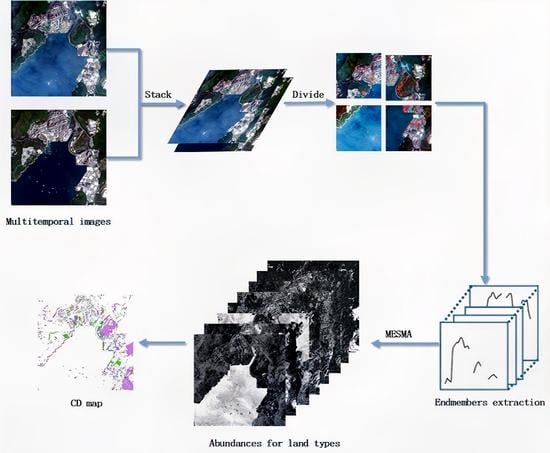
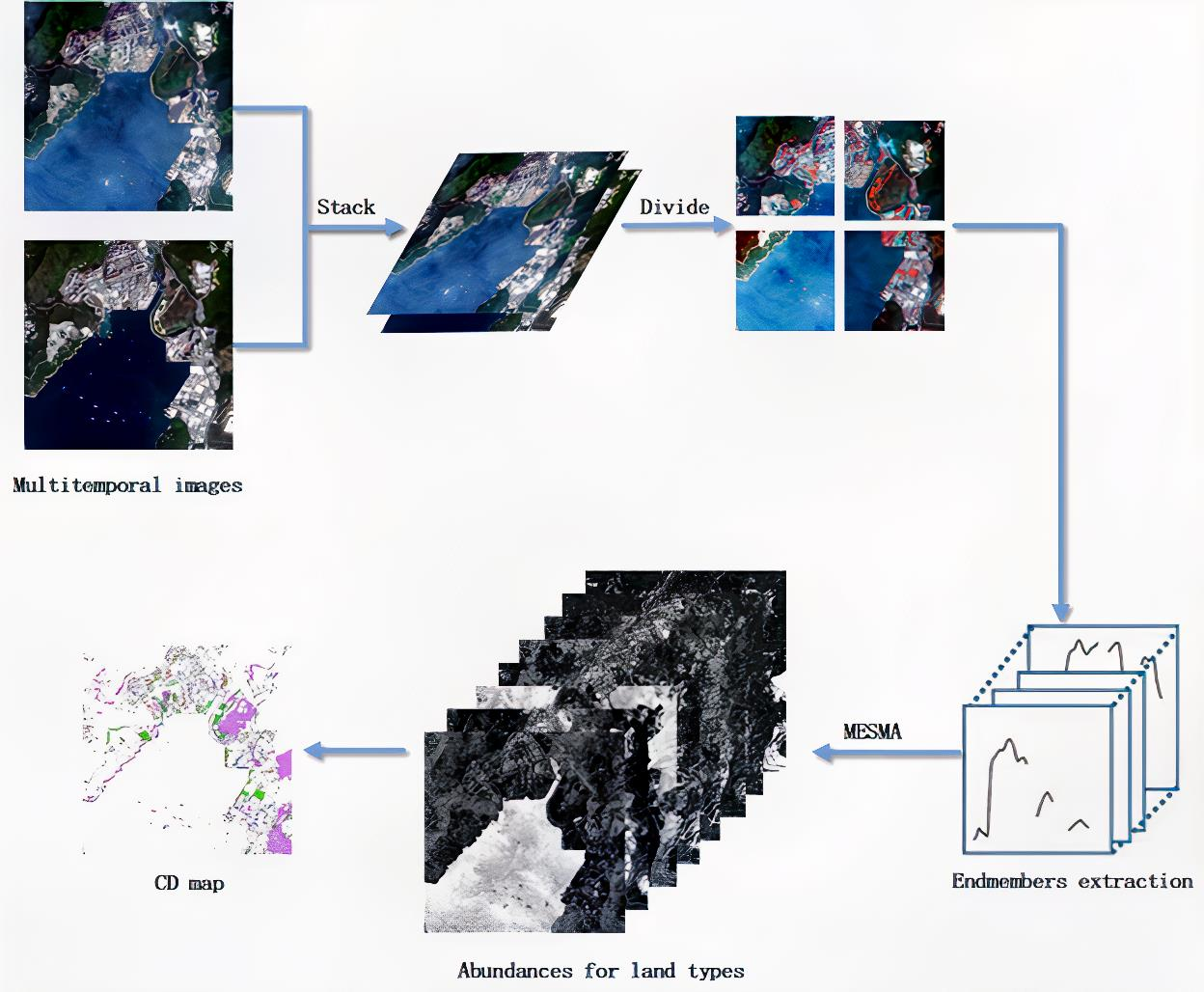
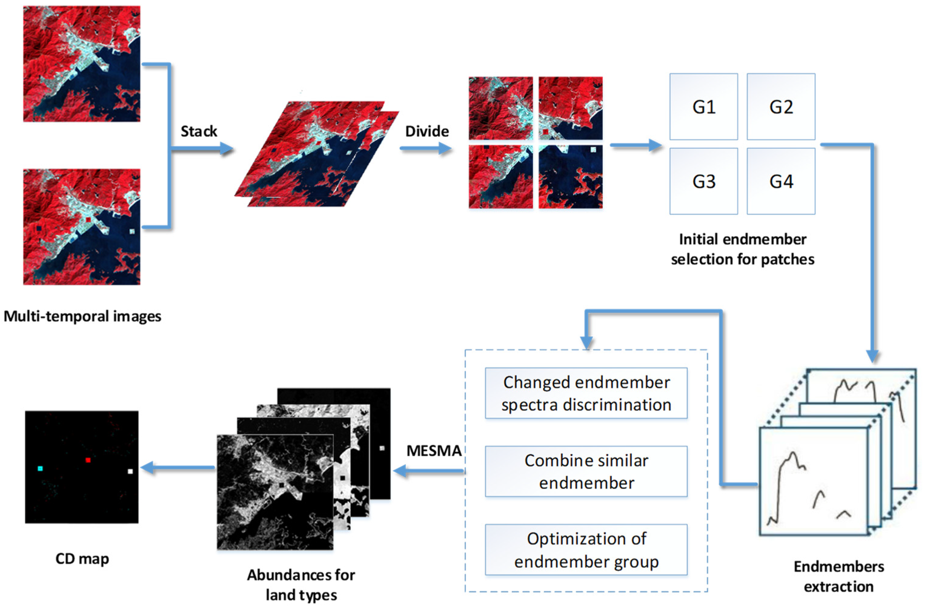
3. The Proposed CD_SDSUVE Algorithm
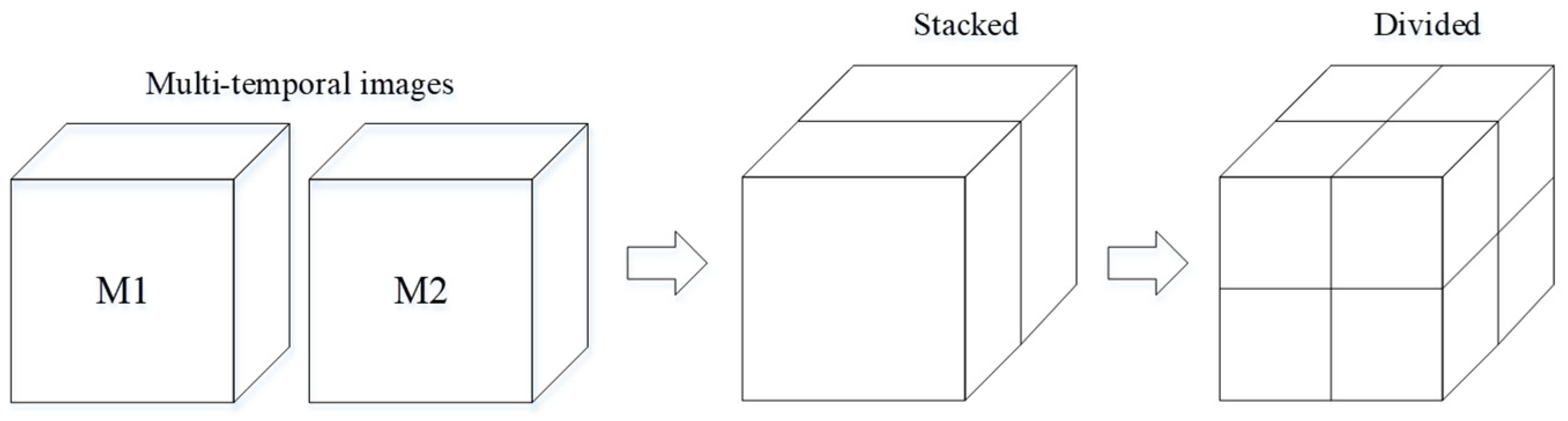
3.1. Stacking and Patch Generation of the Multitemporal Images
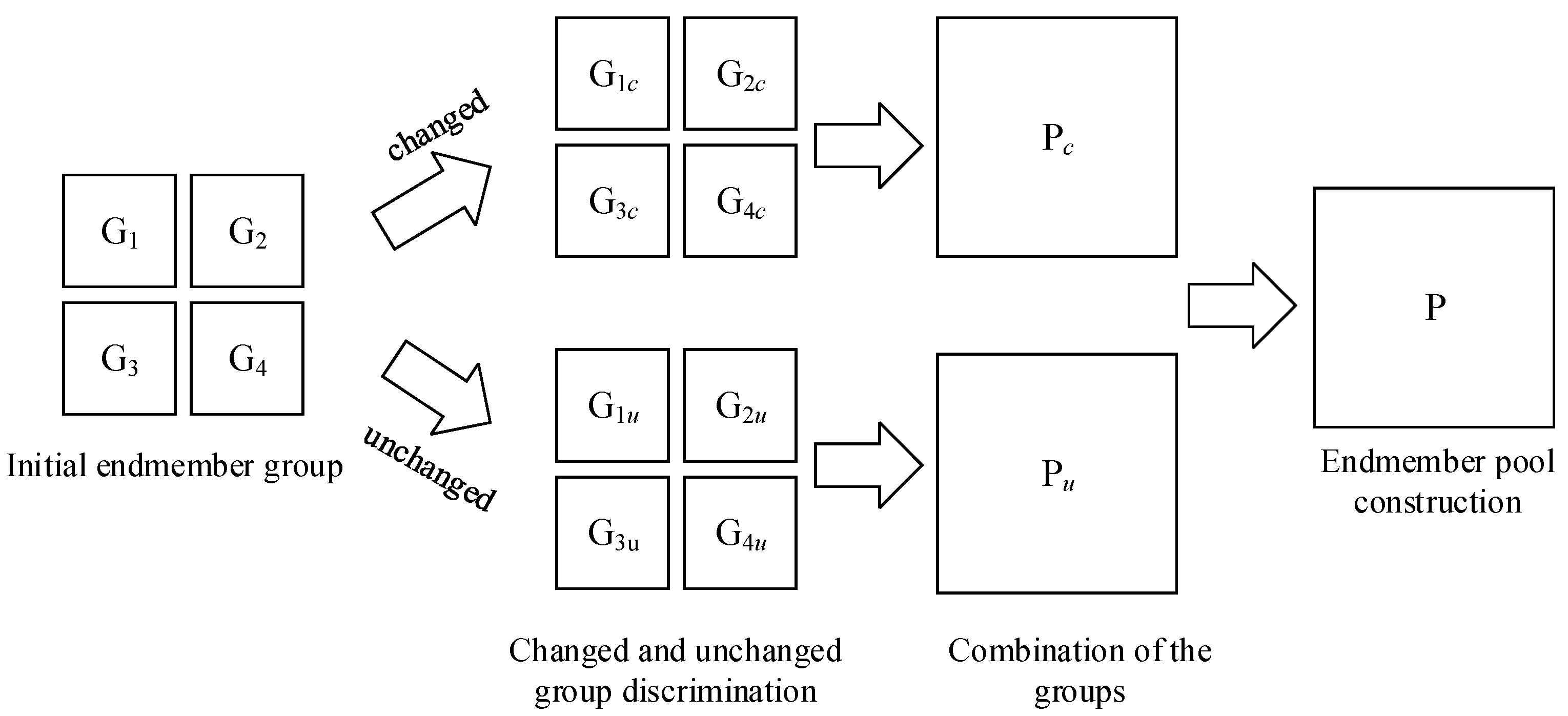
3.2. The Initial Endmember Group Construction for Small Patch Image
3.3. Construction of the Endmember Pool for the Stacked Image
3.4. Multiple Endmember Spectral Mixture Analysis
4. Experiments and Analysis
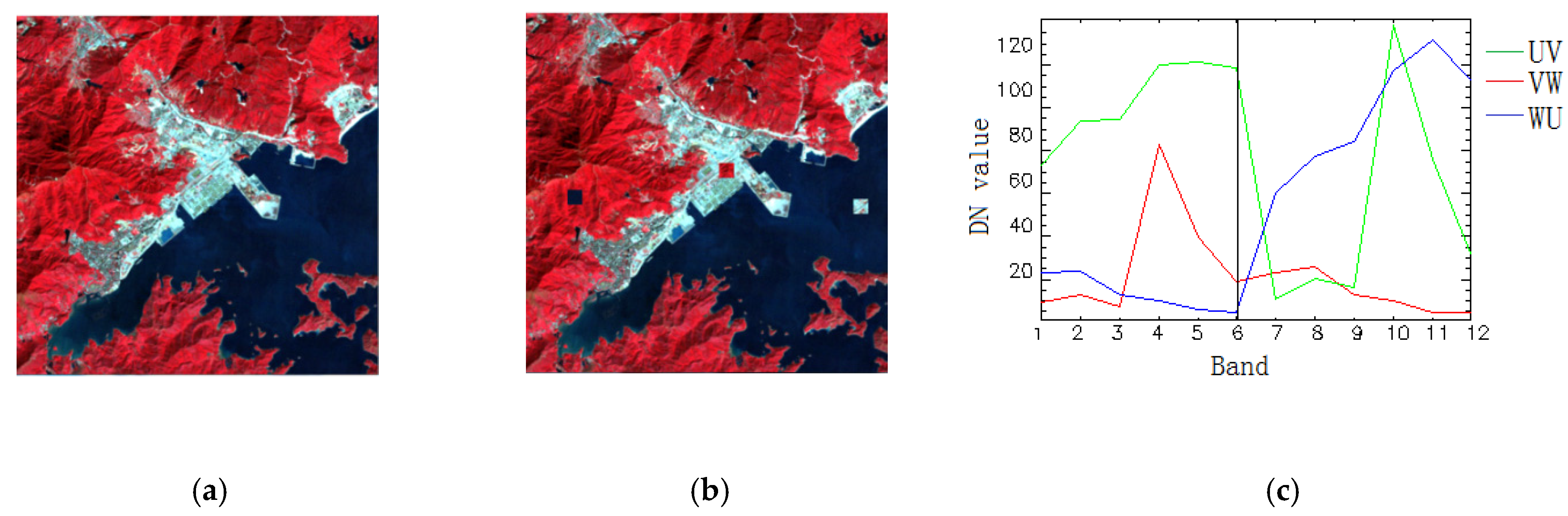
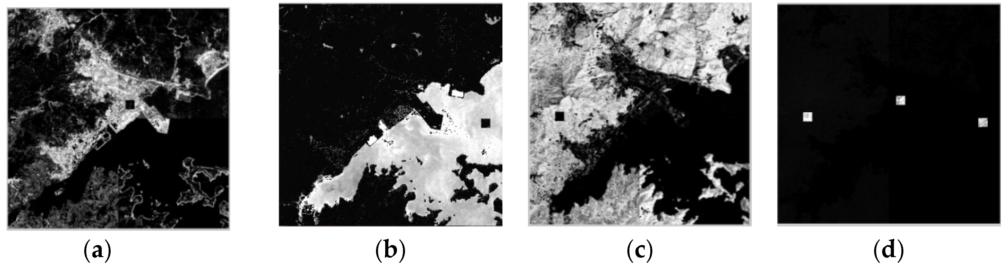
4.1. Simulated Multitemporal Image Data
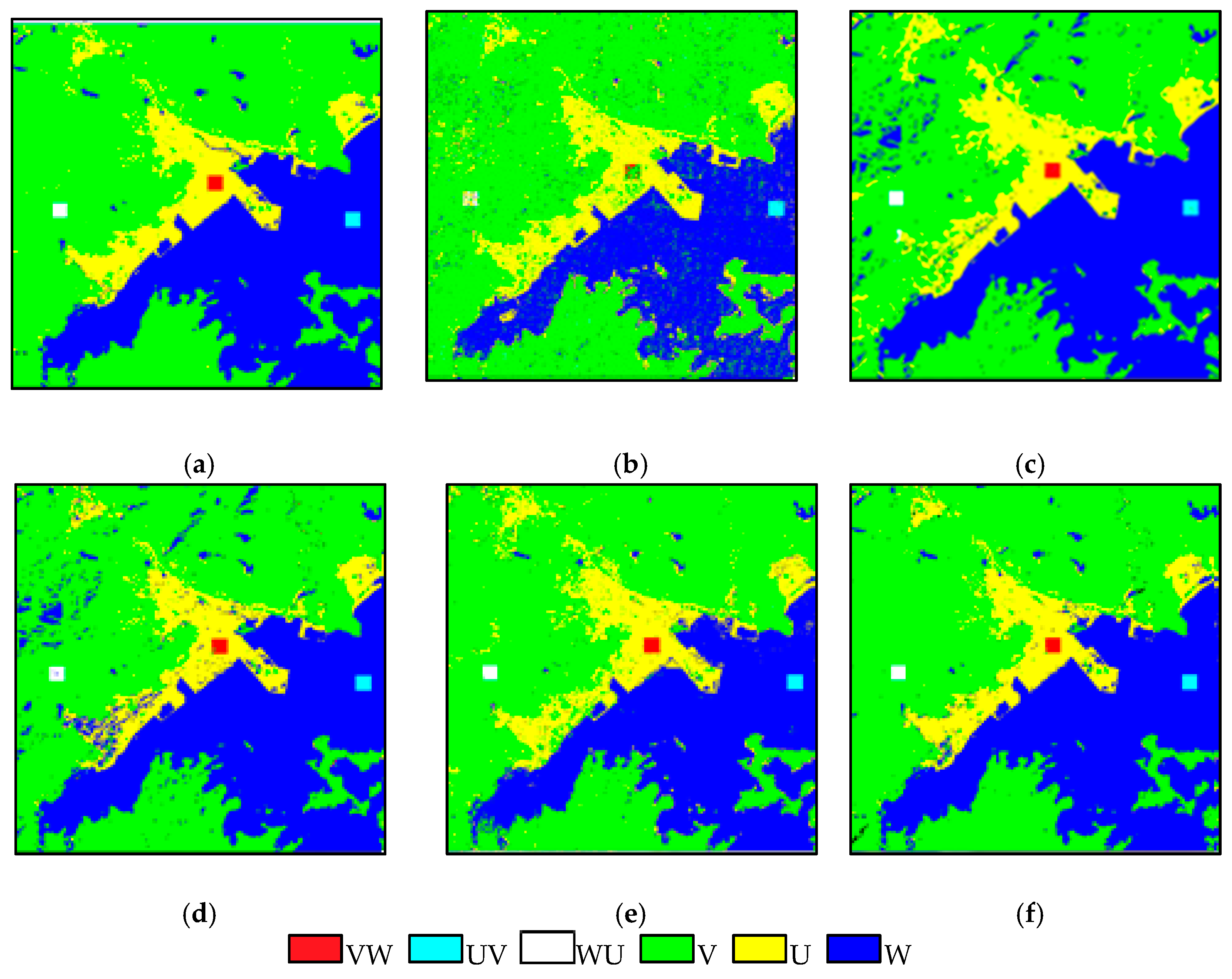
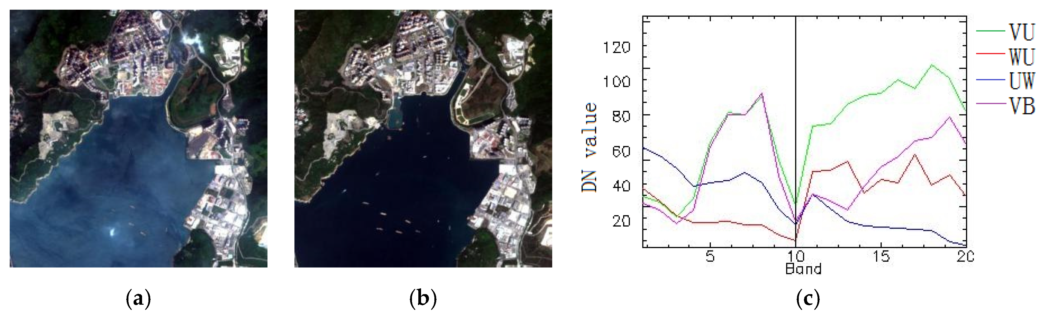
4.2. Real Multitemporal Image Data 1
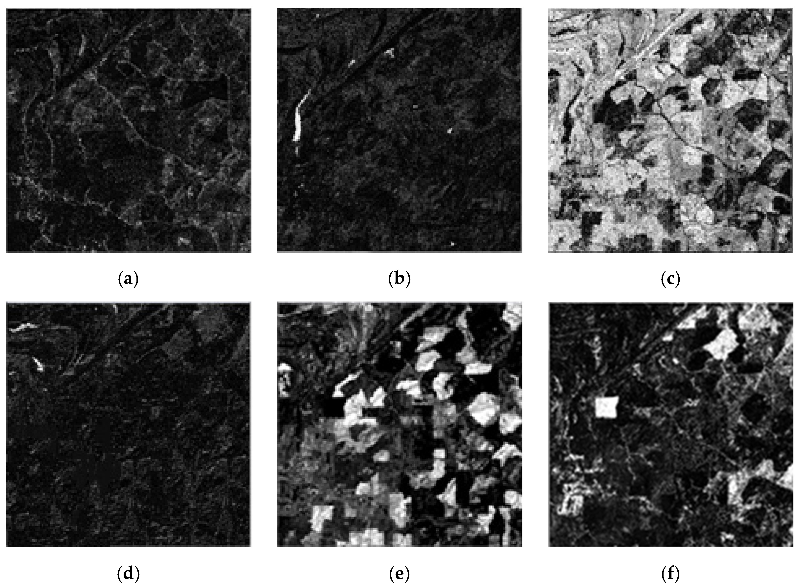
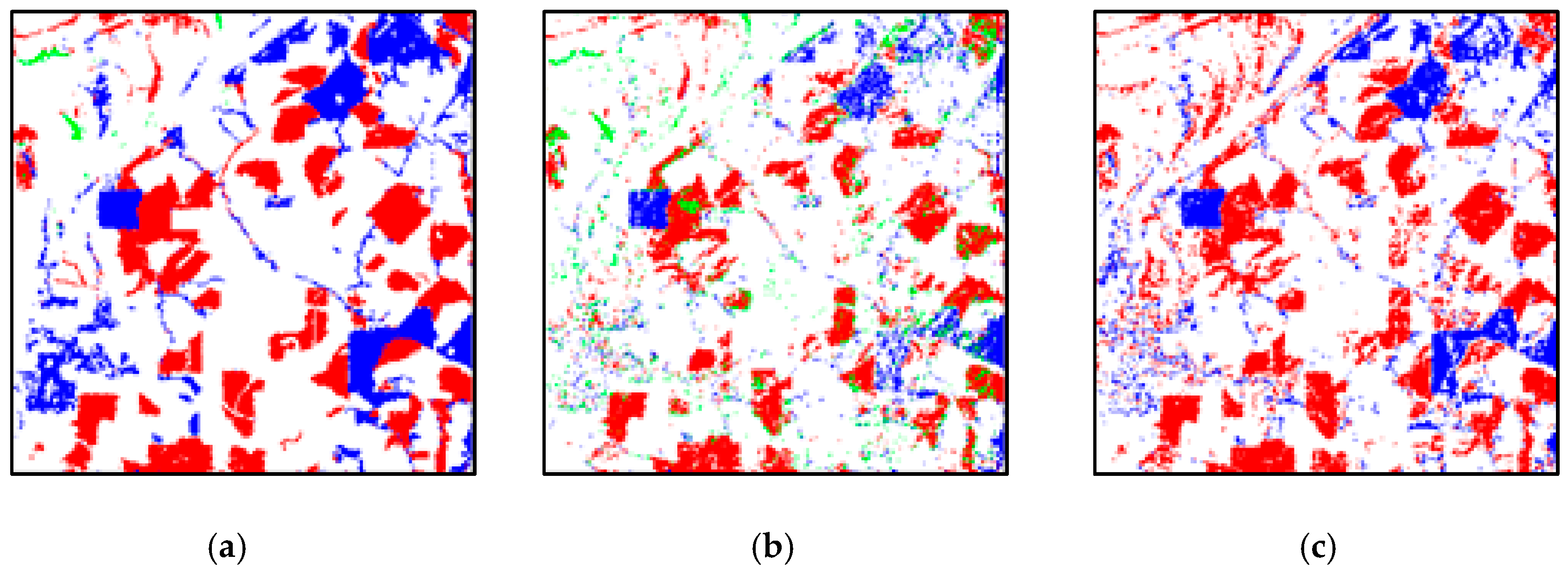
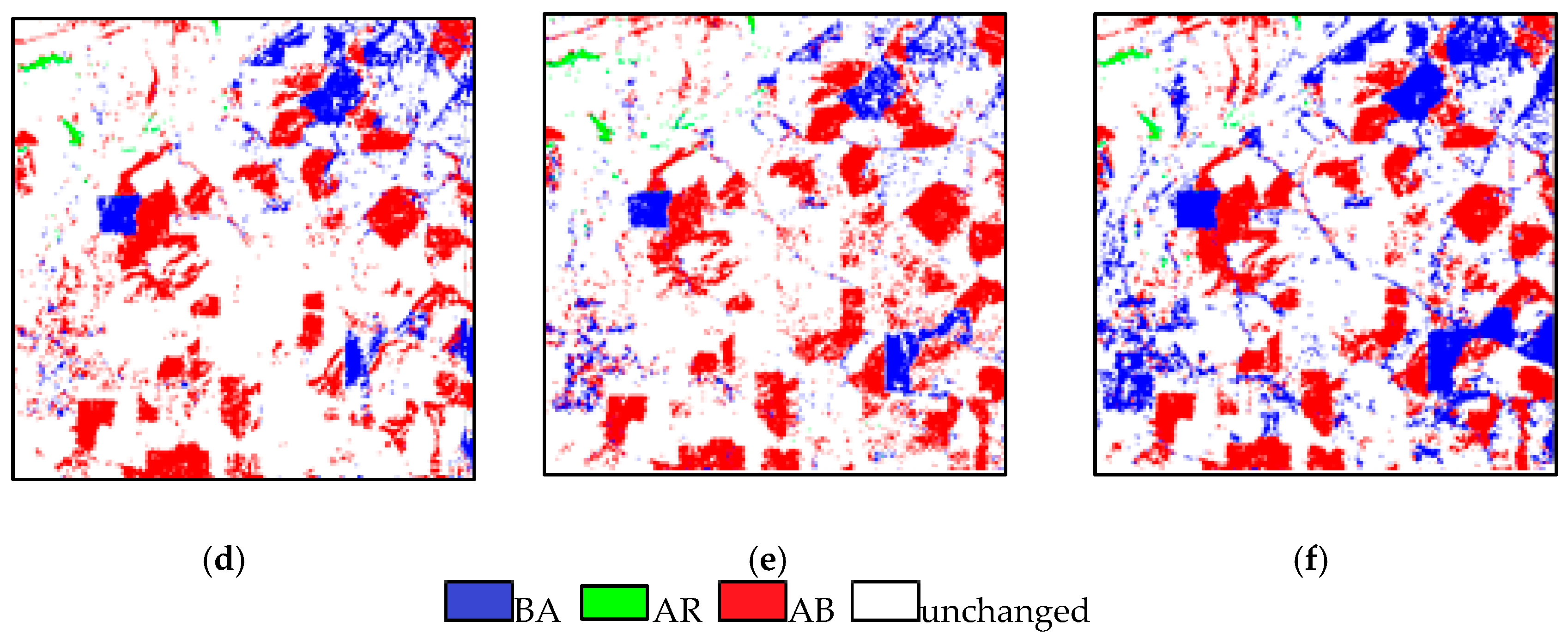
4.3. Real Multitemporal Image Data 2
5. Computational Complexity Analysis
6. Discussion and Conclusions
Author Contributions
Funding
Institutional Review Board Statement
Informed Consent Statement
Data Availability Statement
Acknowledgments
Conflicts of Interest
References
- Coppin, P.; Jonckheere, I.; Nackaerts, K.; Muys, B.; Lambin, E. Review Article Digital change detection methods in ecosystem monitoring: A review. Int. J. Remote Sens. 2004, 25, 1565–1596. [Google Scholar] [CrossRef]
- Zhu, Z.; Woodcock, C.E. Continuous change detection and classification of land cover using all available Landsat data. Remote Sens. Environ. 2014, 144, 152–171. [Google Scholar] [CrossRef] [Green Version]
- Bovolo, F.; Bruzzone, L. A theoretical framework for unsupervised change detection based on change vector analysis in the polar domain. IEEE Trans. Geosci. Remote Sens. 2007, 45, 218–236. [Google Scholar] [CrossRef] [Green Version]
- Gapper, J.J.; El-Askary, H.M.; Linstead, E.; Piechota, T. Coral Reef Change Detection in Remote Pacific Islands Using Support Vector Machine Classifiers. Remote Sens. 2019, 11, 1525. [Google Scholar] [CrossRef] [Green Version]
- Im, J.; Jensen, J.R. A change detection model based on neighborhood correlation image analysis and decision tree classification. Remote Sens. Environ. 2005, 99, 326–340. [Google Scholar] [CrossRef]
- Zong, K.; Sowmya, A.; Trinder, J. Building change detection from remotely sensed images based on spatial domain analysis and Markov random field. J. Appl. Remote. Sens. 2019, 13, 1–9. [Google Scholar] [CrossRef]
- Hong, D.; Yokoya, N.; Chanussot, J.; Zhu, X.X. An Augmented Linear Mixing Model to Address Spectral Variability for Hyperspectral Unmixing. IEEE Trans. Image Proc. 2019, 28, 1923–1938. [Google Scholar] [CrossRef] [Green Version]
- Khelifi, L.; Mignotte, M. Deep learning for change detection in remote sensing images: Comprehensive review and meta-analysis. IEEE Access 2020, 8, 126385–126400. [Google Scholar] [CrossRef]
- Keshava, N.; Mustard, J.F. Spectral unmixing. IEEE Signal Process 2002, 19, 44–57. [Google Scholar] [CrossRef]
- Haertel, V.; Shimabukuro, Y.E.; Almeida-Filho, R. Fraction images in multitemporal change detection. Int. J. Remote Sens. 2004, 25, 5473–5489. [Google Scholar] [CrossRef]
- Anderson, L.O.; Shimabukuro, Y.E.; Arai, E. Cover: Multitemporal fraction images derived from Terra MODIS data for analysing land cover change over the Amazon region. Int. J. Remote Sens. 2005, 26, 2251–2257. [Google Scholar] [CrossRef]
- Zurita-Milla, R.; Gómez-Chova, L.; Guanter, L.; Clevers, J.G.; Camps-Valls, G. Multitemporal unmixing of medium-spatial-resolution satellite images: A case study using meris images for land-cover mapping. IEEE Trans. Geosci. Remote Sens. 2011, 49, 4308–4317. [Google Scholar] [CrossRef]
- Jafarzadeh, H.; Hasanlou, M. An Unsupervised Binary and Multiple Change Detection Approach for Hyperspectral Imagery Based on Spectral Unmixing. IEEE J. Sel. Top. Appl. Earth Obs. Remote Sens. 2020, 12, 4888–4906. [Google Scholar] [CrossRef]
- Gao, Z.H.; Zhang, L.; Li, X.Y.; Liao, M.S.; Qiu, J.Z. Detection and Analysis of Urban Land Use Changes through Multi-temporal Impervious Surface Mapping. Int. J. Remote Sens. 2010, 14, 593–606. [Google Scholar]
- Yang, L.; Xian, G.; Klaver, J.M.; Deal, B. Urban land-cover change detection through sub-pixel imperviousness mapping using remotely sensed data. Photogramm. Eng. Remote Sens. 2003, 69, 1003–1010. [Google Scholar] [CrossRef]
- Somers, B.; Asner, G.P. Multi-temporal hyperspectral mixture analysis and feature selection for invasive species mapping in rainforests. Remote Sens. Environ. 2013, 136, 14–27. [Google Scholar] [CrossRef]
- Du, P.; Liu, S.; Liu, P.; Tan, K.; Cheng, L. Sub-Pixel Change Detection for Urban Land-Cover Analysis via Multi-Temporal Remote Sensing Images. Geo-Spatial Inf. Sci. 2014, 17, 26–38. [Google Scholar] [CrossRef] [Green Version]
- Chen, J.; Chen, X.; Cui, X.; Chen, J. Change vector analysis in posterior probability space: A new method for land cover change detection. IEEE Geosci. Remote Sens. Lett. 2011, 8, 317–321. [Google Scholar] [CrossRef]
- Ling, F.; Foody, G.M.; Ge, Y.; Li, X.; Du, Y. An Iterative Interpolation Deconvolution Algorithm for Superresolution Land Cover Mapping. IEEE Trans. Geosci. Remote Sens. 2016, 54, 7210–7222. [Google Scholar] [CrossRef]
- Jia, S.; Qian, Y. Spectral and Spatial Complexity-Based Hyperspectral Unmixing. IEEE Trans. Geosci. Remote Sens. 2007, 45, 3867–3879. [Google Scholar]
- Lobell, D.B.; Asner, G.P. Cropland distributions from temporal unmixing of MODIS data. Remote Sens. Environ. 2004, 93, 412–422. [Google Scholar] [CrossRef]
- Le Hégarat-Mascle, S.; Seltz, R. Automatic change detection by evidential fusion of change indices. Remote Sens. Environ. 2004, 91, 390–404. [Google Scholar] [CrossRef]
- Wu, K.; Du, Q. Sub-pixel Change Detection of Multi-temporal Remote Sensed Images Using Variability of Endmembers. IEEE Geosci. Remote Sens. Lett. 2017, 14, 796–800. [Google Scholar] [CrossRef]
- Du, Q.; Wasson, L.; King, R. Unsupervised linear unmixing for change detection in multitemporal airborne hyperspectral imagery. In Proceedings of the International Workshop on the Analysis of Multi-Temporal Remote Sensing Images, Biloxi, MI, USA, 16–18 May 2005; pp. 136–140. [Google Scholar]
- Liu, S.; Bruzzone, L.; Bovolo, F.; Du, P. Unsupervised Multitemporal Spectral Unmixing for Detecting Multiple Changes in Hyperspectral Images. IEEE Trans. Geosci. Remote Sens. 2016, 54, 1–16. [Google Scholar] [CrossRef]
- Chen, Z.; Wang, B. Spectrally-spatially regularized low-rank and sparse decomposition: A novel method for change detection in multitemporal hyperspectral images. Remote Sens. 2017, 9, 1044. [Google Scholar] [CrossRef] [Green Version]
- Thompson, D.R.; Mandrake, L.; Gilmore, M.S. Superpixel Endmember Detection. IEEE Trans. Geosci. Remote Sens. 2010, 48, 4023–4033. [Google Scholar] [CrossRef]
- Zhang, L.; Du, B.; Zhong, Y. Hybrid Detectors based on Selective Endmembers. IEEE Trans. Geosci. Remote Sens. 2010, 48, 2633–2646. [Google Scholar] [CrossRef]
- Wang, Q.; Yuan, Z.; Du, Q.; Li, X. GETNET: A General End-to-end Two-dimensional CNN Framework for Hyperspectral Image Change Detection. IEEE Trans. Geosci. Remote Sens. 2019, 57, 3–13. [Google Scholar] [CrossRef] [Green Version]
- Liu, W.; Wu, E.Y. Comparison of non-linear mixture models: Sub-pixel classification. Remote Sens. Environ. 2005, 94, 145–154. [Google Scholar] [CrossRef]
- Heinz, D.C.; Chang, C.-I. Fully constrained least squares linear spectral mixture analysis method for material quantification in hyperspectral imagery. IEEE Trans. Geosci. Remote Sens. 2001, 39, 529–545. [Google Scholar] [CrossRef] [Green Version]
- Luo, B.; Chanussot, J.; Doute, S.; Zhang, L. Empirical automatic estimation of the number of endmembers in hyperspectral images. IEEE Geosci. Remote Sens. Lett. 2013, 10, 24–28. [Google Scholar]
- Wu, K.; Du, Q.; Wang, Y.; Yang, Y. Supervised Sub-Pixel Mapping for Change Detection from Remotely Sensed Images with Different Resolutions. Remote Sens. 2017, 9, 284. [Google Scholar] [CrossRef] [Green Version]
- Alejandra, U.D. Determining the dimensionality of hyperspectral imagery. Master’s Thesis, University of Puerto Rice, San Juan, PR, USA, 2004. [Google Scholar]
- Chan, T.; Chi, C.; Huang, Y.-M.; Ma, W. A convex analysisbased minimum-volume enclosing simplex algorithm for hyperspectral unmixing. IEEE Trans. Signal Process. 2009, 57, 4418–4432. [Google Scholar] [CrossRef]
- Nascimento, J.M.P.; Bioucas-Dias, J.M. Vertex component analysis: A fast algorithm to unmix hyperspectral data. IEEE Trans. Geosci. Remote Sens. 2005, 43, 898–910. [Google Scholar] [CrossRef] [Green Version]
- Lu, D.; Batistella, M.; Moran, E. Multitemporal spectral mixture analysis for Amazonian land-cover change detection. Can. J. Remote Sens. 2004, 30, 87–100. [Google Scholar] [CrossRef]
- Bruzzone, L.; Prieto, D.F. An adaptive semiparametric and context-based approach to unsupervised change detection in multitemporal remote-sensing images. IEEE Trans. Image Process. 2002, 11, 452–466. [Google Scholar] [CrossRef]
- Chen, J.; Wang, R.; Wang, C. Combining magnitude and shape features for hyperspectral classification. Int. J. Remote Sens. 2009, 30, 3625–3636. [Google Scholar] [CrossRef]
- Powell, R.; Roberts, D.; Dennison, P.; Hess, L. Sub-pixel mapping of urban land cover using multiple endmember spectral mixture analysis: Manaus, Brazil. Remote Sens. Environ. 2007, 106, 253–267. [Google Scholar] [CrossRef]
- Quintano, C.; Fernandez-Manso, A.; Roberts, D. Multiple Endmember Spectral Mixture Analysis (MESMA) to map burn severity levels from Landsat images in Mediterranean countries. Remote Sens. Environ. 2013, 136, 76–88. [Google Scholar] [CrossRef]


| Input: Remote Sensing Data: M1 and M2 |
|---|
| Step 1: Two data M1 and M2 are stacked to a new data MS Step 2: Divided scale s is defined, and MS is divided as p (p = s2) patch images Step 3: Initialize the endmember group for ith patch image by N-FINDR Step 4: Analyze each endmember group and generate a whole endmember pool P for the stacked image (1) Discrimination of the changed and unchanged land cover types (2) Combination and analysis of the similar endmember spectrum by SAM (3) The endmember pool is built based on all of the endmember groups Step 5: Construction of multiple endmember spectral unmixing model (1) Select the suitable endmember class using EAR indicator (2) Spectral unmixing with the multiple endmember matrix Step 6: compare the abundance and the final change map is generated Output: The change map of M1 and M2 |
| Class | Number | ||||||
|---|---|---|---|---|---|---|---|
| Group | W | U | V | WU | UV | VW | |
| G1 | 2 | 3 | 3 | 0 | 0 | 1 | |
| G2 | 1 | 3 | 2 | 0 | 3 | 0 | |
| G3 | 2 | 3 | 1 | 0 | 0 | 1 | |
| G4 | 1 | 3 | 2 | 3 | 0 | 0 | |
| Method | CD_PC | CD_SU | CD_SSU | CD_SDSU | CD_SDSUVE |
|---|---|---|---|---|---|
| OA | 88.09% | 93.83% | 94.07% | 97.53% | 99.61% |
| Kappa | 0.76 | 0.91 | 0.91 | 0.96 | 0.99 |
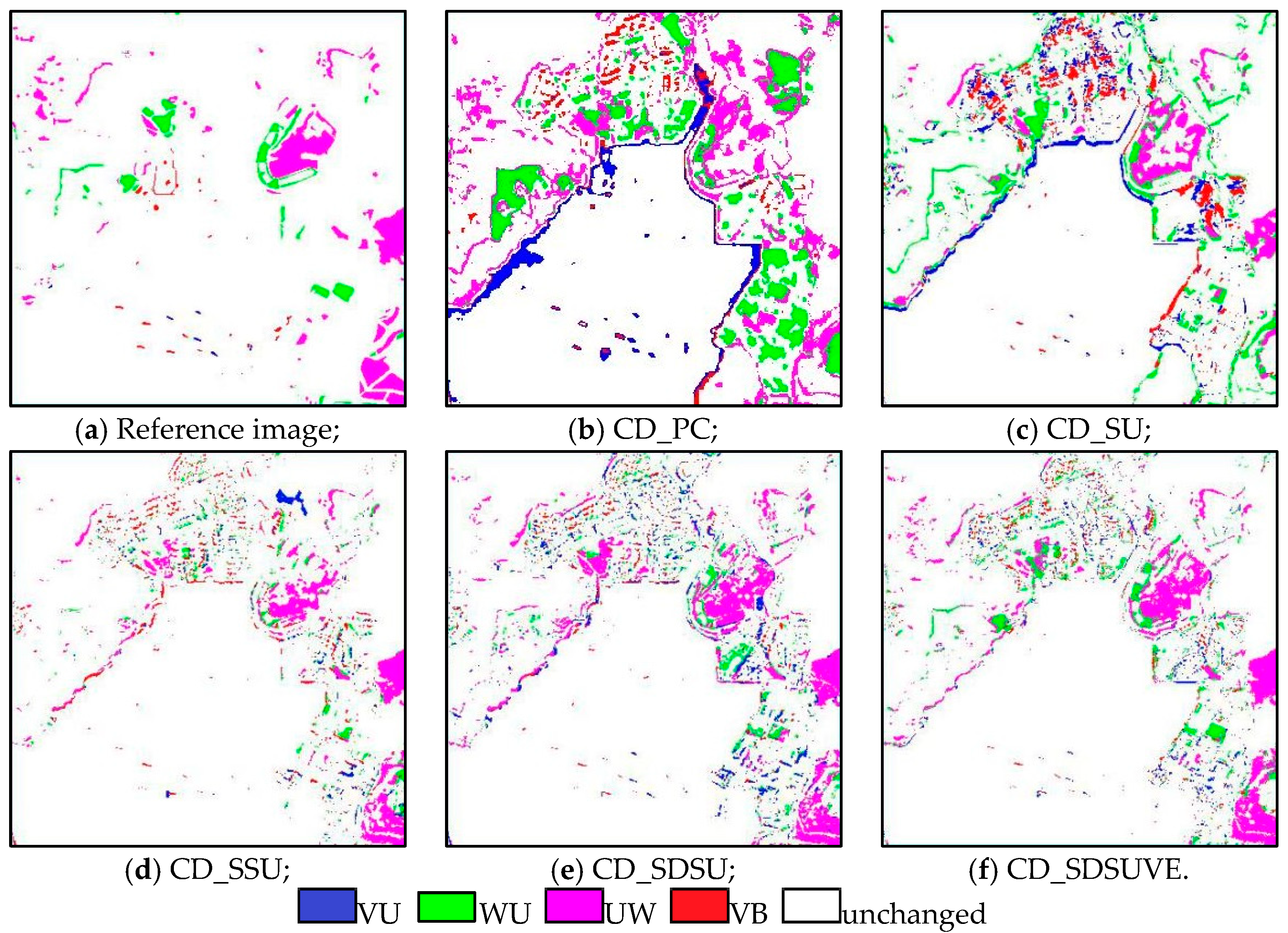
| Class | Number | ||||||||
|---|---|---|---|---|---|---|---|---|---|
| Group | U | V | B | W | VU | VB | WU | UW | |
| G1 | 5 | 3 | 1 | 1 | 3 | 2 | 2 | 0 | |
| G2 | 4 | 3 | 2 | 1 | 2 | 3 | 1 | 0 | |
| G3 | 3 | 2 | 1 | 2 | 1 | 2 | 2 | 1 | |
| G4 | 5 | 2 | 2 | 2 | 2 | 2 | 1 | 2 | |
| Method | CD_PC | CD_SU | CD_SSU | CD_SDSU | CD_SDSUVE |
|---|---|---|---|---|---|
| OA | 78.38% | 87.41% | 92.82% | 91.35% | 93.26% |
| Kappa | 0.44 | 0.58 | 0.59 | 0.64 | 0.66 |
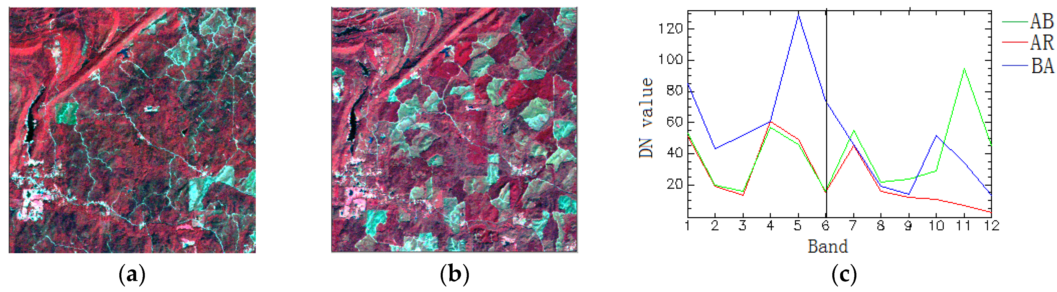
| Class | Number | ||||||
|---|---|---|---|---|---|---|---|
| Group | B | R | A | AR | AB | BA | |
| G1 | 3 | 2 | 2 | 3 | 1 | 1 | |
| G2 | 2 | 3 | 2 | 2 | 1 | 2 | |
| G3 | 4 | 3 | 3 | 0 | 0 | 2 | |
| G4 | 5 | 3 | 3 | 0 | 2 | 1 | |
| G5 | 2 | 3 | 2 | 3 | 2 | 0 | |
| G6 | 3 | 3 | 2 | 1 | 1 | 2 | |
| G7 | 3 | 2 | 3 | 0 | 2 | 2 | |
| G8 | 2 | 3 | 3 | 0 | 2 | 2 | |
| G9 | 3 | 3 | 3 | 1 | 1 | 1 | |
| Method | CD_PC | CD_SU | CD_SSU | CD_SDSU | CD_SDSUVE | |
|---|---|---|---|---|---|---|
| Omission Error | AR | 91.4% | 25.1% | 7.4% | 6.1% | 5.4% |
| AB | 9.6% | 27.8% | 7.9% | 8.8% | 7.3% | |
| BA | 9.4% | 37.9% | 19.9% | 17.9% | 9.1% | |
| Commission Error | AR | 40.8% | 18.5% | 16.1% | 16.4% | 13.5% |
| AB | 22.2% | 22.9% | 17.5% | 18.7% | 15.3% | |
| BA | 16.3% | 25.5% | 13.4% | 22.8% | 10.0% | |
| OA | 67.43% | 72.43% | 73.36% | 76.13% | 80.85% | |
| Kappa | 0.31 | 0.46 | 0.47 | 0.48 | 0.56 | |
| Time (ms) | CD_PC | CD_SU | CD_SSU | CD_SDSU | CD_SDSUVE |
|---|---|---|---|---|---|
| Simulated data | 1410 | 1504 | 780 | 4126 | 7862 |
| Real data 1 | 1486 | 1513 | 981 | 4772 | 7985 |
| Real data 2 | 1517 | 1589 | 1240 | 5639 | 9623 |
Publisher’s Note: MDPI stays neutral with regard to jurisdictional claims in published maps and institutional affiliations. |
© 2021 by the authors. Licensee MDPI, Basel, Switzerland. This article is an open access article distributed under the terms and conditions of the Creative Commons Attribution (CC BY) license (https://creativecommons.org/licenses/by/4.0/).
Share and Cite
Wu, K.; Chen, T.; Xu, Y.; Song, D.; Li, H. A Novel Change Detection Approach Based on Spectral Unmixing from Stacked Multitemporal Remote Sensing Images with a Variability of Endmembers. Remote Sens. 2021, 13, 2550. https://0-doi-org.brum.beds.ac.uk/10.3390/rs13132550
Wu K, Chen T, Xu Y, Song D, Li H. A Novel Change Detection Approach Based on Spectral Unmixing from Stacked Multitemporal Remote Sensing Images with a Variability of Endmembers. Remote Sensing. 2021; 13(13):2550. https://0-doi-org.brum.beds.ac.uk/10.3390/rs13132550
Chicago/Turabian StyleWu, Ke, Tao Chen, Ying Xu, Dongwei Song, and Haishan Li. 2021. "A Novel Change Detection Approach Based on Spectral Unmixing from Stacked Multitemporal Remote Sensing Images with a Variability of Endmembers" Remote Sensing 13, no. 13: 2550. https://0-doi-org.brum.beds.ac.uk/10.3390/rs13132550