Improvement of UAV Positioning Performance Based on EGNOS+SDCM Solution

Abstract

The article presents the results of research on multi-SBAS (multi-satellite-based augmentation system) positioning in UAV (unmanned aerial vehicle) technology. For this purpose, a new solution was developed for combining the UAV position navigation solution from several SBAS systems. In this particular case, the presented linear combination algorithm is based on the fusion of EGNOS (European geostationary navigation overlay service) and SDCM (system of differential correction and monitoring) positioning to determine the resultant UAV coordinates. The algorithm of the mathematical model uses weights of measurements in three ways, i.e., Variant I, the reciprocal of the number of tracked satellites from a single SBAS solution; Variant II, the inverse square of mean coordinate errors from a single SBAS solution; and Variant III, the reciprocal of UAV flight speed from a single SBAS solution. The research experiment used real GNSS (global navigation satellite system) navigation data recorded by the VTOL unmanned platform. The test flight was made in April 2020 in Poland, near Warsaw. Based on the developed research results, it was found that the highest accuracy of UAV positioning was obtained when using the weighting model for Variant II. In the weight model of Variant II, the accuracy of the solution of the UAV position increased by 1–2% for the horizontal components and 19–22% for the vertical component h, concerning the results obtained from the weighing Variants I and III. It is worth noting that the proposed research model significantly improves the results of determining the ellipsoidal height h. Compared to the arithmetic mean model, determining the h component in the Variant II weight model is improved by about 23%. The paper also shows the advantage of EGNOS+SDCM positioning over EGNOS positioning alone in determining the accuracy of the vertical component h. The obtained research results show the significant advantages of the multi-SBAS positioning model in UAV technology.

1. Introduction

In air navigation, an increasing number of operations are performed with the use of UAVs (unmanned aerial vehicles) [1]. Therefore, more accurate navigation solutions are needed to determine the position of the UAV. Of course, most UAVs are equipped with single-frequency GNSS receivers (global navigation satellite system) [2,3], which provide positioning accuracy of up to 10 m or better [4]. However, new solutions are necessary to implement to ensure effective improvement of the determined UAV coordinates. One solution, a simple ratio in implantation, is the use of SBAS (satellite-based augmentation system) [5] corrections to improve the UAV positioning performance. The process of using SBAS corrections causes modification of the observation equation in the SPP (single point positioning) coding method [6]. It means that the following parameters in the observation equation of the RMS method are corrected [7]:

-

the position of the GNSS satellite is corrected with SBAS corrections;

-

the GNSS satellite clock error is corrected with SBAS corrections;

-

the ionospheric delay is determined from the SBAS model [8];

-

the tropospheric delay is determined from the RTCA-MOPS model (Radio Technical Commission for Aeronautics—Minimum Operational Performance Specification) [9,10].

Therefore, it can be concluded that SBAS corrections allow the modification of four parameters in the observation equation of the SPP method. That, in turn, translates into improved performance of the determined UAV coordinates and an increase in the accuracy of UAV positioning. Searching for new navigation solutions for UAV technology using SBAS corrections may turn out to be an excellent move, even more so as the SBAS solution can significantly improve the accuracy of the positioning of the UAV to the results obtained with the differential technique RTK-OTF (real-time kinematic—on the fly) [11].

2. Related Works

The current research trend and directions of scientific work on the application of SBAS in UAV technology mainly concern:

-

the use of the SBAS solution in UAV technology to perform VLOS (visual line of sight) and BVLOS (beyond visual line of sight) flights [12];

-

the determination of SBAS EGNOS (European Geostationary Navigation Overlay Service) positioning reliability for UAV technology [13];

-

the implementation of the SBAS solution in aviation operations performed in circumpolar zones with the use of UAV technology [14];

-

the application of SBAS solutions for RPAS systems (Remotely Piloted Aircraft Systems) [15];

-

the use of SBAS to determine the approximate values of external orientation elements for low-level photogrammetry [16,17];

-

the use of the SBAS system in UAV technology to support the SAR (search and rescue) system [18,19,20];

-

the use of the SBAS solution for precise UAV positioning in real-time and post-processing mode [21];

-

the use of the SBAS system in UAV positioning during the landing approach procedure [22,23];

-

the UAV positioning using SBAS corrections as part of the PBN (performance-based navigation) navigation concept [24].

The research mentioned above [12,13,14,15,16,17,18,19,20,21,22,23,24] concerned mainly a single SBAS augmentation system, e.g., the EGNOS system [25]. The following research problem arises regarding positioning a moving object (e.g., UAV) using a navigation solution from several SBAS assistance systems. This approach is referred to in the literature as multi-SBAS positioning. In the scientific literature, examples of research work on multi-SBAS positioning can be found. The work [26] shows the current state of knowledge concerning the application of SBAS augmentation systems for the area of Japan, mainly the MSAS (MTSAT-based augmentation system) and QZSS (quasi-zenith satellite system) augmentation systems. In particular, it was shown how the MSAS system improves the GPS (global positioning system) autonomous positioning and the possibilities of using SBAS corrections in the QZSS system on the L5 frequency. In turn, work [27] shows a scheme of connecting the position navigation solution in the Singapore area to the MSAS and GAGAN (GPS aided geo augmented navigation) support systems. In particular, corrections from MSAS+GAGAN systems were used to improve GPS positioning in the Singapore area. Moreover, paper [28] shows the possibility of using the SBAS positioning function for Airbus aircraft during test flights. On-board instrumentation type A350 XWB with SBAS positioning function allows corrections from EGNOS, MSAS, and WAAS (wide-area augmentation system) assistance systems. The work mainly shows the possibilities of interoperability between individual SBAS systems for Airbus aircraft. Another publication [29] presented a new model of the SBAS ionosphere for the integration of WAAS and MSAS measurements. The ionospheric grid points model is based on a regular grid of squares with IGP nodes (ionospheric grid points). At each grid node, there is a defined VTEC (vertical TEC) ionospheric delay. In the proposed ionospheric model, the VTEC values are interpolated from a minimum of four IGP knots to determine the resultant ionospheric delay value for a given geodetic latitude and longitude. Moreover, the applied SBAS ionosphere model will be used in the KAAS augmentation system (Korea Augmentation Satellite System). The paper [30] presents fascinating research results concerning the development of a standard SBAS correction format and signal for BDSBAS (BeiDou SBAS), WAAS, EGNOS, GAGAN, QZSS, MSAS, and SDCM (system of differential correction and monitoring) systems with global satellite navigation systems GNSS. This solution is used to increase the interoperability and compatibility of global GNSS systems with SBAS augmentation systems. The publication [31] shows the use of multi-SBAS corrections in multi-GNSS positioning. In particular, MSAS and SDCM fixes were used to improve GPS and GPS/GLONASS positioning. In turn, the article [32] shows the results of determining the reliability levels HPL (horizontal protection level) and VPL (vertical protection level) for positioning in various configurations for typical aviation applications. The research used corrections from SBAS satellites numbered 120–158. The obtained test results were compared with the performance of the LPV-200 landing approach (localizer performance with vertical guidance—200) according to the ICAO (International Civil Aviation Organization) requirements. In work [33], scientific research was carried out on the determination of the orbit and clock error of the GPS satellite after taking into account the WASS, EGNOS, and SDCM corrections for precise point positioning (PPP) in the GPS. However, in [34], corrections were made to the position of the GPS satellite and the error of the GPS satellite clock and the ionospheric delay with the use of corrections from the WAAS, SDCM, GAGAN, MSAS, and EGNOS systems. Based on the studied literature [25,26,27,28,29,30,31,32,33,34], various aspects of the multi-SBAS positioning were shown. The multitude of SBAS assistance systems is interesting from the point of view of combining and fusing single-position navigation solutions, including the position of the UAV. For UAV technology, the multi-SBAS solution can primarily improve positioning accuracy. Especially the aspect of improving the value of the vertical h component seems to be of crucial importance for the stabilization of the UAV flight. Therefore, the paper proposes a new solution for improving UAV coordinates based on the multi-SBAS positioning ideas. Namely, the paper proposes a linear combination model to determine the resultant UAV position based on a single navigation solution using corrections from the EGNOS and SDCM systems. Real GNSS measurement data acquired by the UAV platform and EGNOS+SDCM corrections were used in the presented work. The presented model is unique because it is based on three different weighting variants in a linear combination of the weighted average model. The weighting as a function was proposed:

-

the reciprocal of the number of tracked satellites from a single SBAS solution;

-

the inverse of the square of the mean coordinate errors from a single SBAS solution;

-

the reciprocal of the UAV flight speed from a single SBAS solution.

This approach is interesting because it depends on the positioning process itself—the number of satellites tracked on the stochastic process of a single SBAS solution—on the meaning of the mean coordinate errors, and on the navigation and piloting of the UAV flight itself—read UAV flight speed. Therefore, the proposed research topic goes beyond the available scientific literature [12,13,14,15,16,17,18,19,20,21,22,23,24,25,26,27,28,29,30,31,32,33,34]. The developed research methodology and the obtained research results can be directly implemented in UAV technology in GNSS positioning.

The linear combination model in the form of a weighted average method has already been used in air navigation.

Table 1. The characteristic of the mean weighted model in research work in the aeronautical area.

Vehicle	Navigational Parameter	Mean Weighted Model	Assessment
UAV [7]	Resultant coordinates BLh of UAV [7]	Measurement weights were defined as the inverse of the squared mean error values of the determined coordinates [7]	Standard deviation of the UAV position calculated from the weighted mean model improved by about 21 ÷ 50% compared to the arithmetic mean model’s solution [7]
Aircraft [35]	Resultant coordinates XYZ of aircraft vehicle [35]	The measurement weights are a function of the number of GPS and GLONASS satellites and the inverse of the mean error square [35]	The obtained accuracy is better by 11–87% for the model with a weighting scheme as a function of the inverse of the mean error square [35]
Aircraft [36]	Resultant velocity of aircraft vehicle [36]	Measurement weights were defined as the inverse number of GNSS satellites [36]	The RMS error of resultant velocity is less than 0.05 m/s [36]
Aircraft [37]	Resultant coordinates XYZ of aircraft vehicle [37]	Measurement weights were used as a function of the number of GPS satellites being tracked, and geometric PDOP (position dilution of precision) coefficient [37]	The RMS (root mean square) accuracy of positioning for XYZ geocentric coordinates was better than 1.2% to 33.7% for the weighted average method compared to a single GPS SPP solution [37]

describes selected research works in which a weighted average model was used to determine the position of an aircraft. Among the works mentioned [7,35,36,37], the weighted average model was based on one or two measuring weights. On the other hand, the presented article shows a weighing scheme for three different weighing scales. Moreover, in the works [7,35,36,37], the experiment used satellite data in the GPS, EGNOS, and GPS/GLONASS systems. On the other hand, the presented work presents a weighted average model for two support systems, SDCM and EGNOS. As for the vehicle used in the experiment, it is worth emphasizing that the research tests relate to the aircraft or UAV.

In summary, the main achievements at work are:

-

development of a new linear combination model for the combination of a single SBAS solution from EGNOS and SDCM systems;

-

implementation of various weighing variants in order to optimize the calculation process and selection of the best method to improve the positioning accuracy of the multi-SBAS;

-

development of algorithms for assessing internal and external accuracy;

-

research on improving the determination of the vertical h component for the UAV flight.

3. Research Method

The research methodology is based on the assumption of the integration of UAV positions based on the solution of EGNOS [38] and SDCM positions [39]. This integration of navigation data should be based on a weight model. Weighing of measurements should be carried out to combine the results of UAV coordinates from the EGNOS and SDCM solution. In the analysed example, it was proposed to use the weighted average model, taking into account the following measuring weights:

-

reciprocal of the number of tracked satellites from a single SBAS solution;

-

the inverse of the square of the mean coordinate errors from a single SBAS solution;

-

the reciprocal of the UAV flight speed from a single SBAS solution.

On this basis, the mathematical model for determining the resultant UAV position will look like this:

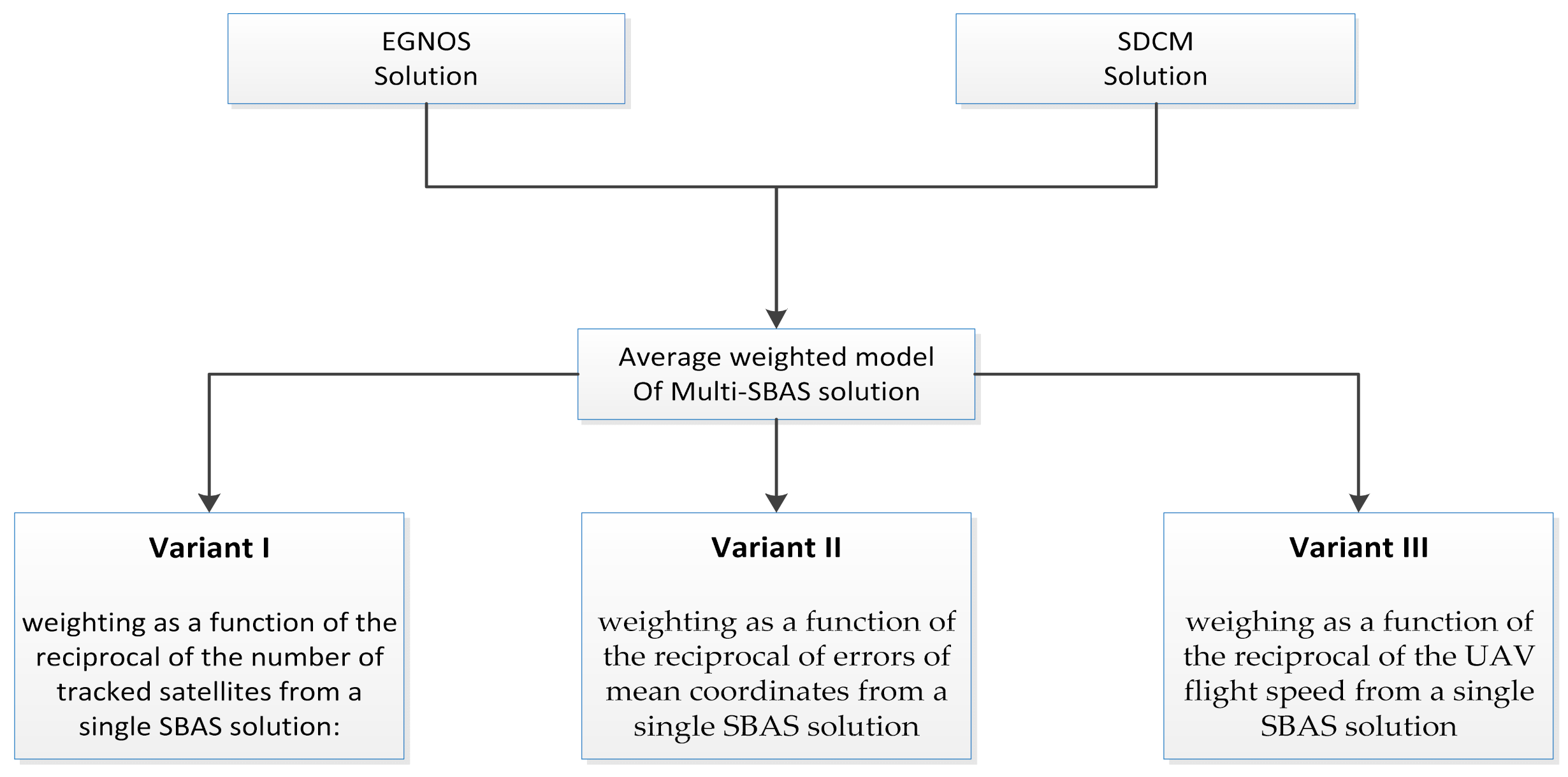
- Variant I weighting as a function of the reciprocal of the number of tracked satellites from a single SBAS solution:

$$\left\{\begin{array}{c}Bm=\frac{\sum w_i·B_i}{\sum w_i}=\frac{\sum \frac{1}{N{s}_i}·B_i}{\sum \frac{1}{N{s}_i}}\\ Lm=\frac{\sum w_i·L_i}{\sum w_i}=\frac{\sum \frac{1}{N{s}_i}·L_i}{\sum \frac{1}{N{s}_i}}\\ hm=\frac{\sum w_i·h_i}{\sum w_i}=\frac{\sum \frac{1}{N{s}_i}·h_i}{\sum \frac{1}{N{s}_i}}\end{array}\right.$$

(1)

where:

$Bm$—resultant latitude;

$Lm$—resultant longitude;

$hm$—resultant ellipsoidal height;

$w$—measure weight;

$i$—SBAS single solution index, i.e., EGNOS and SDCM;

$N{s}_i$—number of satellites from a single SBAS solution (EGNOS and SDCM);

$B_i$—geodetic width from a single SBAS solution (EGNOS and SDCM);

$L_i$—geodetic length from a single SBAS solution (EGNOS and SDCM);

$h_i$—ellipsoidal height from a single SBAS solution (EGNOS and SDCM).

Expressing Equation (1) with the use of indices defining the EGNOS solution and SDCM, the algorithm for determining the resultant position of the UAV will take the form:

$$\left\{\begin{array}{c}Bm=\frac{\frac{1}{N{s}_E}·B_E+\frac{1}{N{s}_S}·B_S}{\frac{1}{N{s}_E}+\frac{1}{N{s}_S}}\\ Lm=\frac{\frac{1}{N{s}_E}·L_E+\frac{1}{N{s}_S}·L_S}{\frac{1}{N{s}_E}+\frac{1}{N{s}_S}}\\ hm=\frac{\frac{1}{N{s}_E}·h_E+\frac{1}{N{s}_S}·h_S}{\frac{1}{N{s}_E}+\frac{1}{N{s}_S}}\end{array}\right.$$

(2)

where:

$N{s}_E$—number of satellites from the EGNOS solution;

$N{s}_S$—number of satellites from the SDCM solution;

$B_E$—geodetic width from the EGNOS solution;

$B_S$—geodetic width from the SDCM solution;

$L_E$—geodetic length from the EGNOS solution;

$L_S$—geodetic length from the SDCM solution;

$h_E$—ellipsoidal height from the EGNOS solution;

$h_S$—ellipsoidal height from SDCM solution.

- Variant II weighting as a function of the reciprocal of errors of mean coordinates from a single SBAS solution:

$$\left\{\begin{array}{c}Bm=\frac{\sum w_i·B_i}{\sum w_i}=\frac{\sum \frac{1}{{C{l}^2}_i}·B_i}{\sum \frac{1}{{C{l}^2}_i}}\\ Lm=\frac{\sum w_i·L_i}{\sum w_i}=\frac{\sum \frac{1}{{C{l}^2}_i}·L_i}{\sum \frac{1}{{C{l}^2}_i}}\\ hm=\frac{\sum w_i·h_i}{\sum w_i}=\frac{\sum \frac{1}{{C{l}^2}_i}·h_i}{\sum \frac{1}{{C{l}^2}_i}}\end{array}\right.$$

(3)

where:

$C{l}_i$—mean coordinate errors from a single SBAS solution (EGNOS and SDCM).

The mean errors are determined according to [7,40]:

$$C{l}_i^2=\left\{\begin{array}{c}m{B}_i^2 along B axis\\ m{L}_i^2 along L axis\\ m{h}_i^2 along h axis\end{array}\right.$$

(4)

where:

$m{B}_i$—mean errors in determining the geodetic latitude from the SBAS solution (EGNOS and SDCM);

$m{L}_i$—mean errors in determining the geodetic length from the SBAS solution (EGNOS and SDCM);

$m{h}_i$—mean errors of ellipsoidal height determination from SBAS solution (EGNOS and SDCM).

Sequentially substituting the parameters of Equation (4) into the mathematical expression (3) to determine the position of the resultant UAV using the weight measured as the inverse of the average error of coordinate SBAS single solution, we obtain:

$$\left\{\begin{array}{c}Bm=\frac{\frac{1}{{m{B}^2}_E}·B_E+\frac{1}{{m{B}^2}_S}·B_S}{\frac{1}{{m{B}^2}_E}+\frac{1}{{m{B}^2}_S}}\\ Lm=\frac{\frac{1}{{m{B}^2}_E}·L_E+\frac{1}{{m{B}^2}_S}·L_S}{\frac{1}{{m{B}^2}_E}+\frac{1}{{m{B}^2}_S}}\\ hm=\frac{\frac{1}{{m{B}^2}_E}·h_E+\frac{1}{{m{B}^2}_S}·h_S}{\frac{1}{{m{B}^2}_E}+\frac{1}{{m{B}^2}_S}}\end{array}\right.$$

(5)

where:

$m{B}_E$—mean errors in determining the geodetic latitude from the EGNOS solution;

$m{L}_E$—mean errors in determining the geodetic length from the EGNOS solution;

$m{h}_E$—mean errors in the determination of the ellipsoidal height from the EGNOS solution;

$m{B}_S$—mean errors in determining the geodetic latitude from the SDCM solution;

$m{L}_S$—mean errors in determining the geodetic length from the SDCM solution;

$m{h}_S$—mean errors of the determination of the ellipsoidal height from the SDCM solution.

- Variant III weighing as a function of the reciprocal of the UAV flight speed from a single SBAS solution:

$$\left\{\begin{array}{c}Bm=\frac{\sum w_i·B_i}{\sum w_i}=\frac{\sum \frac{1}{U_i}·B_i}{\sum \frac{1}{U_i}}\\ Lm=\frac{\sum w_i·L_i}{\sum w_i}=\frac{\sum \frac{1}{U_i}·L_i}{\sum \frac{1}{U_i}}\\ hm=\frac{\sum w_i·h_i}{\sum w_i}=\frac{\sum \frac{1}{U_i}·h_i}{\sum \frac{1}{U_i}}\end{array}\right.$$

(6)

where:

$U_i$—resultant flight speed from SBAS solution (EGNOS and SDCM).

Taking into account the flight speeds from the EGNOS and SDCM solutions from Equation (6), we finally obtain the formula for the resultant position of the UAV:

$$\left\{\begin{array}{c}Bm=\frac{\frac{1}{U_E}·B_E+\frac{1}{U_S}·B_S}{\frac{1}{U_E}+\frac{1}{U_S}}\\ Lm=\frac{\frac{1}{U_E}·L_E+\frac{1}{U_S}·L_S}{\frac{1}{U_E}+\frac{1}{U_S}}\\ hm=\frac{\frac{1}{U_E}·h_E+\frac{1}{U_S}·h_S}{\frac{1}{U_E}+\frac{1}{U_S}}\end{array}\right.$$

(7)

where:

$U_E$—resultant UAV flight speed from the EGNOS solution;

$$U_E=\sqrt{U_{B,E}^2+U_{L,E}^2+U_{h,E}^2}$$

$U_{B,E}$—flight speed for component B from the EGNOS solution;

$U_{L,E}$—flight speed for component L from the EGNOS solution;

$U_{h,E}$—flight speed for component h from the EGNOS solution;

$U_S$—resultant UAV flight speed from the SDCM solution;

$$U_S=\sqrt{U_{S,E}^2+U_{S,E}^2+U_{S,E}^2}$$

$U_{B,S}$—flight speed for component B from the SDCM solution;

$U_{L,S}$—flight speed for component L from the SDCM solution;

$U_{h,S}$—flight speed for component h from the SDCM solution [36].

Equations (1)–(7) show the solution of the resultant UAV position for the three measurement weighting strategies. Therefore, the weight of a given solution model is a crucial parameter in the weighted average method. It should be mentioned that the measuring scale introduces the optimal solution to the resultant position of the UAV. Its appropriate selection in the mathematical model enables the improvement of the resultant UAV coordinates. In order to better visualize the proposed model (1–7), Figure 1 shows a block diagram, which is summary of the new methodology developed to determine the resultant position of the UAV based on the Multi-SBAS solution.

To the determined resultant coordinates of the UAV, the parameters characterizing the internal reliability of the calculation process should be additionally determined in the form of:

-

corrections along each axis of BLh components;

-

the mean error of the resultant UAV position;

-

the mean error of the arithmetic means for the resultant UAV position.

The parameters describing the internal reliability for the resultant UAV coordinates are presented below:

(I)

corrections along each axis of BLh components:

$$\begin{gathered} V_B=\left\{\begin{array}{c}{B}_E-Bm\\ B_S-Bm\end{array}\right. \\ {V}_L=\left\{\begin{array}{c}{L}_E-Lm\\ L_S-Lm\end{array}\right. \\ {V}_h=\left\{\begin{array}{c}{h}_E-hm\\ h_S-hm\end{array}\right. \end{gathered}$$

(8)

where:

• $V_B$—corrections along the B axis;
• $V_L$—corrections along the L axis;
• $V_h$—corrections along the h axis.

(II)

mean error of the resultant UAV position:

$$\begin{gathered} \delta B=\sqrt{\frac{\left[V_B^T·w_i·V_B\right]}{n-1}} \\ \delta L=\sqrt{\frac{\left[V_L^T·w_i·V_L\right]}{n-1}} \\ \delta h=\sqrt{\frac{\left[V_h^T·w_i·V_h\right]}{n-1}} \end{gathered}$$

(9)

where:

• $\delta B$—mean error for the resultant component B;
• $\delta L$—mean error for the resultant component L;
• $\delta h$—mean error for the resultant h component;
• $n$—number of independent positioning,$n=2$.

(III)

the mean error of the arithmetic mean for the resultant UAV position:

$$\begin{gathered} MB=\frac{\delta B}{\sqrt{n}} \\ ML=\frac{\delta L}{\sqrt{n}} \\ Mh=\frac{\delta h}{\sqrt{n}} \end{gathered}$$

(10)

where:

• $MB$—mean error of the arithmetic mean for the resultant B component;
• $ML$—mean error of the arithmetic mean for the resultant L component;
• $Mh$—mean error of the arithmetic mean for the resultant h component.

Equation (8) shows the algorithm for determining the corrections. Accordingly, it will be possible to determine the distribution and the spread of the corrections relative to the resultant value of the UAV position along each axis BLh. It is essential because it will be possible to observe for which coordinate axis BLh the scatter of the corrections is the smallest and for which it is the greatest. Then, the mean errors of the resultant UAV position are calculated according to Equation (9). It will also be crucial to determine for which component the mean errors are the smallest and the largest. In Formula (9), it is necessary to use previously determined measuring weights. Finally, for the resultant position of the UAV, the mean error of the arithmetic mean is calculated according to Algorithm (10) along each component axis BLh. It is worth adding that the number determines the number of independent position readings because the calculations include data from two SBAS systems, i.e., the EGNOS and the SDCM systems.

The global statistical test must be performed to determine the resultant values of the UAV positions and their internal reliability assessment. Typically, for GNSS measurements, the global Chi-square test is used, associating the corrections and measurement weights and the tabular value [41]. It should be added that the static Chi-square test should be carried out on the confidence level $k=1-\alpha =0.95$ and for the number of freedom equal to $f=n-1$. When analysing the global Chi-square test mathematically, it should be implemented and checked separately along each BLh coordinate axis, as written below [42]:

$$\begin{gathered} \sum V_B^T·w_i·V_B\le {\varkappa }_{f,k}^2 \\ \sum V_L^T·w_i·V_L\le {\varkappa }_{f,k}^2 \\ \sum V_h^T·w_i·V_h\le {\varkappa }_{f,k}^2 \end{gathered}$$

(11)

where:

${\varkappa }_{f,k}^2$—global Chi-square statistical test, tabular value,

$f$—the number of degrees of freedom, $f=n-1$

$k$—confidence level $k=1-\alpha =0.95$.

The entire calculation process for Equations (1)–(11) shows the internal algorithm of a given measurement system. In this case, it is an EGNOS+SDCM measurement system for improving the positioning performance of the UAV. However, for a given measurement system to correctly indicate the UAV position, there must also be external verification of the calculations to determine the accuracy parameter of the positioning of the UAV. The accuracy of the EGNOS+SDCM solution will be verified to the flight reference position, calculated using the differential RTK technique, according to the mathematical dependence [37]:

$$\left\{\begin{array}{c}dB=Bm-Brtk\\ dL=Lm-Lrtk\\ dh=hm-hrtk\end{array}\right.$$

(12)

where:

$\left(dB,dL,dh\right)$—position errors for BLh components,

$\left(Brtk,Lrtk,hrtk\right)$—UAV reference position, calculated from the differential RTK technique.

The determination of position errors $\left(dB,dL,dh\right)$ will determine which component of the position is determined with the highest and lowest accuracy. That is essential information, especially for UAV operators in performing flights in the horizontal and vertical plane.

4. Research Test

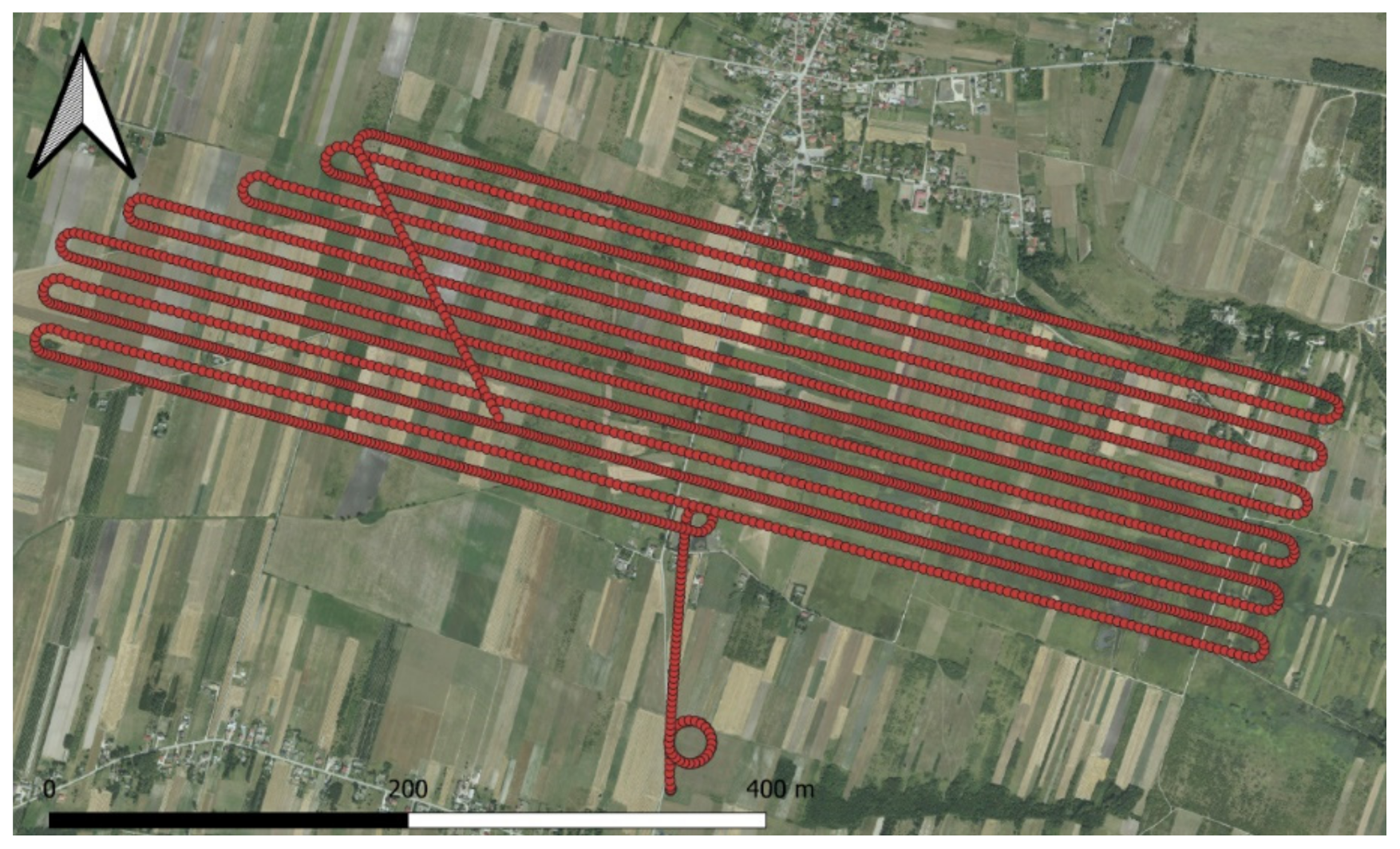
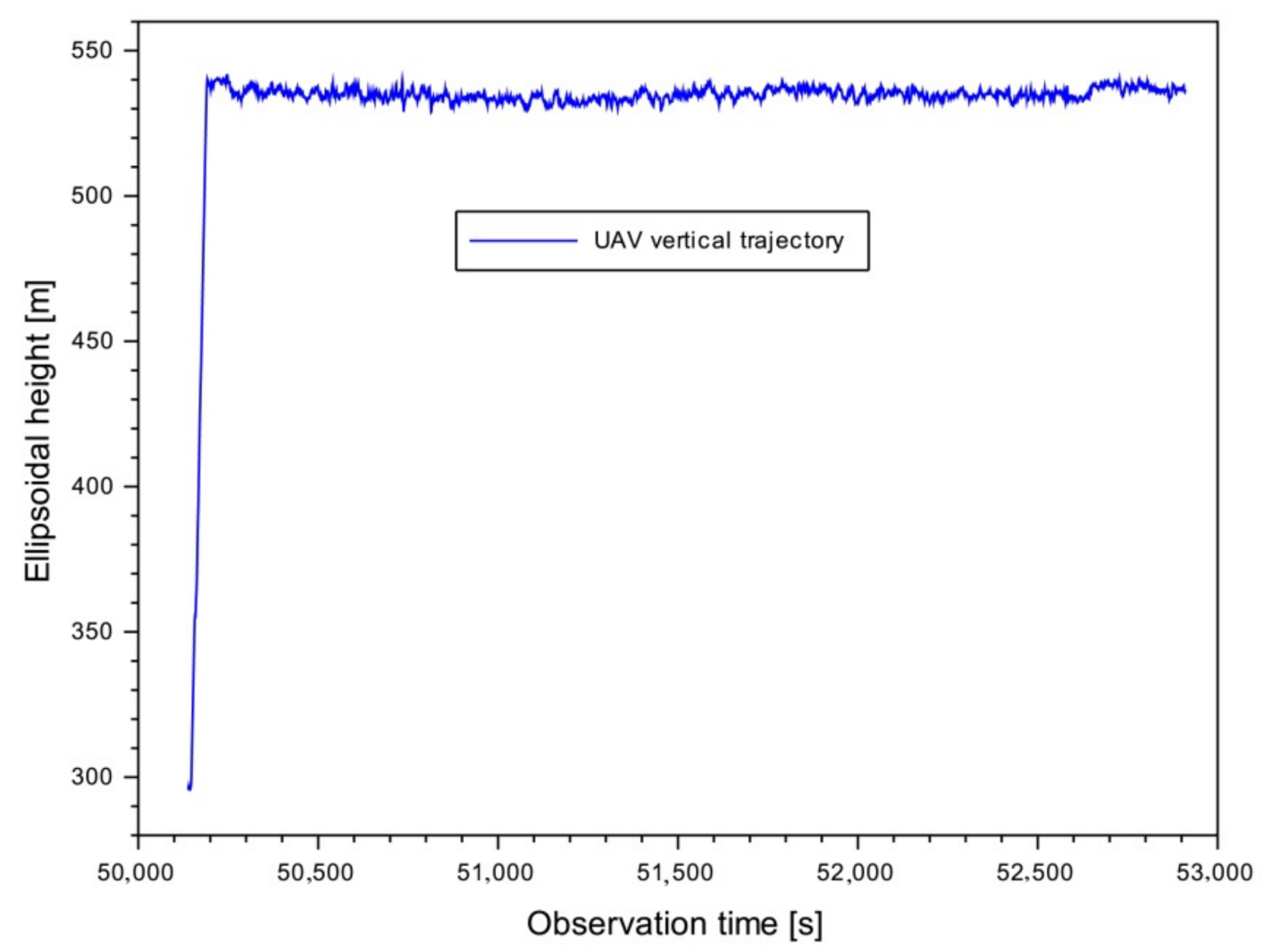
The proposed research methodology was tested and implemented into the UAV positioning model based on recorded satellite data in real-time. Satellite measurement data were collected by an AsteRx-m2 UAS receiver placed on the Tailsitter unmanned aerial vehicle [43]. The satellite observations “OBS” and the navigation message “NAV” in RINEX format were taken from the AsteRx-m2 UAS measuring device for calculations. The registration of satellite data took place on the given UAV flight route. The Tailsitter platform performed a test flight near Warsaw, Poland, in April 2020. The flight duration was from 13:55:38 to 14:41:51 GPST. The air temperature during the flight was 16 °C, and the wind speed was 6 m/s. The maximum flight speed was up to 35 m/s. Figure 2 shows a sketch of the horizontal flight trajectory, while Figure 3 shows the vertical flight trajectory of the UAV platform. The flight altitude did not exceed 250 m. The flight scenario was planned so that the land cover did not apply to the urban area. Therefore, the flight was carried out for a lowland area with mainly agricultural crops. Additionally, no tall trees or forests were found on the flight route. The flight was made in an east–west direction. In total, thirteen series of images were taken, and the side and forward overlap was 75%.

Apart from the navigation and GNSS observation data, the EGNOS and SDCM corrections in the “EMS” format were used for the calculations. The EGNOS and SDCM patches were downloaded from the website: ftp://serenad-public.cnes.fr/SERENAD0 (accessed on 10 March 2021) [44]. The first stage of the computational process concerned the preparation of the research material and its time synchronization for a 1 s interval. The input data prepared in this way were imported in the next step into the RTKPOST program [45] to determine the UAV position from a single SBAS solution, EGNOS or SDCM, respectively. At this stage, the configuration of the calculations was determined based on the parameters and models included in publications [7,46,47]. The calculated UAV coordinates from a single EGNOS and SDCM solution are expressed in ellipsoidal BLh coordinates. In a single UAV position solution using EGNOS and SDCM data, the least-squares method is used in a stochastic process. In the next step, RTKPOST reports are imported to Scilab [48] in order to calculate the resultant UAV flight position according to Algorithms (1)–(11). All the source code for the mathematical models (1)–(11) has been written in Scilab to determine the best configuration for the resultant EGNOS+SDCM position model. It is worth mentioning that the calculations used real measurement data, so determining the optimal solution strategy for the resultant EGNOS+SDCM position model for UAVs is extremely interesting for air navigation.

Additionally, the Scilab source code describes the expression for the proposed EGNOS+SDCM solution’s accuracy, according to Algorithm (12). The UAV flight reference position was determined using the RTK positioning method [37] and the RTKPOST software. All algorithms (1)–(12) implemented in Scilab allow for a detailed analysis of the selection of the optimal weighing variant for the EGNOS+SDCM positioning model for UAVs.

5. Results

Section 5 shows the research results obtained for the proposed calculation algorithms (1)–(12). First, the measuring weights were determined following Formulas (2), (5) and (7). Figure 4 shows the measurement weights as a function of the reciprocal of the number of satellites tracked from the EGNOS and SDCM solutions. In this case, the measuring weights are from 0.111 to 0.143 for the EGNOS solution and 0.111 to 0.250 for the SDCM solution, respectively. It is worth noting that the measuring scales from the EGNOS solution show a smaller dispersion than from the SDCM solution. It can be presumed that in the SDCM solution, the number of satellites for which SDCM corrections were determined was variable during the duration of the UAV flight. That is valuable technical information for the very operation of the SDCM system in air navigation.

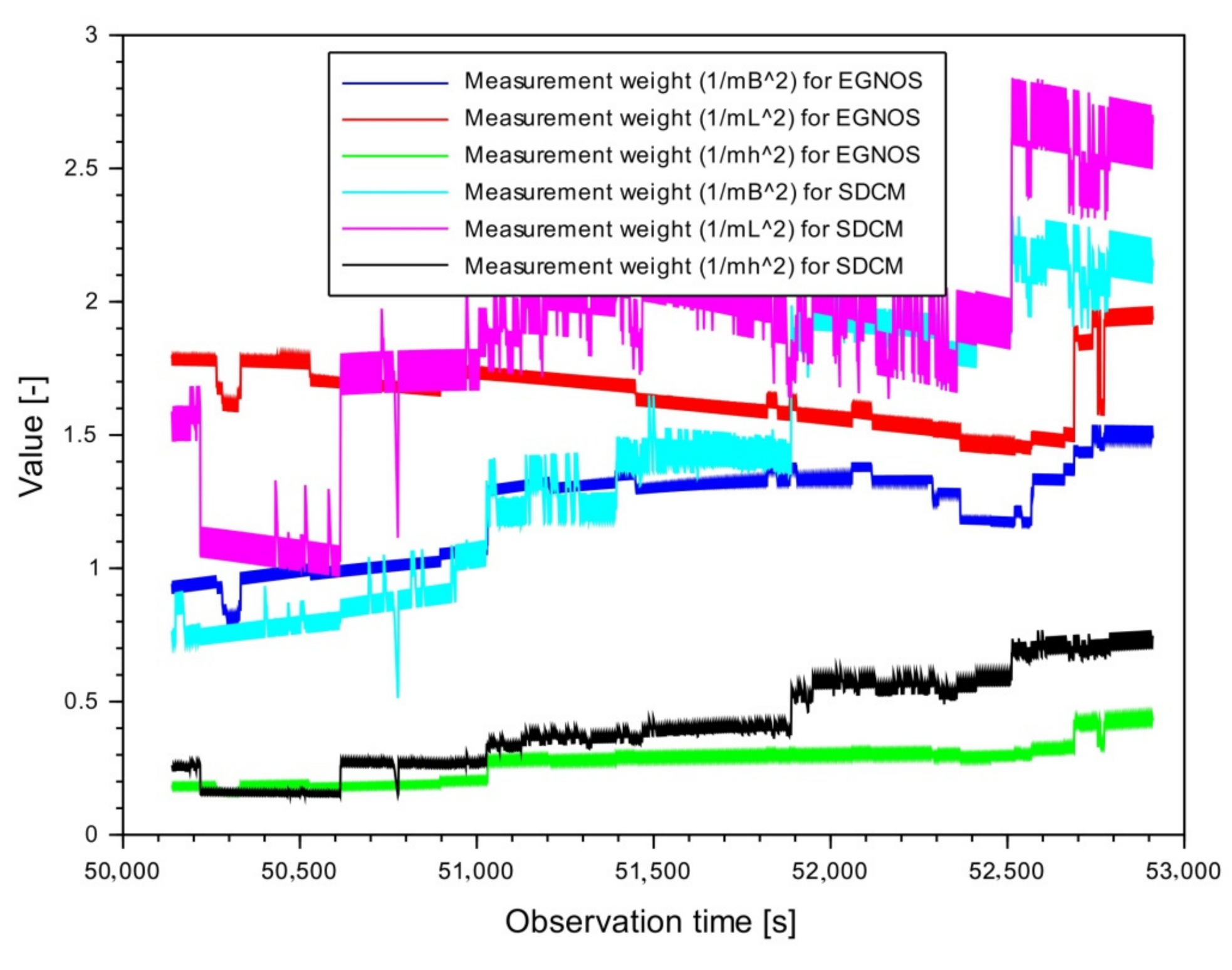
Figure 5 shows the results of measurement weights determined as a function of the inverse of the square of the mean error for the ellipsoidal coordinates BLh, separately for the EGNOS and SDCM solution. It is worth noting that the measurement weights for the horizontal components B and L are more significant than the measurement weights for the h component. In the measurement weights for the horizontal components B and L, their values range from 0.513 to 2.839 for the EGNOS and SDCM solutions, respectively. The measurement weights for the vertical component are from 0.153 to 0.768 for the EGNOS and SDCM solution. A fairly significant difference in measurement weights for the horizontal components B and L and the vertical component h depends mainly on the mean error values for the determined BLh coordinates from a single SBAS solution. It follows that the higher the mean coordinate error value, the smaller the weighing scale and vice versa.

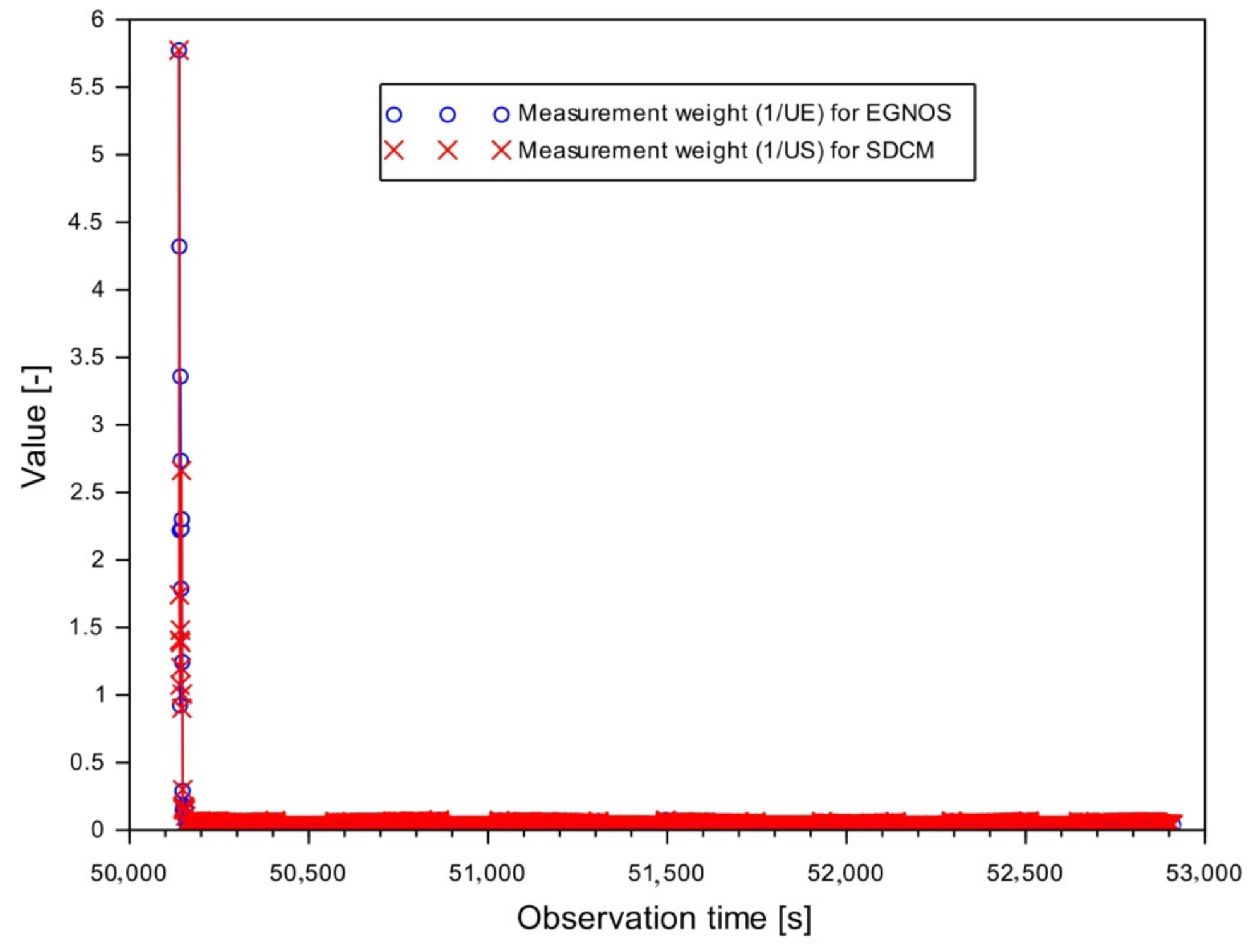
Figure 6 presents the results of measurement weights as a function of the reciprocal of the total flight speed of the UAV, separately for the EGNOS and SDCM solutions. The measurement weight values from the EGNOS and SDCM solution are from 0.029 to 5.774. At this point, one crucial element should be noted for determining the measurement weights from the Algorithms (6) and (7). Analysing the results in Figure 6, it can be seen that the values of the measurement weights differ significantly from the rest for the first ten measurement epochs. For the rest of the measurement epochs, the measurement weights are less than 0.200. However, it is essential why there is such a sharp jump in the measuring scales in the initial phase of flight. It is due to the low flight speed, below 5 m/s for both EGNOS and SDCM. For the remaining measurement epochs, this resultant flight speed changes from 15 to 35 m/s. Therefore, the difference is visible here and quite significant from the point of view of determining the navigation parameters of the UAV flight. This speed difference is typical in the UAV flight control process. During take-off, the flight speed is low; as the flight time goes on, the speed increases.

Table 2. The residuals along the B axis.

Accuracy Parameter	Measurement Weight	Value (m)
$V_B=B_E-Bm$	$\frac{1}{N{s}_i}$	Between −0.757 to 0.316
$V_B=B_E-Bm$	$\frac{1}{C{l}^2{}_i}$	Between −0.632 to 0.308
$V_B=B_E-Bm$	$\frac{1}{U_i}$	Between −0.707 to 0.296
$V_B=B_S-Bm$	$\frac{1}{N{s}_i}$	Between −0.276 to 0.541
$V_B=B_S-Bm$	$\frac{1}{C{l}^2{}_i}$	Between −0.291 to 0.726
$V_B=B_S-Bm$	$\frac{1}{U_i}$	Between −0.296 to 0.702

,

Table 3. The residuals along the L axis.

Accuracy Parameter	Measurement Weight	Value (m)
$V_L=L_E-Lm$	$\frac{1}{N{s}_i}$	Between −0.417 to 0.514
$V_L=L_E-Lm$	$\frac{1}{C{l}^2{}_i}$	Between −0.328 to 0.559
$V_L=L_E-Lm$	$\frac{1}{U_i}$	Between −0.326 to 0.509
$V_L=L_S-Lm$	$\frac{1}{N{s}_i}$	Between −0.514 to 0.275
$V_L=L_S-Lm$	$\frac{1}{C{l}^2{}_i}$	Between −0.469 to 0.408
$V_L=L_S-Lm$	$\frac{1}{U_i}$	Between −0.519 to 0.323

and

Table 4. The residuals along the h axis.

Accuracy Parameter	Measurement Weight	Value (m)
$V_h=h_E-hm$	$\frac{1}{N{s}_i}$	Between −1.244 to 1.668
$V_h=h_E-hm$	$\frac{1}{C{l}^2{}_i}$	Between −0.902 to 2.030
$V_h=h_E-hm$	$\frac{1}{U_i}$	Between −0.975 to 1.652
$V_h=h_S-hm$	$\frac{1}{N{s}_i}$	Between −1.668 to 0.711
$V_h=h_S-hm$	$\frac{1}{C{l}^2{}_i}$	Between −1.305 to 1.054
$V_h=h_S-hm$	$\frac{1}{U_i}$	Between −1.683 to 0.980

show the values of corrections for the BLh coordinates as a function of the weighting variant specified (see Algorithms (1)–(11)). The corrections were calculated according to the Formula (8). The values of corrections along the B axis are from −0.757 m to +0.726 m. The reduction of corrections is quite important from the point of view of determining the mean error $\delta B$ and the mean error of the arithmetic mean $MB$. Table 3 shows the distribution of corrections for the L component. The spread of corrections along the L axis ranges from −0.519 to +0.559 m. The results of coordinates from EGNOS and SDCM solutions to determine the resultant position of the UAV are better for the L coordinate than for the B component. Table 4 shows the correction results for the vertical h component. In this case, the scattering results are the worst, i.e., compared to the corrections for the horizontal components, there is quite a visible deterioration of the results. That is obvious since the flight ellipsoidal height was determined with the greatest errors in the mean coordinates. The dispersion of corrections along the h axis ranges from −1.683 to +2.030 m.

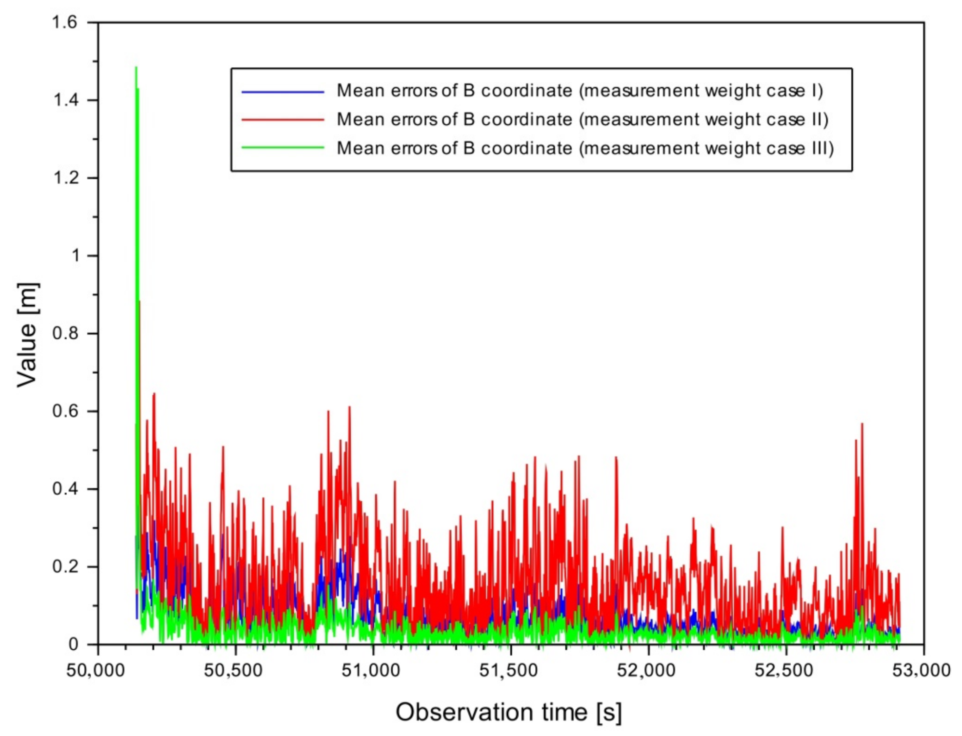
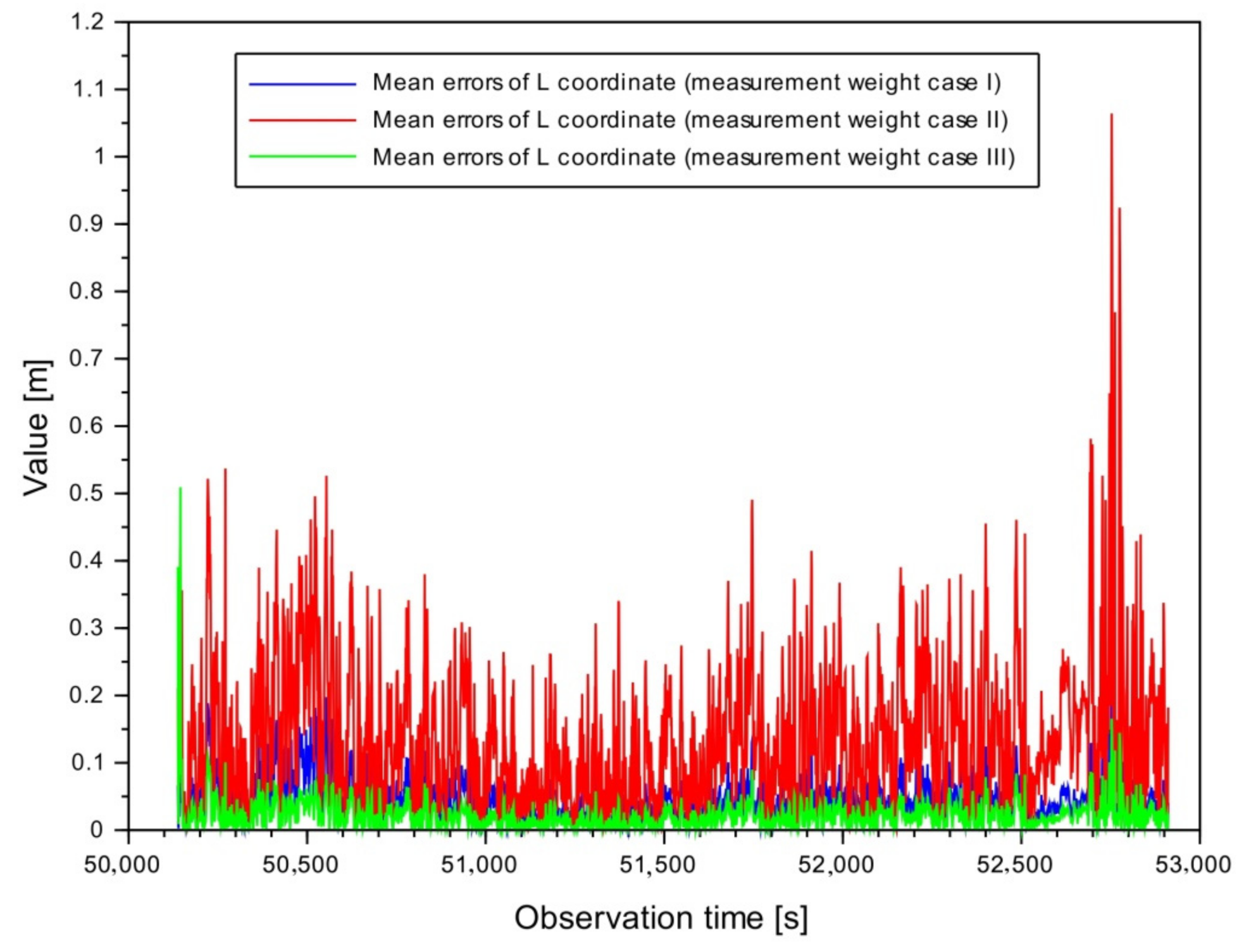
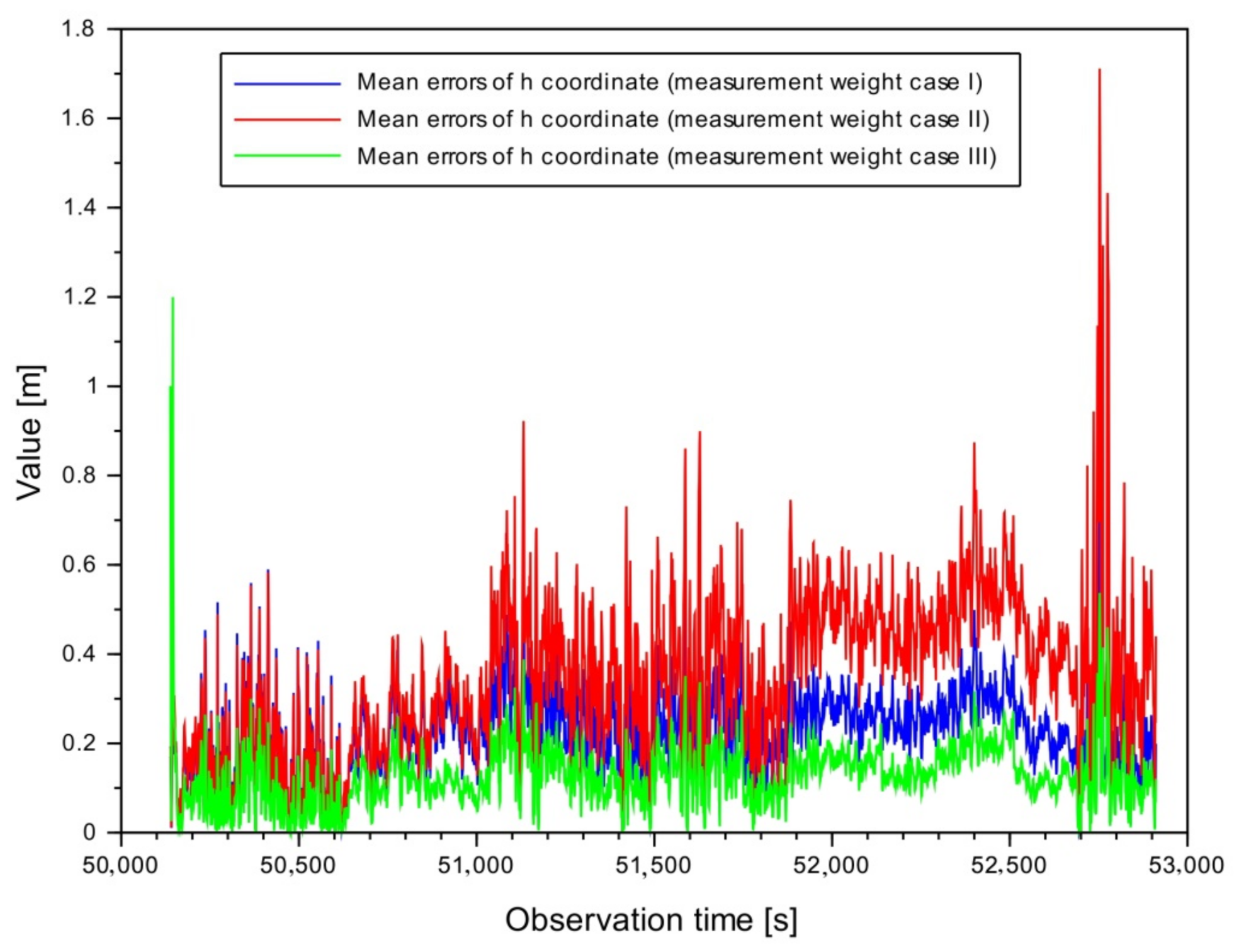
Determining the corrections following Algorithm (8) is the basis for calculating the mean errors of the resultant UAV position based on Formula (9). Figure 7, Figure 8 and Figure 9 show the results of the mean errors for the resultant UAV position. The maximum values of the parameters $\delta B$ are as follows: 0.416 m for a measuring balance Variant I, 0.885 m for a measuring balance Variant II, and 1.487 m for a measuring balance Variant III. The average value of the $\delta B$ parameter is, in turn, 0.061 m for a measuring balance, Variant I, 0.155 m for a measuring balance, Variant II, and 0.033 m for a measuring balance, Variant III. The maximum values of the $\delta L$ parameters are as follows: 0.242 m for a measuring balance Variant I, 1.064 m for a measuring balance Variant II, and 0.509 m for a measuring balance Variant III. On the other hand, the average value of the $\delta L$ parameter is equal to 0.039 m for a measuring balance, Variant I, 0.136 m for a measuring balance, Variant II, and 0.022 m for a measuring balance, Variant III. The maximum values of the parameters $\delta h$ are, respectively, 0.786 m for a measuring balance Variant I, 1.711 m for a measuring balance Variant II, 1.199 m for a measuring balance Variant III. On the other hand, the average value of the parameter $\delta h$ is equal to 0.221 m for a measuring balance, Variant I, 0.343 m for a measuring balance, Variant II, and 0.128 m for a measuring balance, Variant III. When analysing the results of the parameters $\left(\delta B,\delta L,\delta h\right)$, it can be noticed that the best results of the mean errors are visible for the weighing scale Variant III. Of course, there are single outliers of $\delta B$, as shown in Figure 7. However, objectively, the best results were obtained for the weighing as a function of the reciprocal of the airspeed.

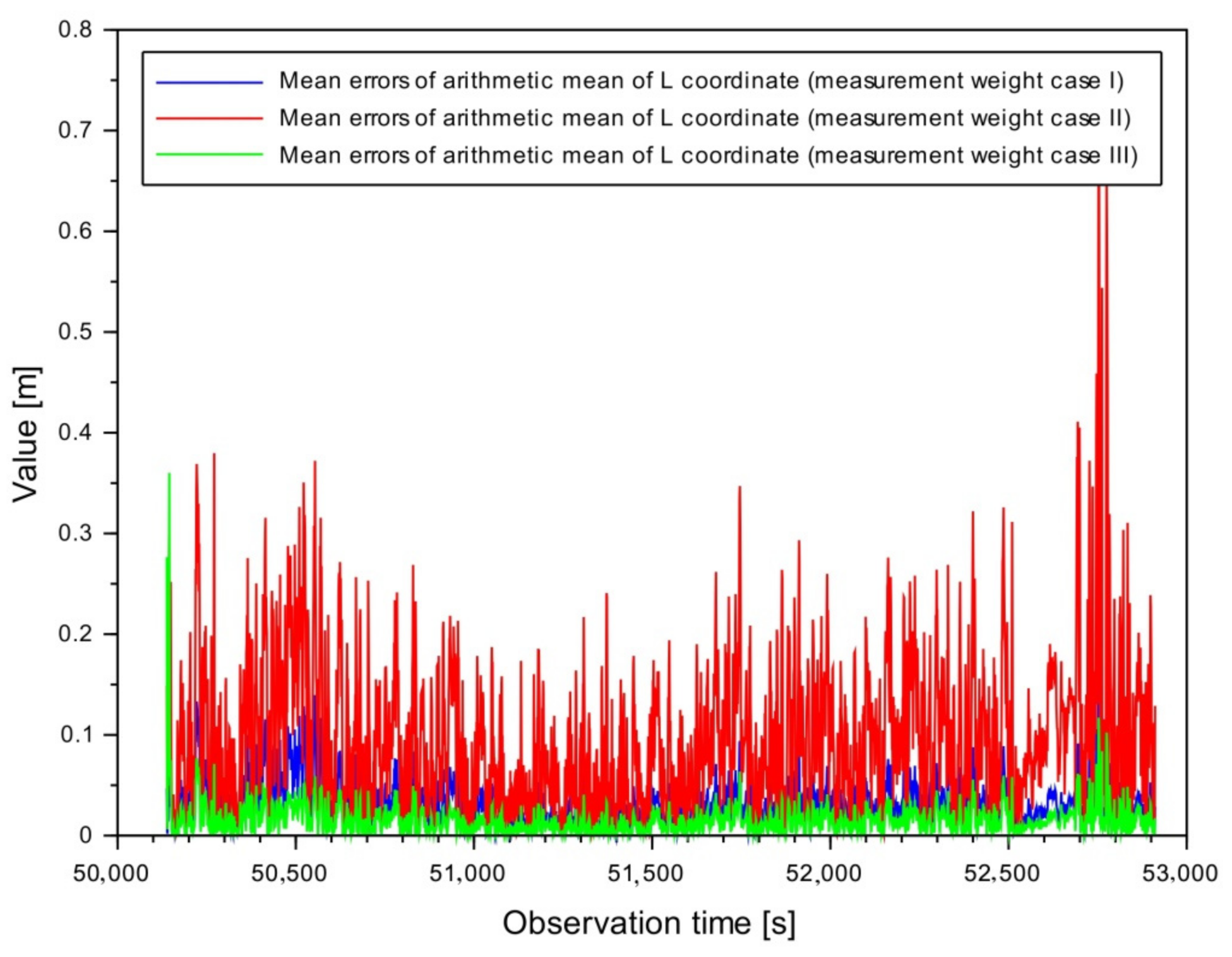
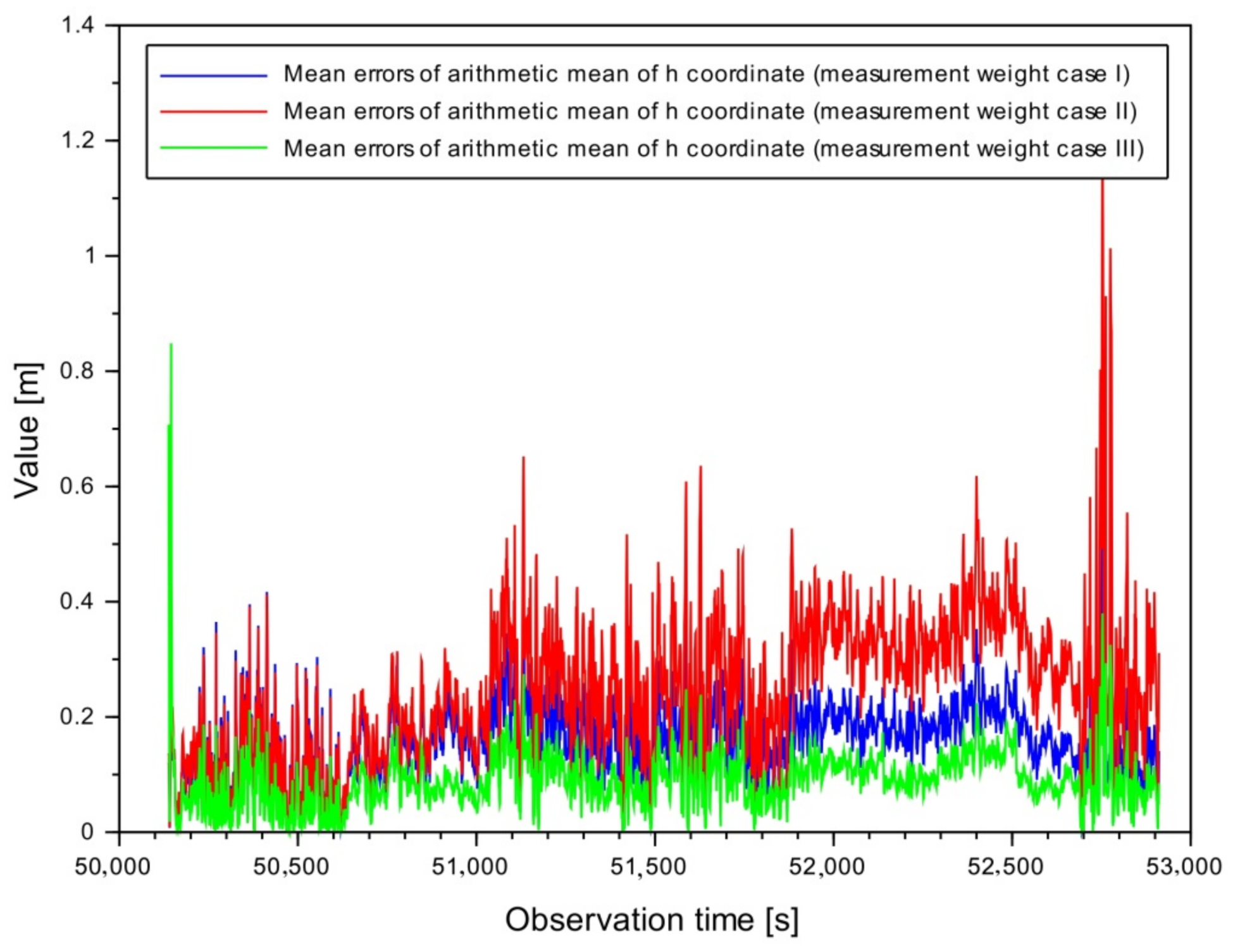
Figure 10, Figure 11 and Figure 12 present the research results on the determination of the mean errors of the arithmetic mean for the resultant UAV position on the basis of the common EGNOS+SDCM solution. The parameter values $\left(MB,ML,Mh\right)$ were determined by the mathematical Equation (10). The average value of the $MB$ parameter is 0.043 m for a measuring balance, Variant I, 0.109 m for a measuring balance, Variant II, and 0.023 m for a measuring balance, Variant III. On the other hand, the average value of the $ML$ parameter is equal to 0.028 m for a measuring balance, Variant I, 0.096 m for a measuring balance, Variant II, and 0.016 m for a measuring balance, Variant III. Moreover, the average value of the $Mh$ parameter achieves the following results: 0.156 m for a measuring balance, Variant I, 0.243 m for a measuring balance, Variant II, and 0.090 m for a measuring balance, Variant III. Similar to the analysis of the $\left(\delta B,\delta L,\delta h\right)$ parameter results, the results of mean errors of the arithmetic mean $\left(MB,ML,Mh\right)$ are the best for weighing in Variant III.

In

Table 5. The results of the global Chi-square test.

Coordinate	Measurement Weight	Maximum Values of $\sum {\mathit{V}}_{\mathit{B}}^{\mathit{T}}\mathit{·}{\mathit{w}}_{\mathit{i}}\mathit{·}{\mathit{V}}_{\mathit{B}}$	Statistical Value of ${\mathit{\varkappa }}_{\mathit{f},\mathit{k}}^2$
B	$\frac{1}{N{s}_i}$	0.416	3.841
B	$\frac{1}{C{l}^2{}_i}$	0.885	3.841
B	$\frac{1}{U_i}$	1.487	3.841
Coordinate	Measurement weight	Maximum values of$\sum V_L^T·w_i·V_L$	Statistical value of${\varkappa }_{f,k}^2$
L	$\frac{1}{N{s}_i}$	0.242	3.841
L	$\frac{1}{C{l}^2{}_i}$	1.064	3.841
L	$\frac{1}{U_i}$	0.509	3.841
Coordinate	Measurement weight	Maximum values of$\sum V_h^T·w_i·V_h$	Statistical value of${\varkappa }_{f,k}^2$
h	$\frac{1}{N{s}_i}$	0.787	3.841
h	$\frac{1}{C{l}^2{}_i}$	1.711	3.841
h	$\frac{1}{U_i}$	1.199	3.841

, a statistical analysis was performed for the obtained test results based on Equation (11). For this purpose, the global Chi-square test was performed at the confidence level $k=1-\alpha$ for the $f=n-1$ number of degrees of freedom. In the analysed experiment, the significance level is equal to $\alpha =0.05$, and the confidence level: $1-\alpha =0.95$ [42]. Moreover, the number of degrees of freedom is $f=n-1=2-1=1$. For the obtained results of the resultant BLh coordinates and for all measurement weights, the sum of the mathematical expressions $\sum V_B^T·w_i·V_B$, $\sum V_L^T·w_i·V_L,$ and $\sum V_h^T·w_i·V_h$ is lower than the tabular value of the Chi-square test ${\varkappa }_{f,k}^2$. It can therefore be said that the global Chi-square test ${\varkappa }_{f,k}^2$ has been met. Moreover, the proposed calculation algorithms (1)–(11) are correct for a given confidence level and a given number of degrees of freedom. Finally, the internal reliability test was checked, and it turned out to be correct for the research experiment performed.

6. Discussion

When determining the suitability of a given research method, the critical element is to determine the accuracy of the presented solution. In the presented work, the accuracy of the presented solution was determined following Equation (12). On this basis, the results of the resultant UAV position concerning the flight reference trajectory, calculated by the RTK differential technique, were compared. The determination of position errors $\left(dB,dL,dh\right)$ allows determining which weighting strategy is the best for calculating the resultant position of the UAV from the common EGNOS+SDCM solution. That is the essential element in the context of developing the navigation results of the UAV positions.

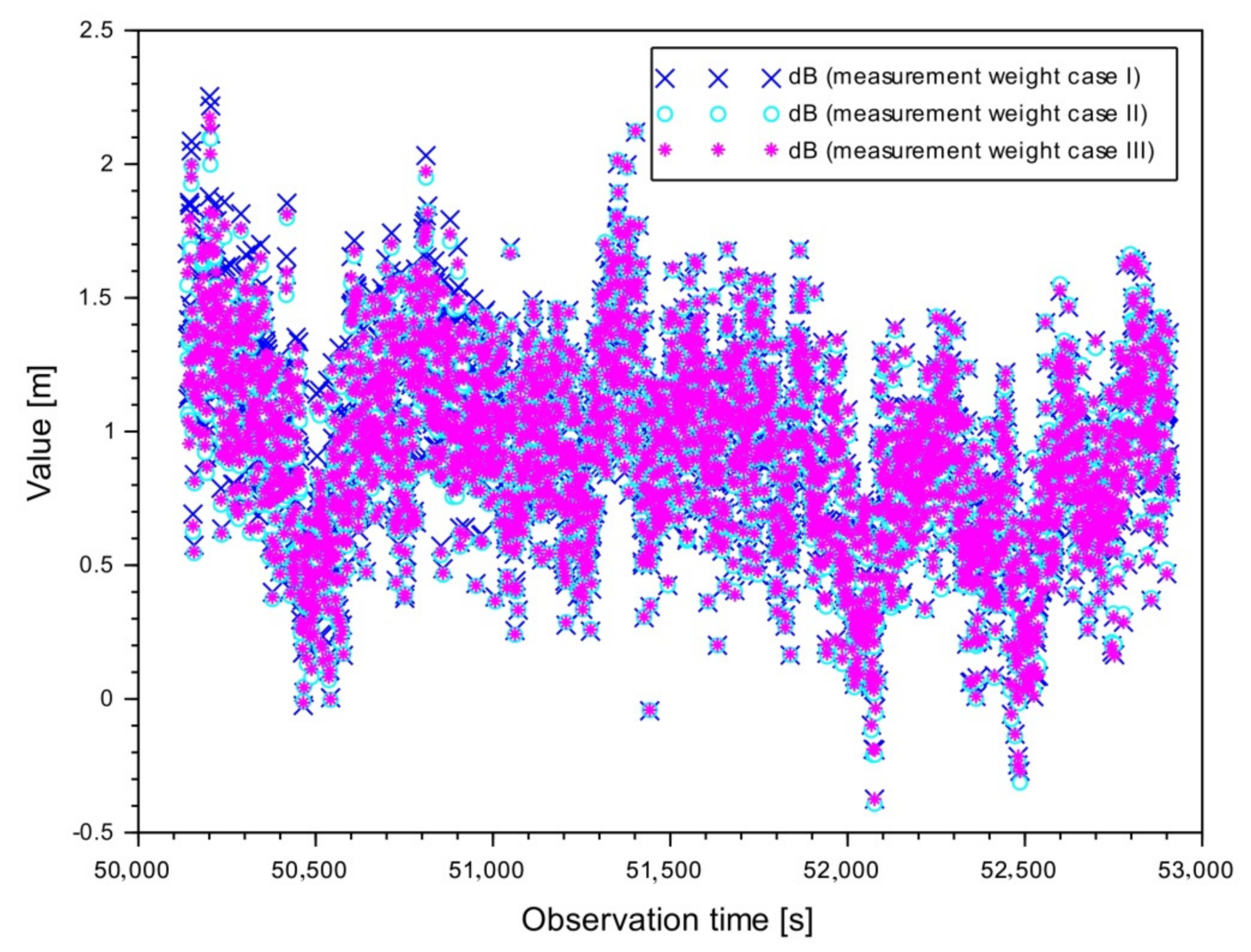
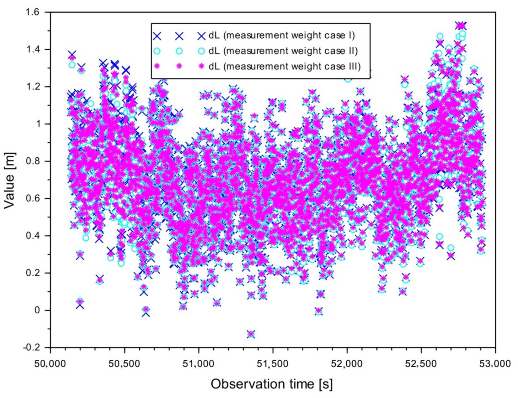
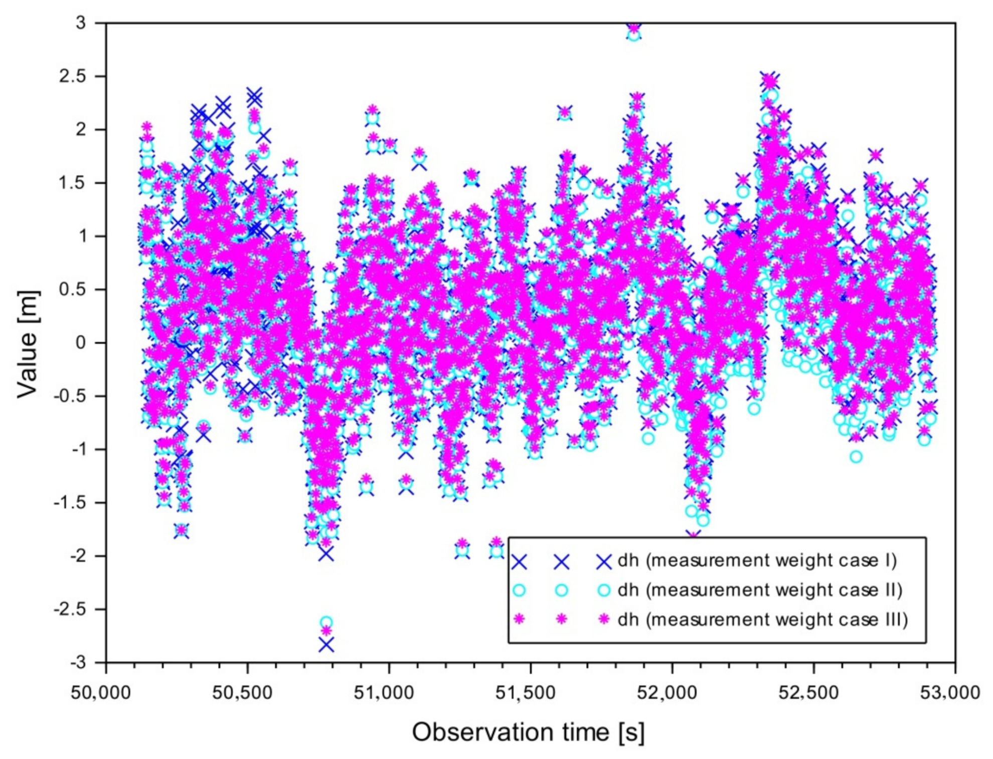
In Figure 13, Figure 14 and Figure 15, the position errors $\left(dB,dL,dh\right)$ have been identified and determined. The position error values $dB$ are, respectively, from −0.375 to +2.252 m for the weighing Variant I, from −0.392 to +2.123 m for the weighing Variant II, and from −0.375 to +2.174 m for the weighing Variant III. In turn, the position errors $dL$ are from −0.129 to +1.528 m for the weighing Variant I, from −0.128 to +1.485 m for the weighing Variant II, and from −0.127 to +1.531 m for the weighing Variant III. Moreover, the position errors $dh$ achieved the following results: from −2830 to +2922 m for the weighing Variant I, from −2623 to +2888 m for the weighing Variant II, and from −2699 to +2950 m for the weighing Variant III.

In addition, as part of the accuracy analysis, the average positioning accuracy was determined according to the relationship:

$$\left\{\begin{array}{c}\overline{dB}=\frac{\sum dB}{N}\\ d\overline{L}=\frac{\sum dL}{N}\\ \overline{dh}=\frac{\sum dh}{N}\end{array}\right.$$

(13)

where:

$\left(\overline{dB},\overline{dL},\overline{dh}\right)$—average accuracy, arithmetic mean of position errors $\left(dB,dL,dh\right)$,

$N$—number of measurement epochs, number of independent UAV position readings from the EGNOS+SDCM joint solution.

Based on the performed calculations, it was found that the $\overline{dB}$ parameter values are 0.934 m for the weighing Variant I, 0.919 m for the weighing Variant II, and 0.924 m for the weighing Variant III. In turn, the $\overline{dL}$ values are equal, respectively, 0.712 m for the weighing Variant I, 0.706 m for the weighing Variant II, and 0.710 m for the weighing Variant III. On the other hand, average accuracy $\overline{dh}$ results reach the following results: 0.366 m for the weighing Variant I, 0.295 m for the weighing Variant II, and 0.381 m for the weighing Variant III.

The results calculated from Equation (13) are shown collectively in

Table 6. The summary of accuracy analysis.

Accuracy Parameter	Measurement Weight	Value (m)	Comment
$\overline{dB}$	$\frac{1}{N{s}_i}$	0.934	The highest accuracy is visible for the weighing Variant II
$\overline{dB}$	$\frac{1}{C{l}^2{}_i}$	0.919
$\overline{dB}$	$\frac{1}{U_i}$	0.924
$\overline{dL}$	$\frac{1}{N{s}_i}$	0.712	The highest accuracy is visible for the weighing Variant II
$\overline{dL}$	$\frac{1}{C{l}^2{}_i}$	0.706
$\overline{dL}$	$\frac{1}{U_i}$	0.710
$\overline{dh}$	$\frac{1}{N{s}_i}$	0.366	The highest accuracy is visible for the weighing Variant II
$\overline{dh}$	$\frac{1}{C{l}^2{}_i}$	0.295
$\overline{dh}$	$\frac{1}{U_i}$	0.381

. On the basis of results in Table 6, it can be observed that the highest accuracy was noted in Variant II. In turn, the lowest positioning accuracy is for weighting measurements as a function of the reciprocal of the number of satellites tracked. The results in Table 6 show a relatively good positioning accuracy for weighting measurements for Variant III, especially for the horizontal components B and L.

Analysing the results in Figure 13, Figure 14 and Figure 15 and using Formulas (12) and (13), it can be observed that the highest accuracy is for the weighing Variant II, i.e., measuring weight is expressed as a function of the inverse square of the mean error of the coordinates. On the other hand, the lowest positioning accuracy is visible when a weighing scale is used in calculations as a function of the reciprocal of the number of satellites. It is also worth looking at the results of the parameters $\left(\overline{dB},\overline{dL},\overline{dh}\right)$ and determining how much the UAV positioning accuracy has improved for the weighing Variant II to the results of the Variants I and III. To this end, the improvement in positioning accuracy for Variant II was determined as a percentage, as written in Equation (14) below:

$$\left\{\begin{array}{c}P{B}_{II}=\left\{\begin{array}{c}\frac{\overline{d{B}_{II}}-\overline{d{B}_I}}{\overline{d{B}_I}}·100\%\\ \frac{\overline{d{B}_{II}}-\overline{d{B}_{III}}}{\overline{d{B}_{III}}}·100\%\end{array}\right.\\ P{L}_{II}=\left\{\begin{array}{c}\frac{\overline{d{L}_{II}}-\overline{d{L}_I}}{\overline{d{L}_I}}·100\%\\ \frac{\overline{d{L}_{II}}-\overline{d{L}_{III}}}{\overline{d{L}_{III}}}·100\%\end{array}\right.\\ P{h}_{II}=\left\{\begin{array}{c}\frac{\overline{d{h}_{II}}-\overline{d{h}_I}}{\overline{d{h}_I}}·100\%\\ \frac{\overline{d{h}_{II}}-\overline{d{h}_{III}}}{\overline{d{h}_{III}}}·100\%\end{array}\right.\end{array}\right.$$

(14)

where:

$(P{B}_{II},P{L}_{II},P{L}_{II})$—the percentage expression of the improvement in positioning accuracy for component B from the weighting Variant II with respect to the results from Variants I and III;

($\overline{d{B}_I},\overline{d{L}_I},\overline{d{h}_I})$—average positioning accuracy for the weighing Variant I (see Equation (13));

($\overline{d{B}_{II}},\overline{d{L}_{II}},\overline{d{h}_{II}})$—average positioning accuracy for the weighing Variant II (see Equation (13));

($\overline{d{B}_{III}},\overline{d{L}_{III}},\overline{d{h}_{III}})$—average positioning accuracy for the weighing Variant III (see Equation (13)).

The average accuracy $\overline{d{B}_{II}}$ scores improved by 2% against the $\overline{d{B}_I}$ position error scores and 1% against the $\overline{d{B}_{III}}$ position error scores, respectively. Meanwhile, the average accuracy $\overline{d{L}_{II}}$ improved by more than 1% against the $\overline{d{L}_I}$ position error results and 1% against the $\overline{d{L}_{III}}$ position error scores, respectively. On the other hand, the $\overline{d{h}_{II}}$ average accuracy improved by over 19% to the $\overline{d{h}_I}$ position error scores and more than 22%, respectively, against the $\overline{d{h}_{III}}$ position error scores. As can be seen, a significant improvement is observed for the vertical component h. Here, the percentage results are 19 ÷ 22%. It can be seen from the results of $dh$ position errors that the differences for this component are visible, which has an impact on determining the accuracy in percentage terms, according to Formula (14). On the other hand, for the horizontal components B and L, practically, the $\left(dB,dL\right)$ position error results are the same, and hence the $(P{B}_{II},P{L}_{II})$ parameter values in percentage terms are 1 ÷ 2%. Now, analysing the results of the $(P{B}_{II},P{L}_{II}, P{h}_{II})$ parameters for individual variants, it can be said that:

-

the improvement of the accuracy of Solution II in relation to the results from Variant I is, respectively, 2% for the B component, 1% for the L component, and 19% for the h component;

-

the improvement of the accuracy of Solution II in relation to Variant III results is 1% for the B component, 1% for the L component, and 22% for the h component.

On this basis, it can be seen that the positioning accuracy results for the horizontal components B and L for Variants I, II, and III are similar. This information is essential for UAV navigation in the horizontal plane. In comparing the positioning accuracy for the vertical component h, a significant difference can be noticed in the determination of position errors from Variant II concerning the results from Variants I and III. It seems that the research results presented in the paper can be directly translated and implemented into UAV technology in terms of the implementation of GNSS satellite systems and SBAS support systems.

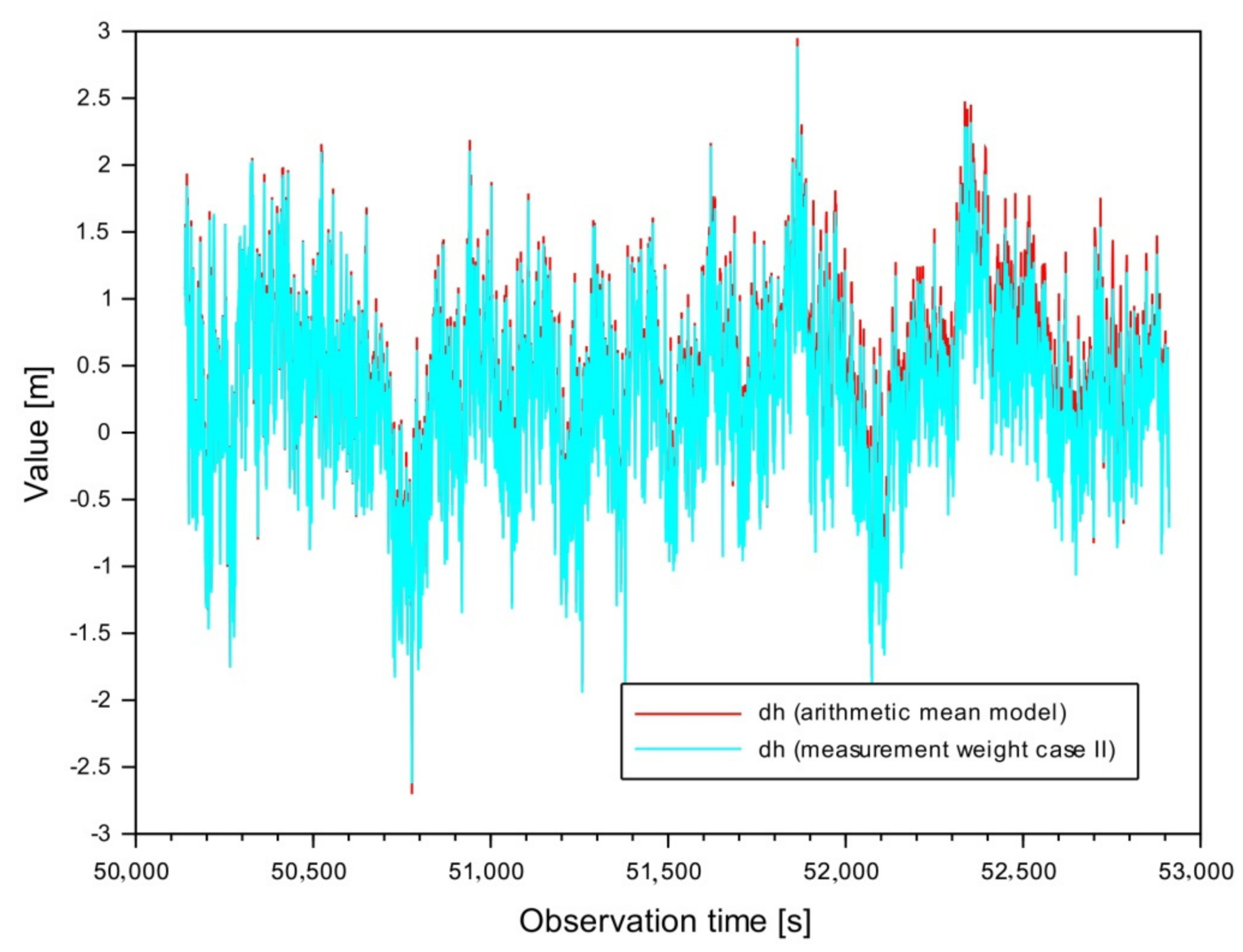
Another research problem was raised in the discussion. Namely, as the position error results show, the positioning accuracies for the horizontal components B and L are at a similar level of values. The deviation occurs only for the vertical component h. Therefore, two additional experiments were performed, in which, first, the accuracy of determining the ellipsoidal height from the weighing Variant II was compared with the arithmetic mean model, and second, the influence of the SDCM+EGNOS solution in relation to for a single EGNOS solution for the vertical component h was determined. Figure 16 shows the positioning accuracy of the UAV along the h axis for the weighting model II and based on the arithmetic mean model [7]. The positioning accuracy results for the h component from the solution of the weighted average model for Variant II are shown in Figure 15 and described in detail in the paper. In turn, the accuracy of determining the h component from the arithmetic mean model ranges from −2.703 to +2.949 m. Moreover, the average positioning accuracy for the h component from the arithmetic mean model is +0.381 m, according to Formula (13). On the other hand, using Formula (14), the percent improvement in positioning accuracy for the h component of the weighted average model (Variant II) in relation to the results from the arithmetic mean model is about 23%. It can be seen that the method of weighting is crucial for vertical flight stabilization. Using the weighting model for Variant II, a significant improvement in the positioning accuracy for the ellipsoidal height h can be noticed. The obtained test results only confirm the correctness of the appropriate selection of the weighing model.

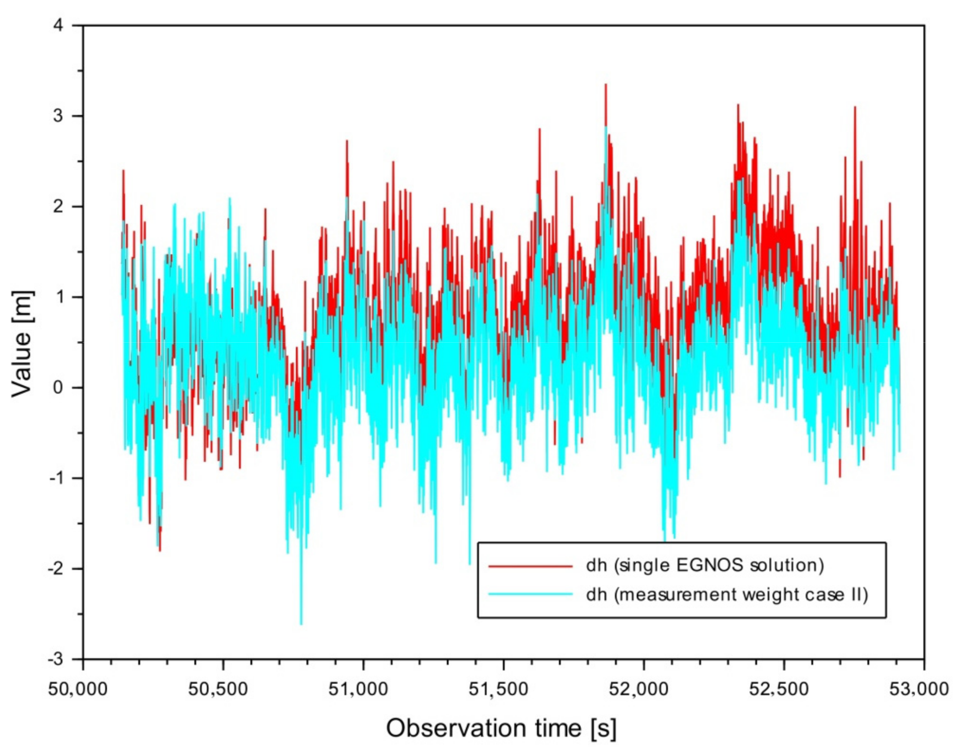
Moving on to the second stage of the analysis, Figure 17 shows the impact of the EGNOS+SDCM solution on the accuracy of the h-component determination to the results from only a single EGNOS SBAS solution. Please note how the SBAS SDCM support system significantly improved the positioning accuracy for the ellipsoidal height h. In the case of a single EGNOS solution, we speak of position errors from −1.941 to +3.357 m. The average positioning accuracy along the h axis of the EGNOS solution is 0.735 m. On this basis, it can be concluded that the weight model for Variant II improved the positioning accuracy of the ellipsoidal height h by approximately 60% compared to the results from a single EGNOS solution. That is a key issue as it shows that SDCM can provide a great added value to the EGNOS booster system, which has already been tested many times. All the more, scientific research should become directional in search of increasingly better solutions for navigating UAV positions for vertical flight stabilization. If subsequent studies would confirm the effectiveness of applying the SDCM system in UAV technology, it would be an important alternative to the EGNOS system, especially in Europe.

It seems that the developed algorithm and the obtained test results show one regularity, i.e., they show new navigation solutions for improving the performance of determining UAV coordinates and, above all, improving the accuracy of UAV positioning. A similar procedure of the solution was used in most scientific works [12,13,14,15,16,17,18,19,20,21,22,23,24,25,26,27,28,29,30,31,32,33,34], where new navigation possibilities were searched for to improve the precise positioning of the UAV. UAV position navigation solutions in the works [12,13,14,15,16,17,18,19,20,21,22,23,24,25,26,27,28,29,30,31,32,33,34] concerned either a single SBAS solution or a multi-SBAS solution directly. This shows a great need to develop modern GNSS navigation algorithms in UAV technology in many research planes. The positioning algorithm for the mathematical Equations (1)–(11) presented in the paper fits perfectly into this research trend.

7. Conclusions

This article presents a new solution for navigating UAV positions with the use of SBAS assistance systems. Namely, the article presents a new UAV positioning algorithm based on the fusion of multi-SBAS positioning in air navigation. In air navigation, newer and better mathematical algorithms are being sought to improve UAV positioning. Hence, the paper proposes using a linear combination of single SBAS position navigation solutions to improve the determination of the resultant UAV coordinates. The linear combination was based on the weighted average model, which used a weighting scheme for three variants: Variant I, the inverse of the number of satellites tracked from a single SBAS solution; Variant II, the inverse square of the mean coordinate errors from a single SBAS solution; and Variant III, the reciprocal of the UAV flight speed from a single SBAS solution.

For these three schemas, an advanced mathematical algorithm was developed and used in numerical calculations in Scilab. The actual GNSS navigation data recorded by the Tailsitter unmanned platform were used in the calculations. The test flight was made in April 2020 in Poland, near Warsaw. In addition, SBAS corrections and the RTKPOST application were used in the calculations. Based on the developed research results, it was found that the highest accuracy of UAV positioning was obtained when using the weighting model for Variant II. In the weighting model of Variant II, the accuracy of the solution of the UAV position increased by 1–2% for the horizontal components and 19–22% for the vertical component h, concerning the results obtained from the weighting Variants I and III. It is worth noting that the proposed research model significantly improves the results of determining the ellipsoidal height h. Compared to the arithmetic mean model, the accuracy of the determination of the h component in the weight model Variant II is improved by about 23%. The paper also shows the advantage of EGNOS+SDCM positioning to the EGNOS positioning itself in determining the accuracy of the vertical component h. The obtained research results show the significant advantages of the multi-SBAS positioning model in UAV technology.

In the future, it is planned to perform further research tests in which the problem of testing the accuracy of UAV positioning with the use of SBAS assist systems will be discussed. In particular, further research is planned for the EGNOS and SDCM augmentation systems. The conducted research work can be used to improve the position of the UAV for typically photogrammetric studies [49].

References

- EASA. Concept of Operations for Drones. 2015, p. 12. Available online: https://www.easa.europa.eu/sites/default/files/dfu/204696_EASA_concept_drone_brochure_web.pdf (accessed on 10 March 2021).
- Wierzbicki, D.; Krasuski, K. Determination the coordinates of the projection center in the digital aerial triangulation using data from Unmanned Aerial Vehicle. Aparatura Badawcza i Dydaktyczna 2016, 3, 127–134. (In Polish) [Google Scholar]
- Wierzbicki, D.; Krasuski, K. Determining the Elements of Exterior Orientation in Aerial Triangulation Processing Using UAV Technology. Commun. Sci. Lett. Univ. Zilina 2020, 22, 15–24. [Google Scholar] [CrossRef]
- Lalak, M.; Wierzbicki, D.; Kędzierski, M. Methodology of Processing Single-Strip Blocks of Imagery with Reduction and Optimization Number of Ground Control Points in UAV Photogrammetry. Remote Sens. 2020, 12, 3336. [Google Scholar] [CrossRef]
- Jimenez-Baňos, D.; Powe, M.; Raj Matur, A.; Toran, F.; Flament, D.; Chatre, E. EGNOS Open Service guidelines for receiver manufacturers. In Proceedings of the 24th International Technical Meeting of the Satellite Division of the Institute of Navigation (ION GNSS 2011), Portland, OR, USA, 19–23 September 2011; pp. 2505–2512. [Google Scholar]
- Krasuski, K.; Wierzbicki, D. Monitoring Aircraft Position Using EGNOS Data for the SBAS APV Approach to the Landing Procedure. Sensors 2020, 20, 1945. [Google Scholar] [CrossRef] [PubMed] [Green Version]
- Krasuski, K.; Wierzbicki, D. Application the SBAS/EGNOS Corrections in UAV Positioning. Energies 2021, 14, 739. [Google Scholar] [CrossRef]
- Ciećko, A.; Grunwald, G. Klobuchar, NeQuick G, and EGNOS Ionospheric Models for GPS/EGNOS Single-Frequency Positioning under 6–12 September 2017 Space Weather Events. Appl. Sci. 2020, 10, 1553. [Google Scholar] [CrossRef] [Green Version]
- Yang, L.; Wang, J.; Li, H.; Balz, T. Global Assessment of the GNSS Single Point Positioning Biases Produced by the Residual Tropospheric Delay. Remote Sens. 2021, 13, 1202. [Google Scholar] [CrossRef]
- Sanz Subirana, J.; Juan Zornoza, J.M.; Hernandez-Pajares, M. Fundamentals and algorithms. In GNSS Data Processing; ESA Communications ESTEC: Noordwijk, The Netherlands, 2013; Volume 1, ISBN 978-92-9221-886-7. [Google Scholar]
- Grzegorzewski, M.; Ciecko, A.; Oszczak, S.; Popielarczyk, D. Autonomous and EGNOS Positioning Accuracy Determination of Cessna Aircraft on the Edge of EGNOS Coverage. In Proceedings of the 2008 National Technical Meeting of The Institute of Navigation, San Diego, CA, USA, 28–30 January 2008; pp. 407–410. [Google Scholar]
- Balsi, M.; Prem, S.; Williame, K.; Teboul, D.; Délétraz, L.; Hebrard Capdeville, P.I. Establishing new foundations for the use of remotely-piloted aircraft systems for civilian applications. Int. Arch. Photogramm. Remote Sens. Spatial Inf. Sci. 2019, 2, 197–201. [Google Scholar] [CrossRef] [Green Version]
- Yoon, H.; Seok, H.; Lim, C.; Park, B. An Online SBAS Service to Improve Drone Navigation Performance in High-Elevation Masked Areas. Sensors 2020, 20, 3047. [Google Scholar] [CrossRef]
- Sheridan, I. Drones and global navigation satellite systems: Current evidence from polar scientists. R. Soc. Open Sci. 2020, 7, 191494. [Google Scholar] [CrossRef] [Green Version]
- Alarcón, F.; Viguria, A.; Vilardaga, S.; Montolio, J.; Soley, S. EGNOS-based Navigation and Surveillance System to Support the Approval of RPAS Operations. In Proceedings of the 9th SESAR Innovation Days, Athens, Greece, 2–6 December 2019. [Google Scholar]
- Tamouridou, A.A.; Alexandridis, T.; Pantazi, X.; Lagopodi, A.L.; Kashefi, J.; Kasampalis, D.A.; Kontouris, G.; Moshou, D. Application of Multilayer Perceptron with Automatic Relevance Determination on Weed Mapping Using UAV Multispectral Imagery. Sensors 2017, 17, 2307. [Google Scholar] [CrossRef]
- Molina, P.; Colomina, I.; Vitoria, T.; Silva, P.F.; Stebler, Y.; Skaloud, J.; Kornus, W.; Prades, R. EGNOS-based multi-sensor accurate and reliable navigation. ISPRS Int. Arch. Photogramm. Remote. Sens. Spat. Inf. Sci. 2012, 1, 87–93. [Google Scholar] [CrossRef] [Green Version]
- Molina, P.; Colomina, I.; Vitoria, T.; Freire, P.; Skaloud, J.; Kornus, W.; Mata, R.; Aguilera, C. The CLOSE-SEARCH project UAV-based search operations using thermal imaging and EGNOS-SoL navigation. In Proceedings of the GeoInformation for Disaster Management Conference (Gi4DM 2011), Antalya, Turkey, 3–7 May 2011. [Google Scholar]
- Molina, P.; Colomina, I.; Victoria, T.; Skaloud, J.; Kornus, W.; Prades, R.; Aguilera, C. Searching lost people with UAVS: The system and results of the CLOSE-SEARCH project. Int. Arch. Photogramm. Remote Sens. Spat. Inf. Sci. 2012, 39, 441–446. [Google Scholar] [CrossRef] [Green Version]
- Molina, P.; Colomina, I.; Vitoria, T.; Silva, P.F.; Bandeiras, J.; Stebler, Y.; Skaloud, J.; Kornus, W.; Prades, R.; Aguilera, C. Integrity Aspects of Hybrid EGNOS-based Navigation on Support of Search-And-Rescue Missions with UAVs. In Proceedings of the 24th International Technical Meeting of the Satellite Division of The Institute of Navigation (ION GNSS 2011), Portland, OR, USA, 20–23 September 2011; pp. 3773–3781. [Google Scholar]
- Fellner, A.; Sulkowski, J.; Trominski, P.; Zadrag, P. The use of reference systems for UAV flight routing. In Proceedings of the EGU General Assembly, Vienna, Austria, 22–27 April 2012; p. 6434. [Google Scholar]
- Pullen, S.; Enge, P.; Lee, J. Local-Area Differential GNSS Architectures Optimized to Support Unmanned Aerial Vehicles (UAVs). In Proceedings of the International Technical Meeting of the Institute of Navigation (ION ITM 2013), San Diego, CA, USA, 28–30 January 2013; pp. 559–571. [Google Scholar]
- Watanabe, Y.; Manecy, A.; Hiba, A.; Nagai, S.; Shin, A. Vision-integrated navigation system for aircraft final approach in case of GNSS/SBAS or ILS failures. In Proceedings of the AIAA Scitech 2019, San Diego, CA, USA, 7–11 January 2009; p. 113. [Google Scholar]
- Geister, R.; Limmer, L.; Rippl, M.; Dautermann, T. Total system error performance of drones for an unmanned PBN concept. In Proceedings of the IEEE Integrated Communications, Navigation, Surveillance Conference (ICNS 2018), Herndon, VA, USA, 10–12 April 2018; pp. 2D4-1–2D4-9. [Google Scholar]
- Simon, J.; Ostolaza, J.; Moran, J.; Fernandez, M.; Caro, J.; Madrazo, A. On the Performance of Dual-frequency Multi-constellation SBAS: Real Data Results with Operational State-of-the-art SBAS Prototype. In Proceedings of the 25th International Technical Meeting of the Satellite Division of The Institute of Navigation (ION GNSS 2012), Nashville, TN, USA, 17–21 September 2012; pp. 1298–1309. [Google Scholar]
- Sakai, T. The Status of Dual-Frequency Multi-Constellation SBAS Trial by Japan. In Proceedings of the IS-GNSS 2017, Hong Kong, China, 10–13 December 2017; pp. 1–15. [Google Scholar]
- Tsai, Y.; Low, K. Performance assessment on expanding SBAS service areas of GAGAN and MSAS to Singapore region. In Proceedings of the 2014 IEEE/ION Position, Location and Navigation Symposium—PLANS 2014, Monterey, CA, USA, 5–8 May 2014; pp. 686–691. [Google Scholar]
- Azoulai, L.; Virag, S.; Leinekugel-Le-Cocq, R.; Germa, C.; Charlot, B. Multi SBAS Interoperability Flight Trials with A380. In Proceedings of the 23rd International Technical Meeting of the Satellite Division of The Institute of Navigation (ION GNSS 2010), Portland, OR, USA, 21–24 September 2010; pp. 1449–1464. [Google Scholar]
- INTERNATIONAL CIVIL AVIATION ORGANIZATION ASIA AND PACIFIC OFFICE. SBAS Safety Assessment Guidance Related to Anomalous Ionospheric Conditions; Edition 1.0—July 2016 Adopted by APANPIRG/27; ICAO: Montreal, QC, Canada, 2016; pp. 1–26. [Google Scholar]
- Sahmoudi, M.; Issler, J.-L.; Perozans, F.; Tawk, Y.; Jovanovic, A.; Botteron, C.; Farine, P.A.; Rene, L.; Dehant, V.; Caporali, A.; et al. U-SBAS: A universal multi-SBAS standard to ensure compatibility, interoperability and interchangeability. In Proceedings of the 2010 5th ESA Workshop on Satellite Navigation Technologies and European Workshop on GNSS Signals and Signal Processing (NAVITEC), Noordwijk, The Netherlands, 8–10 December 2010; pp. 1–18. [Google Scholar]
- Park, K.W.; Park, J.I.; Park, C. Efficient Methods of Utilizing Multi-SBAS Corrections in Multi-GNSS Positioning. Sensors 2020, 20, 256. [Google Scholar] [CrossRef] [Green Version]
- Walter, T.; Blanch, J.; Kropp, V. Satellite Selection for Aviation Users of Multi-Constellation SBAS; InsideGNSS: Red Bank, NJ, USA, 2016; pp. 50–58. [Google Scholar]
- Heßelbarth, A.; Wanninger, L. SBAS orbit and satellite clock corrections for precise point positioning. GPS Solut. 2013, 17, 465–473. [Google Scholar] [CrossRef]
- Nie, Z.; Zhou, P.; Liu, F.; Wang, Z.; Gao, Y. Evaluation of Orbit, Clock and Ionospheric Corrections from Five Currently Available SBAS L1 Services: Methodology and Analysis. Remote Sens. 2019, 11, 411. [Google Scholar] [CrossRef] [Green Version]
- Krasuski, K.; Wierzbicki, D. New Methodology for Computing the Aircraft’s Position Based on the PPP Method in GPS and GLONASS Systems. Energies 2021, 14, 2525. [Google Scholar] [CrossRef]
- Krasuski, K.; Ciećko, A.; Grunwald, G.; Wierzbicki, D. Assessment of velocity accuracy of aircraft in the dynamic tests using GNSS sensors. Facta Univ. Ser. Mech. Eng. 2020, 18, 18–301. [Google Scholar] [CrossRef]
- Krasuski, K.; Ciećko, A.; Bakuła, M.; Wierzbicki, D. New Strategy for Improving the Accuracy of Aircraft Positioning Based on GPS SPP Solution. Sensors 2020, 20, 4921. [Google Scholar] [CrossRef]
- Kozuba, J.; Krasuski, K.; Ćwiklak, J.; Jafernik, H. Aircraft position determination in SBAS system in air transport. In Proceedings of the 17th International Conference Engineering for rural development, Jelgava, Latvia, 23–25 May 2018; pp. 788–794. [Google Scholar]
- Lim, C.-S.; Seok, H.-J.; Hwang, H.-Y.; Park, B. Prediction on the Effect of Multi-Constellation SBAS by the Application of SDCM in Korea and Its Performance Evaluation. J. Adv. Navig. Technol. 2016, 20, 417–424. [Google Scholar] [CrossRef] [Green Version]
- Krasuski, K. The Research of Accuracy of Aircraft Position Using SPP Code Method. Ph.D. Thesis, Warsaw University of Technology, Warsaw, Poland, September 2019; pp. 1–106. (In Polish). [Google Scholar]
- Specht, M. Statistical Distribution Analysis of Navigation Positioning System Errors—Issue of the Empirical Sample Size. Sensors 2020, 20, 7144. [Google Scholar] [CrossRef] [PubMed]
- Osada, E. Geodesy; Oficyna Wydawnicza Politechniki Wroclawskiej: Wroclaw, Poland, 2001; Volume 92, pp. 236–241. ISBN 83-7085-663-2. (In Polish) [Google Scholar]
- Wingtra Service. Available online: www.wingtra.com (accessed on 10 March 2021).
- CNES Service. Available online: Ftp://serenad-public.cnes.fr/SERENAD0 (accessed on 10 March 2021).
- Takasu, T. RTKLIB ver. 2.4.2 Manual, RTKLIB: An Open Source Program. Package for GNSS Positioning. 2013. Available online: http://www.rtklib.com/prog/manual_2.4.2.pdf (accessed on 30 March 2021).
- Krasuski, K. Application of the GPS/EGNOS solution for the precise positioning of an aircraft vehicle. Sci. J. Sil. Univ. Technol. Ser. Transport. 2017, 96, 81–93. [Google Scholar] [CrossRef]
- Jafernik, H.; Krasuski, K.; Ćwiklak, J. Tests of the EGNOS System for Recovery of Aircraft Position in Civil Aircraft Transport. Rev. Eur. Derecho Naveg. Marítima Aeronáutica 2019, 36, 17–38. [Google Scholar]
- Scilab Website. Available online: https://www.scilab.org/ (accessed on 30 March 2021).
- Burdziakowski, P.; Specht, C.; Dabrowski, P.S.; Specht, M.; Lewicka, O.; Makar, A. Using UAV Photogrammetry to Analyse Changes in the Coastal Zone Based on the Sopot Tombolo (Salient) Measurement Project. Sensors 2020, 20, 4000. [Google Scholar] [CrossRef]
Figure 1.
The flowchart of presented research method.
Figure 2.
The UAV horizontal trajectory.
Figure 3.
The UAV vertical trajectory.
Figure 4.
The measurement weights function as the inverse of satellite number (see algorithms (1) and (2)).
Figure 5.
The measurement weights are a function of the inverse square of mean errors (see Algorithms (3)–(5)).
Figure 6.
The measurement weights as a function of the inverse of total velocity (see Algorithms (6) and (7)).
Figure 7.
Mean errors of B resultant coordinate.
Figure 8.
Mean errors of L resultant coordinate.
Figure 9.
Mean errors of h resultant coordinate.
Figure 10.
Mean errors of the arithmetic mean of B resultant coordinate.
Figure 11.
Mean errors of the arithmetic mean of L resultant coordinate.
Figure 12.
Mean errors of the arithmetic mean of h resultant coordinate.
Figure 13.
Results of position errors .
Figure 14.
Figure 15.
Figure 16.
Results of position errors from the weighted mean model (case II) and arithmetic mean model.
Figure 17.
Results of position errors from the weighted mean model (Case II) and single EGNOS solution.