IGS-CMAES: A Two-Stage Optimization for Ground Deformation and DEM Error Estimation in Time Series InSAR Data

Abstract

Interferometric synthetic aperture radar (InSAR) has become an increasingly recognized remote sensing technology for earth surface monitoring. Slow and subtle terrain displacements can be estimated using time-series InSAR (TSInSAR) data. However, a substantial increase in the availability of exclusive time series data necessitates the development of more efficient and effective algorithms. Research in these areas is usually carried out by solving complicated optimization problems, which is very computationally expensive and time-consuming. This work proposes a two-stage black-box optimization framework to jointly estimate the average ground deformation rate and terrain digital elevation model (DEM) error. The method performs an iterative grid search (IGS) to acquire coarse candidate solutions, and then a covariance matrix adaptive evolution strategy (CMAES) is adopted to obtain the final local results. The performance of our method is evaluated using both simulated and real datasets. Both quantitative and qualitative comparisons using different optimizers support the reliability and effectiveness of our work. The proposed IGS-CMAES achieves higher accuracy with a significantly fewer number of objective function evaluations than other established algorithms. It offers the possibility for wide-area monitoring, where high precision and real-time processing is essential.

1. Introduction

Over the years, there has been an increasing interest in interferometric synthetic aperture radar (InSAR) techniques. An InSAR interferogram represents the phase difference between two SAR images, taken at different temporal times looking at the same ground location on Earth. It has provided significant advances in measuring the Earth’s surface deformation and creating precise digital elevation models (DEM). In early studies, most InSAR applications focused on analyzing a single interferogram derived from a pair of SAR images [1,2]. Later, researchers noted that some radar targets’ backscattering characteristics could maintain stability for a long period [1]. Hence, involving the analysis of multiple acquisitions in time could reduce the effects of temporal and geometric decorrelation and atmospheric disturbances. Since then, time-series InSAR (TSInSAR) techniques have emerged as a powerful strategy to monitor slow and subtle terrain displacements [3]. Several studies [4,5,6,7] have investigated the signal model of interferometric phase and have shown that observed interferometric phases are affected by different factors—imaging geometry, topography, atmospheric delay and ground deformation. Among these factors, the deformation and topography components are the valuable contributors because they contain information to monitor the ground movement and describe surface height. When an external DEM is adopted to remove the phase created at the Earth curvature step, DEM error should be estimated to revise the external DEM model in order to reduce the topography effects. Unfortunately, deformation and DEM error are also known to be more challenging to be estimated than other types of signals [8]. In general, TSInSAR techniques use SAR images acquired for the same ground area on different dates to construct a stack of N interferograms. The signal phase of single-referenced (aka master) images’ resolution cell on the ground is a function of multiple-phase contributors, and the signals of interest can be estimated from the same resolution cell, taken at separate times [4]. However, each cell is represented as a wrapped phase, and the estimation with phase cycle ambiguities makes this task very challenging. There are inevitably lots of calculations, especially when processing wide-area regions [9]. Moreover, a range of processing methods requires manual inspection and specialist interpretation [10] to achieve quality control and could limit the timely dissemination of monitoring. Therefore, it is crucial to have an accurate, efficient and robust algorithm.

Estimating ground deformation and DEM error is usually defined as an ill-posed optimization problem by its very nature. One commonly cited difficulty is that temporal signals may be incoherent and impossible to derive any useful information due to the temporal decorrelation in a real-world scenario. One way of resolving this issue is to estimate temporal coherence and then only study the temporally coherent targets on the ground. Ferretti et al. [5,11] proposed permanent scatterer interferometry (PSI) in the early 2000s; it estimates the deformation parameters lying on the identified permanent scatters that are coherent over the temporal stack. Under PSI’s scope, Werner et al. [12] applied interferometric point target analysis (IPTA) with a two-dimensional regression algorithm to model the relations between the perpendicular baseline and temporal baseline. It estimates the terrain height and deformation using linear regression analysis. Another integer least squares-based technique—Spatio-Temporal Unwrapping Network (STUN) [13]—was proposed to solve the phase ambiguity problem via the least-squares ambiguity decorrelation adjustment (LAMBDA) method followed by a sequential least-squares search. However, both approaches require extensive search or complex transform computation to resolve the phase ambiguities. Persistent scatterer pairs InSAR (PSP) [14] and quasi-persistent scatterer (QPS) [15] avoided the complex parameter modeling by directly searching the parameters in the solution space. Although these algorithms are simple and flexible, they have a trade-off on accuracy. Especially for the large and complex deformation scenarios, their estimates are prone to be trapped in a local optimal solution [9].

Berardino et al. [16] introduced a small baseline subset (SBAS) algorithm to produce a mean deformation map of multilooked coherent pixels. However, it obtains deformation parameters using least square (LS) optimization from the unwrapped phase [17,18], while PSI-based methods [6,9,19] can process both the wrapped and unwrapped phases. Although integrated PS-SBAS methods [3,20,21] have been proposed, they reply on the unwrapped phase and, assuming the small enough baselines and arcs to avoid phase ambiguity of the phase gradient between two permanent scatterers. The main limitation of SBAS-based methods is their dependency on phase unwrapping, which is very time-consuming on its own and requires a previous known displacement pixel as a reference, which may introduce errors for subsequent parameter estimation [17]. It is worth mentioning that the wrapped phase can cause a non-continuous searching space. Hence, retrieval of each absolute phase contribution from wrapped measures that are ambiguous by integer-multiples of $2\pi$ is a very challenging task [22]. Searching the solution in the unwrapped phase is more straightforward than in the wrapped phase. However, phase unwrapping itself is a computation-consuming step that ideally should be avoided in time-sensitive applications. Moreover, those methods are just doing a 2D phase unwrapping without considering any temporal information, which can be very error prone and lead to large unwrapping errors and inability when measuring fast motion in subsequent processing.

A new direction has recently emerged in this topic. In [9], the authors tried to tackle parameter estimation by a stochastic optimizer—simulated annealing (SA). SA is a random search-based black-box optimizer that works on a given acceptance criterion (object function) to guide the search direction in a solution space. Following the traditional direct search methods, it avoids complex signal modeling and, at the same time, borrows the advantages of SA to reduce the local extremum effects when dealing with the wrapped phase. This work shows promising and better results compared to conventional gradient-based or direct grid searching algorithms by deploying a novel gradient-free optimization technique. However, SA is still a local optimizer, similar to many other stochastic optimizers, that is not guaranteed for global convergence. Note that, in real scenarios, the value range of estimated signals can be broad, e.g., mining sites and urban infrastructure, which can easily generate hundreds of meters DEM error due to open-pit mining. It also holds for the deformation rate because the ground is continuously disturbed, and pit walls tend to sag. To the best of our knowledge, most previous works have not considered such a large range of values. Hence, when target areas have large-scale deformation and DEM error, those methods could become inefficient and not robust to precisely estimate the results because of the increasing searching space.

Investigations in [9] have demonstrated that it is feasible to use gradient-free optimization for deformation rate and DEM error estimation on a set of PS locations in TSInSAR. Their work’s main objective is to explore further the potential of using another advanced stochastic optimizer—covariance matrix adaptation evolution strategy (CMAES)—for this task. Moreover, we also demonstrate a global optimization strategy to enable a broad range of possible deformation rates and DEM error estimation. Our main contributions are: (1) We reformat the task as a two-stage two-dimensional black-box optimization task. At the first exploration stage, an iterative grid search (IGS) policy is proposed to obtain coarse candidate solutions, which have a high chance to be close to global optima. Next, we employ CMAES for a fast local optimization at the second exploitation stage. (2) We present a hybrid benchmark simulation dataset that combines synthetic motion signals and DEM errors to real-world baseline parameters. Our proposed IGS-CMAES method has been assessed on both simulated data and real-world satellite data. We also compared our IGS-CMAES with various local and global optimization methods. The comparison results demonstrate the effectiveness and robustness of our method.

In this paper, we first briefly review the mathematical phase model and definition of our optimization problem. Then, the CMAES algorithm is introduced, followed by a detailed explanation of the proposed IGS-CMAES method. Lastly, experimental results and discussion are presented before the conclusion.

2. Materials and Methods

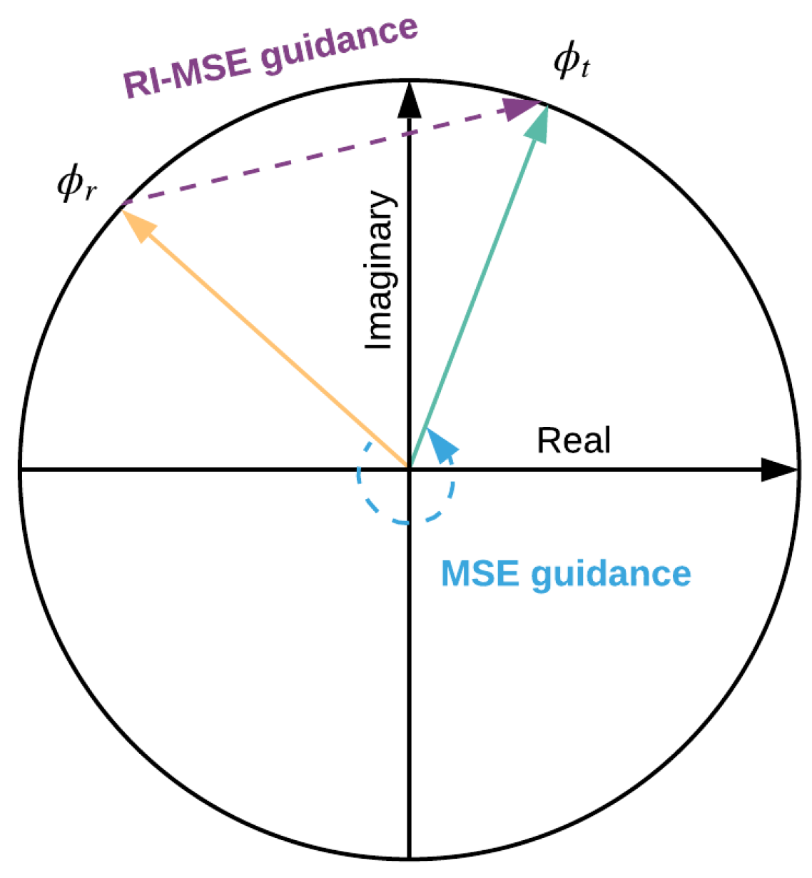
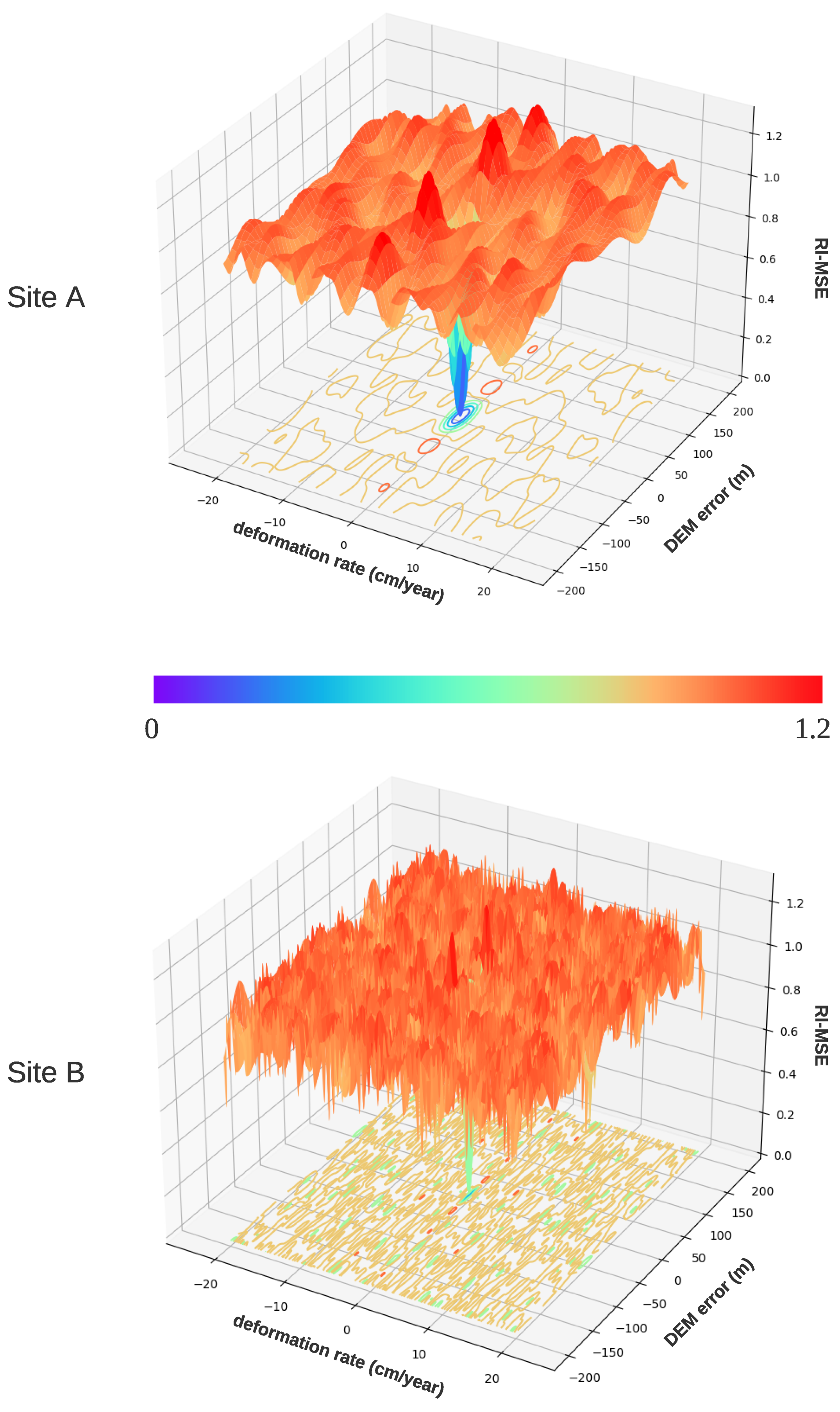
2.1. Mathematical Modelling for InSAR Phase

Interferometric phase modeling has been investigated in the literature [4,5,6,7]. Interferometric phase measurements are affected by various factors—imaging geometry, topography, atmospheric delay and ground deformation. For a given pixel location l in TSInSAR, interferometric phase can be represented in a differential interferogram [23] as follows:

$$\begin{array}{cc}\hfill {\varphi }_l& ={\varphi }_{def,l}+\Delta {\varphi }_{topo,l}+\Delta {\varphi }_{atmo,l}+\Delta {\varphi }_{orbit,l}+{\varphi }_{noise,l}\hfill \\ \hfill \widehat{{\varphi }_l}& =arctan2(sin\left({\varphi }_l\right),cos\left({\varphi }_l\right))\hfill \end{array}$$

(1)

where ${\varphi }_{def}$ represents phase components related to ground deformation motion, ${\varphi }_{topo}$ is the topographic phase contribution (DEM error when applied external DEM), ${\varphi }_{atmo}$ refers to the differences of atmospheric distortion between two single-look-complex (SLC) scenes, ${\varphi }_{orbit}$ denotes imprecise satellite orbit data when forward modeling the contributions of the Earth’s ellipsoidal surface, and ${\varphi }_{noise}$ describes decorrelation noise. The observed phase is also wrapped as $\widehat{{\varphi }_l}$. A general PSI processing chain eventually removes the flat-earth phase using satellite orbit data, and a collection of spatial and temporal filtering routines are adopted to reduce noise and remove other contaminant signals that are not deformation or DEM error [24,25,26]. Several established techniques are also described to mitigate the atmospheric phase contribution by deploying the toolbox for reducing atmospheric InSAR noise (TRAIN) [27,28]. It is known that both ${\varphi }_{orbit}$ and ${\varphi }_{atmo}$ could create long-scale correlated signals in the spatial domain. Hence, those phase contributions can be further reduced by giving double difference phase between two neighborhood PS pixels [9] as follows:

$$\begin{array}{cc}\hfill \Delta {\varphi }_{i,j}^k& =\Delta {\varphi }_{topo,(i,j)}^k+\Delta {\varphi }_{def,(i,j)}^{k}k=1,\dots ,N\hfill \end{array}$$

(2)

It describes the arc’s double difference phase constructed by a pair of PS pixels $i,j$ in interferogram k from a time-series stack with a length of N. In interferogram k, $\Delta {\varphi }_{topo,(i,j)}^k$ is the relative height between pixel i and j, and $\Delta {\varphi }_{def,(i,j)}^k$ is the relative deformation, respectively.

Furthermore, for each PS pixel, its topographic phase component can be modeled as a linear function of the spatial perpendicular baseline ($B_{\perp }$) according to the geometry relation of InSAR for each interferogram as:

$${\varphi }_{topo}^k=-\frac{4\pi }{\lambda }\frac{B_{\perp }^k}{R·sin\theta }·h=con{v}_{topo}·B_{\perp }^k·h$$

(3)

where $\lambda$ is the transmitted radar wavelength, R is slant range distance, $\theta$ denotes satellite incidence angle. Here, h is the orthometric height between two SLCs. We use $con{v}_{topo}$ to denote the unit conversion factor for a given stack. Similar to average ground deformation rate $\left(m_r\right)$, which is used for the modeling deformation phase as follows:

$$\begin{array}{cc}\hfill {\varphi }_{def}^k& =-\frac{4\pi }{\lambda }{(d^{first}-d^{second})}^k·m_r\hfill \\ \hfill & =-\frac{4\pi }{\lambda }\Delta day{s}^k·m_r\hfill \\ \hfill & =con{v}_{def}·\Delta day{s}^k·m_r\hfill \end{array}$$

(4)

where $\Delta days$ is the temporal baseline between two acquisitions on distinct days ($d^{first},d^{second}$) used to form the interferogram, and $con{v}_{def}$ is unit conversion factor. We can substitute Equations (3) and (4) into Equation (2), and then add an extra integer variable w to handle phase ambiguity between pixel i and j because of phase wrapping:

$$\begin{array}{cc}\hfill \Delta {\varphi }_{i,j}^k& =con{v}_{def}·\Delta day{s}^k·\Delta m_{r(i,j)}^k+con{v}_{topo}·B_{\perp }^k·\Delta h_{(i,j)}^k+2\pi ·w_{i,j}^{k}k=1,\dots ,N\hfill \end{array}$$

(5)

Due to the nature of microwave, the observed phase is wrapped as in Equation (1), there is an extra integer variable w that refers to phase ambiguity. It leads to N equations with more than N parameters that have to be resolved. That is why Equation (5) cannot be solved efficiently by a simple matrix inversion. As aforementioned, conventional PSI techniques consider this parameter fitting task as a two-dimensional regression problem or an integer optimization problem. Those methods try to map the integer least square (ILS) and two-dimensional solution search to the wrapped phase domain [14,15,29]. However, algorithms based on direct search are straightforward and do not require any complex modeling. They suffer from inefficient computation and are easily affected by local optima when dealing with complex baseline situation.

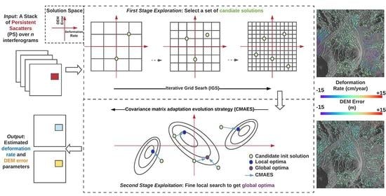
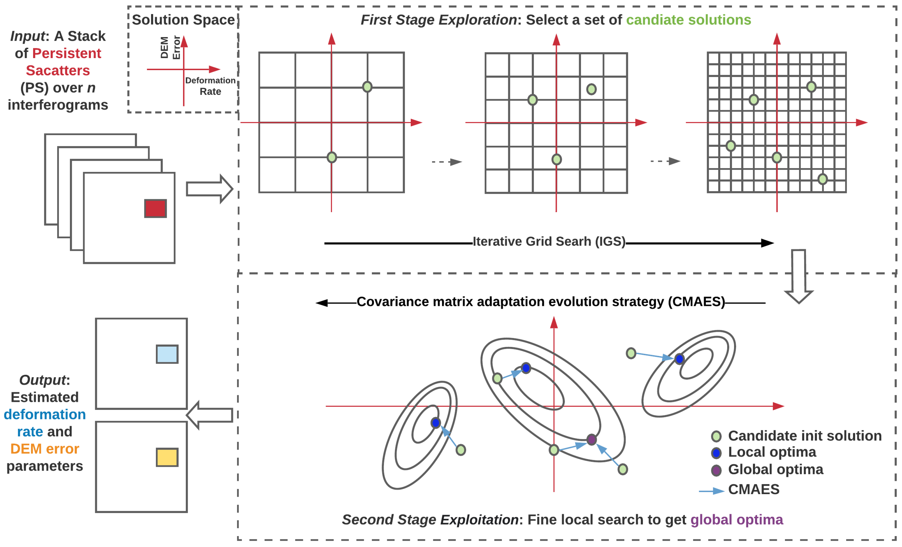
2.2. Proposed Method

2.2.1. Definition of Optimization Problem

In PSI frameworks such as DePSI (Delft PSI processing package) and StaMPS (Stanford method for persistent scatterers) [30,31], signal separation is one of the essential steps in the whole processing pipeline. Parameters estimation is applied in an iterative manner combined with a collection of spatial and temporal filtering routines to obtain a precise final estimate. A more efficient and accurate parameter estimation algorithm could accelerate the whole processing pipeline by reducing iterates. Detailed descriptions of PSI methodologies can be found in [1,23]. Our main focus is studying parameter estimation of linear deformation rate and DEM error upon PS time series, for the following reasons. (1) There are many state-of-the-art methods for filtering random noise and suppressing atmosphere components from a stack of interferograms [25,27,32,33,34]. (2) Recently, satellite facilities can provide accurate enough orbits for practical usage [35,36,37]. (3) It is very common to divide a complicated optimization problem into sub-problems, which are easier to be solved than the original problem [38,39]. (4) Arc-based methods have to apply prior knowledge to pick reference points and then resolve each coherent pair’s parameters [17]. The main limitation of these methods is that it only gives the relative signal estimation between two PS points, which requires prior known deformation information of at least one PS point to derive the final estimations. It might not be feasible in real scenarios, where there is no information about the monitoring area. Moreover, it may potentially introduce accumulated error when a poor reference point is selected.

Our preprocessed observed phase is already filtered, and the atmospheric phase and orbit phase have been removed using 3vGeomatics’s preprocessing chain described in [40]. The pre-removal of these two large spatial correlated signals allows us to work on each PS signal directly instead of using arcs. To this end, our phase model becomes:

$$\begin{array}{cc}\hfill {\varphi }^k& =con{v}_{def}·\Delta day{s}^k·m_r+con{v}_{topo}·B_{\perp }^k·h_{e}k=1,\cdots ,N\hfill \end{array}$$

(6)

Note that, we replace the h (height) with $h_e$ (DEM error), because we adopt external DEM to pre-remove the topographic phases. The outcome $h_e$ will be used to refine external DEM as $DE{M}_{refined}=DEM-h_e$. We define the average deformation rate and DEM error estimation problem as a two variables optimization task that consists of an objective function. Please note that DEM studied in this work is in range Doppler coordinates (RDC), which can be transformed to geographic coordinates by the geocoding step.

The objective of our optimization task is to minimize the residuals between observed target phase ${\varphi }_t$ and reconstructed phase ${\varphi }_r$, where ${\varphi }_r$ is calculated using Equation (6) with estimated $m_r$ and $h_e$. The typical objective functions for evaluating value difference in the continuous domain are mean absolute error (MAE) and mean square error (MSE). However, these Euclidean-based metrics are not suitable in the interferometric phase domain because of branch cuts. The value range of the wrapped phase is bounded by $[-\pi ,+\pi )$, which results in interferometric phase value jumping from negative to positive or positive to negative $\pi$. In this work, we consider the wrapped phase difference with real and imaginary MSE (RI-MSE) (Equation (7)).

$${\mathcal{J}}_{\beta }=\frac{1}{2N}\sum _{k=1}^N\left(\right(sin\left({\varphi }_o^k\right)-sin{\left({\varphi }_r^k\right)}^2+(cos\left({\varphi }_o^k\right)-cos{\left({\varphi }_r^k\right)}^2)k=1,\cdots ,N$$

(7)

As shown in Figure 1, there are two phasors (${\varphi }_t$ Green, and ${\varphi }_r$ Orange) plotted in a polar coordinate system. If we treat ${\varphi }_r$ as the reconstructed phasor and ${\varphi }_t$ as the target phasor, a Euclidean-based metric such as MSE would increase linearly with angle value difference. In terms of phase, the MSE objective function tends to guide the optimizer to move ${\varphi }_r$ anticlockwise as shown in Figure 1 (MSE guidance direction), especially when their difference is close to $\pi$. RI-MSE can be interpreted as the distance between two phasors on the unit polar coordinate circle. During optimization, the optimizer adjusts variables in order to force the reconstructed phasor close to the target phasor based on the perspective of projections on two axes. This approach has been commonly deployed as a good indication of wrapped phase distances in recent InSAR phase filtering studies [24,25,41].

At this point, our signal separation task is formulated as a parameter fitting problem by optimizing an objective function. As aforementioned, there are still N equations with more than N interferograms to be estimated for each pixel pair because of the wrapped phase. That is why Equation (5) cannot be solved efficiently by conventional methods. Previous studies [14,15,29] point out that although the direct search-based algorithms are simple without using complicated modeling, they suffer from local optima when dealing with complex baselines and large solution space.

We propose a two-stage algorithm that combines a global coarse searching followed by a fine local optimization. As shown in Figure 2, we first adopt an IGS policy to obtain a set of coarse candidate solutions, which are expected to approximate the global optima. We then apply CMAES for a fast fine local optimization starting with each candidate solution. Lastly, the best result with the minimal objective function value is picked as the final estimate.

2.2.2. CMAES

In [9], researchers tried to adopt a black-box optimizer—SA algorithm, to solve the deformation fitting optimization problem. Inspired by it, we propose to use CMAES [42] to take advantage of using gradient-free optimization for our task. CMAES is an evolutionary-based stochastic optimization algorithm, which has shown state-of-the-art performance in derivative-free optimization and performed best among more than 100 classic and modern optimizers on a wide range of black-box functions [43,44]. According to our phase model Equation (6), it can been seen that different temporal baselines ($con{v}_{def}$) and spatial baselines ($con{v}_{topo}$) result in very different objective functions. Its robust performance on optimizing unknown functions of CMAES is the major reason we choose it in our approach. When dealing with a few objective variables (two in our case), CMAES also obtains better speed than other methods [42,45,46]. A brief workflow of CMAES optimization is described as follows:

CMAES is an iterative algorithm, and there are three main steps in each iteration (t): (1) sample n candidate solutions from a multivariate normal distribution $N(m_t,{\sigma }_t^2{C}_t)$; (2) calculate function values for each sampling solution, (3) update the distribution parameters ($m_t,{\sigma }_t,C_t)$ accordingly. In this work, we use CMAES to minimize our loss function ${\mathcal{J}}_{\beta }$ (Equation (7)) with two objective variables $\widehat{\mathbf{v}}=[m_r,h_e]$ as shown below:

$$\widehat{\mathbf{v}}=\underset{\mathbf{v}}{\mathrm{argmin}}{\mathcal{J}}_{\beta }$$

(8)

We first give CMAES an initial solution point as a start searching location $v_0=\left[m_{r\left(0\right)},h_{e\left(0\right)},\right]$ with an initial sampling distribution $N_0(m_0,{\sigma }_0^2{C}_0)$, where $m_0=v_0$, $C_0=I\in {\mathbb{R}}^2$ and ${\sigma }_0$ denotes the initial step size, which is set to 0.01 in our study. Then, at each iteration t we generate S candidate solutions $v_k$ sampled from $N_t$ as:

$$v_k=m_t+{\sigma }_t{y}_k,y_k\sim N(0,C_t)$$

(9)

where k is the index of the randomly sampled candidate solutions with a total number of S. Here, each $y_k\in {\mathbb{R}}^2$ can be treated as a searching direction. Next, calculate all candidate solutions’ objective function values $\mathcal{J}\left(v_k\right)$ and sort them as:

$$\mathcal{J}\left(v_{1:S}\right)\le \mathcal{J}\left(v_{2:S}\right)\le \cdots \le \mathcal{J}\left(v_{S:S}\right)$$

(10)

The subscript indicates the rank of those samples out of S. The optimizer will stop if the best solution reaches the termination criteria $\mathcal{J}\left(v_{1:S}\right)<\tau$, where $\tau$ is a threshold, which is set with a small value ${10}^{-11}$. Otherwise, it uses the top $\mu$ ($\mu <S$) solutions to update the distribution parameters. Note that the rank order is only based on comparing the objective function itself, known as objective value-free ranking. In this work, we select top $\mu =\lfloor {\displaystyle \frac{S}{4}}\rfloor$ solutions with the lowest objective functions to update distribution parameters $m_t$ and $C_t$, where the mean of the new distribution $m_{t+1}$ is updated as

$$m_{t+1}=\sum _{k=1}^{\mu }{w}_k{v}_{k:S}=m_t+\sum _{k=1}^{\mu }{w}_k(v_{k:S}-m_t)$$

(11)

If we set $w_k={\displaystyle \frac{1}{\mu }}$ for all candidate solutions, then the updates are treated as the maximum-likelihood estimation of all selected solutions. In this work, we want to emphasize the solutions with the lowest objective function and defined the function below as our weighting function:

$$w_i=1-{\displaystyle \frac{\mathcal{J}\left(v_{k:S}\right)}{{\sum }_{k=1}^{\mu }\mathcal{J}\left(v_{k:S}\right)}}$$

(12)

In this case, the updates in Equation (11) can be treated as a stochastic approximation of the natural gradient of m, which is recently used for optimizing deep neural networks on a reinforcement learning task [47]. The covariance matrix C is updated using:

$$p_{t+1}=(1-c)p_t+\sqrt{c(2-c)}\sqrt{{\mu }_w}{\displaystyle \frac{m_{t+1}-m_t}{{\sigma }_t}}$$

(13)

$$C_{t+1}=(1-c_1-c_{\mu })C_t+c_1{p}_{t+1}{p}_{t+1}^{⊺}+c_{\mu }\sum _{k=1}^{\mu }{w}_k{y}_{i:S}{y}_{k:S}^{⊺}$$

(14)

where p can be treated as the evolution path, which is 0 at the beginning and ⊺ is the symbol for vector transpose. It is similar to a mutation used for updating covariance matrix, and c is the learning rate for updating p. We set $c=0.5$, which is the number of variables divided by 4 as recommended in [48]. ${\mu }_w$ is equal to ${\displaystyle \frac{1}{{\sum }_{i=1}^{\mu }{w}_i^2}}$, which is used for weighting intermediate recombination to force the second term as a random vector selected from $N(0,C_t)$. $c_1$ and $c_{\mu }$ are two other learning rates which are set to be ${\displaystyle \frac{2}{n^2}}=0.5$ and ${\displaystyle \frac{{\mu }_w}{n^2}}$, respectively. To update step size $\sigma$, we adopt CMEAES’s default cumulative step size adaption (CSA):

$$s_{t+1}=(1-c_{\sigma })s_t+\sqrt{c_{\sigma }(2-c_{\sigma })}\sqrt{{\mu }_w}{C}^{-{\displaystyle \frac{1}{2}}}{\displaystyle \frac{m_{t+1}-m_t}{{\sigma }_t}}$$

(15)

$${\sigma }_{t+1}={\sigma }_{t}exp({\displaystyle \frac{c_{\sigma }}{d_{\sigma }}}({\displaystyle \frac{\parallel s_{t+1}\parallel }{\mathbb{E}\parallel N(0,I)\parallel }}-1))$$

(16)

where s is another conjugate evolution path that is similar to p but ignoring the scale fact. $c_{\sigma }$ and $d_{\sigma }$ are two parameters for controlling the changing magnitude of $\sigma$ are set to ${\displaystyle \frac{2}{n^2}}=0.5$ and $1+\sqrt{{\displaystyle \frac{{\mu }_w}{n^2}}}$, respectively. We adopt the default configuration defined in the literature [49] for this study, and the key parameters of the CMAES algorithm are listed in

Table 1. The key parameters of covariance matrix adaptation evolution strategy (CMAES) used in this work.

Parameter	Definition	Value
S	Number of candidate solutions at each iteration	30
${\sigma }_0$	Initial step size	0.01
$\mu$	Number of selected top ranked solutions	7
$\tau$	Threshold value to terminate the optimization	${10}^{-11}$
c	Learning rate for updating evolution path	0.5
$c_1$	Learning rate for updating covariance matrix	0.5
$c_{\sigma }$	Learning rate for updating step size	0.5

.

Once the distribution parameters are updated, the optimizer will start another new iteration until it reaches the termination condition. The main advantage of CMAES over classical ES is the use of correlated mutations instead of axis-parallel ones. It can learn appropriate mutation distribution steadily and has a high probability of reaching optima by using adapted covariance matrix C to adjust searching direction [45]. However, CMAES is still a local search optimizer similar to SA and many other stochastic optimizers. They may get stuck in local optima, and the convergence to global optima is not guaranteed [44,48]. Many works have pointed out that the initial search position is essential for stochastic optimization. Restart-based methods are very classical but useful in many optimization frameworks and show benefits in finding the global optima. There are also many CMAES extensions [43] using restart strategies to prevent premature convergence on complicated tasks. The main limitation of those approaches is that they need extra search in the hyper-parameter space of the population size, and the initial step-size seems inefficient. Moreover, the subsequent restarted search usually relies on previous search results, making the whole optimization process hard to be parallelized. However, there is evidence to support the fundamental idea behind restarts; the initial search location is essential for finding the global optima and saving the computations. To address these issues, we propose a pre-stage exploration search for picking a set of potential candidate solutions for CMAES. Then, CMAES will use those initial solutions for fine local optimization as the second exploitation stage.

2.2.3. Iterative Grid Search (IGS)

To find good candidate solutions for fine local optimization, we introduce an IGS strategy in this work. In Figure 3, we examine the loss landscapes computed using Equation (7). We inject 0 deformation and 0 DEM error as ground truth with two site baseline parameters ($con{v}_{def},con{v}_{topo},\Delta days,B_{\perp }$) for generating simulated wrapped interferogram using Equation (6). We then oversample both deformation rate (1000 samples) and DEM error (1000 samples) to better illustrate the surface of the corresponding loss value landscape ($1e6$ evaluated solutions). By observing Figure 3, it can be seen that both landscapes are non-convex, rugged and contain many local optima. This is the reason why a simple gradient-based optimizer is hard to find global optima. The desired algorithm is expected to converge to global optima effectively and avoid brute force grid search because naïve sampling is impractical when high precision estimation and real-time performance are required. Comparing landscapes of the two sites also shows that different real-world baselines could result in very distinct objective functions. Some site baseline parameters may produce much more challenging objective functions than others.

In fact, a straightforward grid search is commonly used in industry processing pipelines. For a $\pm 26$ cm/year linear deformation rate and $\pm 200$ m DEM error study case, a typical grid search is applied as $S_s$ with $0.5$ cm and 2 m step size (respective to deformation rate and DEM error) in order to pick the best solution. It generates $(2\times 200/2)+(2\times 26)/0.5$ = 20,800 number of objective function evaluations in total for each PS location and has a limited precision bottleneck regarding the step size. Increasing the step size can reduce the computations but also decrease the precision. Furthermore, a large step will result in poor estimation for complicated baselines because of the objective function’s ruggedness. We treat $\kappa S_s$ as sampling step size for deformation rate and DEM error, where a scaling factor $\kappa$ is used to control the density of grid search. In an optimization task, the number of objective function evaluations (search cost) is an essential metric for assessing a stochastic optimizer’s performance. Especially when higher precision is required, dense grid search is extremely insufficient. Moreover, from an optimization point of view, determining whether the true global optima reached is a fundamental challenge as a stochastic optimization algorithm. As a consistency check, the algorithm can be run from several different random starting points to ensure the result of each run converges to the global optimal. Rather than using randomly selected starting points, in this work, we hypothesize that using a low-precision grid search can select a set of initial candidate solutions that are potentially close to the global optima. To support our assumption, we plot the loss landscapes with different sampling steps sizes by setting $\kappa =[1,3,5,8]$ as shown in Figure 4.

By observing the resulting loss landscapes at different sampling scales, we notice that global optima can be roughly located with a less dense grid sampling. As seen in Site-A and Site-B from Figure 4, $\kappa =5$ or 8 is sufficient to estimate the location of global optima. However, when dealing with complicated baselines such as Site-C and Site-D, it is necessary to require $\kappa =1$ or 3 in order to roughly locate the optimal solution. A large sampling step size (large $\kappa$) leads to low precision, but a small sampling rate (small $\kappa$) brings massive computations. Figure 4 shows that there is no fixed optimal sampling scale $\kappa$ for different baselines. Hence, in this work, we propose an iterative strategy by performing grid sampling from large $\kappa$ to small units until N acceptableinitial solutions have been picked. We define a threshold $\omega$ for accepting sampled estimates, whose values are less than $\omega$ as acceptable initial solutions.

IGS performs grid sampling with different $\kappa$ iteratively, and the key steps at each iteration are: (1) sort all sampled estimates based on their loss values (Equation (7)); (2) if the smallest one is greater than $\omega$, the algorithm will iterate to the next grid search level. Otherwise, it pushes the estimate to candidate solution list one by one until the length of N or no solution loss is less than $\omega$. Moreover, solutions close to global or local optima might have similar loss values, as shown in Figure 5 (Estimate C, 2, 3). To avoid selecting solutions from the same local area in the landscape, we define a $CheckDistance$ procedure to skip solutions that are too close to any existing accepted solutions. A threshold value $\psi$ is adopted to determine if two solutions are too close to each other by assessing two estimates L2 distances in the solution space. As shown in Figure 5, if point C is already labeled as a candidate solution, points 2 and 3 will not be considered. Instead, the algorithm will consider points 4 and 5 because they are not close to any existing candidate solution.

2.2.4. IGS-CMAES

Once we get a certain number of acceptable initial solutions, CMAES is then applied for local fine optimization. In fact, there are existing CMAES extension works that are proposed based on a repeat mechanism. The key concept of those methods is repeating CMAES process by adjusting the initial point and population size according to the results from previous runs. They offer better performance but increase the computation time because the adjustments are not parallelizable. In our work, CMAES runs only once for each candidate solution as a starting location. Hence, the local search can be performed in parallel to save overall execution time compared to repeat-based algorithms. Our complete IGS-CMAES optimization procedure is given in Algorithm 1.

Algorithm 1: IGS-CMAES for deformation rate and DEM error estimation.

To summarize, we propose to use IGS to globally select acceptable initial solutions, which are with high possibility of close to the global optima. We then apply CMAES, started from each selected initial solution, to perform the local refine search. Lastly, the final result is the best estimate among all local solutions. Overall, IGS-CMAES can save unnecessary function evaluations compared to dense grid search but still cover the global optimal space. At the same time, it also preserves the benefits of accuracy and efficiency from the local search.

3. Results

3.1. Experimental Setup

This section empirically demonstrates the effectiveness and robustness of the proposed IGS-CMAES using both simulated and real-world TSInSAR data. All our experiments are based on seven real-world stacks R (R1–R7), captured by TerraSAR-X in StripMap mode [50]. Each stack represents a different ground site and contains 31 SLCs except R7, which has 17 SLCs. We designed a simulator that generates TSInSAR signals by injecting synthetic deformation rate and DEM error with real-world baseline parameters. Moreover, we apply an industry 3vGeomatics’s industry-standard InSAR processing pipeline [40,51] to perform data preprocessing as well as generate the reference results to assess the performance of the proposed IGS-CMAES method on real data. The experiments were designed to estimate two important parameters: optimization cost and accuracy. Optimization cost is defined as the number of objective function evaluations. Accuracy is assessed directly by comparing with synthetic deformation rate and DEM error values in the simulation setup. Because there is no ground truth in the real-world scenario, we adopt mean phase residual (MPR) between the wrapped reconstructed and input interferograms to evaluate performance. The details of both experiments and results are presented in the following sub-sections, and the code is available at: https://github.com/Lucklyric/TSInSAR-PF-IGS_CMAES (accessed on 23 June 2021).

3.1.1. Simulation Data

Our simulator generates interferometric phase by injecting synthetic deformation rate and DEM error into seven real-world temporal and spatial baselines R1–R7. For each dataset, in order to assess the robustness of different optimizers, we sample 30 deformation rates and 60 DEM errors from two uniform distributions—$\mathcal{U}(-26,26)$ cm/year and $\mathcal{U}(-200,200)$ m. It gives a total of 1800 possible signal pairs for each of the seven baselines, which are further used to generate synthetic interferometric pixel stacks using Equation (6), where $con{v}_{def}$, $\Delta days$, $con{v}_{topo}$ and $B_{\perp }$ are real-world baselines from the R1–R7 stacks. In order to objectively evaluate different methods, we use (1) root-mean-square error (RMSE) between the simulated (ground truth) and the estimated deformation rate (cm/year) and DEM error (m), (2) L1 unwrapped phase difference (L1-UPD) between the simulated (unwrapped ground truth) and the reconstructed phase calculated based on the estimated deformation rate and DEM error, (3) the accuracy (ACC%) of reducing rate that counts the percentage of how many test cases that the method’s unwrapped L1 phase error is less than $\pi$. We performed our experiments from three perspectives: (1) apply four widely used local optimizers—(a) least square (LS), (b) Nelder–Mead [52], (c) conjugate gradient (CG) [53] and (d) Broyden–Fletcher–Goldfarb–Shanno (BFGS) [54], to show how challenging our task is when applying conventional local optimizers; (2) adopt the IGS strategy into all local optimizers used in the first experiment to showcase the improvements in comparison with our coarse search strategy; (3) compare to the other two global optimization methods—direct gird search (baseline method) and dual simulated annealing (Dual-SA) [55]—to investigate the novelty of our IGS-CMAES algorithm.

From

Table 2. Quantitative assessment for simulated data with several widely used local optimizers and their IGS-extended version.

Baseline	Categories	LS	IGS- LS	Nelder- Mead	IGS- Nelder- Mead	CG	IGS- CG	BFGS	IGS- BFGS
R1	$m_r$-RMSE (cm/year)	12.2382	2.9481	12.4695	2.0734	12.5197	1.3484	12.4414	1.2893
	$h_e$-RMSE (m)	107.0381	0.0011	105.6981	0.0001	107.6607	0.0000	106.5213	0.0000
R2	$m_r$-RMSE (cm/year)	13.2260	2.3247	13.3805	2.5936	13.6642	1.3439	13.6011	1.3143
	$h_e$-RMSE (m)	107.2283	0.0016	106.3737	0.0002	107.4976	0.0000	107.5918	0.0000
R3	$m_r$-RMSE (cm/year)	13.0308	1.9413	13.1002	1.6877	13.3366	1.4307	13.2444	1.0897
	$h_e$-RMSE (m)	107.8291	0.0016	106.5126	0.0002	108.3554	0.0000	108.7696	0.0000
R4	$m_r$-RMSE (cm)	12.7119	1.9372	13.1455	2.2679	13.1560	0.8951	13.2614	2.0387
	$h_e$-RMSE (m)	107.5101	0.0032	106.5326	0.0002	108.2290	0.0000	108.4366	0.0000
R5	$m_r$-RMSE (cm/year)	12.6042	2.1055	12.6375	1.9330	12.8295	0.8136	12.8457	1.5362
	$h_e$-RMSE (m)	106.7188	0.0022	105.9384	0.0002	109.1707	0.0000	107.6000	0.0000
R6	$m_r$-RMSE (cm/year)	12.4571	1.9549	12.5720	1.7121	12.5872	0.6817	12.6906	0.7807
	$h_e$-RMSE (m)	105.3393	0.0062	106.0447	0.0003	108.2960	0.0000	109.1020	0.0000
R7	$m_r$-RMSE (cm/year)	12.5991	14.9993	12.6070	14.1472	12.7588	6.7126	12.6561	3.2887
	$h_e$-RMSE (m)	106.6014	0.0006	106.0582	0.0001	108.0011	0.0000	12.6561	0.0000

, it is obvious that none of the local optimizes works for any stack. They show significant errors on both types of signal estimation. During the experiments, all local optimizers prone to converge to local optima around the initial solution. However, comparing to IGS-extended versions, which run each local optimization following IGS policy, there is a consistent agreement to reduce the errors in deformation and DEM error estimations. As shown in Figure 6 and Figure 7, a significant decrease in L1-UPD and improvement in ACC is observed, when IGS is adopted. The proposed IGS policy effectively improves all local optimizer performance in the unwrapped phase domain, except R7, which is a special case with fewer SLCs. Nevertheless, all IGS-optimizers produce acceptable results. However, due to the limitation of those local optimizers themselves, the results are still not satisfactory.

In this work, we also provide comparison between the proposed IGS-CMAES and other two global algorithms—grid search and Dual-SA with an extra metric—the mean number of objective function evaluation (NFev). Both methods are designed for global optimization. The comparisons reported in

Table 3. Quantitative comparison for simulated data using IGS-CMAES with two other global optimizers.

Baseline	Categorie	IGS-CMAES	Grid-Search	Dual-SA
R1	$m_r$-RMSE	0.0284	0.0967	0.6336
	$h_e$-RMSE	0.0000	0.5611	31.7574
	L1-UWPD	0.0424	0.1191	1.3113
	ACC	99.94%	100%	96.88%
	NFev	2725.03	20800	4109.38
R2	$m_r$-RMSE	0.1137	0.0967	0.1792
	$h_e$-RMSE	0.0000	0.5610	6.7533
	L1-UWPD	0.0424	0.1051	0.1279
	ACC	99.94%	100%	99.35%
	NFev	2585.18	20800	4103.06
R3	$m_r$-RMSE	0.1991	0.0967	0.4899
	$h_e$-RMSE	0.0000	0.5613	15.5361
	L1-UWPD	0.0791	0.1180	0.7239
	ACC	99.61%	100%	96.33%
	NFev	2687.90	20800	4112.38
R4	$m_r$-RMSE	0.2276	0.0967	0.0588
	$h_e$-RMSE	0.0000	0.5617	7.5336
	L1-UWPD	0.0848	0.0806	0.0534
	ACC	99.56%	100%	99.69%
	NFev	2500.69	20800	4089.58
R5	$m_r$-RMSE	0.2844	0.0967	0.1556
	$h_e$-RMSE	0.0000	0.5617	5.8893
	L1-UWPD	0.1065	0.0864	0.0853
	ACC	99.44%	100%	99.52%
	NFev	2520.12	20800	4093.36
R6	$m_r$-RMSE	0.0000	0.0967	0.0000
	$h_e$-RMSE	0.0000	0.5617	0.0000
	L1-UWPD	0.0000	0.0591	0.0000
	ACC	100%	100%	100.00%
	NFev	2381.48	20,800	4070.47
R7	$m_r$-RMSE	1.6145	7.763333	13.902
	$h_e$-RMSE	0.0000	0.5609	104.1441
	L1-UWPD	1.1259	5.5327	27.8864
	ACC	94.88%	70%	39.03%
	NFev	3576.92	20800	4121.54

show that all three methods have an on-par accuracy on deformation estimation when using R1-R6. However, Dual-SA fails to give proper estimates of DEM error except for R6. The error of grid search is mainly due to its limited sampling precision and it fails to provide proper deformation estimation when working on limited temporal information R7, which also troubles Dual-SA. In contrast, our IGS-CMAES consistently offers robust and accurate results, and achieves better generalization ability than other two methods. Furthermore, IGS-CMAES has demonstrated a significant improvement in NFev by saving more than 85% objective function computation costs compared to grid search, while maintaining similar and even better results. Our method surpasses Dual-SA on all baselines with substantial improvement in both accuracy and efficiency.

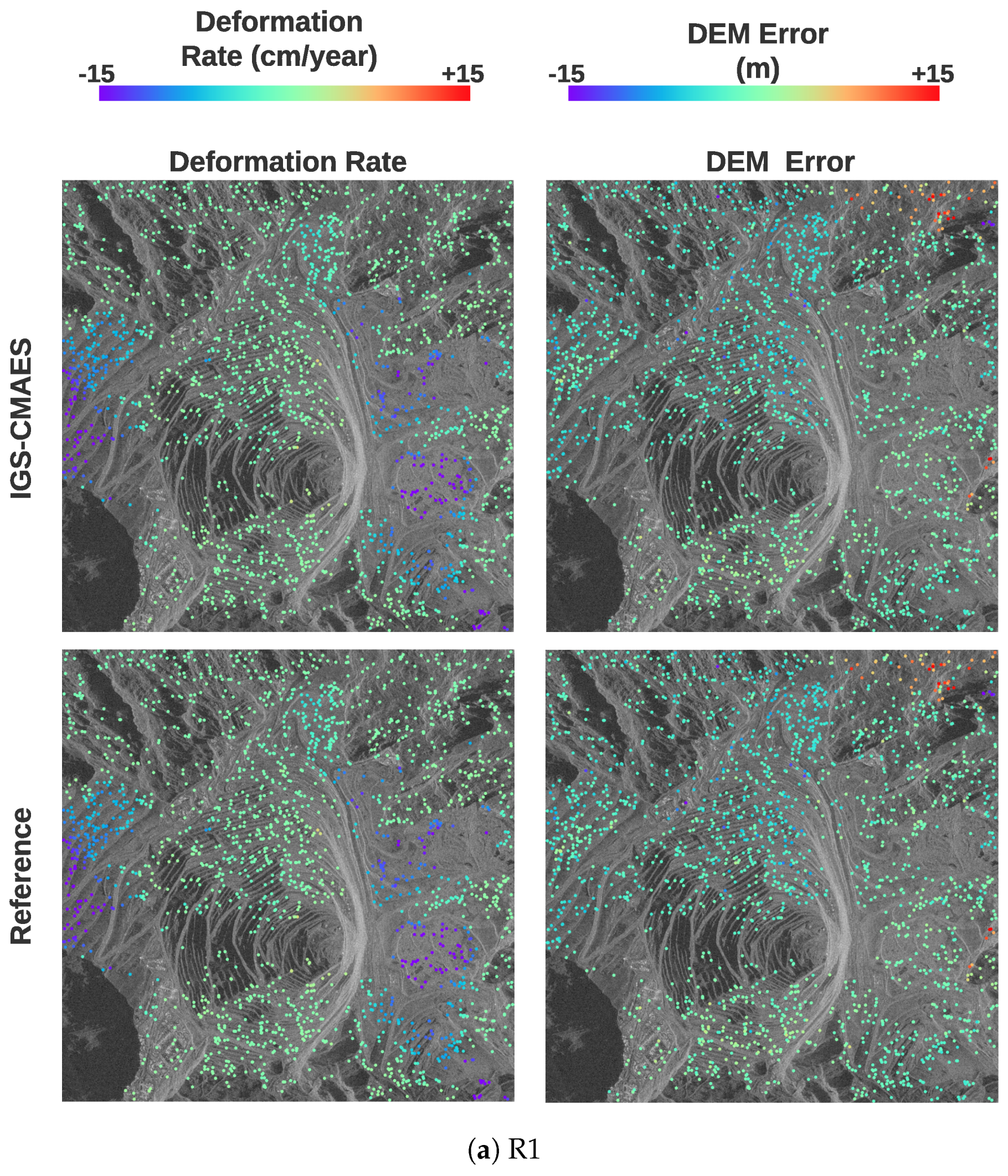
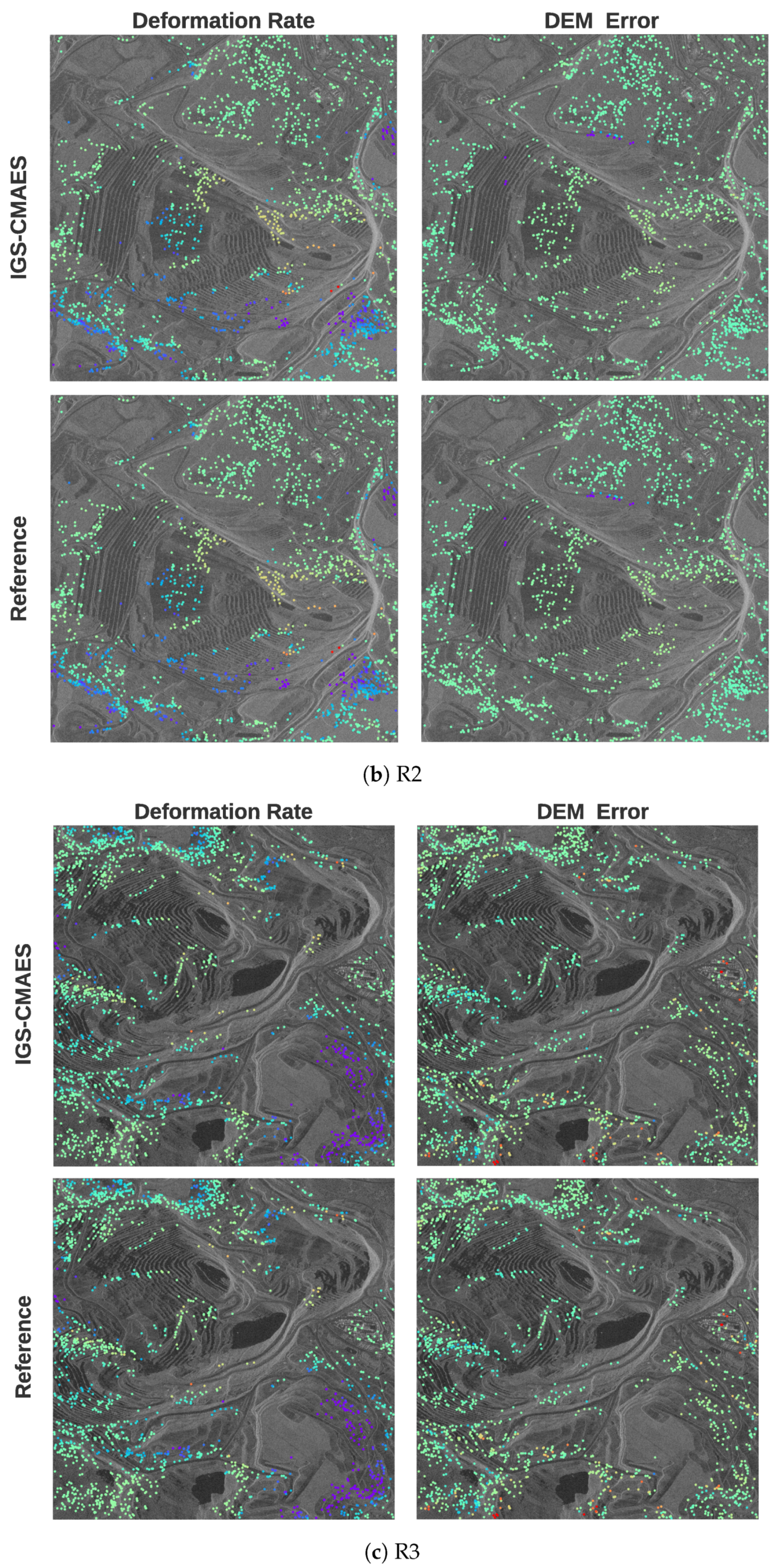
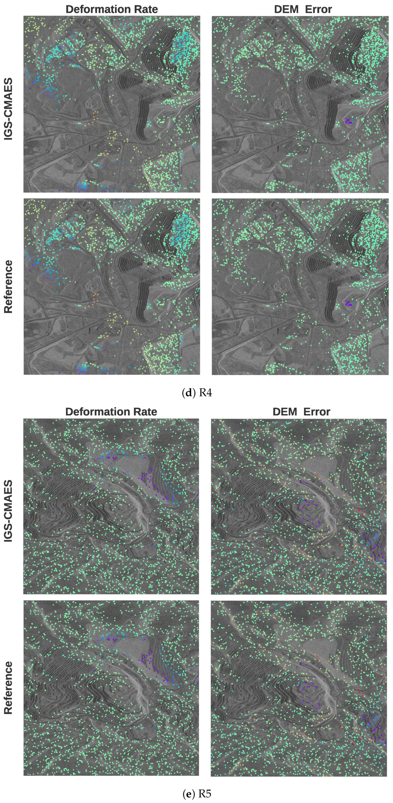
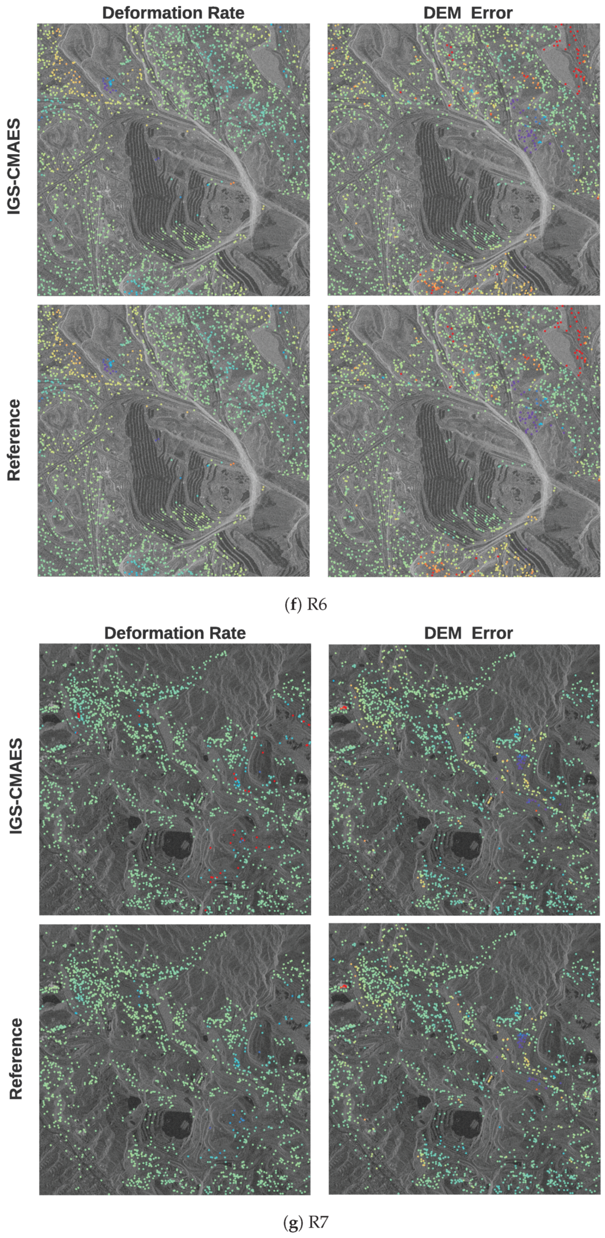
3.1.2. Real-World Data

In this section, we present results obtained when applying IGS-CMAES to real interferometric SAR acquisitions. All input interferograms from the R1–R7 have been preprocessed by the 3vGeomatics processing pipeline [40] with proper filtering, earth flattening and atmospheric phase removal as discussed in Section 2.2.1. There are 2000 PS pixels selected from each stack, which results in 14,000 test data points. Because there is no ground-truth data for real-world data, we adopt the final results from the processing pipeline as reference output. Such pipeline involves a phase unwrapping step and then uses least-square optimization to approximate the linear deformation rate and DEM error on the unwrapped phase directly. Phase unwrapping is known to be very time-consuming, but we can treat those outputs as reference results. It is worth mentioning that our proposed IGS-CMAES is designed to work on the wrapped phase directly in order to save the computations in unwrapping.

We estimate the linear deformation rate end DEM error using the proposed model on selected PS locations. Visual outputs and comparison to the reference results can be found in Figure 8. It is shown that the estimates of IGS-CMAES match the reference output pretty well in R1-R6. There are a few apparent disagreements on deformation rate in R(7), where reference results indicate small movements, but IGS-CMAES predicts high positive displacements (red dots). After careful examination, we present our numerical analysis in

Table 4. Quantitative assessment of IGS-CMAES’s outputs with reference results.

Baseline	NFev	RI-MSE Proposed (Rad)	RI-MSE Reference (Rad)	WPR IGS-CMAES (Rad)	WPR Reference (Rad)	${\mathit{m}}_{\mathit{r}}$-RMSE (cm)	${\mathit{h}}_{\mathit{e}}$-RMSE (m)
R1	4023.67	0.305124	0.307999	0.431716	0.435595	0.114381	0.061021
R2	3960.59	0.306338	0.307771	0.438660	0.439584	0.080547	0.053405
R3	3872.19	0.238092	0.242657	0.371183	0.374736	0.109501	0.052438
R4	3510.90	0.120080	0.119850	0.238335	0.238453	0.034719	0.048583
R5	3563.92	0.120687	0.122859	0.249803	0.250186	0.059676	0.122966
R6	3496.90	0.161789	0.161793	0.321250	0.321475	0.025550	0.102940
R7	3817.64	0.191073	0.210659	0.326159	0.352141	0.190598	0.061347

. We calculate $m_r$-RMSE and $h_e$-RMSE to quantify the difference between the IGS-CMAES and reference results. The only significant mismatch is the deformation rate in R7 (0.190598), which correlates with the observation in Figure 8. All other categories stay commensurate with a little disparity. We further investigate the wrapped phase residuals (WPR) between the wrapped reconstructed phase and input interferogram, and our method shows lower residuals than the reference output. This finding can also be confirmed by checking RI-MSE (Equation (7)), which is presented to show the phase distance in the polar coordinate system (Figure 1). Experimental results reveal that our IGS-CMAES offers more performance advantages on global convergency than the reference output. Moreover, our method can be applied to wrapped interferograms directly while achieving equal performance compared to the reference method, which requires phase unwrapping. Lastly, the algorithm continuously performs around 3800 NFev for each baseline. Therefore, we are confident that IGS-CMAES can serve as an efficient optimizer and provide accurate global fitting.

4. Discussion

Average ground deformation rate and DEM error estimation concurrently using TSInSAR stack can naturally be treated as a two-dimensional optimization task. However, due to the wrapped phase, the resulted objective function could contain many local optima that results in a pure local optimizer easily stuck to semi-optimal solutions. Moreover, varying spatial and temporal baseline parameters ($con{v}_{def}$, $\Delta days$, $con{v}_{topo}$ and $B_{\perp }$) also lead to different objective functions to be resolved. Hence, both global convergence and generalization ability are considered in our method. The proposed IGS policy tackles this optimization problem by iteratively sampling to select candidate solutions at a coarse level. It avoids inefficient naïve grid search but also retains a global exploration. Our simulation experiments confirm the benefits of the proposed IGS policy in Table 2 and Figure 6 and Figure 7. The failing local optimizers tend to exhibit significant improved results after IGS boosting. However, due to the bottlenecks of local optimizers, their results can only be as good as dense grid search and Dual-SA (Table 3).

Under the scope of global optimization, the performance of naive dense grid search highly relies on the sampling step size. An inevitable trade-off between precision and computation efficiency limits its usage when millimetric accuracy is required. SA algorithm is demonstrated in a recent study [9] on small-scale motion detection, which inspires us to adopt a stochastic gradient-free optimizer in this work. Its global extension Dual-SA combining Classical SA, and Fast SA has shown better results than other conventional optimizers. However, SA-based methods highly depend on randomness, and Dual-SA’s global search policy relies on hyperparameter tunning to generalize to different objective functions [43,55]. It can be observed from Table 3, that Dual-SA results show unstable performance when dealing with different baselines. In contrast, CMAES leads to fast local convergence with adaptive searching direction using the covariance matrix and has shown superior performance on many local optimization benchmarks. In addition, we can achieve fast convergence with CMAES by setting a small population size and step size because we have conducted sufficient exploration during the first IGS stage. At the second stage of optimization, CMAES can directly focus on local optimization for exclusive exploitation.

In our real data experiments, reference results are generated by 3vGeomatics’s industry level processing pipeline. The pipeline has served industry customers for years, and it is reasonable to treat its outputs as empirically validated references. Besides its robustness, this pipeline requires phase unwrapping to eliminate phase ambiguities before signal estimation. As aforementioned, phase unwrapping itself is an expensive step and has a dependency on prior known displacement pixel as the reference [17]. Due to our data nature, where no ground truth is available, it does not allow us to perfectly assess IGS-CMAES’s estimates. Hence, we use reference results that are based on wrapped phase. The proposed IGS-CMAES achieves a comparable output but on wrapped phase directly. It substantially improves existing work by skipping the complicated unwrapping step and preserve a robust estimation.

Lastly, we want to discuss the disagreement in the R7 stack, which shows a few miss-matched estimations between IGS-CMAES and the reference output. This is an interesting finding, as the statistics in Table 4 suggest that IGS-CMAES has very similar results as the reference one on all other stacks. Though significant differences happen in R7, IGS-CMAES shows consistent lower phase residuals between the wrapped and input phases. To this end, we can only conclude that the proposed IGS-CMAES provides robust convergence from an optimization point of view. However, our optimization tasks and objective function are defined following the literature of the linear deformation model. It is worth mentioning that R7 is the only stack with just 17 SLC acquisitions comparing to all other stacks (31 SLC). A limited number of terms in Equation (7) results in a potential situation that the objective function’s optimal solution might not cover all the latent truth estimates. The hyperthesis might not hold due to insufficient temporal information resulting in overfitting of the data, but the unwrapping used for generating the reference phase provides a spatial regularization that reduces the amount of overfitting. Fortunately, enough number of SLC acquisitions results in more formatted interferograms—which is commonplace nowadays to obtain sufficient SLCs for one site. Reference results are based on the unwrapped phase, and phase unwrapping is a step that incorporates spatial analysis, which is not the scope of this work. However, considering spatial analysis can reduce the effect on limited temporal access. This understanding guides us to incorporate both spatial and temporal analysis for deformation and DEM error estimation in future work. Overall, based only on temporal analysis, IGS-CMAES delivers robust results on stacks with sufficient temporal observations. Its effectiveness in solving optimization tasks is well validated in our method by using both simulation and real data experiments.

5. Conclusions

Estimating ground deformation and DEM error with TSInSAR data is an ill-posed problem. In this work, we provided two main contributions: (1) designing a two-stage architecture suitable for interferometric phase processing and (2) introducing a benchmark hybrid simulation dataset by combing real-world baseline parameters and synthetic ground truth signals for an effective evaluation. It is known that, when the availability of exclusive time series data increases, it is necessary to design more efficient and effective algorithms. Typically, research in these fields is conducted by solving complex optimization problems, which are extremely computationally intensive and time-demanding. By considering parameter estimation as an optimization problem, we presented an exploration process to acquire sufficient global information that will guide us to the optimal solution using IGS coarse search. After that, a group of candidate solutions is passed to the second exploitation step, where the best estimation is obtained using an effective local CMAES refined search. The combined two-stage optimization delivers a high degree of accuracy and efficiency without being influenced by local extrema. Our method was evaluated using simulated and real data, and the result outperforms traditional local and global optimizers. Furthermore, IGS-CMAES offers the advantage of avoiding phase unwrapping, which is often time-consuming and prone to error. It also generalizes well to different real site baselines without retuning the model configurations. In conclusion, this study demonstrates that our proposed two-stage black-box optimization framework IGS-CMAES successfully addresses two research tasks concurrently: linear deformation estimation and DEM error correction with TSInSAR data. When sufficient temporal information is provided, investigations on real data demonstrate that IGS-CMAES achieves comparable performance to an industry-standard processing pipeline, which requires a phase unwrapping process. Further developments of this work will focus on the improvements by considering spatial information when dealing with limited temporal data.

References

1. Sousa, J.J.; Hooper, A.J.; Hanssen, R.F.; Bastos, L.C.; Ruiz, A.M. Persistent Scatterer InSAR: A comparison of methodologies based on a model of temporal deformation vs. spatial correlation selection criteria. Remote Sens. Environ. 2011, 115, 2652–2663. [Google Scholar] [CrossRef]
2. Usai, S. The use of man-made features for long time scale insar. In Proceedings of the IGARSS’97. 1997 IEEE International Geoscience and Remote Sensing Symposium Proceedings. Remote Sensing—A Scientific Vision for Sustainable Development, Singapore, 3–8 August 1997; Volume 4, pp. 1542–1544. [Google Scholar]
3. Hooper, A. A multi-temporal InSAR method incorporating both persistent scatterer and small baseline approaches. Geophys. Res. Lett. 2008, 35. [Google Scholar] [CrossRef] [Green Version]
4. Reza, T.; Zimmer, A.; Blasco, J.M.D.; Ghuman, P.; Aasawat, T.K.; Ripeanu, M. Accelerating persistent scatterer pixel selection for InSAR processing. IEEE Trans. Parallel Distrib. Syst. 2017, 29, 16–30. [Google Scholar] [CrossRef]
5. Ferretti, A.; Prati, C.; Rocca, F. Nonlinear subsidence rate estimation using permanent scatterers in differential SAR interferometry. IEEE Trans. Geosci. Remote Sens. 2000, 38, 2202–2212. [Google Scholar] [CrossRef] [Green Version]
6. Zhang, L.; Ding, X.; Lu, Z. Modeling PSInSAR time series without phase unwrapping. IEEE Trans. Geosci. Remote Sens. 2010, 49, 547–556. [Google Scholar] [CrossRef]
7. Hu, F.; Wu, J. Improvement of the multi-temporal InSAR method using reliable arc solutions. Int. J. Remote Sens. 2018, 39, 3363–3385. [Google Scholar] [CrossRef]
8. Bekaert, D.; Walters, R.; Wright, T.; Hooper, A.; Parker, D. Statistical comparison of InSAR tropospheric correction techniques. Remote Sens. Environ. 2015, 170, 40–47. [Google Scholar] [CrossRef] [Green Version]
9. Duan, W.; Zhang, H.; Wang, C. Deformation Estimation for Time Series InSAR Using Simulated Annealing Algorithm. Sensors 2019, 19, 115. [Google Scholar] [CrossRef] [Green Version]
10. Anantrasirichai, N.; Biggs, J.; Kelevitz, K.; Sadeghi, Z.; Wright, T.; Thompson, J.; Achim, A.M.; Bull, D. Detecting Ground Deformation in the Built Environment using Sparse Satellite InSAR data with a Convolutional Neural Network. IEEE Trans. Geosci. Remote Sens. 2020, 59, 2940–2950. [Google Scholar] [CrossRef]
11. Ferretti, A.; Prati, C.; Rocca, F. Permanent scatterers in SAR interferometry. IEEE Trans. Geosci. Remote Sens. 2001, 39, 8–20. [Google Scholar] [CrossRef]
12. Werner, C.; Wegmuller, U.; Strozzi, T.; Wiesmann, A. Interferometric point target analysis for deformation mapping. In Proceedings of the IGARSS 2003. 2003 IEEE International Geoscience and Remote Sensing Symposium. Proceedings (IEEE Cat. No. 03CH37477), Toulouse, France, 21–25 July 2003; Volume 7, pp. 4362–4364. [Google Scholar]
13. Bert, M.K. Radar Interferometry: Persistent Scatterers Technique; Springer: Dordrecht, The Netherlands, 2006. [Google Scholar]
14. Costantini, M.; Falco, S.; Malvarosa, F.; Minati, F. A new method for identification and analysis of persistent scatterers in series of SAR images. In Proceedings of the IGARSS 2008—2008 IEEE International Geoscience and Remote Sensing Symposium, Boston, MA, USA, 7–11 July 2008; Volume 2, p. II-449. [Google Scholar]
15. Costantini, M.; Falco, S.; Malvarosa, F.; Minati, F.; Trillo, F.; Vecchioli, F. Persistent scatterer pair interferometry: Approach and application to COSMO-SkyMed SAR data. IEEE J. Sel. Top. Appl. Earth Obs. Remote Sens. 2014, 7, 2869–2879. [Google Scholar] [CrossRef]
16. Berardino, P.; Fornaro, G.; Lanari, R.; Sansosti, E. A new algorithm for surface deformation monitoring based on small baseline differential SAR interferograms. IEEE Trans. Geosci. Remote Sens. 2002, 40, 2375–2383. [Google Scholar] [CrossRef] [Green Version]
17. Lauknes, T.R.; Zebker, H.A.; Larsen, Y. InSAR deformation time series using an L_{1}-norm small-baseline approach. IEEE Trans. Geosci. Remote Sens. 2010, 49, 536–546. [Google Scholar] [CrossRef] [Green Version]
18. Fattahi, H.; Amelung, F. DEM error correction in InSAR time series. IEEE Trans. Geosci. Remote Sens. 2013, 51, 4249–4259. [Google Scholar] [CrossRef]
19. Peltier, A.; Bianchi, M.; Kaminski, E.; Komorowski, J.C.; Rucci, A.; Staudacher, T. PSInSAR as a new tool to monitor pre-eruptive volcano ground deformation: Validation using GPS measurements on Piton de la Fournaise. Geophys. Res. Lett. 2010, 37. [Google Scholar] [CrossRef]
20. Patrascu, C.; Popescu, A.A.; Datcu, M. SBAS and PS measurement fusion for enhancing displacement measurements. In Proceedings of the 2012 IEEE International Geoscience and Remote Sensing Symposium, Munich, Germany, 22–27 July 2012; pp. 3947–3950. [Google Scholar]
21. Hooper, A.; Zebker, H.; Segall, P.; Kampes, B. A new method for measuring deformation on volcanoes and other natural terrains using InSAR persistent scatterers. Geophys. Res. Lett. 2004, 31. [Google Scholar] [CrossRef]
22. Zebker, H.A.; Villasenor, J. Decorrelation in interferometric radar echoes. IEEE Trans. Geosci. Remote Sens. 1992, 30, 950–959. [Google Scholar] [CrossRef] [Green Version]
23. Hooper, A.; Segall, P.; Zebker, H. Persistent scatterer InSAR for crustal deformation analysis, with application to Volcán Alcedo, Galápagos. J. Geophys. Res. 2007, 112, 19. [Google Scholar]
24. Sica, F.; Cozzolino, D.; Zhu, X.X.; Verdoliva, L.; Poggi, G. InSAR-BM3D: A Nonlocal Filter for SAR Interferometric Phase Restoration. IEEE Trans. Geosci. Remote Sens. 2018, 56, 3456–3467. [Google Scholar] [CrossRef] [Green Version]
25. Sun, X.; Zimmer, A.; Mukherjee, S.; Kottayil, N.K.; Ghuman, P.; Cheng, I. DeepInSAR—A deep learning framework for SAR interferometric phase restoration and coherence estimation. Remote Sens. 2020, 12, 2340. [Google Scholar] [CrossRef]
26. Deledalle, C.A.; Denis, L.; Tupin, F.; Reigber, A.; Jäger, M. NL-SAR: A unified nonlocal framework for resolution-preserving (Pol)(In) SAR denoising. IEEE Trans. Geosci. Remote Sens. 2015, 53, 2021–2038. [Google Scholar] [CrossRef] [Green Version]
27. Yu, C.; Li, Z.; Penna, N.T. Interferometric synthetic aperture radar atmospheric correction using a GPS-based iterative tropospheric decomposition model. Remote Sens. Environ. 2018, 204, 109–121. [Google Scholar] [CrossRef]
28. Yu, C.; Li, Z.; Penna, N.T.; Crippa, P. Generic atmospheric correction model for Interferometric Synthetic Aperture Radar observations. J. Geophys. Res. Solid Earth 2018, 123, 9202–9222. [Google Scholar] [CrossRef]
29. Costantini, M.; Minati, F.; Trillo, F.; Vecchioli, F. Enhanced PSP SAR interferometry for analysis of weak scatterers and high definition monitoring of deformations over structures and natural terrains. In Proceedings of the 2013 IEEE International Geoscience and Remote Sensing Symposium-IGARSS, Melbourne, VIC, Australia, 21–26 July 2013; pp. 876–879. [Google Scholar]
30. Sousa, J.J.; Ruiz, A.M.; Hanssen, R.F.; Bastos, L.; Gil, A.J.; Galindo-Zaldívar, J.; de Galdeano, C.S. PS-InSAR processing methodologies in the detection of field surface deformation—Study of the Granada basin (Central Betic Cordilleras, southern Spain). J. Geodyn. 2010, 49, 181–189. [Google Scholar] [CrossRef]
31. Kampes, B.; Usai, S. Doris: The delft object-oriented radar interferometric software. In Proceedings of the 2nd International Symposium on Operationalization of Remote Sensing, Enschede, The Netherlands, 16–20 August 1999; Citeseer: Princeton, NJ, USA, 1999; pp. 16–20. [Google Scholar]
32. Chen, Y.; Bruzzone, L.; Jiang, L.; Sun, Q. ARU-Net: Reduction of Atmospheric Phase Screen in SAR Interferometry Using Attention-Based Deep Residual U-Net. IEEE Trans. Geosci. Remote Sens. 2020, 59, 5780–5793. [Google Scholar] [CrossRef]
33. Pu, L.; Zhang, X.; Zhou, Z.; Shi, J.; Wei, S.; Zhou, Y. A Phase Filtering Method with Scale Recurrent Networks for InSAR. Remote Sens. 2020, 12, 3453. [Google Scholar] [CrossRef]
34. Mukherjee, S.; Zimmer, A.; Sun, X.; Ghuman, P.; Cheng, I. An unsupervised generative neural approach for InSAR phase filtering and coherence estimation. IEEE Geosci. Remote Sens. Lett. 2020. [Google Scholar] [CrossRef]
35. Schlögl, M.; Widhalm, B.; Avian, M. Comprehensive time-series analysis of bridge deformation using differential satellite radar interferometry based on Sentinel-1. ISPRS J. Photogramm. Remote Sens. 2021, 172, 132–146. [Google Scholar] [CrossRef]
36. Torres, R.; Snoeij, P.; Geudtner, D.; Bibby, D.; Davidson, M.; Attema, E.; Potin, P.; Rommen, B.; Floury, N.; Brown, M.; et al. GMES Sentinel-1 mission. Remote Sens. Environ. 2012, 120, 9–24. [Google Scholar] [CrossRef]
37. Azadnejad, S.; Maghsoudi, Y.; Perissin, D. Evaluation of polarimetric capabilities of dual polarized Sentinel-1 and TerraSAR-X data to improve the PSInSAR algorithm using amplitude dispersion index optimization. Int. J. Appl. Earth Obs. Geoinf. 2020, 84, 101950. [Google Scholar] [CrossRef]
38. Liu, H.L.; Gu, F.; Zhang, Q. Decomposition of a multiobjective optimization problem into a number of simple multiobjective subproblems. IEEE Trans. Evol. Comput. 2013, 18, 450–455. [Google Scholar] [CrossRef] [Green Version]
39. Wu, M.; Li, K.; Kwong, S.; Zhang, Q.; Zhang, J. Learning to decompose: A paradigm for decomposition-based multiobjective optimization. IEEE Trans. Evol. Comput. 2018, 23, 376–390. [Google Scholar] [CrossRef] [Green Version]
40. Holden, D.; Donegan, S.; Pon, A. Brumadinho Dam InSAR study: Analysis of TerraSAR-X, COSMO-SkyMed and Sentinel-1 images preceding the collapse. In Proceedings of the 2020 International Symposium on Slope Stability in Open Pit Mining and Civil Engineering, Perth, Australia, 12–14 May 2020; Australian Centre for Geomechanics: Crawley, Australia, 2020; pp. 293–306. [Google Scholar]
41. Kottayil, N.K.; Zimmer, A.; Mukherjee, S.; Sun, X.; Ghuman, P.; Cheng, I. Accurate Pixel-Based Noise Estimation for InSAR Interferograms. In Proceedings of the 2018 IEEE SENSORS, New Delhi, India, 28–31 October 2018; pp. 1–4. [Google Scholar]
42. Hansen, N.; Müller, S.D.; Koumoutsakos, P. Reducing the time complexity of the derandomized evolution strategy with covariance matrix adaptation (CMA-ES). Evol. Comput. 2003, 11, 1–18. [Google Scholar] [CrossRef] [PubMed]
43. Loshchilov, I. CMA-ES with restarts for solving CEC 2013 benchmark problems. In Proceedings of the 2013 IEEE Congress on Evolutionary Computation, Cancun, Mexico, 20–23 June 2013; pp. 369–376. [Google Scholar]
44. Hansen, N. Benchmarking a BI-population CMA-ES on the BBOB-2009 function testbed. In Proceedings of the 11th Annual Conference Companion on Genetic and Evolutionary Computation Conference: Late Breaking Papers, Montreal, QC, Canada, 8–12 July 2009; ACM: New York, NY, USA, 2009; pp. 2389–2396. [Google Scholar]
45. Hansen, N. The CMA Evolution Strategy: A Comparing Review. In Towards a New Evolutionary Computation; Lozano, J.A., Larranaga, P., Inza, I., Bengoetxea, E., Eds.; Springer: Berlin/Heidelberg, Germany, 2006; Volume 192. [Google Scholar]
46. Loshchilov, I.; Schoenauer, M.; Sebag, M. Alternative restart strategies for CMA-ES. In Proceedings of the International Conference on Parallel Problem Solving from Nature, Taormina, Italy, 1–5 September 2012; Springer: Berlin/Heidelberg, Germany, 2012; pp. 296–305. [Google Scholar]
47. Salimans, T.; Ho, J.; Chen, X.; Sidor, S.; Sutskever, I. Evolution strategies as a scalable alternative to reinforcement learning. arXiv 2017, arXiv:1703.03864. [Google Scholar]
48. Hansen, N.; Kern, S. Evaluating the CMA evolution strategy on multimodal test functions. In Proceedings of the International Conference on Parallel Problem Solving from Nature, Birmingham, UK, 18–22 September 2004; Springer: Berlin/Heidelberg, Germany, 2004; pp. 282–291. [Google Scholar]
49. Hansen, N. Tutorial: Covariance Matrix Adaptation (CMA) Evolution Strategy; Institute of Computational Science, ETH Zurich: Zurich, Switzerland, 2006. [Google Scholar]
50. Pitz, W.; Miller, D. The TerraSAR-X satellite. IEEE Trans. Geosci. Remote Sens. 2010, 48, 615–622. [Google Scholar] [CrossRef]
51. Cusson, D.; Trischuk, K.; Hébert, D.; Hewus, G.; Gara, M.; Ghuman, P. Satellite-Based InSAR Monitoring of Highway Bridges: Validation Case Study on the North Channel Bridge in Ontario, Canada. Transp. Res. Rec. 2018, 2672, 76–86. [Google Scholar] [CrossRef]
52. Gao, F.; Han, L. Implementing the Nelder-Mead simplex algorithm with adaptive parameters. Comput. Optim. Appl. 2012, 51, 259–277. [Google Scholar] [CrossRef]
53. Nocedal, J.; Wright, S.J. Sequential quadratic programming. Numer. Optim. 2006, 35, 529–562. [Google Scholar]
54. Li, D.H.; Fukushima, M. A modified BFGS method and its global convergence in nonconvex minimization. J. Comput. Appl. Math. 2001, 129, 15–35. [Google Scholar] [CrossRef] [Green Version]
55. Xiang, Y.; Gubian, S.; Suomela, B.; Hoeng, J. Generalized Simulated Annealing for Global Optimization: The GenSA Package. R J. 2013, 5, 13. [Google Scholar] [CrossRef] [Green Version]
Figure 1. Illustration of phase jump and compassion real and imaginary MSE (RI-MSE) and mean square error (MSE) objective functions.
Remotesensing 13 02615 g001
Figure 2. Illustration of proposed two-stage iterative grid search with covariance matrix adaptation evolution strategy (IGS-CMAES) method.
Remotesensing 13 02615 g002
Figure 3. Loss landscape of objective function RI-MSE (Equation (7)) with two different real-world spatial and temporal baselines. Site (A) and Site (B) are two different real-world sites.
Remotesensing 13 02615 g003
Figure 4. The landscape of loss function. Each row represents the loss landscapes that corresponds to real–world baselines with synthetic 0 deformation and 0 DEM error, and each column shows the results under different step sizes of grid sampling. The linear deformation rate x–axis and DEM error y–axis form a 2D solution space for an InSAR pixel location. The value is calculated by Equation (7) with selected real-world baselines.
Remotesensing 13 02615 g004
Figure 5. A simple illustration of selecting candidate solutions by skipping the estimates (Estimate 2, 3) that are too close to any picked candidate solution (Estimate C).
Remotesensing 13 02615 g005
Figure 6. Unwrapped phase L1 difference.
Remotesensing 13 02615 g006
Figure 7. Reducing rates (ACC%) of unwrapped phase L1 difference less than π .
Remotesensing 13 02615 g007
Figure 8. Visualization of estimated linear deformation rate and DEM on R1–R7 real-world stack’s PS pixels. IGS-CMAES is applied on wrapped interferogram directly. Reference results are generated using 3vGeomatics processing pipeline with unwrapped phase.
Remotesensing 13 02615 g008aRemotesensing 13 02615 g008bRemotesensing 13 02615 g008cRemotesensing 13 02615 g008d