Integrating Remote Sensing and a Markov-FLUS Model to Simulate Future Land Use Changes in Hokkaido, Japan

Abstract

As the second largest island in Japan, Hokkaido provides precious land resources for the Japanese people. Meanwhile, as the food base of Japan, the gradual decrease of the agricultural population and more intensive agricultural practices on Hokkaido have led its arable land use to change year by year, which has also caused changes to the whole land use pattern of the entire island of Hokkaido. To realize the sustainable use of land resources in Hokkaido, past and future changes in land use patterns must be investigated, and target-based land use planning suggestions should be given on this basis. This study uses remote sensing and GIS technology to analyze the temporal and spatial changes of land use in Hokkaido during the past two decades. The types of land use include cultivated land, forest, waterbody, construction, grassland, and others, by using the satellite images of the Landsat images in 2000, 2010, and 2019 to achieve this goal to make classification. In addition, this study used the coupled Markov-FLUS model to simulate and analyze the land use changes in three different scenarios in Hokkaido in the next 20 years. Scenario-based situational analysis shows that the cultivated land in Hokkaido will drop by about 25% in 2040 under the natural development scenario (ND), while the cultivated land area in Hokkaido will remain basically unchanged in cultivated land protection scenario (CP). In forest protection scenario (FP), the area of forest in Hokkaido will increase by 1580.8 km². It is believed that the findings reveal that the forest land in Hokkaido has been well protected in the past and will be protected well in the next 20 years. However, in land use planning for future, Hokkaido government and enterprises should pay more attention to the protection of cultivated land.

1. Introduction

The changing land use/land cover (LULC) exerts impacts on terrestrial environment, climate conditions and biosphere, and more dramatically, human social environment [1]. Land use change is an essential factor for different natural and social elements such as ecological service [2], hydrological characteristic [3], and urban expansion [4,5]. Detecting and analyzing accurate, historical, and continual land use change are essential for land resource management, which is recognized as a measure to better understand and solve socioeconomic and environmental problems [6,7].

Applications of detecting historical LULC change have developed with the advances in Earth observation technologies. Preceding data were interpreted artificially from images taken by satellite and complementary field-based observations [8]. In general, to save time and material cost, remote sensing technologies are commonly applied in monitoring LULC changes [9,10,11,12,13,14]. This has promoted the development of diverse LULC data products. Nowadays, open global aerospace databases like MODIS and GLOBALLAND 30 product are also in common use for the analysis of LULC dynamics and climate change [15].

The land use situation in Japan is special. Japan is a country with a relatively small land area, a high population density, and general lack of land resources (www.mlit.go.jp (accessed on: 24 April 2020)) [16]. With the gradual intensification of the economy and a large population base, the contradiction between the land demand requirement and the limited space in the country has become increasingly prominent. However, this is different from some developing countries only experiencing a remarkably big urban expansion because Japan is also experiencing a decreasing population trend. The impact of this trend on human activities is relatively larger in rural areas because of the scant population base and less foreign population in rural areas, and this difference will deepen the imbalance of land use development between rural and urban areas in Japan [17]. These facts have caused a series of socioeconomical problems, such as the rising land and house prices in metropolis and abandoned farmland in remote areas [16,18]. Therefore, an analysis of the LULC dynamics in Japan is a basic step for understanding and solving these problems caused by land scarcity.

Japan also made considerable efforts on LULC change detection. The Geospatial Information Authority (GSI) of Japan has released a 1000 m resolution dataset of land cover across Japan on a year interval basis, which was synthesized from survey-based topographic maps and satellite images. The Japan Aerospace Exploration Agency (JAXA) has produced 30 m (in 2006–2011) and 10 m (in 2014–2016) resolution land cover maps of Japan with 10 land cover types by using its multi-temporal optical data and survey results from GSI [19]. In addition, the Biodiversity Center of Japan (BCJ) has monitored surface vegetation cover with an extremely high resolution (5 m) and thorough surface distribution of plant species [20]. These data sets also provide valid land use references in Hokkaido on a specific time or period, which can act as the basis for general land use analysis, but their medium spatial and temporal resolutions and fixed classified LULC types are insufficient for long-term LULC monitoring and accurate land use dynamic analysis [10,12,21,22].

Classification is an indispensable LULC mapping procedure, which associates pixel values to LULC categories present on the ground [12]. Pixel-based classification methods can be grouped into supervised classification and unsupervised classification. The former defines special land cover types by using training samples drawn from images, which delegate a cluster of spectral value. Unsupervised methods do not need training data, but classify pixels based on different spectral classes [11]. During those processes, spectral index such as normalized vegetation index (NDVI), normalized difference built-up index (NDBI), and digital elevation model (DEM) are effectively used in characterize typical land cover categories [23].

Meanwhile, researchers and policymakers recently have paid more attention to assessing land use change and project future landscape patterns [24,25]. Land use change simulation is an indispensable aspect in LULC studies, due to its important role in analyzing the causes, changes, and environmental effects of land use changes and guiding future scientific and feasible land use planning [25,26]. Previous studies on land use change simulation varies from application level to technology advancement level. Liang, et al. used a CA-based model to simulate the urban expansion in the southern cities of China. Dynamic of land system model has been applied in exploring future land use distribution in Punjab province (Pakistan) in an Environmental Sustainability Scenario [27]. Also, Feng et al. have compared the different land use simulation effects of three metaheuristic methods on a case study of Yangtze River Delta [28]. Ralha et al. developed a multi-agent model system to represent land use change dynamics, which is important for policymakers to analyze different scenarios when making decisions [29].

Land use change simulation models are useful tools to analyze the causes and results of land use changes, which can explore in depth the mechanisms of land use systems [30]. They are mainly divided into two categories. One is the models used to simulate the changes in land use type area over time, such as regression analysis models, Markov models, and system dynamics models [31,32,33]. Another is to simulate the spatial distribution of land use, including the land change modeler (LCM) model, The conversion of land use and its effects (CLUE) model, cellular automata (CA) model and future land use simulation (FLUS) model, etc. [34,35,36,37]. Based on the causal relationship between past land use change and related driving force factors, they compute the land use demand and distribution probability, for the aim of simulating future spatiotemporal land use under targeted scenarios [38,39,40].

The FLUS is a model for simulating land use changes and future land use scenarios under the influence of human activities and nature. It has strong temporal and spatial dynamic simulation capabilities [34]. Compared with the traditional CA-based models which need to sample from the changes between the two periods of land use data, this model samples from only the most recent period, which can handle non-linear relationships more effectively by avoiding error transmission. In addition, the FLUS model proposes an adaptive inertial competition mechanism based on roulette selection, which can advantage the demonstration of uncertainty and complexity of the mutual transformation of multiple land use types under the joint influence of natural and human activities.

Hokkaido is the 21st biggest island in the world and second largest in Japan, accounting for 22.4% of the national territory. Unlike other relatively “central” places in Japan which are famous for their manufacturing industry, Hokkaido shows an agriculture industry predominance. The arable land area of Hokkaido accounts for 26.0% of the total arable land in Japan, and its per capita area is 2.17 ha, still ranking at the top in Japan. Besides, the agricultural economic output of Hokkaido was 13.8% of the national total and its calorie-based food self-sufficiency rate is 206%, which means Hokkaido is the veritable food base of Japan [41]. The status of agriculture in Hokkaido will probably affect land use dynamics, and the improvement of agricultural techniques and less population would make this change more complicated.

On the other hand, Hokkaido is significant for its protected areas. There are 11 national parks, 12 prefectural parks, two UNESCO global geo-parks, five national geoparks, and 13 wetlands listed in Ramsar Convention and one World Natural Heritage site in Hokkaido (uu-hokkaido.com (accessed on: 12 March 2021)). These protected areas have considerable ecological and sightseeing value, but simultaneously, might have an impact on future Hokkaido land use patterns. Therefore, it is necessary to figure out the past-to-future land use dynamics of Hokkaido for better understand the land use situation and make optimal governmental decisions about future land use patterns.

Recently less research has been conducted on the entire island of Hokkaido’s land use analysis and simulation, possibly due to the large extent of study area and the shortage of data. By using remote sensing tools and a land use simulation model, this study can give fundamental insights into the land use dynamics of Hokkaido. Therefore, the objectives of this study are: (1) to understand the recent spatiotemporal dynamics of land use in Hokkaido by mapping the land use classification in 2000, 2010, 2019, respectively, and (2) to simulate the scenario-based future land use maps in 2040 using an auto-improved FLUS model.

2. Study Area and Data

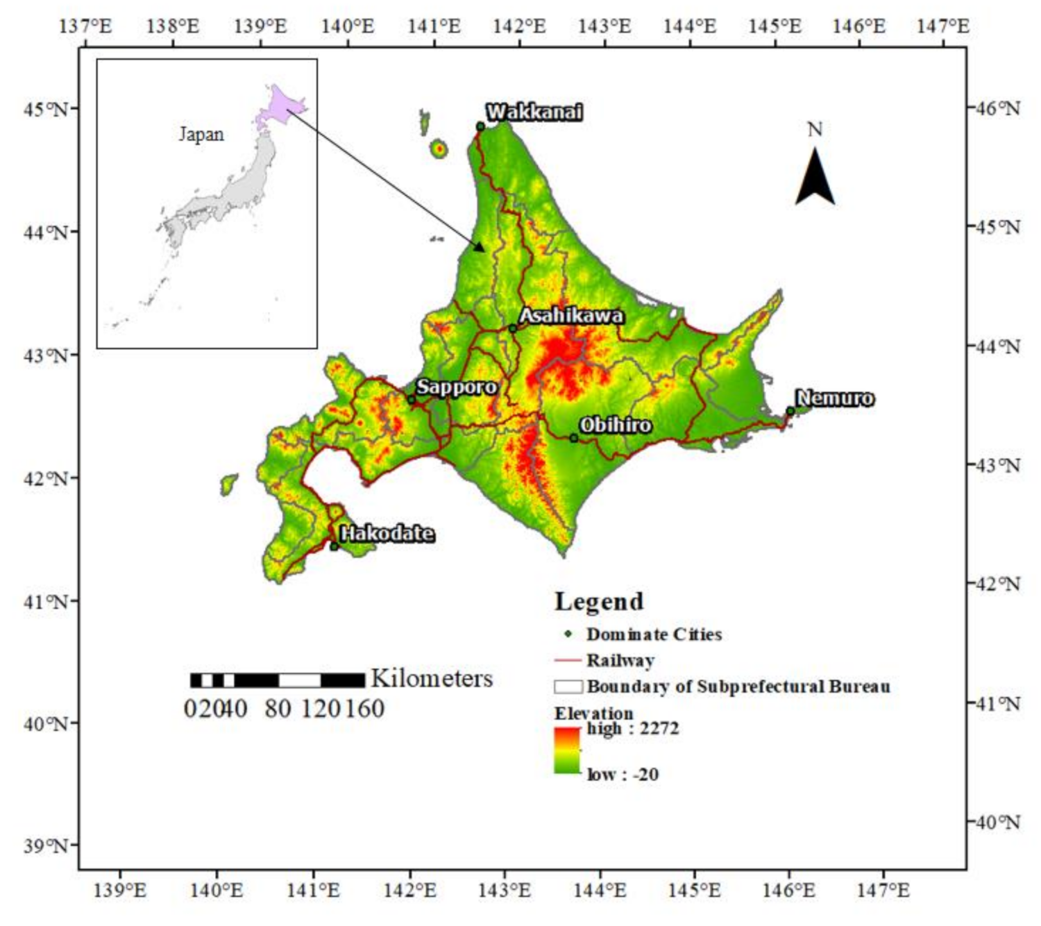
Hokkaido is located at the north of Japan (Figure 1), covering the area of about 8.3×10⁴ km² (excluding controversial territory). Geographically it lies in 40°33′N to 45°33′N and 139°20′E to 148°53′E. The elevation ranges from −20 m to 2272 m. Hokkaido is the only one administrative unit called “do” among 47 prefectures in Japan. In subunits, there are 14 subprefectural bureaus, which consist of 64 counties, 35 cities, 129 towns, and 15 villages. The terrain of Hokkaido is high in altitude in its center and relatively low in altitude at all sides near the coast. Mountainous areas account for 60% of the total land, and 40% of this area is occupied by volcanos.

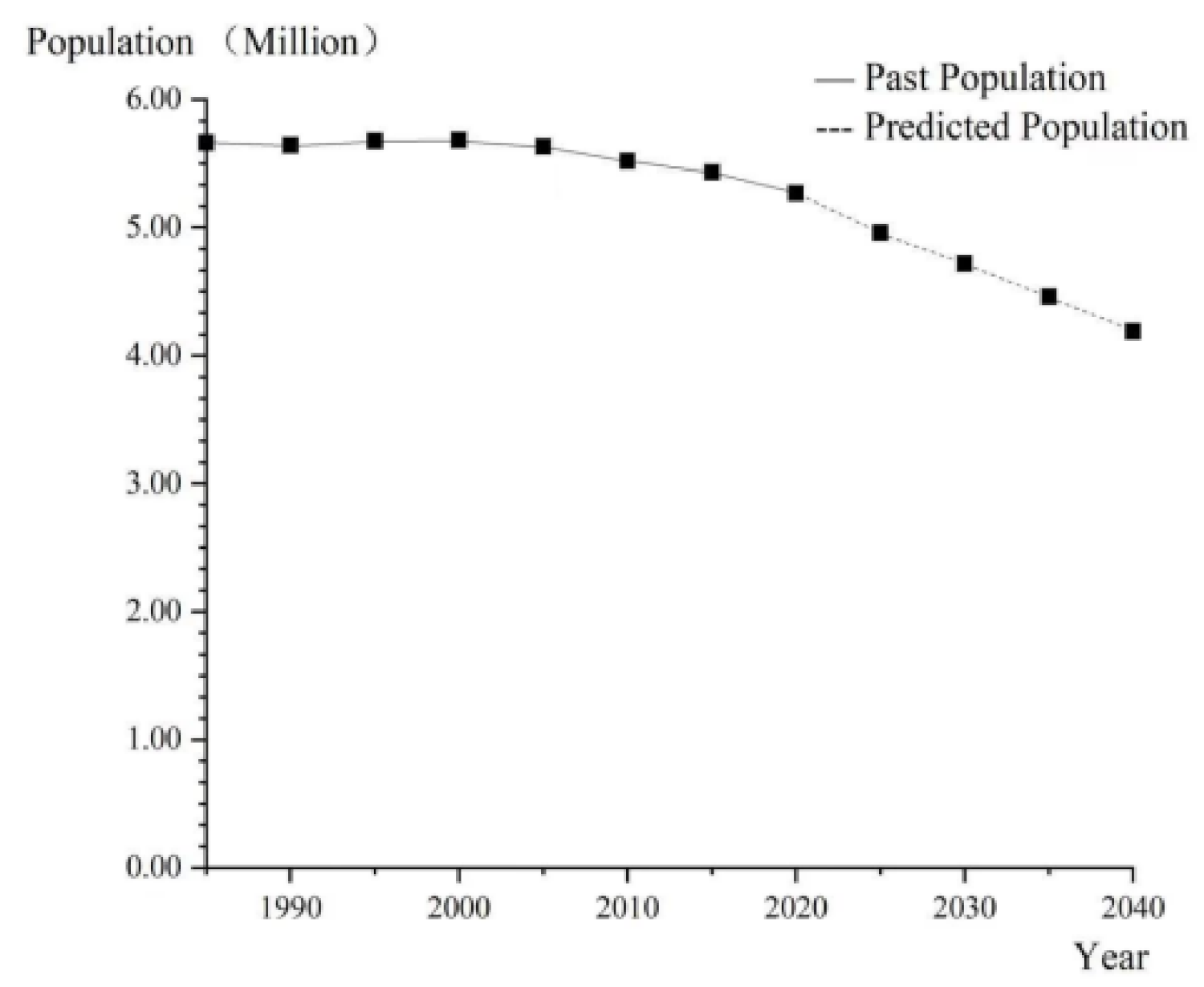
On January 1st in 2019, the population of Hokkaido was 5,268,352 and nearly half of is was living in Sapporo, the capital city of Hokkaido. The rest are mostly distributed in other central cities of subprefectural bureaus such as Hakodate, Obihiro and Asahikawa. The age structure of Hokkaido’s population is characterized by a serious old-aging trend. People over 65 years old account for nearly 40% of Hokkaido’s population.

Meanwhile, the negative natural growth rate of Hokkaido has led to a decreasing total population trend in recent years and future predictions (Hokkaido Population Vision, 2020). The National Institute of Population and Social Security Research (NIPSSR) conducted a population prediction showing the Hokkaido population is expected to drop by nearly 1/5 by 2040 (Figure 2).

Hokkaido is also one of Japan’s main forest lands, and its forests account for about 22% of Japan’s total forested area. The national forests of Hokkaido account for more than 50% of the total forest area of Hokkaido, including Mt. Daisetsu, the Hidaka Mountain and other major mountain ranges, creating one of the richest ecosystems in Hokkaido. The national forest of Hokkaido consists of conifers (Sakhalin fir and Sakhalin spruce) and broadleaf trees (Japanese oak, birch, and painted maple), whose views change with the seasons. The Hokkaido Regional Forest Office classifies national forests into four of five types depending on their main functions to conduct appropriate managements: water resource conservation type; landslide prevention type; recreational use type and nature conservation type [42].

Satellite images are downloaded from the United States Geological Survey (USGS) website at a resolution of 30 m, including Landsat Thematic Mapper (TM) data, Landsat Enhanced Thematic Mapper Plus (ETM+) data and Landsat Operational Land Imager (OLI) data. To reduce the missing information caused by snow cover, for each year, images in warm seasons (from 1 May to 31 October) were integrated at each pixel position over time by taking the median. Detailed information is shown in

Table 1. Landsat-based data used in the study.

Satellite	Sensor	Spatial Resolution (m)	Targeted Year	Origin
Landsat-5	TM	30	2010	USGS
Landsat-7	ETM+	30	2000	USGS
Landsat-8	OLI	30	2019	USGS

.

Considering the territory dispute between Japan and Russia regarding the boundaries of Hokkaido (the four northern islands), the administrative shape file in the disputed areas was excluded to fit the subsequent driving force analysis. Therefore, the Hokkaido vector files were not obtained from the Japanese government GSI but rather from the DIVA-GIS website (www.diva-gis.org (accessed on: 12 September 2020)) which removes the above disputed islands from Hokkaido domain.

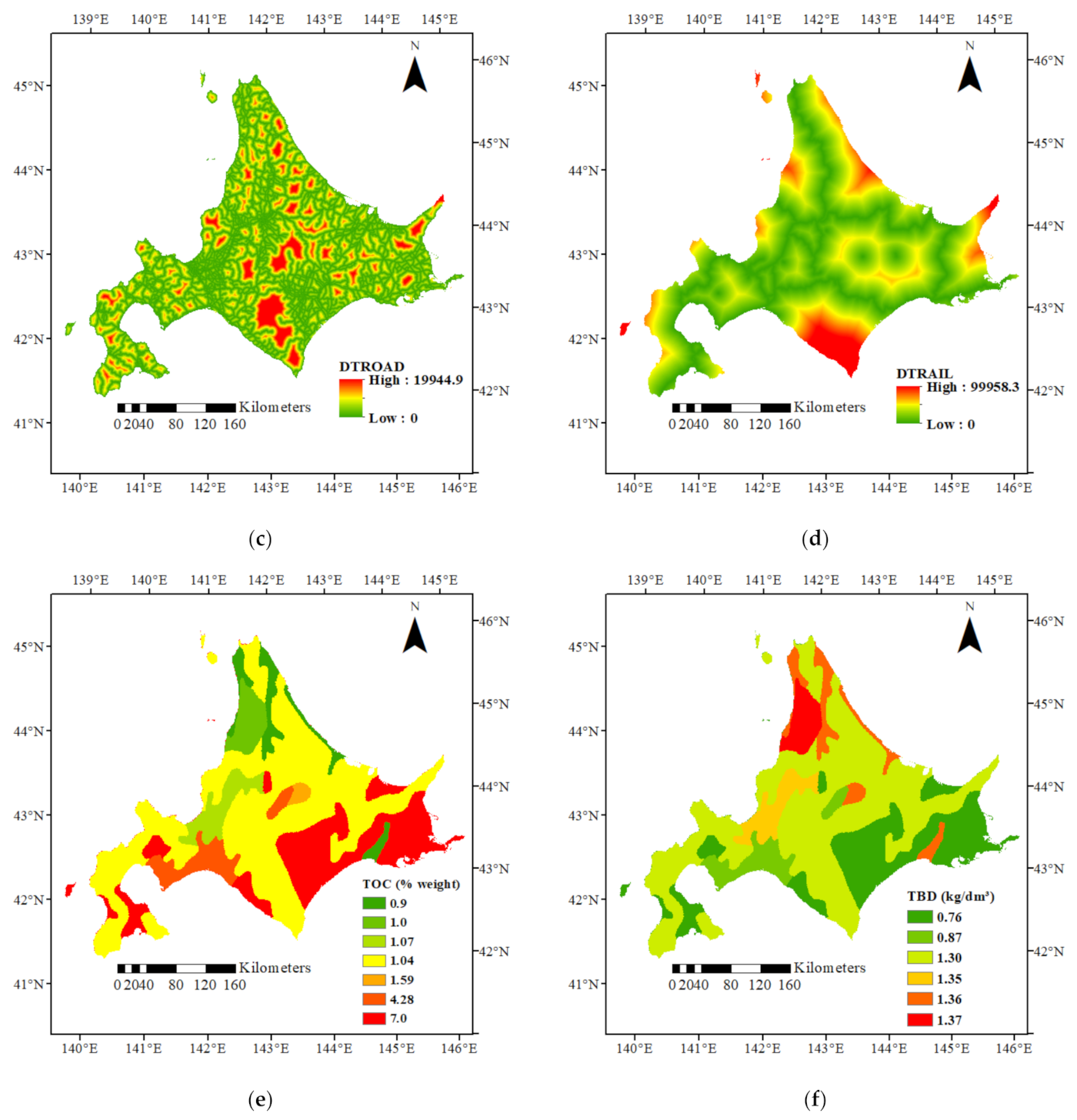
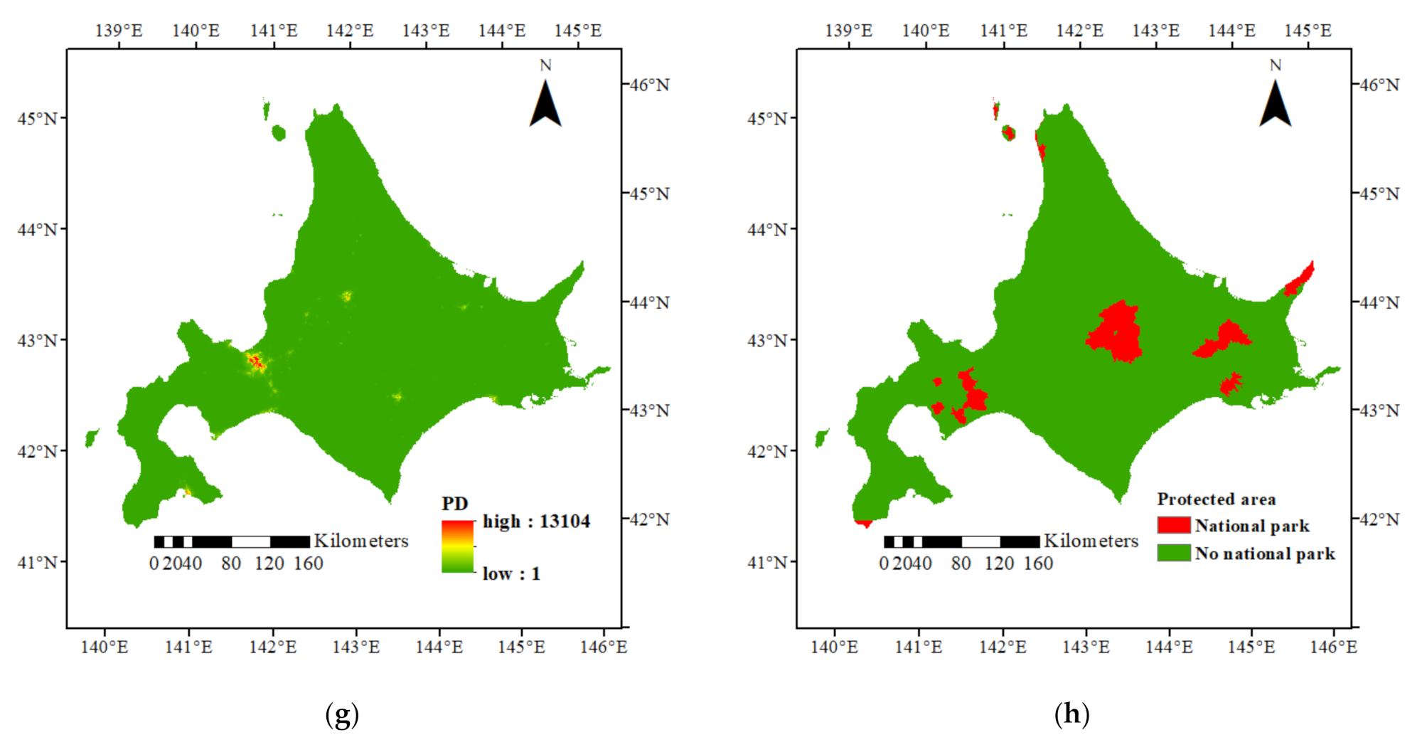
The change of land use is the result of the combined effect of natural factors and socio-economic factors, static and dynamic. Therefore, the selected factors should adhere to both natural factors and socio-economic factors to achieve a more accurate simulation of land use change. The selection of driving factors for land use change mainly conforms to the following four principles: (1) accessibility of factor data, which is a key issue for driving factor research and a guarantee for the accurate operation of related models; (2) consistency of factor data: The data should be consistent in time and space; (3) factor quantification, which can be input into the model, and simulation prediction can be realized; and (4) comprehensiveness of factor selection [43]. Based on this, seven land use change factors were selected, including digital elevation model (DEM), slope, distance to road (DTROAD), distance to railway (DTRAIL), organic carbon in topsoil (TOC), and bulk density in topsoil (TBD), population density (PD). In addition, a protected area of national parks from GSI are displayed as a policy refrain on land use change. The detailed descriptions of each factor are illustrated in

Table 2. Description of land use driver factors.

Factor	Units	Source
DEM	m	USGS
Slope	degree	USGS
DTROAD	Euclidean distance (m)	Open Street Map
DTRAIL	Euclidean distance (m)	Open Street Map
TOC	% Weight	Harmonized World Soil Database
TBD	kg/dm3	Harmonized World Soil Database
PD	/km2	WorldPop
Protected area	National parks	GSI

:

The administration-based masked raster files of land use driving factors were processed at unified resolution at 150 m due to the model calculator ability, as shown in Figure 3.

3. Methodology

This study includes two main processes: land use classification and future land use simulation. Figure 4 indicates detailed data input, computing methods (algorithm and models) and specific steps in each process.

3.1. Land Use Classification

Google Earth Engine (GEE) was used for processing image data. Landsat images are selected at Tiers 1 level, which has been treated systematically, geometrically, and topographically. The study site was mosaicked by clipping the Hokkaido boundary shape file in ArcGIS Pro 2.0 software. Sequentially, this study conducted radiometric and atmospheric correction in GEE and Pixel Information Expert Engine (PIE) (https://engine.piesat.cn/ (accessed on: 26 May 2021)) before classification step. By considering the land use situation of Hokkaido from GSI database, the types of land use were divided into six categories: cultivated land, forest, construction, grassland, waterbody, and others. The descriptions of each land use types are showed in

Table 3. Description of land use types.

Land Use Types	Description
Cultivated land	Arable land that is intended to plow and sow and raise crops for farming.
Forest	Land dominated by trees, including deciduous forest and evergreen forest
Waterbody	Rivers, lakes, ponds, wetlands.
Construction	Balconies, terraces (with or without roof), mezzanine floors and other detachable habitable areas.
Grassland	Grass, herb, and temporary meadows, including natural and artificial grass.
Others	Land covered by snow for long time and bare land in the top of mountains

.

The random forest (RF) classifier was employed in the supervised classification process of the GEE algorithm database to extract the above various land use classes. The RF algorithm can avoid errors such as data noise and over-fitting, which has great advantages for the classification of ground observation image data. Compared with the maximum likelihood method, single decision tree and single layer neural network method, the random forest algorithm is more successful in processing high-dimensional data and has higher accuracy [44].

The result of supervised classification depends heavily on the input training samples. To distinguish features under different conditions, the sample capacity of the initial training data set of the classifier needs to be large enough, especially in com-plex regions [45]. By visual observation on false-color composites (RGB) image to re-strict unchanging area in these three periods, totally 1695 points were selected in training sample set. A precise testing sample set is important for accuracy assessment of classifier and the quality of classification process [46]; hence, this study drew 1071 polygon-based testing samples by referring to the land use maps released by GSI. The number of samples for each land use is showed in

Table 4. Sample number of each land use type.

Land Use Type	Training (Points)	Testing (Polygons)
Cultivated land	198	202
Forest	580	254
Construction	117	180
Waterbody	23	70
Grassland	702	314
Others	75	51
Total	1695	1071

.

Five spectral features are applied to characterize typical land use categories, including normalized difference vegetation index (NDVI), normalized difference built-up index (NDBI), modified normalized difference water index (MNDWI), DEM and slope.

3.2. Land Use Simulation in 2040

3.2.1. Logistic Regression Analysis for Qualitative Analysis of Driving Factors

Because the FLUS model uses ANN to calculate the distribution probability of each land use type, it has good operability and explanatory properties. However, this method cannot intuitively reflect the positive or negative influences of driving factors on distribution probability of each land use. To reflect the qualitative impact of each driving factor on the distribution of land use, we used logistic regression analysis to calculate the regression constant of each driving factor on land use, thereby analyzing the positive or negative effects of each driving factor on each land type. After reclassing land use in 2019 into 6 single layers for each land use type, this study processed them with seven driving factor raster and its related autocorrelation factor raster into ASCII forms, and then computed results in Statistical Product and Service Solutions (SPSS, Version 25.0, IBM Corp, Armonk, NY, USA).

3.2.2. Autocorrelation Factor

A spatial autocorrelation factor is introduced as the input variable of the artificial neural network (ANN) model to detect the spatial autocorrelation effect to improve the simulation effect of the model. Spatial autocorrelation factors can be expressed as:

$$Autoco{v}_p=\frac{{\sum }_{p\ne j }{w}_{pj}{y}_j}{{\sum }_{p\ne j }{w}_{pj}}$$

(1)

where, Autocov_p is the spatial autocorrelation variable of a land use type on the cellular p; j is a neighborhood cell p; y_j indicates the occurrence of a class on the cell j (1 or 0); and w_pj is the spatial weight coefficient between cellular p and j. When the distance between p and j is less than threshold distance w_pj = 1; otherwise w_pj = 0.

3.2.3. Coupled Markov-FLUS Model

This study used a coupled Markov and future land use simulation (FLUS) model to dynamically simulate and predict land use/cover types in Hokkaido. Its construction principle is as follows: The cellular automata (CA) module based on the adaptive inertia mechanism in the FLUS model can only process spatial distribution by handling interaction between cells [34], while the Markov model can be used to predict the quantitative change of land use types. The Markov model cannot compute the changes in the spatial pattern [31].

The Markov model is a stochastic model used to predict the quantitative changes of land use, which dominates in its stability and no aftereffect. No aftereffect indicates that in a process of random development, the future state represented by t + 1 is only related to the current state represented by t. Stability refers to the stability of Markov’s process over a long period of time. Dynamic evaluation of land use/cover change features Markov’s stability and no aftereffect nature [47]. Therefore, it can be used to predict the changing trend of land use in the study area in the future. Its mathematical expression is shown below:

$${\mathrm{S}}_{\left(t+1\right)}={\mathrm{P}}_{ij}{\mathrm{S}}_{\left(t\right)}$$

(2)

where, S_(t+1) represents the state of land use type at t+1 time in the future; S_(t) represents the state of the land use type at the current time t; P_ij represents the state transition probability matrix of land use type.

The FLUS model is a tool for simulating future land use changes under both natural and social elements [48]. It combines an artificial neural network (ANN) algorithm, adaptive inertia, and competition mechanism to improve the traditional CA model, which is suitable for multi-scenario simulation. The back propagation neural network (BPNN) in the FLUS model is a multi-layer feedforward neural network [34]. Its basic composition includes an input layer, one or more hidden layers and an output layer, where the neurons of the input layer and the input the driving factors of land use change correspond to each other, and each neuron in the output layer corresponds to each type of land use. This model further combines the occurrence probability with converting cost, neighborhood effect and a self-adaptive inertia coefficient to estimate the combined probability of each land use grid, which can be relatively input in the panel of FLUS software. Among them, neighborhood effect ranges from 0 to 1, and a larger value indicates a stronger land expansion ability; inertia coefficient can be computed by CA evolution iterations; converting cost indicates the conversion difficulty from the current land use type to the target type, which is another factor shaping the land use dynamics.

4. Results

4.1. Land Use Classification Results

The land use change pattern in Hokkaido for three corresponding years are statistically and spatially illustrated in this section. The pixel-based data is resampled to 150 m resolution for the purpose of being compatible to model settings. The area of each land use and its changing trend are shown in

Table 5. Temporal land use distribution in area (km²) in Hokkaido.

Year	Cultivated Land	Forest	Waterbody	Construction	Grassland	Others
2000	8701.3	56,808.4	1374.1	1460.9	14,401.9	177.6
2010	7383.7	56,546.5	1268.1	1447.9	16,056.9	221.1
2019	8059.2	55,157.4	1419.4	1571.9	16,581.4	134.9

and Figure 5, respectively. The spatial land use distributions are disclosed in Figure 6.

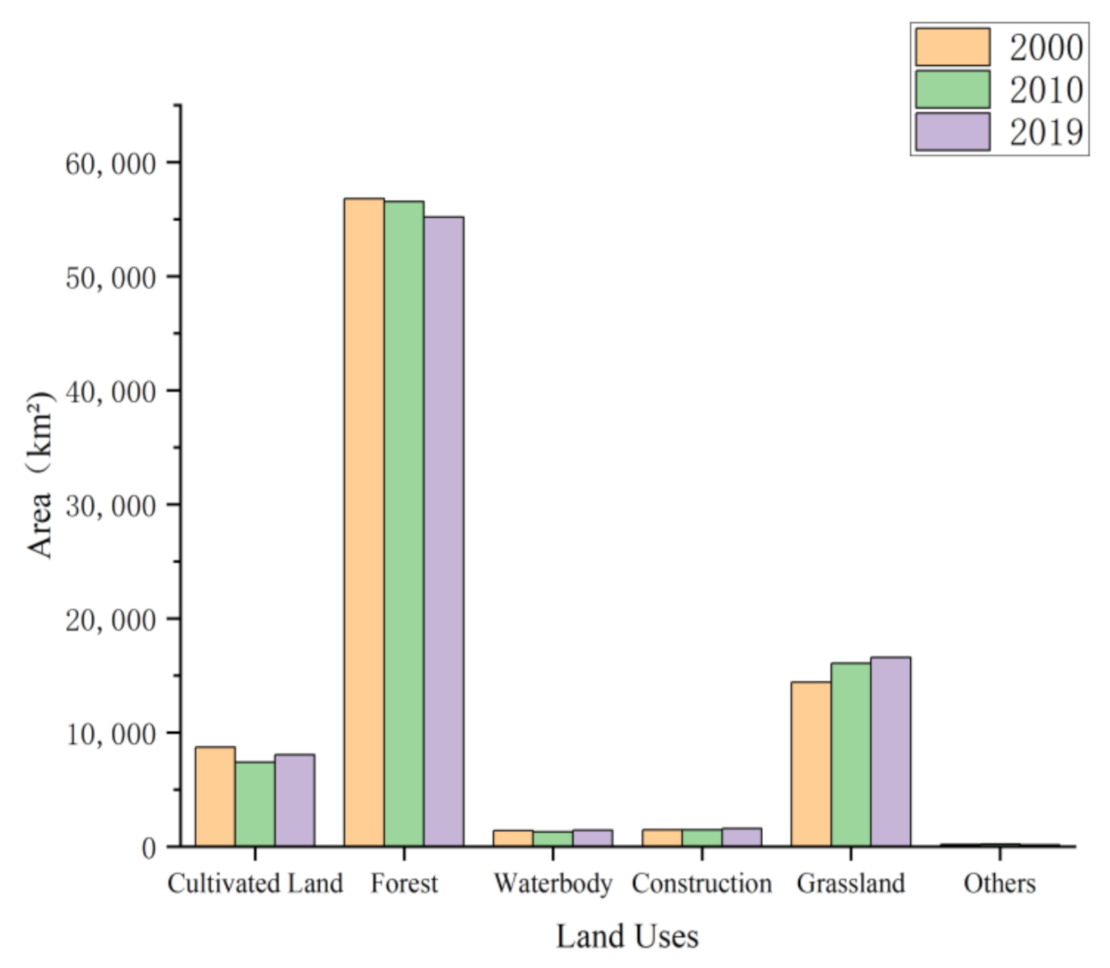
Regardless of the year, forest land in general accounts for the highest proportion of all types of land use in Hokkaido, followed by grassland and cultivated land. Forest land shows an overall downtrend from 2000, ending up at 55,157.4 km² in 2019. Grassland indicated an increasing trend, starting at 14,401.9 km² in 2000, rising to 16,581.4 km² in 2019. Cultivated land accounted 8701.3 km² in 2000, decreasing by 1317.6 km² in 2010, and eventually experienced an uptrend to 8059.2 km² in 2019. Construction area climbed slightly to 1571.9 km² in 2019 from 1460.9 km² in 2000.

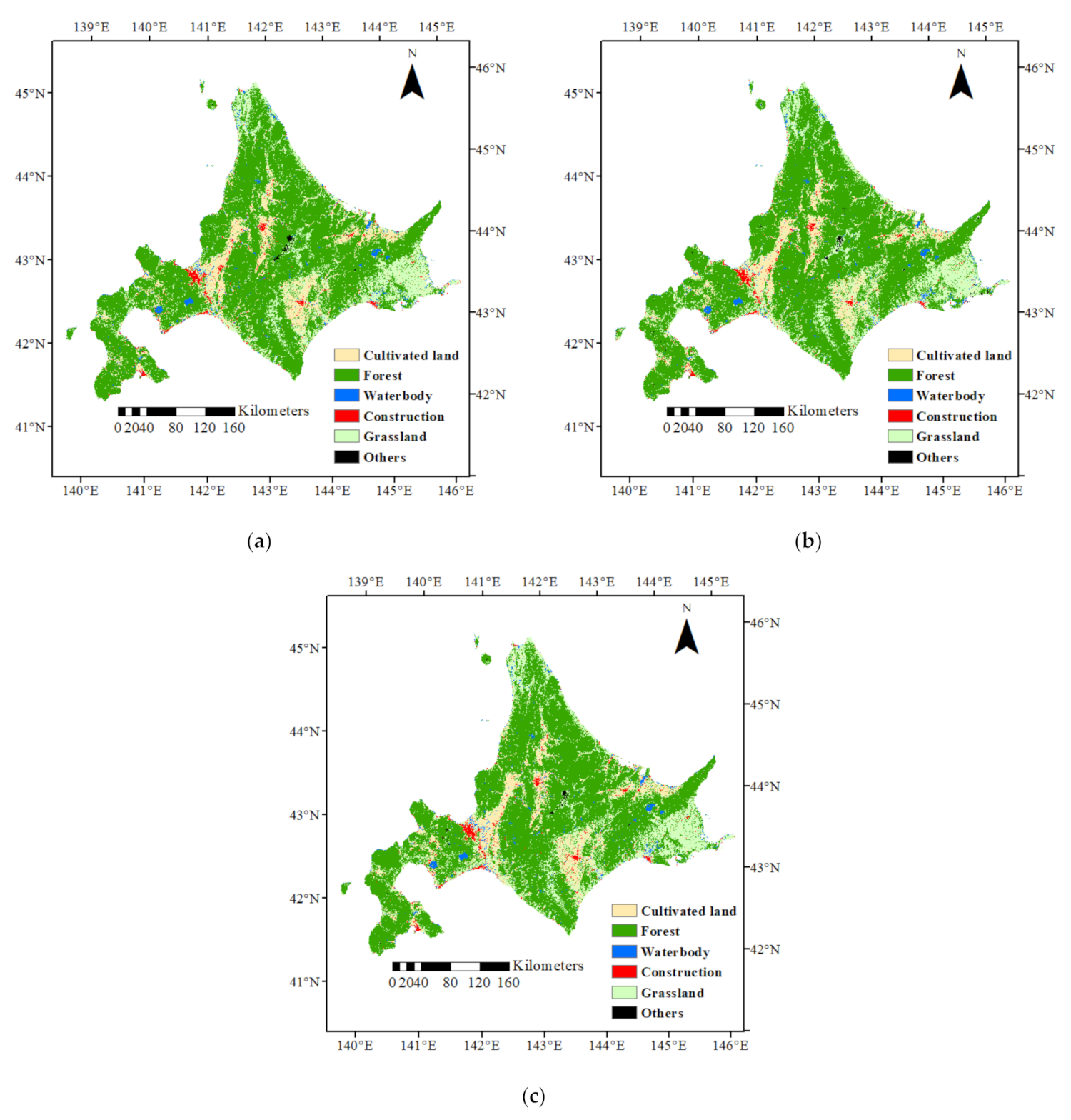
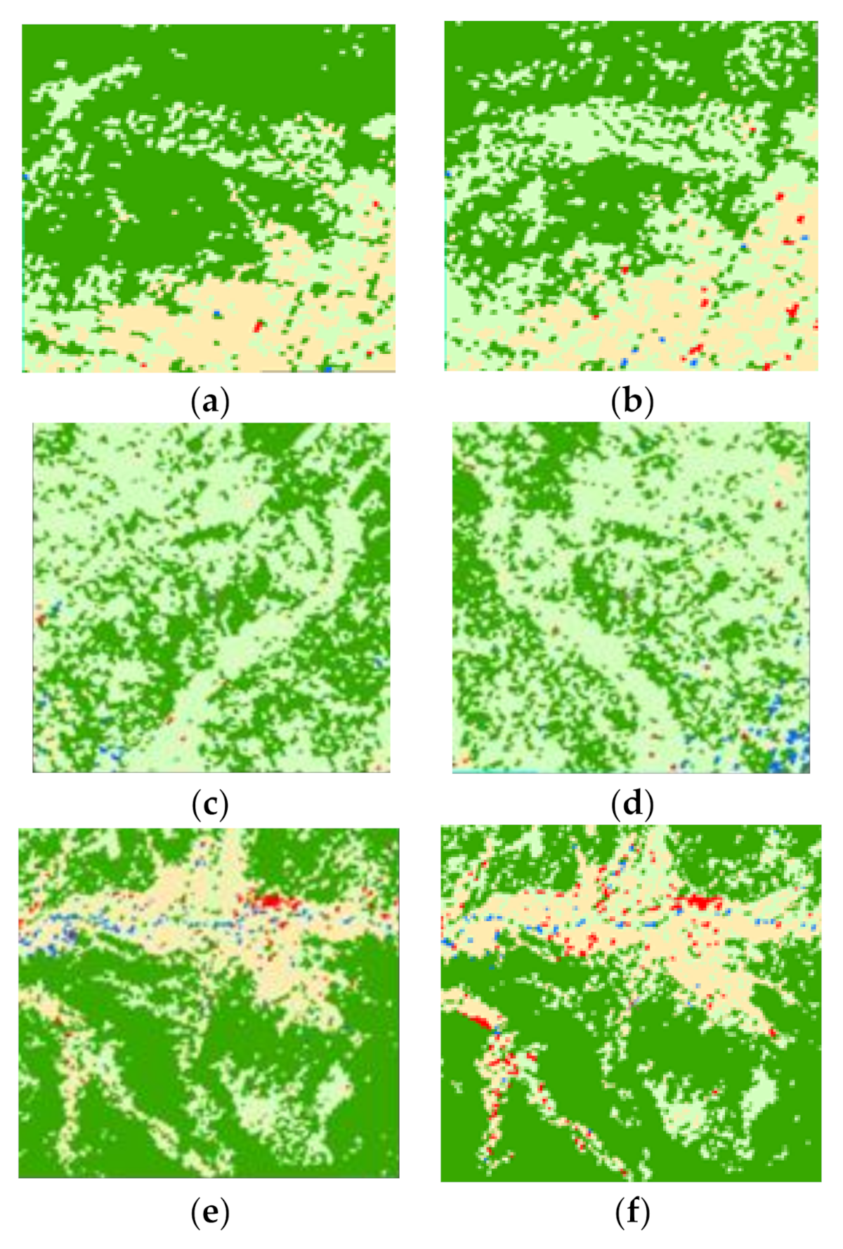
As the indication of Figure 6, spatial change of land use in Hokkaido has not been significant during this period. Cultivated land is mainly located in areas dominated by plains, mainly in the center and southeast of Hokkaido. Except for some sporadic distribution the in southern and central parts of Hokkaido, grasslands are mainly distributed in the west of Hokkaido. During this period, part of the grassland and cultivated land expanded to forest, especially in the north of the Tokachi subprefectural Bureau and the west of Nemuro subprefectural Bureau. However, some cultivated land in Hiyama subprefectural Bureau has been converted into grassland and construction. Figure 7 shows some examples of distributed change between 2000 and 2019.

The land use transition matrix is used to describe the mutual change of various land use types, and mainly reflects the dynamic model of the mutual quantity transition of various types at different time points. Hokkaido land use transition matrix in the periods 2000 to 2010 and 2010 to 2019 are shown in

Table 6. Land use transition matrix in area (km²) (2000 to 2010).

2000/2010	Cultivated Land	Forest	Waterbody	Construction	Grassland	Others	Total
Cultivated land	5446.8	466.5	118.8	328.3	1021.2	2.1	7383.7
Forest	528.0	53,239.2	91.7	15.3	2649.7	22.6	56,546.5
Waterbody	87.1	112.5	876.1	20.7	170.7	1.1	1268.1
Construction	318.8	29.5	26.6	974.8	97.1	1.1	1447.9
Grassland	2315.0	2893.2	257.2	118.9	10,401.8	70.9	16,056.9
Others	5.8	67.5	3.7	2.9	61.4	79.8	221.1
Total	8701.3	56,808.4	1374.1	1460.9	14,401.9	177.6	82,924.2

and

Table 7. Land use transition matrix in area (km²) (2010 to 2019).

2010/2019	Cultivated Land	Forest	Waterbody	Construction	Grassland	Others	Total
Cultivated land	5155.0	497.3	88.0	317.1	1999.4	2.4	8059.2
Forest	330.8	52,054.3	93.9	15.0	2588.1	75.3	55,157.4
Waterbody	188.7	135.6	856.7	26.6	208.2	3.7	1419.4
Construction	394.4	39.3	32.0	987.6	115.6	3.0	1571.9
Grassland	1313.1	3787.3	196.4	100.4	11,118.9	65.3	16,581.4
Others	1.7	32.7	1.1	1.2	26.8	71.3	134.9
Total	7383.7	56,546.5	1268.1	1447.9	16,056.9	221.1	82,924.2

, respectively. The values shown in bold font indicate no change in land use type for the given period.

Table 8. Accuracy assessment for land use classification.

	2000		2010		2019
	UA (%)	PA (%)	UA (%)	PA (%)	UA (%)	PA (%)
Cultivated land	96	81	96	72	96	73
Forest	91	98	92	98	90	96
Waterbody	95	99	97	99	91	99
Construction	87	94	84	94	82	94
Grassland	83	87	74	89	77	86
Others	67	64	59	61	58	69
OA (%)	90		88		88
Kappa	0.87		0.84		0.84

present the accuracy assessment results of Hokkaido obtained from RF algorithm with user’s accuracy (UA), producer’s accuracy (PA), overall accuracy (OA) and Kappa value. Training points for accuracy assessment adopted stratified random sampling method, which depends on the proportional area of each class; therefore, land types with small area easily tend to get the lower accuracy. However, the overall accuracy for all the LULC classification maps exceeded 88%.

4.2. Land Use Simulation Results

4.2.1. Qualitative Analysis for Driving Factors

Table 9. Logistic regression results for land use driving factors.

Regression Coefficients	Cultivated Land	Forest	Waterbody	Construction	Grassland	Others
DEM	0.000316	−0.000376	0.000871	−0.000457	0.00047	−
Slope	−0.008638	0.012464	−0.011263	0.004122	−0.005547	0.008596
DTROAD	−0.000531	0.000353	−0.000129	−0.001422	0.000177	0.000855
DTRAIL	−0.000008	0.000002	−0.000024	−0.000051	−0.000088	−0.000378
TOC	0.001158	−0.001131	0.000082	0.001035	0.00022	−
TBD	0.005384	−0.010975	−	0.002957	−	−
PD	−0.000064	0.00003	−	−	0.00018	−0.000586
Constant	0.161217	1.662243	1.736424	0.266319	0.21557	1.795446
ROC	0.881	0.798	0.999	0.986	0.976	0.951

reflects the regression results of regression constants, regression coefficients between land use distribution and driving factors, and ROC value for each group.

From the regression results, soil quality TOC and TBD have a positive impact on the distribution of cultivated land, while DTROAD, DTRAIL and slope influence the distribution negatively. This is consistent with a previous study [49]. Forests can be more dramatically affected by slope. DTROAD and DTRAIL shows as negative drivers targeted to upbringing of waterbody and construction. However, it is showed that distribution of forest and DTRAIL have positive relationship, which may be due to the special topography trait of Hokkaido. In general, it is believed that the ROC value greater than 0.7 can indicate a reliable simulation result; therefore, this study can better explain the effects of land use driving factors with all ROCs over 79%.

4.2.2. Accuracy Assessment for Land Use Simulation

By importing the current land use data in 2010 in the CA module of the FLUS software, based on the occurrence probability map computed by inputting driving factors to ANN with and without autocorrelation variables, two 2019 land use simulation maps are generated for accuracy comparison. The setting parameters include the number of iterations 300; the size of the neighborhood 3; the model acceleration factor 1, and the simulated land quantity to the actual land use quantity in 2019. The optimal land-type transformation rules are shown as

Table 10. Optimal land-type transformation rules.

	Cultivated Land	Forest	Waterbody	Construction	Grassland	Others
Cultivated land	1	1	1	1	1	1
Forest	1	1	1	1	1	1
Waterbody	0	0	1	0	0	0
Construction	0	0	0	1	0	0
Grassland	1	1	1	1	1	1
Others	1	1	1	1	1	1

, where 0 means that it cannot be changed, and 1 means that it can be changed. This study mainly compared the overall accuracy (OA) under two different conditions, we found after inducing autocorrelation factor, the OA of simulation climb slightly from 0.831 to 0.834 and Kappa value increased from 0.665 to 0.671, therefore, we will apply this factor into simulation process in subsequent steps.

4.2.3. Scenario-Based Future Land Use Prediction

In natural development (ND) scenario, land type transformation rules in Table 10 have been applied in process. The national park is added as a restricted area, and the natural evolution forecast area based on Markov estimation in

Table 11. Markov estimation of future land use demand (Unit: number of pixels).

Year	Cultivated Land	Forest	Waterbody	Construction	Grassland	Others
2030	277,954	2,515,995	51,968	59,843	768,193	11,567
2040	267,204	2,521,686	50,919	57,678	776,127	11,906

is used as the land use demand area for 2040.

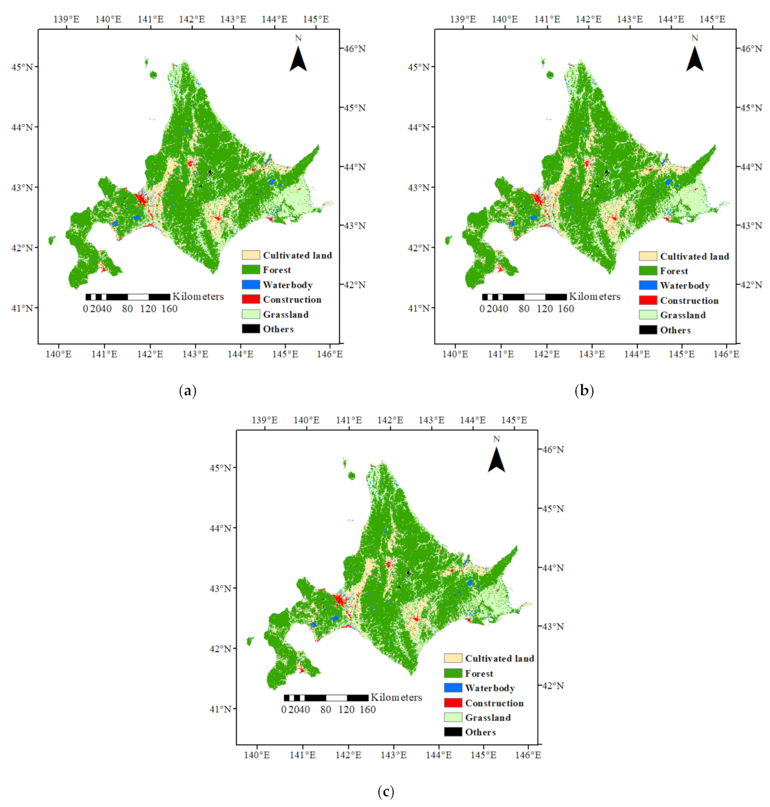
Considering that the area of cultivated land under the ND scenario has been reduced to a certain extent, this study constructed a CP scenario by restraining this change. CP scenario is based on ND scenario, while it defines area of cultivated land in 2019 as a protected area which is added into restricted area. Similarly, FP scenario is based on ND scenario, while it defines forest area in 2019 as a protected area which is added into restricted area. The land use distributions under the three scenarios are shown in Figure 8.

5. Discussion

5.1. Past-to-Future Land Use Pattern (2000–2040)

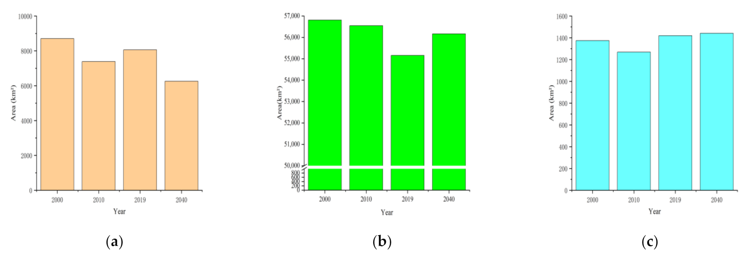
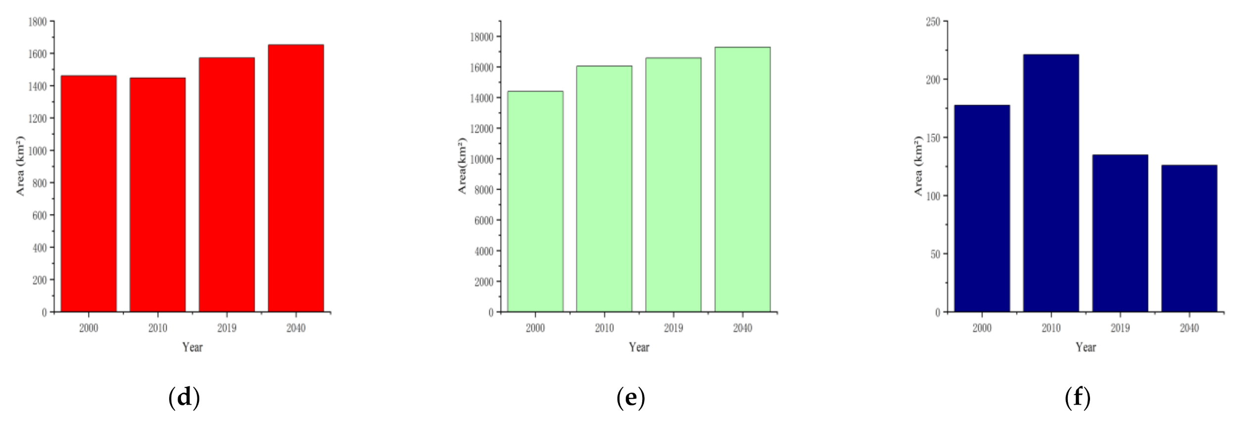
Figure 9 indicates area changes of 6 land use classes in Hokkaido from 2000 to 2040. The period between 2000 and 2019 is based on the classification results, and the amounts in 2040 are derived from simulation results in ND scenario.

The results of this study show that Hokkaido has had a significant decline in cultivated land in the past and will the decline will continue in the next 20 years, while the area of grassland will have a clear upward trend. This shows that during the period, the abandonment of cultivated land will become more serious. According to the simulation analysis based on the driving factor, the abandoned farmland will be converted into grassland (in this case, abandoned area) to a large extent, and part of it will be occupied by construction, which is consistent with the trend reflected in both Table 6 and Table 7 and Figure 9.

The abandonment of farmland in Hokkaido has become an issue affecting the sustainability of land use since the last 1980s [50], which is a direct reflection of the future reduction of cultivated land in Hokkaido. Previous studies have shown that the main factors for the abandonment of farmland in Hokkaido include natural and social factors: natural factors consist of geographic location, slope and elevation, soil quality, while social factors mainly include policy and demographic changes. It is worth mentioning that the impact of policies on farmland abandonment can be two contrast ways. For instance, the “Hokkaido Comprehensive Development Plan (HCDP)” aims to promote the relocation, concentration, and intensification of farmland, and to increase agricultural productivity and farmers’ income [49], which encourages to abandoned barren and hard-to-use farmland. However, the “Direct Payment (DP) system” in Hokkaido slowed down the growth rate of abandoned farmland through financial subsidies to farmers [51]. Therefore, to maximize the sustainability of cultivated land use in Hokkaido, this study did not simulate the impact of certain policies. Instead, it directs the effects that policy can make, that is, to minimize the abandonment of cultivated land to construct CP scenario.

The demographic changes in Hokkaido will also have an impact on the abandonment of farmland. The results of logistic regression analysis in this study show that population density and the distribution of cultivated land are negatively correlated, which means that the more concentrated the population is in urban areas, the lower the probability of cultivated land. According to the government’s employment statistics (www.pref.hokkaido.lg.jp (accessed on: 15 December 2020)) from 2000 to 2019, the proportion of people engaged in farming in Hokkaido has decreased and the number of farmers over 65 years old has consistently risen, while the urbanized population is increasing, and it can be claimed that the increase of urban population will promote the expansion of the urban construction [52,53,54]. This is consistent with the results of the decrease of cultivated land in Figure 8a and the increase of construction in Figure 8e.

Compared with the area changes of other land use types, waterbody and others did not change significantly from 2000 to 2019 and are not estimated to change much in the future. For waterbody, the changes in this stage are likely to be caused by the classification error of the cultivated land, especially in areas with paddy fields, which occurs frequently in the Ishikari Plain. As far as others, the main reason for its low accuracy is the uncertainty of snow distribution on the surface. Except for some high-altitude mountains, most of the snow-covered areas have a great relationship with the climatic conditions of the target year.

5.2. Comparison of Scenario-Based Land Use Situations

As the area of cultivated land in Hokkaido has a clear downward trend in the context of natural development (ND), This study achieves the sustainable use of cultivated land by restricting the transfer of cultivated land to other land (

Table 12. Comparison of land use area (km²) between ND, CP, and FP scenarios in 2040.

Scenario/Land Use	Cultivated Land	Forest	Waterbody	Construction	Grassland	Others
Natural Development	6012.1	56,225.8	1442.3	1653.3	17,463.7	126.9
Cultivated land Protection	8013.9	54,918.5	1433.1	1590.8	16,841.0	126.9
Forest Protection	6011.9	56,738.2	1439.1	1650.5	16,958.5	126.0

). The area of cultivated land obtained in ND scenario is compared with the CP scenario and the FP scenario, respectively. An increase of about 25% in cultivated land in CP scenario indicates that the policy of protecting cultivated land can effectively improve the sustainable use of cultivated land. In addition, the amount and spatial distribution of cultivated land use in 2019 are almost the same as in the CP scenario, which shows that the demand for cultivated land in Hokkaido has been basically saturated, and it may only remain unchanged or decrease in the future.

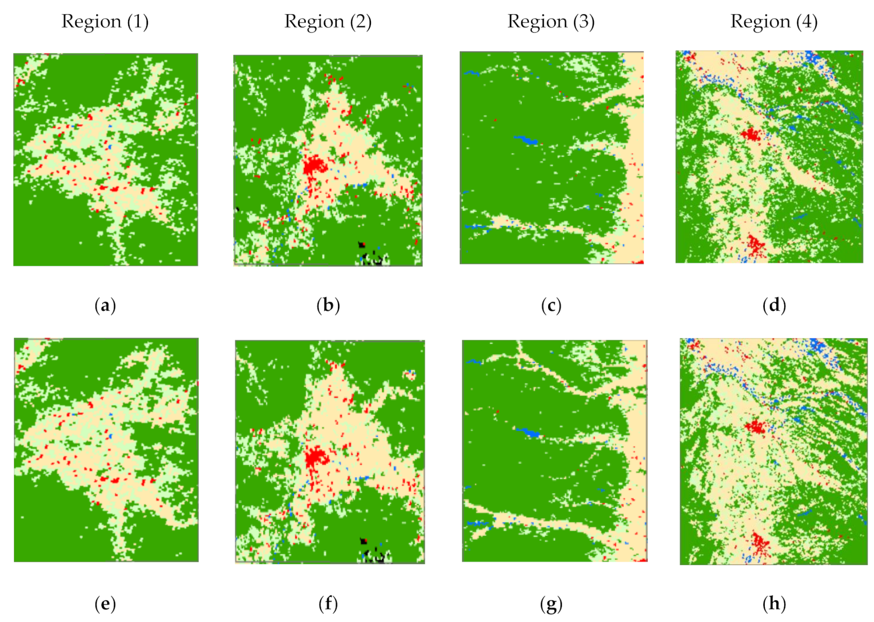
By comparing the ND scenario and the CP scenario, we can summarize the spatial change trends of the cultivated land in the two scenarios in the future, mainly showing the following three points. Firstly, in the ND scenario, the cultivated land is more likely to be converted into forest, grassland, or construction due to the concentration of agriculture. This includes the expansion of forest land from the center to the surrounding area and the increase of scattered buildings (

Table 13. Land use transition matrix in area (km²) (2019 to 2040 (ND scenario)).

2019/2040 (ND)	Cultivated Land	Forest	Waterbody	Construction	Grassland	Others	Total
Cultivated land	5569.3	151.2	0.0	0.0	291.6	0.0	6012.1
Forest	1312.3	53,300.5	0.0	0.0	1606.8	6.3	56,225.8
Waterbody	17.1	2.8	1419.4	0.0	3.1	0.0	1442.3
Construction	62.0	3.5	0.0	1571.9	16.0	0.0	1653.3
Grassland	1098.6	1699.3	0.0	0.0	14,663.9	1.9	17,463.7
Others	0.0	0.3	0.0	0.0	0.0	126.6	126.9
Total	8059.2	55,157.4	1419.4	1571.9	16,581.4	134.9	82,924.2

and Figure 10a,e and Figure 10b,f). Secondly in CP scenario, the cultivated land at the edge location has been effectively protected, resulting in a slowdown in the rate of cultivated land abandonment (Figure 10c,g). (3) Grassland tends to be transformed into forest land under the ND scenario and be transformed into cultivated land or maintained under the CP scenario (Figure 10d,h).

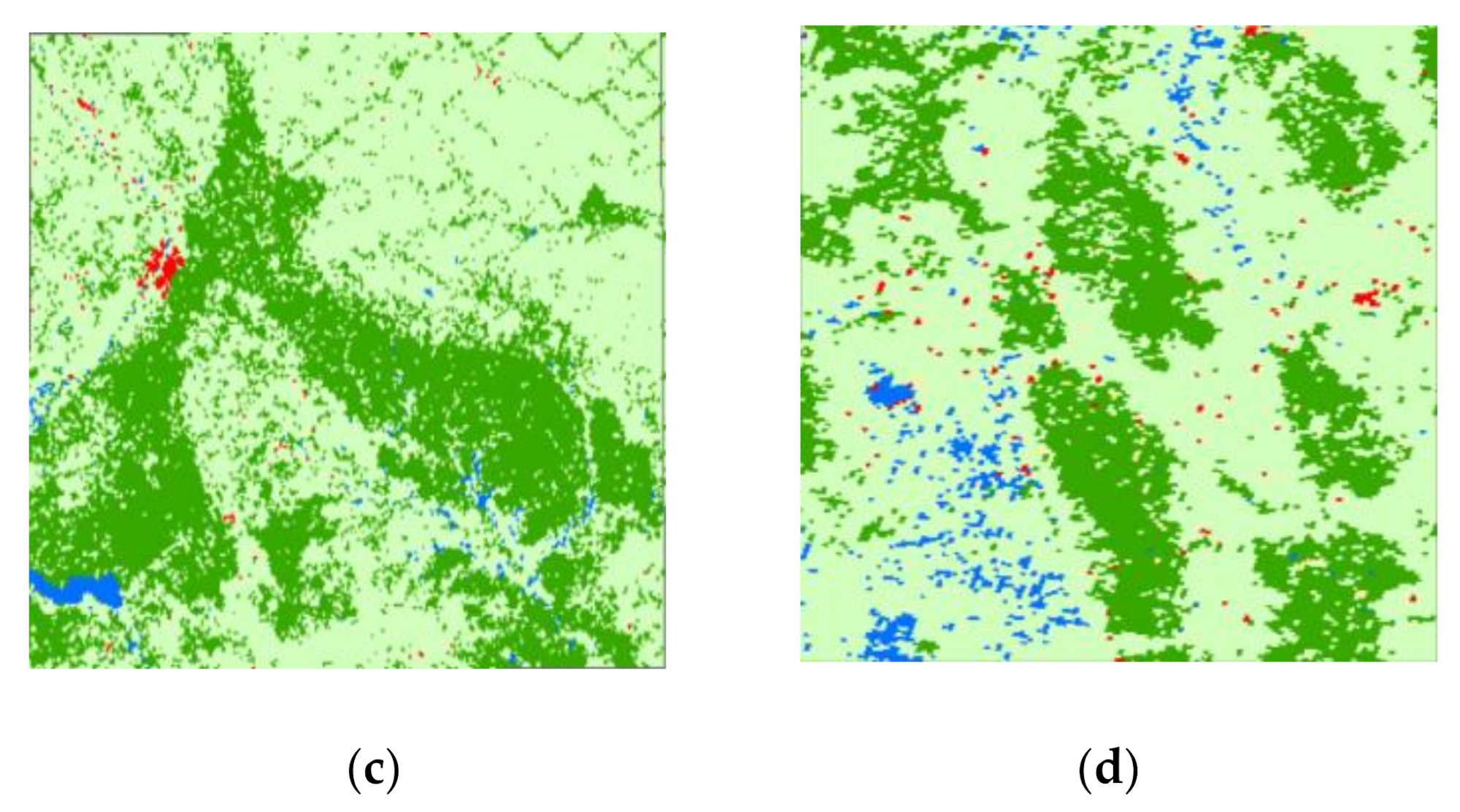
Due to the important position of forest land on Hokkaido, this study explored the possible changes of forest land in the future by constructing FP protection scenarios. In CP scenario, a reduction of 1310 km² was found in the forest compared to the ND scenario (Figure 11), while in FP scenario, the forest has increased by 509.7 km² compared to the ND scenario (Figure 12). The increase in forest land is mainly due to the conversion from abandoned farmland and the slowing down of grassland expansion, especially in mass graze-based grassland in east of Hokkaido (Figure 13a,c and Figure 13b,d).

5.3. Recommendations and Suggestions

Based on the comparative analysis of the characteristics of land use evolution, existing problems, and multi-scenario simulation results in this study, the following suggestions are put forward for the optimization and adjustment of future land use in Hokkaido: (1) Our results show that restricting land use areas can effectively enhance the sustainable use of cultivated land. Therefore, it is advisable to strengthen the protection of cultivated land, by regulating a basic cultivated land protection system and compensation system (such as Direct Payment) should be established to ensure the balance of cultivated land occupation and its quality. (2) Promote the transformation of government functions by strengthening land regulation and supervision, meanwhile restrict the trading of private cultivated land in Hokkaido. Public funds should be used to restore the use of abandoned arable land, and at the same time, through agricultural technology, to ensure that Hokkaido’s food production continues to meet the minimum standards of national food security. (3) The results show a mass area of grassland replacing cultivated land in the future. Hence, by centralizing grazing activities, the expansion of Hokkaido’s grassland into cultivated land and forest can be effectively restrained, especially at the boundaries between grassland and these lands. Simultaneously, the unused grassland converted from abandoned farmland should be conserved to ensure that its fertility is capable of being converted back into cultivated land in the future. (4) From the regression results, this study concludes intensive population in urban area is not beneficial to the development of cultivated land. Consequently, controlling the concentration of population in Hokkaido cities and encouraging people to relocate to the non-central areas is necessary for cultivated land protection. By improving transportation, medical care, education and other functions, the population distribution of Hokkaido can be dispersed.

The fifth basic land use plan (www.pref.hokkaido.lg.jp (accessed on: 22 May 2021)) of Hokkaido stipulates that the cultivated land in the basic farming area cannot be used for other purposes, which fits well with recommendations 1 and 2. The existing farmland will be protected to the maximum extent, and the fertile but abandoned cultivated land will be protected and appropriately improved. For cultivated land in non-agricultural areas, where adjustments are expected to conduct non-agricultural land use planning (such as urban planning), stakeholders will follow the adjusted planning older which is used to define the “Good Cultivated Land” or not, and this “Good Cultivated Land” will be properly preserved. However, the criteria for formulating this order are multifaceted, not only related to the land itself, but also to its geographic location and the attitude of the owner, which complicates the protection of cultivated land outside of agricultural areas. Policymakers are supposed to clearly define what is “Good Cultivated Land” but not depend on an obscure consultation with landlord.

5.4. Limitations and Future Works

In general, some shortcomings of the study can be concluded based on the following four points:

(1) The remote sensing data for making land use classification are at a resolution of 30 m and the simulation process is at a resolution of 150 m, which indicates there are still some details requiring more accurate interpretation. (2) The classifications of cultivated and waterbody, cultivated land and grassland without considering the phenological law, are more likely to be confused. Moreover, due to the large area of Hokkaido, it is difficult to collect training sample sets based on field surveys, resulting in certain classification errors. (3) Driving factors have relatively limited impact on land use, and different types of driving factor weights cannot be assigned, that is, the influence weights of factors on land use cannot be grasped well. (4) Moreover, scenarios differ from absolute restricted area, but the actual situation is hard to develop towards these directions.

Accordingly, further studies are supposed to include the below solutions: (1) use of relatively high resolution satellite data to optimize land use classification process if it is technically and economically feasible; (2) to investigate the phenological laws of various vegetation types, especially paddy rice in cultivated land, for improving the classification accuracy; (3) to use appropriate weight analysis methods to rank the influence of land use driving factors; (4) to collect policy documents to support the establishment of target future land use scenarios.

6. Conclusions

This research used remote sensing classification methods based on a random forest algorithm to monitor the spatiotemporal changes in six land classes (cultivated land, forest, waterbody, construction, grassland, and others) on Hokkaido from 2000 to 2019, with an overall accuracy of classification over 88%. Based on the analysis of land use changes and driving factors including DEM, slope, PD, DTRAIL, DTROAD, TOC, TBD and autocorrelation factors added to improve simulation accuracy, the coupled Markov-FLUS model is applied by changing the restricted area to simulate spatial distributions of land use in natural development scenario, cultivated land protection scenario, and forest protection situation of Hokkaido in 2040. The land use classification results show from the period of 2000 to 2019, the area of cultivated land in Hokkaido shows a downward trend with a reduction of 642.1 km², while construction has increased by 111.0 km² and grassland expanded by 2179.4 km², while the forest and waterbody areas have not changed significantly. The simulation results of future land use changes show that under the natural development scenario, the cultivated land in Hokkaido will be reduced by about 25% by 2040, and the reduced cultivated land is more likely to be converted into grassland and forest land. In the cultivated land protection scenario, the area of cultivated land remains basically unchanged, which shows that the use of cultivated land in Hokkaido has reached saturation, and about 239.0 km² forest land will be invaded by other land types. In forest protection scenario, the area of forest in Hokkaido will increased by around 1580.8 km², but the change trend of cultivated land is following natural development scenario. Grassland, especially in mass intensive graze-based area of eastern Hokkaido, will have an obvious expansion trend. This study provides a reference for future land use planning and management in Hokkaido, and it is expected to support the sustainable land use development with different targets.

References

- An, H.; Wu, X.; Zhang, Y.; Tang, Z. Effects of land-use change on soil inorganic carbon: A meta-analysis. Geoderma 2019, 353, 273–282. [Google Scholar] [CrossRef]
- Liang, X.; Guan, Q.; Clarke, K.C.; Liu, S.; Wang, B.; Yao, Y. Understanding the drivers of sustainable land expansion using a patch-generating land use simulation (PLUS) model: A case study in Wuhan, China. Comput. Environ. Urban Syst. 2021, 85, 101569. [Google Scholar] [CrossRef]
- Deng, Z.; Zhang, X.; Li, D.; Pan, G. Simulation of land use/land cover change and its effects on the hydrological characteristics of the upper reaches of the Hanjiang Basin. Environ. Earth Sci. 2015, 73, 1119–1132. [Google Scholar] [CrossRef]
- Huang, M.; Chen, N.; Du, W.; Chen, Z.; Gong, J. DMBLC: An Indirect Urban Impervious Surface Area Extraction Approach by Detecting and Masking Background Land Cover on Google Earth Image. Remote Sens. 2018, 10, 766. [Google Scholar] [CrossRef] [Green Version]
- Shao, Z.; Ding, L.; Li, D.; Altan, O.; Huq, E.; Li, C. Exploring the Relationship between Urbanization and Ecological Environment Using Remote Sensing Images and Statistical Data: A Case Study in the Yangtze River Delta, China. Sustainability 2020, 12, 5620. [Google Scholar] [CrossRef]
- El-Kawy, O.A.; Rød, J.K.; Ismail, H.; Suliman, A. Land use and land cover change detection in the western Nile delta of Egypt using remote sensing data. Appl. Geogr. 2011, 31, 483–494. [Google Scholar] [CrossRef]
- Huq, E.; Rahman, M.; Al Mamun, A.; Rana, M.P.; Al Dughairi, A.A.; Longg, X.; Javed, A.; Saleem, N.; Sarker, N.I.; Hossain, M.A.; et al. Assessing vulnerability for inhabitants of Dhaka City considering flood-hazard exposure. Geofizika 2020, 37, 97–130. [Google Scholar] [CrossRef]
- Gao, J.; Zha, Y. Assessment of the effectiveness of desertification rehabilitation measures in Yulin, north-western China using remote sensing. Int. J. Remote Sens. 2001, 22, 3783–3795. [Google Scholar] [CrossRef]
- Dong, J.; Xiao, X.; Menarguez, M.A.; Zhang, G.; Qin, Y.; Thau, D.; Biradar, C.; Moore, B. Mapping paddy rice planting area in northeastern Asia with Landsat 8 images, phenology-based algorithm and Google Earth Engine. Remote Sens. Environ. 2016, 185, 142–154. [Google Scholar] [CrossRef] [Green Version]
- He, Y.; Lee, E.; Warner, T.A. A time series of annual land use and land cover maps of China from 1982 to 2013 generated using AVHRR GIMMS NDVI3g data. Remote Sens. Environ. 2017, 199, 201–217. [Google Scholar] [CrossRef]
- Phiri, D.; Morgenroth, J. Developments in Landsat Land Cover Classification Methods: A Review. Remote Sens. 2017, 9, 967. [Google Scholar] [CrossRef] [Green Version]
- Zhang, H.K.; Roy, D.P. Using the 500 m MODIS land cover product to derive a consistent continental scale 30 m Landsat land cover classification. Remote Sens. Environ. 2017, 197, 15–34. [Google Scholar] [CrossRef]
- Kemper, G.; Celikoyan, M.; Altan, O.; Toz, G.; Lavalle, C.; Demicelli, L. RS-techniques for Land use change detection—Case study of Istanbul. Int. Arch. Photogramm. Remote Sens. Spat. Inf. Sci. ISPRS Arch. 2004, 35, 1–6. [Google Scholar]
- Huang, M.; Chen, N.; Du, W.; Wen, M.; Zhu, D.; Gong, J. An on-demand scheme driven by the knowledge of geospatial distribution for large-scale high-resolution impervious surface mapping. GIScience Remote Sens. 2021, 58, 562–586. [Google Scholar] [CrossRef]
- Johnson, B.A.; Iizuka, K. Integrating OpenStreetMap crowdsourced data and Landsat time-series imagery for rapid land use/land cover (LULC) mapping: Case study of the Laguna de Bay area of the Philippines. Appl. Geogr. 2016, 67, 140–149. [Google Scholar] [CrossRef]
- Noguchi, Y. Land Prices and House Prices in Japan. Hous. Mark. U.S. Jpn. 1994, 11–28. Available online: http://www.nber.org/chapters/c8820.pdf (accessed on 24 April 2020).
- Ohashi, H.; Fukasawa, K.; Ariga, T.; Matsui, T.; Hijioka, Y. High-resolution national land use scenarios under a shrinking population in Japan. Trans. GIS 2019, 23, 786–804. [Google Scholar] [CrossRef]
- Sorensen, A. Land, property rights, and planning in Japan: Institutional design and institutional change in land management. Plan. Perspect. 2010, 25, 279–302. [Google Scholar] [CrossRef]
- Sharma, R.C.; Tateishi, R.; Hara, K.; Iizuka, K. Production of the Japan 30-m Land Cover Map of 2013–2015 Using a Random Forests-Based Feature Optimization Approach. Remote Sens. 2016, 8, 429. [Google Scholar] [CrossRef] [Green Version]
- Aiba, M.; Shibata, R.; Oguro, M.; Nakashizuka, T. The seasonal and scale-dependent associations between vegetation quality and hiking activities as a recreation service. Sustain. Sci. 2019, 14, 119–129. [Google Scholar] [CrossRef]
- Hua, T.; Zhao, W.; Liu, Y.; Wang, S.; Yang, S. Spatial Consistency Assessments for Global Land-Cover Datasets: A Comparison among GLC2000, CCI LC, MCD12, GLOBCOVER and GLCNMO. Remote Sens. 2018, 10, 1846. [Google Scholar] [CrossRef] [Green Version]
- Sulla-Menashe, D.; Gray, J.; Abercrombie, S.P.; Friedl, M.A. Hierarchical mapping of annual global land cover 2001 to present: The MODIS Collection 6 Land Cover product. Remote Sens. Environ. 2019, 222, 183–194. [Google Scholar] [CrossRef]
- Zhang, Y.; Odeh, I.O.A.; Han, C. Bi-temporal characterization of land surface temperature in relation to impervious surface area, NDVI and NDBI, using a sub-pixel image analysis. Int. J. Appl. Earth Obs. Geoinf. 2009, 11, 256–264. [Google Scholar] [CrossRef]
- Sapena, M.; Ruiz, L.A. Analysis of urban development by means of multi-temporal fragmentation metrics from LULC data. ISPRS Int. Arch. Photogramm. Remote Sens. Spat. Inf. Sci. 2015, XL-7/W3, 1411–1418. [Google Scholar] [CrossRef] [Green Version]
- Ren, Y.; Lü, Y.; Comber, A.; Fu, B.; Harris, P.; Wu, L. Spatially explicit simulation of land use/land cover changes: Current coverage and future prospects. Earth-Sci. Rev. 2019, 190, 398–415. [Google Scholar] [CrossRef]
- Mehdi, B.; Lehner, B.; Ludwig, R. Modelling crop land use change derived from influencing factors selected and ranked by farmers in North temperate agricultural regions. Sci. Total. Environ. 2018, 631-632, 407–420. [Google Scholar] [CrossRef]
- Samie, A.; Deng, X.; Jia, S.; Chen, D. Scenario-Based Simulation on Dynamics of Land-Use-Land-Cover Change in Punjab Province, Pakistan. Sustainability 2017, 9, 1285. [Google Scholar] [CrossRef] [Green Version]
- Feng, Y.; Liu, Y.; Tong, X. Comparison of metaheuristic cellular automata models: A case study of dynamic land use simulation in the Yangtze River Delta. Comput. Environ. Urban Syst. 2018, 70, 138–150. [Google Scholar] [CrossRef]
- Ralha, C.G.; Abreu, C.G.; Coelho, C.G.; Zaghetto, A.; Macchiavello, B.; Machado, R.B. A multi-agent model system for land-use change simulation. Environ. Model. Softw. 2013, 42, 30–46. [Google Scholar] [CrossRef]
- Bai, Y.; Deng, X.; Cheng, Y.; Hu, Y.; Zhang, L. Exploring regional land use dynamics under shared socioeconomic pathways: A case study in Inner Mongolia, China. Technol. Forecast. Soc. Chang. 2021, 166, 120606. [Google Scholar] [CrossRef]
- Burnham, B.O. Markov Intertemporal Land Use Simulation Model. J. Agric. Appl. Econ. 1973, 5, 253–258. [Google Scholar] [CrossRef] [Green Version]
- Rutherford, G.N.; Guisan, A.; Zimmermann, N. Evaluating sampling strategies and logistic regression methods for modelling complex land cover changes. J. Appl. Ecol. 2007, 44, 414–424. [Google Scholar] [CrossRef]
- Geng, B.; Zheng, X.; Fu, M. Scenario analysis of sustainable intensive land use based on SD model. Sustain. Cities Soc. 2017, 29, 193–202. [Google Scholar] [CrossRef]
- Liu, X.; Liang, X.; Li, X.; Xu, X.; Ou, J.; Chen, Y.; Li, S.; Wang, S.; Pei, F. A future land use simulation model (FLUS) for simulating multiple land use scenarios by coupling human and natural effects. Landsc. Urban Plan. 2017, 168, 94–116. [Google Scholar] [CrossRef]
- Fu, X.; Wang, X.; Yang, Y.J. Deriving suitability factors for CA-Markov land use simulation model based on local historical data. J. Environ. Manag. 2018, 206, 10–19. [Google Scholar] [CrossRef]
- Huang, D.; Huang, J.; Liu, T. Delimiting urban growth boundaries using the CLUE-S model with village administrative boundaries. Land Use Policy 2019, 82, 422–435. [Google Scholar] [CrossRef]
- Li, K.; Feng, M.; Biswas, A.; Su, H.; Niu, Y.; Cao, J. Driving Factors and Future Prediction of Land Use and Cover Change Based on Satellite Remote Sensing Data by the LCM Model: A Case Study from Gansu Province, China. Sensors 2020, 20, 2757. [Google Scholar] [CrossRef]
- Veldkamp, A.; Lambin, E. Predicting land-use change. Agric. Ecosyst. Environ. 2001, 85, 1–6. [Google Scholar] [CrossRef]
- Brown, D.G.; Verburg, P.; Pontius, R.G.; Lange, M.D. Opportunities to improve impact, integration, and evaluation of land change models. Curr. Opin. Environ. Sustain. 2013, 5, 452–457. [Google Scholar] [CrossRef]
- Basse, R.M.; Omrani, H.; Charif, O.; Gerber, P.; Bódis, K. Land use changes modelling using advanced methods: Cellular automata and artificial neural networks. The spatial and explicit representation of land cover dynamics at the cross-border region scale. Appl. Geogr. 2014, 53, 160–171. [Google Scholar] [CrossRef]
- Hokkaido Government. Agriculture in Hokkaido Japan. Dep. Agric. Hokkaido Gov. 2018. Available online: http://www.pref.hokkaido.lg.jp/ns/nsi/genjyou_english_3001.pdf (accessed on 15 February 2021).
- Regional, H.; Office, F. Forests in Hokkaido. 2014. Available online: http://www.rinya.maff.go.jp/hokkaido/koho/koho_net/library/pdf/national_forest_in_hokkaido.pdf (accessed on 21 March 2021).
- Koomen, E.; Hilferink, M.; Beurden, J.B.-V. Introducing Land Use Scanner. In Representing Place and Territorial Identities in Europe; Springer, Dordrecht, The Netherland, 2011; pp. 3–21.
- Teluguntla, P.; Thenkabail, P.; Oliphant, A.; Xiong, J.; Gumma, M.K.; Congalton, R.G.; Yadav, K.; Huete, A. A 30-m landsat-derived cropland extent product of Australia and China using random forest machine learning algorithm on Google Earth Engine cloud computing platform. ISPRS J. Photogramm. Remote Sens. 2018, 144, 325–340. [Google Scholar] [CrossRef]
- Nalepa, J.; Kawulok, M. Selecting training sets for support vector machines: A review. Artif. Intell. Rev. 2019, 52, 857–900. [Google Scholar] [CrossRef] [Green Version]
- Gong, B.; Im, J.; Mountrakis, G. An artificial immune network approach to multi-sensor land use/land cover classification. Remote Sens. Environ. 2011, 115, 600–614. [Google Scholar] [CrossRef]
- Li, Y.; Zhang, P.; Wang, S. Forecast of power generation for grid-connected photovoltaic system based on inclusion degree theory. In Proceedings of the The 27th Chinese Control and Decision Conference (2015 CCDC), Qingdao, China, 23–25 May 2015; pp. 5070–5074. [Google Scholar]
- Liang, X.; Liu, X.; Li, X.; Chen, Y.; Tian, H.; Yao, Y. Delineating multi-scenario urban growth boundaries with a CA-based FLUS model and morphological method. Landsc. Urban Plan. 2018, 177, 47–63. [Google Scholar] [CrossRef]
- Kobayashi, Y.; Higa, M.; Higashiyama, K.; Nakamura, F. Drivers of land-use changes in societies with decreasing populations: A comparison of the factors affecting farmland abandonment in a food production area in Japan. PLoS ONE 2020, 15, e0235846. [Google Scholar] [CrossRef]
- Takayama, T.; Nakatani, T. Preventive Effect of the Measure of Direct Payment in Hilly and Mountainous Areas on Abandonment of Farmlands: Evidence from the Paddy and Upland Areas of Hokkaido. Agric. Inf. Res. 2011, 20, 19–25. [Google Scholar] [CrossRef]
- Shin, M.W.; Kim, B.H.S. The Effect of Direct Payment on the Prevention of Farmland Abandonment: The Case of the Hokkaido Prefecture in Japan. Sustainability 2019, 12, 334. [Google Scholar] [CrossRef] [Green Version]
- Zhang, J. Urbanization, population transition, and growth. Oxf. Econ. Pap. 2002, 54, 91–117. [Google Scholar] [CrossRef]
- Sato, Y.; Yamamoto, K. Population concentration, urbanization, and demographic transition. J. Urban Econ. 2005, 58, 45–61. [Google Scholar] [CrossRef]
- Buhaug, H.; Urdal, H. An urbanization bomb? Population growth and social disorder in cities. Glob. Environ. Chang. 2013, 23, 1–10. [Google Scholar] [CrossRef]
Figure 1.
The elevation map of Hokkaido (Source: Shuttle Radar Topography Mission (SRTM)).
Figure 2.
The population change in Hokkaido from 1980 to 2040 based on government statistic (Source: www.pref.hokkaido.lg.jp (accessed on: 15 March 2021)) and population projection by NIPSSR.
Figure 3.
Land use change factors: (a) DEM, (b) slope, (c) DTROAD, (d) DTRAIL, (e) TOC, (f) TBD, (g) PD, (h) Protected area.
Figure 4.
Flow chart of methodology.
Figure 5.
Land use change trend in Hokkaido for 2000, 2010 and 2019.
Figure 6.
Land use distributions in Hokkaido for (a) 2000, (b) 2010 and (c) 2019.
Figure 7.
Examples of land use spatial change: north of the Tokachi subprefectural Bureau in 2000 (a) and 2019 (b); west of Nemuro subprefectural Bureau in 2000 (c) and 2019 (d); cultivated land in Hiyama subprefectural Bureau in 2000 (e) and 2019 (f).
Figure 8.
Land use simulation in different scenarios in 2040: (a) ND, (b) CP, and (c) FP.
Figure 9.
Change of area from 2000 to 2040: (a) cultivated land, (b) forest, (c) waterbody, (d) construction, (e) grassland, (f) others.
Figure 10.
Four exampled cultivated regions (1)–(4) for comparing ND and CP scenarios in 2040: (a–d) are in ND scenario, (e–h) are in CP scenario.
Figure 11.
Areas of cultivated land in ND, CP, and FP scenarios in 2040.
Figure 12.
Areas of forest in ND, CP, and FP scenarios in 2040.
Figure 13.
Two exampled forestry regions (M) and (N) for comparing ND and FP scenarios: (a,b) are in ND scenario, (c,d) are in FP scenario.