
A Rotation-Invariant Optical and SAR Image Registration Algorithm Based on Deep and Gaussian Features

1
Department of Precision Instruments, Tsinghua University, Beijing 100083, China
2
Key Laboratory Photonic Control Technology, Ministry of Education, Tsinghua University, Beijing 100083, China
*
Author to whom correspondence should be addressed.
Remote Sens. 2021, 13(13), 2628; https://0-doi-org.brum.beds.ac.uk/10.3390/rs13132628
Submission received: 26 May 2021
/
Revised: 17 June 2021
/
Accepted: 29 June 2021
/
Published: 4 July 2021
Abstract
:Traditional feature matching methods of optical and synthetic aperture radar (SAR) used gradient are sensitive to non-linear radiation distortions (NRD) and the rotation between two images. To address this problem, this study presents a novel approach to solving the rigid body rotation problem by a two-step process. The first step proposes a deep learning neural network named RotNET to predict the rotation relationship between two images. The second step uses a local feature descriptor based on the Gaussian pyramid named Gaussian pyramid features of oriented gradients (GPOG) to match two images. The RotNET uses a neural network to analyze the gradient histogram of the two images to derive the rotation relationship between optical and SAR images. Subsequently, GPOG is depicted a keypoint by using the histogram of Gaussian pyramid to make one-cell block structure which is simpler and more stable than HOG structure-based descriptors. Finally, this paper designs experiments to prove that the gradient histogram of the optical and SAR images can reflect the rotation relationship and the RotNET can correctly predict them. The similarity map test and the image registration results obtained on experiments show that GPOG descriptor is robust to SAR speckle noise and NRD.
1. Introduction
With the rapid development of remote sensor technology, multimodal, and multispectral sensing data are generated. Optical and synthetic aperture radar (SAR) images are the most widely used to produce maps [1]. Optical images accord with human vision and are easy interpretation but not more susceptible to cloud and fog. SAR images are obtained by using an active microwave imaging system, which is not affected by the weather condition but hard to be interpreted. Utilizing the complementary information of the optical and SAR images of the same object in the different environments and spectra, we could get important application values in image fusions [2], pattern recognition [3], and change detection [4], etc. The effects of these applications are dependent on the accuracy of the optical and SAR registration. However, because of the serious speckle noise, non-linear radiation distortions (NRD) of SAR images and the large irradiance differences between optical and SAR images, optical, and SAR registration is still a challenging task [5,6].
The normal image registration methods are mainly divided into two categories: area-based matching methods [7,8] and feature-based matching methods. Area-based methods, include Fourier-based methods [9], mutual information-based methods [10], normalized cross-correlation methods [11], and so on, where the original pixel values and specific similarity measures are used to match the optical and SAR images [12]. However, when it comes to optical-SAR registration tasks, the manifestation of area-based methods is poor because they are sensitive to the intensity changes and the speckle noise. As for feature-based methods, the pairwise correspondence between optical-SAR images are found by their spatial relations or various descriptors of features. Among the field of feature-based methods, the SIFT-like (scale-invariant feature transform, SIFT) [13] methods are the most accurate and fastest speed in most of tests. The SIFT derivation algorithm has made a lot of efforts to further improve efficiency [14,15], such as SURF (speeded-up robust features) [16] algorithm based on SIFT and Hessian matrix detection method, PCA-SIFT [17] algorithm which uses principal component analysis (PCA) to reduce dimension of SIFT descriptor. In addition, rely on affine-SIFT(ASIFT) [18], the axial direction relationship between the two cameras from the sample view can be inferred. Nevertheless, these SIFT-like methods are based on gradient information which are also difficult to accomplish the optical-SAR registration task well because of the speckle noise and NRD [19,20]. To solve this problem, many improved SIFT algorithms are further proposed. The SAR-SIFT [21] algorithm redefines the gradient of SAR images to improve the robustness to the speckle noise. Optical-SAR SIFT-like algorithm (OS-SIFT) [22] uses multi-scale ratio of exponentially weighted averages (ROEWA) operator and multi-scale Sobel operator to improve the performance.
In recent years, due to the insensitivity to the speckle noise and NRD, phase congruency (PC) [23,24] based on the shift property of the Fourier transform has been widely applied in many optical-SAR registration methods. The PC algorithm in multi-model image matching is the histogram of orientated phase congruency (HOPC) [25] which takes the advantages of HOG [26] and PC to improve the performance in illumination changes. On the basis of HOPC, this research team combines a feature detector named MMPC-lap and a feature descriptor named local histogram of orientated phase congruency (LHOPC) [27] to further improve computational efficiency. To further improve the accuracy and robustness, the energy minimization method and high-order singular value decomposition of the PC matrix are investigated in Optica-SAR images and 3-D PC (OS-PC) [28] algorithm. To achieve more robust to large NRD, a maximum index map (MIM) for feature description is proposed in radiation-invariant feature transform (RIFT) [29]. In addition, The descriptor named the histograms of oriented magnitude and phase congruency (HOMPC) [30] and a local feature descriptor based on the histogram of phase congruency orientation on multi-scale max amplitude index maps (HOSMI) [31] are invented to further overcome NRD and the speckle noise inspired by RIFT.
However, above feature-based methods are unreliable for complex background variations, or non-linear grayscale deformations and the deep learning technology are introduced into optical-SAR images registration to generate a good feature descriptor. Siamese network, using the deep learning technology, is always applied in image registration methods [32,33]. Based on the application of Siamese network, DescNet generates a robust feature descriptor for feature matching [34]. Moreover, generative adversarial networks (GAN) translate optical images into SAR images and transform the optical-SAR multi-model registration to the single-model registration [35].
Even though many of optical-SAR image registration methods have been investigated in the past decade, few of them can solve the optical-SAR registration limitations listed below.
- 1.
- The reliability of the algorithm depends on the accuracy of feature point extraction. Whereas, it is difficult in using these algorithms to accurately extract key points between optical and SAR images, since Harris, features from accelerated segment test (FAST) and other algorithms are highly sensitive to scattering phenomenology differences and speckle noise. It is obviously impossible to match images effectively by relying on these key points extraction algorithms.
- 2.
- Because HOG descriptor is a cell-block system which needs interpolate procedures, it is time-consuming. During the building process of the HOG descriptor, it requires computing the weights of each pixel for orientation bins and each block descriptor. If we structure a HOG descriptor which block only has one cell, it shows no obvious performance in optical-SAR registration matching framework.
- 3.
- Both HOG structure and PC response are sensitive to image rotation. Thus, once the image rotates, the accuracy of template matching becomes worse. Consequently, most template matching algorithms can obtain good performance only when optical and SAR images have little displacement and no rotation. This requirement places an large barrier on the application of template matching.
In this paper, we addressed the above limitations by proposing a robust optical and SAR image registration method based on deep and Gaussian features. We present a neural network named RotNET to predict the rotation relationship between optical and SAR images. In addition, we put forward a HOG-like algorithm on the basis of Gaussian pyramid. The proposed method mainly contains the following two works.
First, inspired by the Siamese network structure, this study proposes RotNET which was equipped with a two-branch network to predict the rotation relationship. Different from Siamese network used convolutional neural network structure, multi-layer neural network is applied in RotNET to predict the rotation relationship of two images. Besides, the RotNET is able to predict accurately the rotation relationship between optical and SAR images by inputting the gradient histograms of the two images.
Second, we investigate whether a PC response is a necessary pre-step to constitute a descriptor and whether using a lot of computing resources to calculate the PC response can enhance the effect of algorithm. A novel descriptor, named Gaussian pyramid features of oriented gradients (GPOG), is proposed to establish one-cell block descriptor. The structural and shape properties in the local region of each keypoints are preferably reflected by the utilization of GPOG descriptor, which can tolerate the NRD and the speckle noise of SAR.
The main contributions of this work are as follows:
- 1.
- The RotNET is proposed to precisely forecast the rotation relationship of optical and SAR images. Compared to other algorithms, RotNET is capable of solving the rotation problem by utilizing the deep learning technology.
- 2.
- A one-block system is designed to describe the relationship between optical and SAR image. Using Gaussian pyramid to build a one-cell-block HOG descriptor, the novel descriptor is more robust against NRD and the speckle noise of SAR.
The rest of this paper is organized as follows: In Section 2, the structure of the RotNET and details of GPOG descriptor based on the Gaussian pyramid are elaborately described, and a scheme of optical and SAR image registration is proposed. In Section 3, some experiments related to the repeatability rate of rotation relationship by RotNET, the similarity map of GPOG descriptor, and the accuracy of GPOG descriptor are carried out. In Section 4, the conclusions and recommendations are provided.
2. Methodology
The proposed matching framework mainly includes three steps: the introduction of RotNET, the creation of training data, and the development of the GPOG descriptor. As one of the neural network architecture, multi-layer perceptron (MLP) has at least one hidden layer to connect input and output layers. Inspired by MLP and Siamese neural network, we come up with a neural network structure, where the input is the bins of gradient and the output is the rotation relationship of two images. The relationship of optical and SAR images can be constructed by using the GPOG descriptor with one-cell block structure. The details of the proposed method are presented in the following sections.
2.1. The Architecture of RotNET
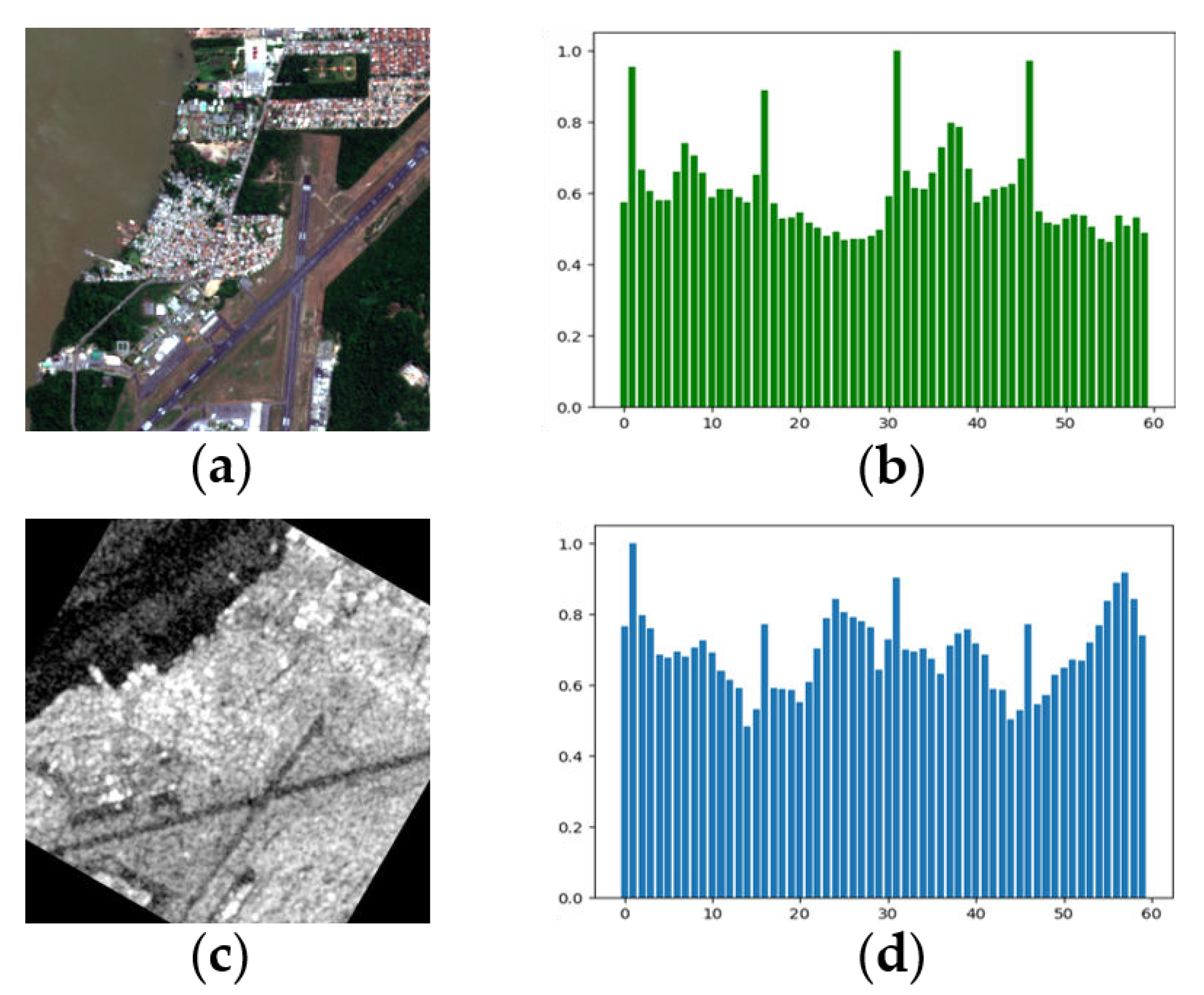
In Figure 1, for the existence of the rotation difference and the speckle noise between the optical and SAR images, it can hardly find the relationship from the histogram of two gradients directly. However, since the histogram of gradients should still contain information about the rotation of the images, we propose a novel network as RotNET based on the structure of a double-branch framework and the histogram as input, to find the rotation relationship between two images. With two branches sharing parameters with each other, the Siamese network can achieve good performance if added in the matching algorithms. However, in a certain optical-SAR image registration task, the Siamese network can be extremely limited by the speckle noise, leading to the occurrence of a series of other problems.
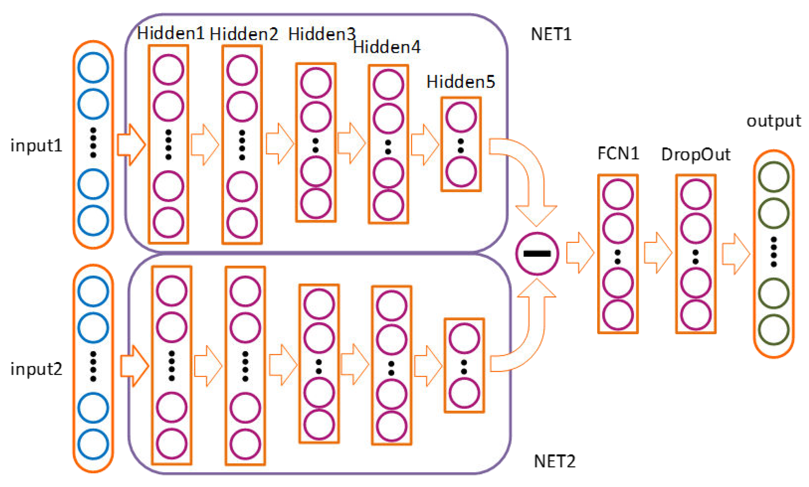
In Figure 2, the architecture of our network is consisted of the input layer, several hidden layers, fully-connected layers with dropout, and the output layer. The input of RotNET is the histogram of gradients, on account that the histogram contains the rotation property of the image. Compared with convolutional neural networks (CNN), this structure can effectively reduce some additional errors caused by image size. The NET1, same as the NET2, contains five hidden layers to extract the features of the histogram of gradient. Through NET1 and NET2, two sets of features are subtracted and then inputted into the fully-connected layers, which can further classify the deeper features of two inputs. Some details of each layer are presented in Table 1.
In Table 1, the RotNET has five hidden layers, and particularly, the output format is similar to image classification. The advantage comes that it is easier to quantify the training data and validation data with the design of classification. We divide 360 degrees into 128 classes, so the resolution of RotNET is 2.8 degrees.
2.2. The Creation of Training Data
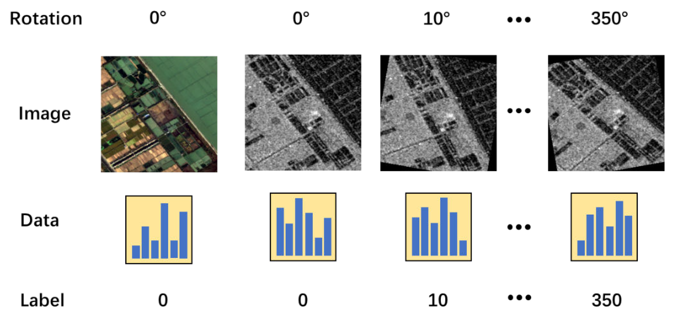
Up to now, there was not a neural network structure designed for predicting the rotation relationship between optical and SAR images like RotNET. Similarly, there was no available dataset for training the RotNET. However, for researching the data fusion of the SAR-Optical, M. Schmitt and the other researchers produced the SEN1-2 dataset [36]. It is comprised of 282,384 SAR-optical patch-pairs acquired by Sentinel-1 and Sentinel-2. In this paper, we use the SEN1-2 to create our own dataset. Because the image patch in SEN1-2 combined with the 30m-SRTM-DEM, the ASTER DEM for high latitude and the other methods to revise the image patch, we set the image patch in the SEN1-2 dataset to standard values. From Figure 3, the basic process is consisted of four steps:
- 1.
- Select data in the SEN1-2 dataset. Because the structure of RotNET is not complicated, taking part of the SEN1-2 dataset for training can have an excellent effect on predicting the rotation relationship between SAR and optical image. For our testing, it is taking only 2000 pairs of images to train RotNET that can achieve a satisfactory effect.
- 2.
- For each pair, SAR image rotates with its center from 0 degree to 360 degrees at an interval 5 degrees. Here we do not rotate the optical image, because we would like to predict the relative rotation relation.
- 3.
- After rotating the SAR image, we calculate the gradients of the images in the pair at both x-direction and y-direction and generate the magnitudes and orientations of gradients.
- 4.
- The histogram of each image is weighted the gradient magnitudes in the orientation by a trilinear interpolation method. In order to reduce the influence of illumination changes, the histogram is normalized by L2 norm.
In our dataset, the label of the image in each pair is the angle of rotation between the initial image and the image. The dataset only includes the positive data and labels. The negative samples can be generated by training strategies. The sample from different image pair can be regarded as the negative sample.
2.3. The Structure of Scale-Space and the Gaussian Pyramid
It has been shown by Lindeberg [37] that the Gaussian function is the only possible scale-space kernel for building the smooth scale space. is the function of the scale-space of the image:
is the input image. where * is the convolution operation between and . is Gaussian function which is:
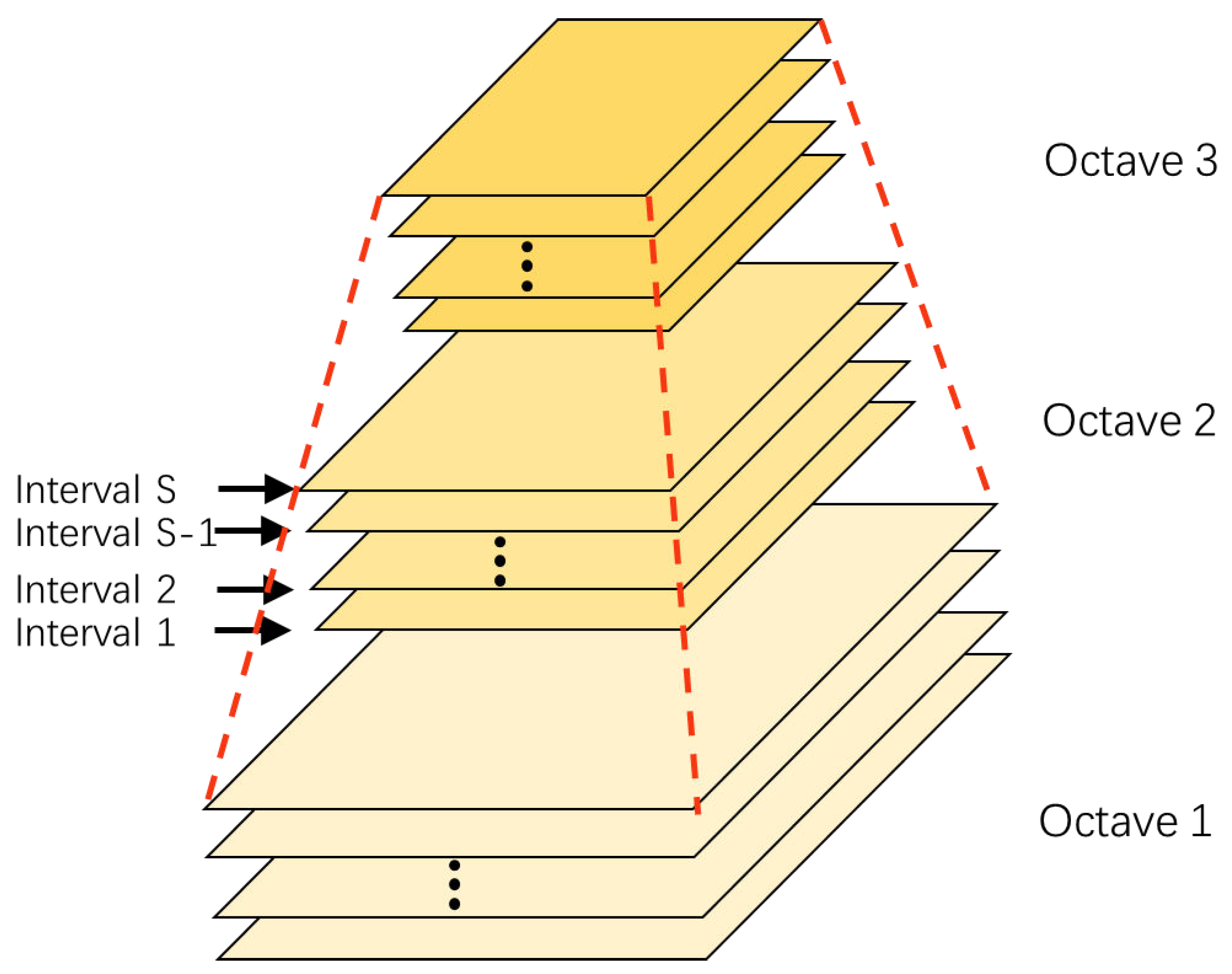
As shown in Figure 4, the Gaussian pyramid framework contains octave and interval scale spaces. The number of octaves (o) and the number of intervals (s) constitute the scale space. The Gaussian pyramid consists of two steps. In the first place, the initial image is convoluted with Gaussian functions whose coefficients are different to obtain an octave space. In the second place, the initial image in the next octave space is obtained by downsampling the last image of the previous layer.
For the octave pyramid space, the number of octaves is determined by the following equation:
O is the number of octaves, and (M, N) is the size of initial image. The last Gaussian blur coefficient in different octave spaces can be defined by
Similarly, for the interval space the Gaussian parameter of each image can be represented as:
where S is the number of intervals, and k is a constant. The Gaussian parameter of the image in the octave scale space is defined as follows:
The image that makes up the octave Gaussian pyramid can be represented as:
where and can be given by:
2.4. The Proposed of the GPOG Descriptor
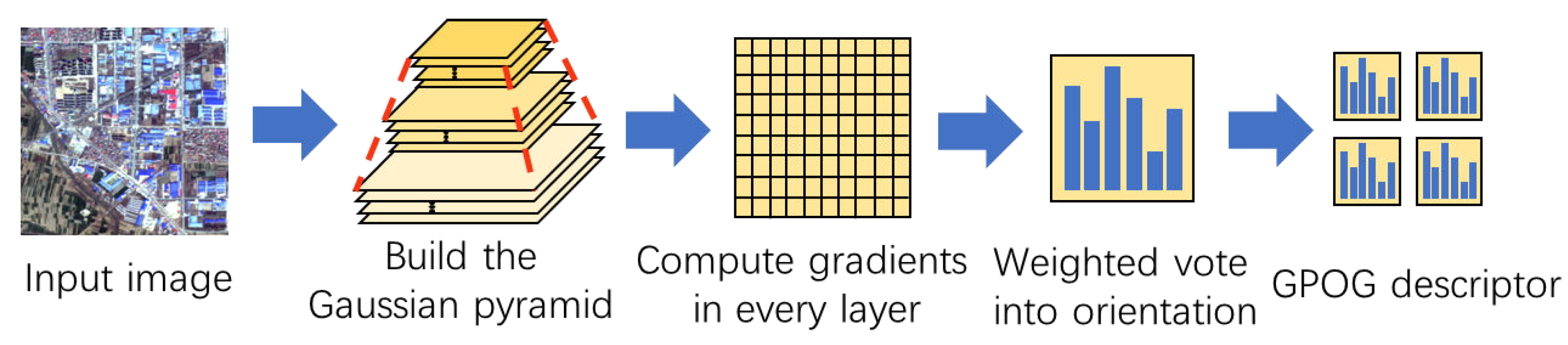
Inspired by the improvement of HOG, GPOG based on amplitude and orientation of gradient is proposed to describe local object appearances and shapes. HOG descriptor created the block-cell system to represent the structure of the image. For building the block-descriptor, we first need to divide the region into many cells, compute the histogram for each cell and collect them. Nevertheless, reducing the number of cells in one block can not generate more outstanding performance of the HOG descriptor than before. As computing efficiency increases, performance decreases. Through the block-cell structure, this HOG descriptor successfully magnifies the tiny difference between the two images. To achieve the one-cell block structure and accelerate the computational efficiency of the GPOG descriptor, Gaussian filters which have different variance are introduced to building the Gaussian pyramid. Following this, like HOG descriptor, we divide the image window into small spatial regions (one-cell block). For each block, we compute a local histogram of gradient directions and normalize the descriptor of the block descriptor. Then, we compose all of the block descriptor weighted by importance to obtain the GPOG descriptor. Figure 5 presents the main process of the proposed GPOG descriptor. The detailed steps of the process are as follows:
- 1.
- The first step is to apply Gaussian filters to the local region of each key-point in the optical and SAR image, and then make up the Gaussian pyramid which contains the information about the structure of the image. At the same time, the influence of the speckle noise of SAR image is able to be reduced by the Gaussian filter with downsampling. The octave number of the Gaussian pyramid is not too large, because the intensity of random noise is stronger than its structure information, as the downsampling and the Gaussian filter variance increases.
- 2.
- The second step is to calculate the x, y gradients in each layer, and then calculate the gradient amplitude and orientation. Because optical and SAR image gradients are in opposite directions, it should be noted that orientations need to be restricted to the range . In addition, this design is conducive to decrease the large intensity difference in optical and SAR image.
- 3.
- Dividing the whole layers in the Gaussian pyramid into some one-cell block, and calculating the local histogram of gradient directions in each block are showed in the third step. After that, the histograms normalized by the L2 norm in each block is utilized for obtaining a better performance to resist the illumination changes. To calculate the feature vector of the one-cell block, we use the method of trilinear interpolation to vote the gradient directions in each orientation. Moreover, the number of bins is not too large. The large bins number means less robust to the NRD and increases the computation extremely.
- 4.
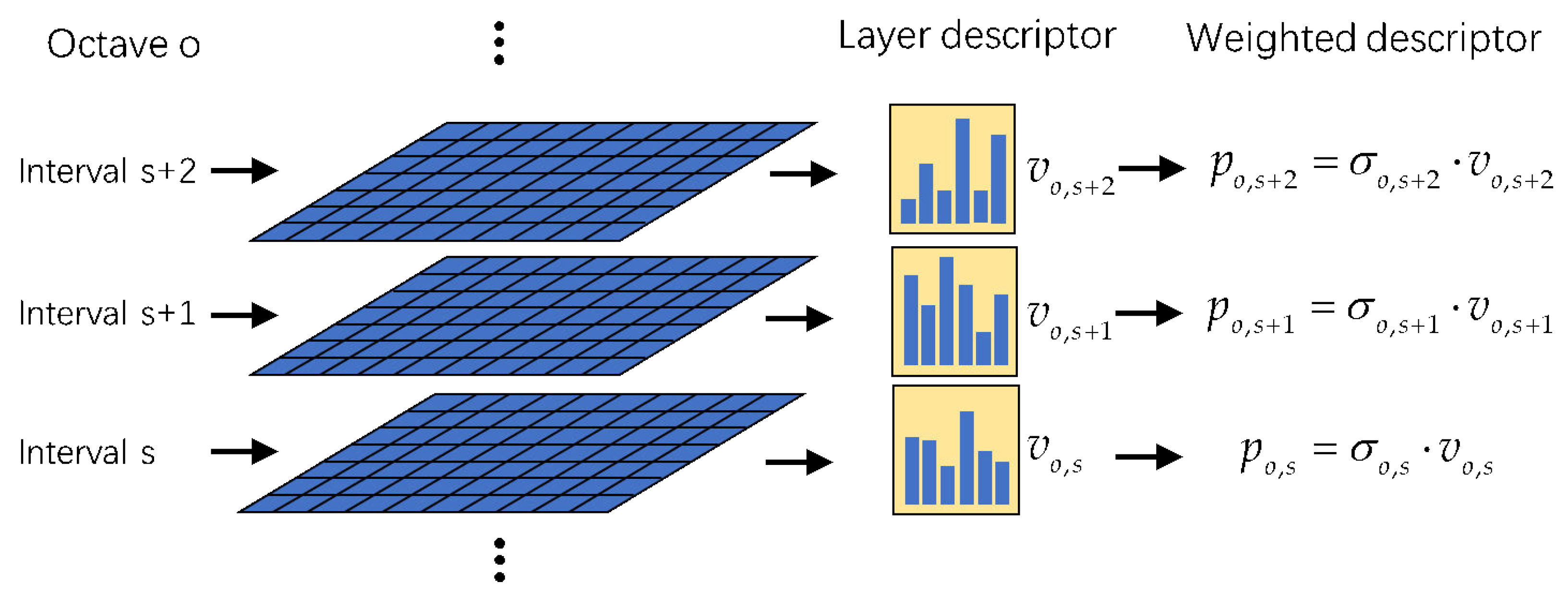
- The fourth step is to combine the block feature vector in each layer. In the Gaussian Pyramid, the larger number of the variance in Gaussian filter is, the higher the number of levels will be. It will be showed the fewer details and the more obvious edges. For emphasizing the importance of the obvious edges in the GPOG descriptor, the variance in the Gaussian filter is used as the weight to plus the block feature vector in the layer. Figure 6 presents the process of the weight in different layer.
- 5.
- The final step is to combine the layer feature vector in the Gaussian pyramid and obtain the proposed GPOG descriptor .
3. Experimental Results and Discussion
In this section, we design an experiment to evaluate the performance of the RotNET on different image pairs at SEN1-2 dataset. Furthermore the eight pairs of optical and SAR images are used to measure the RotNET in normal size image and analyze results. In the third experiment, we utilize different algorithm to calculate the similarity curve in six image pairs and analyze the convergence, including GPOG, HOPC and the other algorithms. The experiment is applied to evaluating the performance of algorithms in real-life tasks and analyzing the registration performance. All the experiment has been performed on a computer with an Intel Xeon Silver 4110 CPU and 64 GB memory.
3.1. Performance Experiment of Proposed RotNET in Dataset
To test the ability of RotNET in rotation prediction, we designed two experiments to evaluate the performance apart from the training experiment. In the first test, we select 100 images randomly from 6 sub-datasets of SEN1-2, and input them into the RotNET after certain rotation. In the second test, several other optical and SAR images from different satellites with different resolutions are randomly rotated and then also inputted into the RotNET to test the generalization ability of the model.
3.1.1. Evaluation Criteria of the Rotation Algorithm
Since RotNET is essentially a classification network, accuracy is used as the evaluation standard in this experiment. The accuracy is defined as
In the formula, D is dataset including and is the algorithm. ∏ is the indicator function and m is the sample size. is the accuracy number which ranges from 0 to 1 where 1 means this function is a perfect classifier.
3.1.2. Datasets of the Rotation Experiment
In the second experiment, we use four image pair from the SEN1-2 dataset. The resolution of these images is better than 5 m/pixel. The image size of six image pairs is 256 × 256 pixels. These images are named as pair 1 to 6. These images are not involved in the training of the network model, so the prediction accuracy can reflect the ability of the network.
3.1.3. The Result and Discussion of the Rotation Experiment
- Average loss for training data
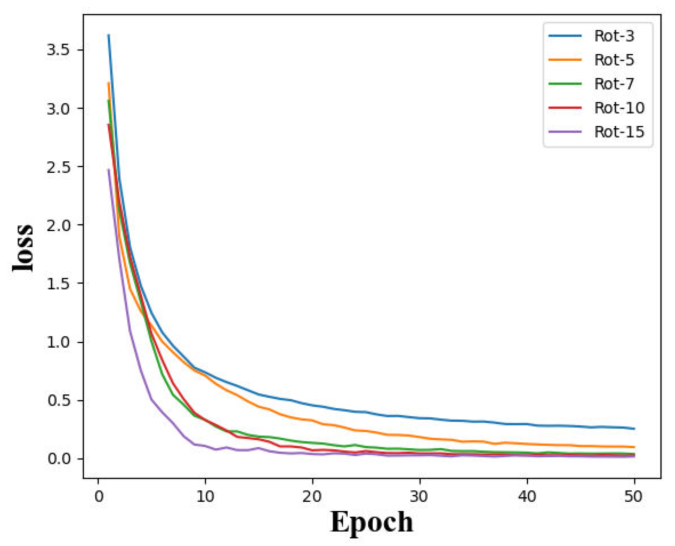
In the first experiment, we give the convergence of loss function under different precision conditions. We test 3°, 5°, 7°, 10°, 15° precision in the RotNET named Rot-3, Rot-5, Rot-7, Rot-10, Rot-15.
- Average loss for training data
In the first experiment, one thousand images from summer-18 and spring-50 were used in our training dataset. We test 3°, 5°, 7°, 10°, 15° precision in the RotNET named Rot-3, Rot-5, Rot-7, Rot-10, Rot-15 and give the convergence of loss function under different precision conditions.
Figure 10 shows the loss function of each epoch for the training data with different precision. Loss functions of all networks converge smoothly and fast. On the whole, the lower the resolution is, the faster the network converges and the better the prediction performance of the network.
- The performance in test data
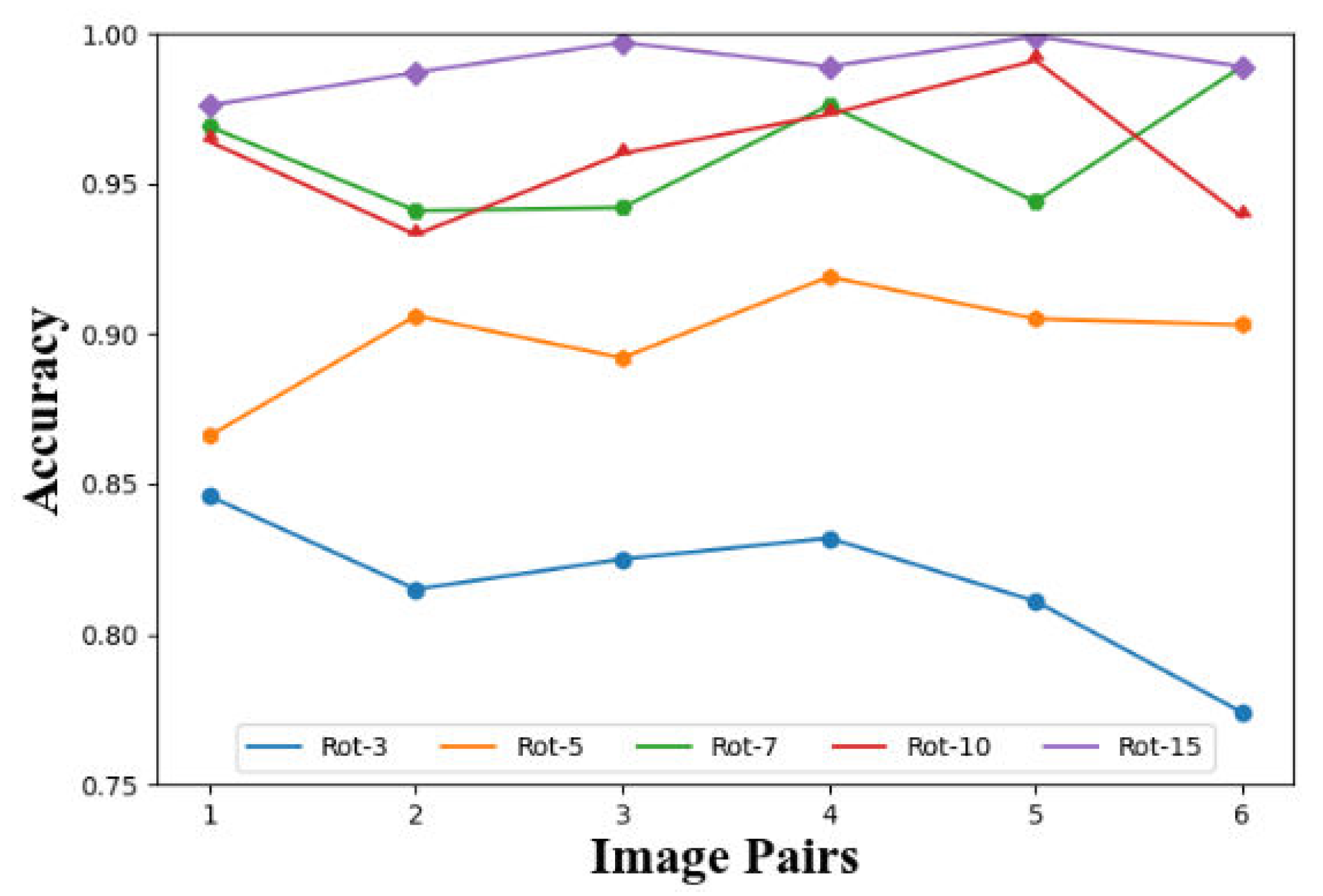
Six hundred images from spring-24, spring-98, summer-49, fall-29, fall-52, and winter-54 were used in our test dataset. As the Figure 11 shows, we calculate the histogram of the gradient distribution after rotating the image by a certain angle and input into the RotNET to test whether it can be correctly classified.
As the Figure 11 shows, the Rot-15 has the highest prediction accuracy in this test, because the lower resolution means the more obvious the histogram difference. The prediction accuracy in the Rot-15 is more than 98% in the six image pairs. The performance of the Rot-10 is worse than the Rot-15. However, in the image pair 1 and pair 5 the Rot-10 have similar abilities than Rot-15. The accuracy number of the Rot-10 is around 95% and it can still accurately predict image rotation. The Rot-7 performs similar to the Rot-10, with an accuracy of around 95%. Compared to the low resolution network, the prediction accuracy in the Rot-5 is significantly reduced to around 90%. Finally, the Rot-3’s prediction accuracy is around 80%.
Through the first and second experiments, with an input histogram resolution of 1°, the RotNET is able to accurately predict the rotation of the optical and SAR image. However, with the improvement of accuracy, the performance of the network has declined, but the overall accuracy is above 80%.
- The performance in real-world data
To test the performance of the RotNET in real-world image, we select three pairs of optical and SAR images with different resolutions and sizes.
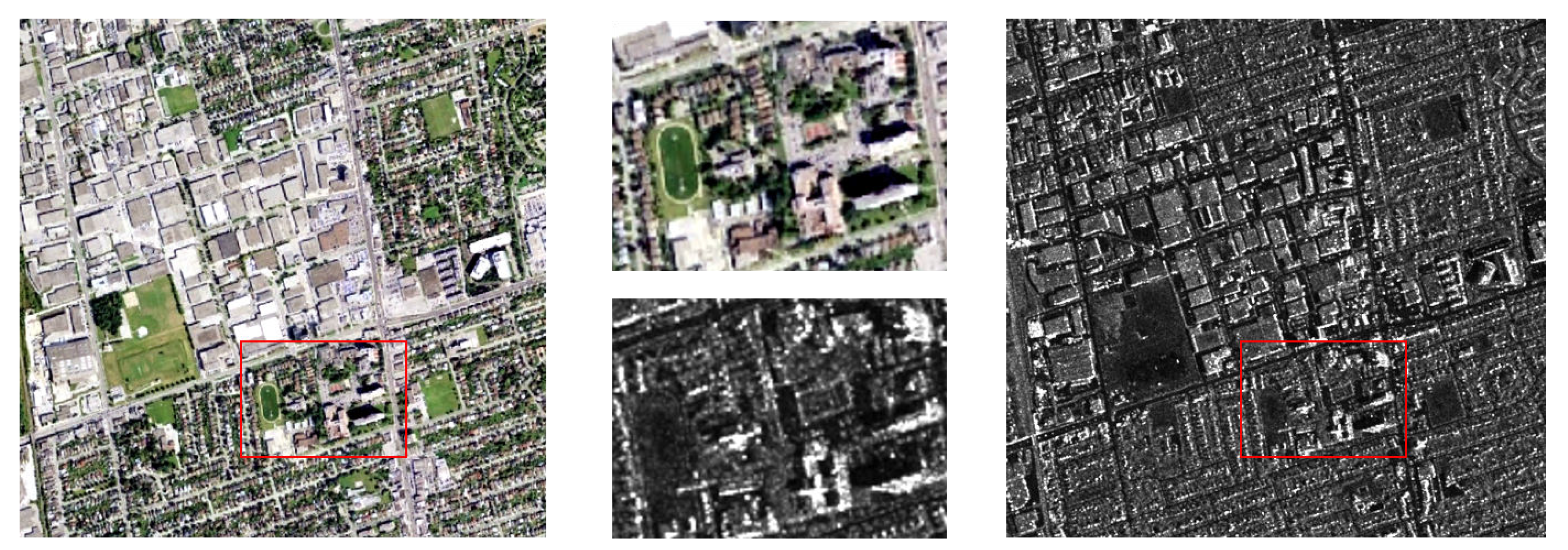
In pair 1, the size of the optical image and SAR image are 558 × 485 and 559 × 488. Because of the irradiance difference between the two images, the texture difference between the two images is huge. The fields can be seen clearly in optical images, but not in SAR images. As is shown in Table 2, the Rot-15, the Rot-10, the Rot-7 can still be accomplished correctly. The Rot-5 and Rot-3 get it right 50% of the time.
In pair 2, the size of the optical image and SAR image are 753 × 657 and 1052 × 779. Because of the different imaging modes, optical image and SAR image have different imaging sizes for the same ground object. As is shown in Table 3, it results in a SAR image being more than 200 pixels longer than the optical image. Under the circumstance, all of the test networks have good performance in this pair. Only the Rot-5 and Rot-3 have a wrong example.
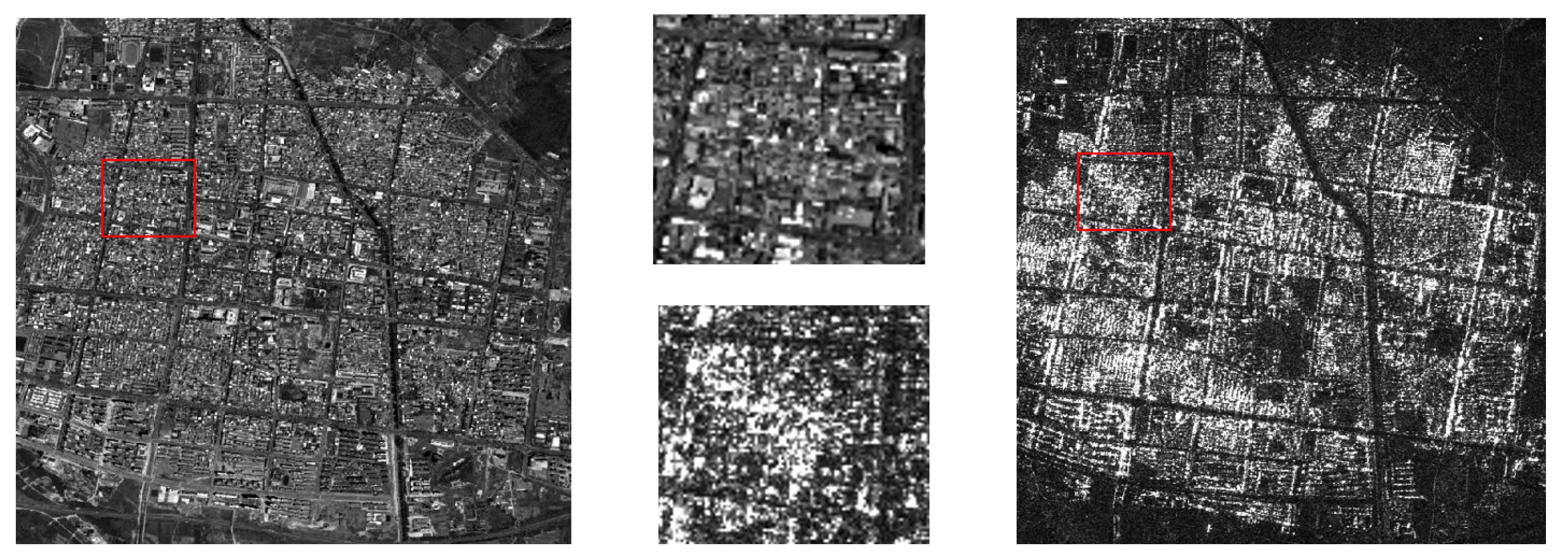
In pair 2, the size of the optical image and SAR image are 564 × 535 and 525 × 522. On account of the low resolution of the image, high-rise buildings in the urban area form interference in the SAR image, resulting in high noise of the SAR image. As a result, only the road can be used to distinguish the rotation relationship between the optical and SAR images. As is shown in Table 4, all of the test networks expect the Rot-3 having good performance in this pair. The Rot-3 get it right 50% of the time.
In summary, the RotNET has a strong ability to predict the rotation relationship between optical and SAR images in the dataset. In the same time, the RotNET have strong generalization capabilities. It can be seen from the third set of experiments that RotNET has good resistance to the irradiance difference between optical and SAR images, and the neural network is indeed able to find the rotation relationship stably through training. Through the above experiments, the RotNET has a better performance in this experiment because of two reasons, which are listed below:
- Although the irradiance of optical and SAR images is different, the gradient histogram contains the corresponding rotation relationship. The representation of histogram can abstract the image and prevent the influence of image size on the task.
- The double-branch neural network similar to Siamese network can fully extract the information generated by optical and SAR gradient histograms and predict the relative rotation relationship between them.
3.2. Performance Experiment of Proposed GPOG Descriptor
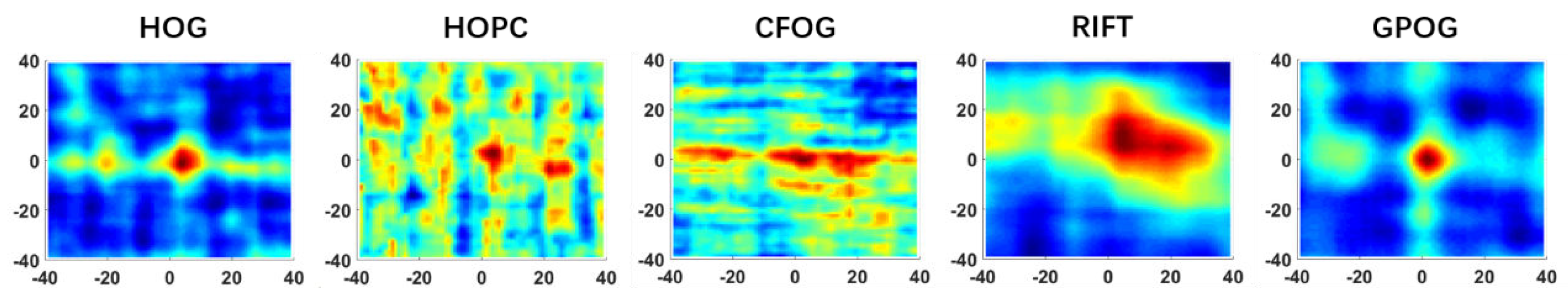
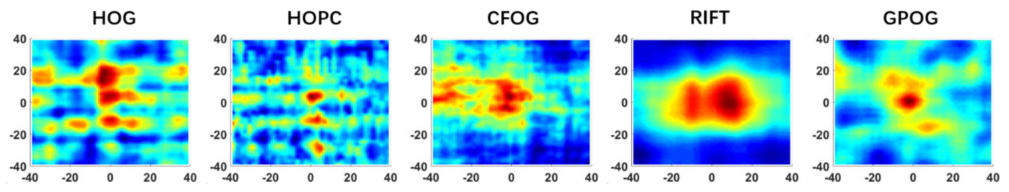
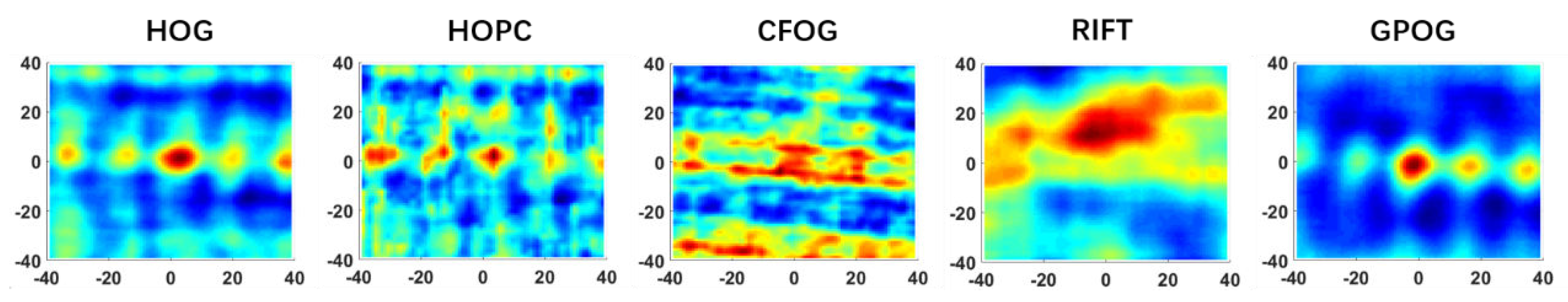
To test the accuracy of positioning of GPOG descriptor, we calculate similarity map of GPOG descriptor and compare with four other algorithms, namely RIFT, HOG, HOPC, channel features of orientated gradients (CFOG) [38]. PC map is used by the RIFT and HOPC to propose the descriptor. The block-cell system is uesd by the HOG, HOPC, and CFOG to exhibit good performance on multi-sensor image registration. The similarity map can qualitatively represent the structural expression ability of similarity metrics. By using the similarity map can we find the sensitivity of the structure in the descriptor.
3.2.1. Evaluation Criteria of the Similarity Map
As mentioned above, the GPOG descriptor is a feature descriptor, which is used in template registration. In this registration task the descriptor needs to break through significant non-linear radiometric differences when both images have similar structures. We use the normalized cross correlation (NCC) of the descriptor as the similarity metric for this task. The NCC is defined as
In the formula, and are the feature descriptor between optical and SAR images when and are the means of and . is the NCC number which ranges from −1 to 1 where 1 means the most relevant between two feature descriptors.
3.2.2. Experimental Data and the Test Process
- Experimental Data
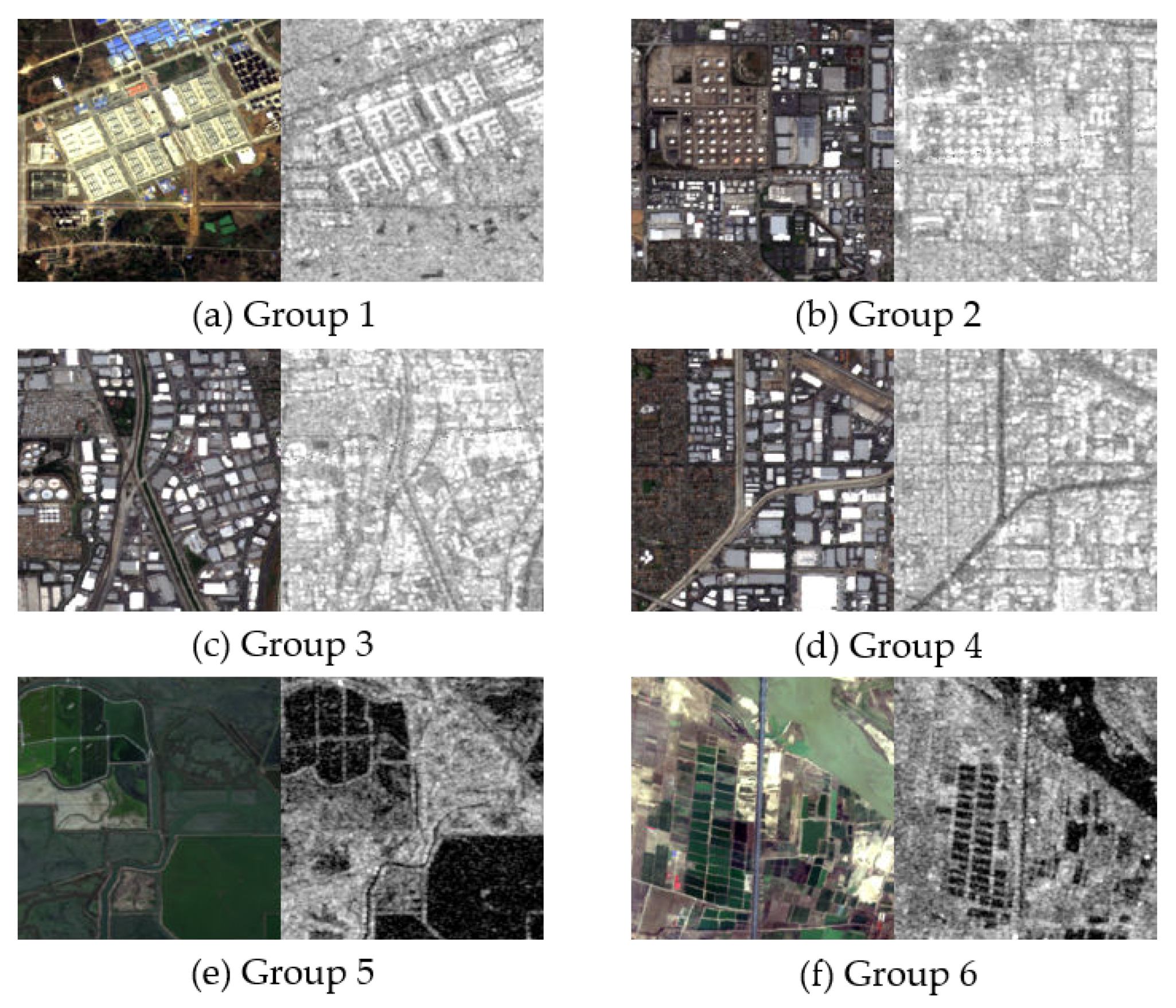
The similarity measurement experiment requires that the two images have the same position accuracy. Thus, we use the image pair from the SEN1-2 dataset. The resolution of these images is better than 5 m/pixel. We select six image pairs with 256 × 256 pixels. These images are named as Groups 1 to 6, as shown in Figure 12.
- The Test Process
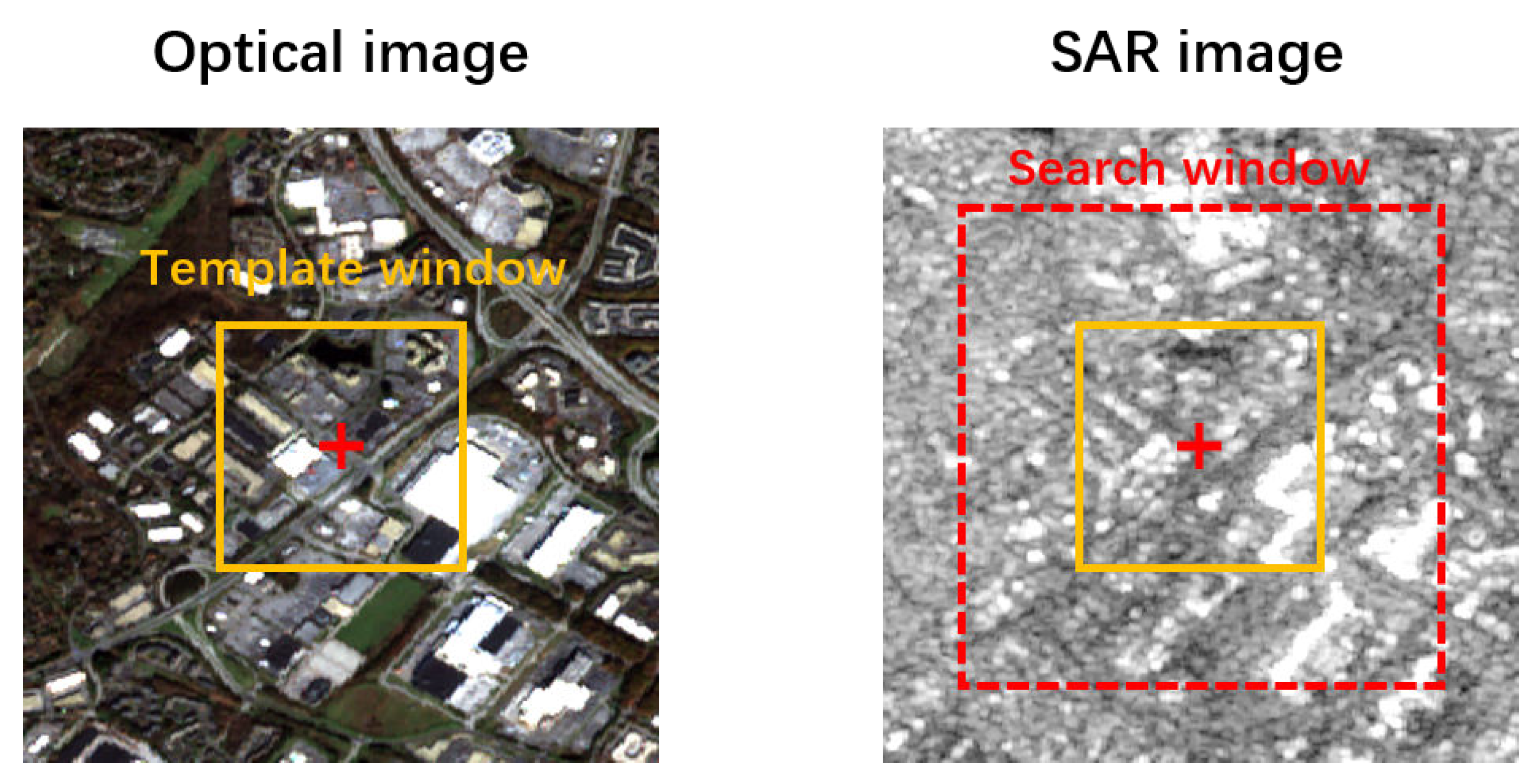
In this experiment, the optical image is the based image when the SAR image is the warp image. As is shown in Figure 13, the first step is that using the template window which has the same center as the based image to calculate the descriptor which be tested. The second step is that moving the template window in the search window from the begin to the end and calculate the descriptor at the same time. The third step is calculating the NCC between optical descriptor and SAR descriptor to structure the similarity map.
- Parameter Settings
In the process of test, the template window size is 100 × 100 pixels and the search window size is 80 × 80 pixels in each group. For the GPOG descriptor in this test, the Gaussian blur parameter is set to 2, the number of octaves O is set to 2, the number of intervals S is set to 3, the block size is 3 × 3 pixels. Based on the previous experience, the number of octaves is not too large owing to the increase in the noise as octaves have been added. Parameters of the other modal used in this experiment follow the parameter settings suggested by authors in their articles. The RIFT and HOPC descriptor are both based on PC. The Log-Gabor filter [39] is calculated in four scales, six orientations and 3 pixels smallest wavelength. Besides, in the HOPC and HOG descriptors the cell size is 3 × 3 pixels, the block size is 3 × 3 cells and the overlap number is 1.
3.2.3. Experimental Data and the Test Process
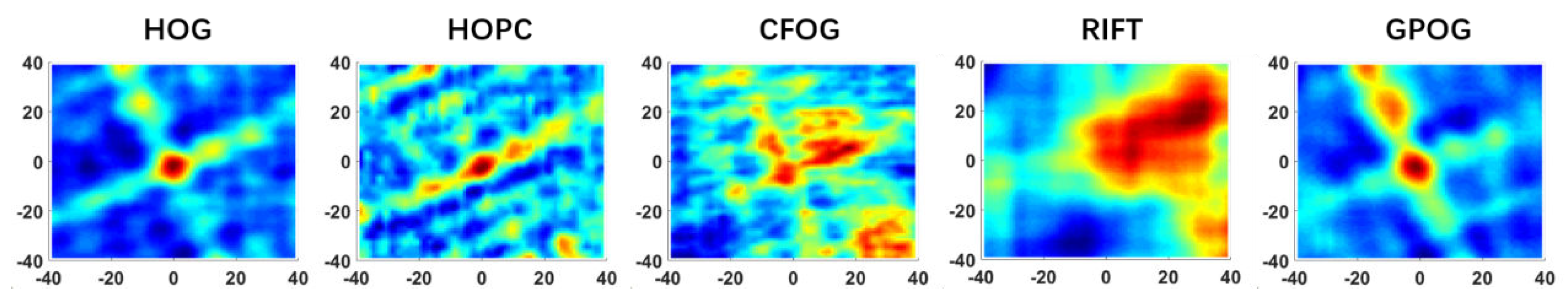
In order to effectively display, similarity maps are normalized. The darker the red is, the closer the number of NCC gets to 1. The darker the blue is, the closer it gets to 0. Therefore, the center region is 1 and the rest region is 0 is the ideal situation.
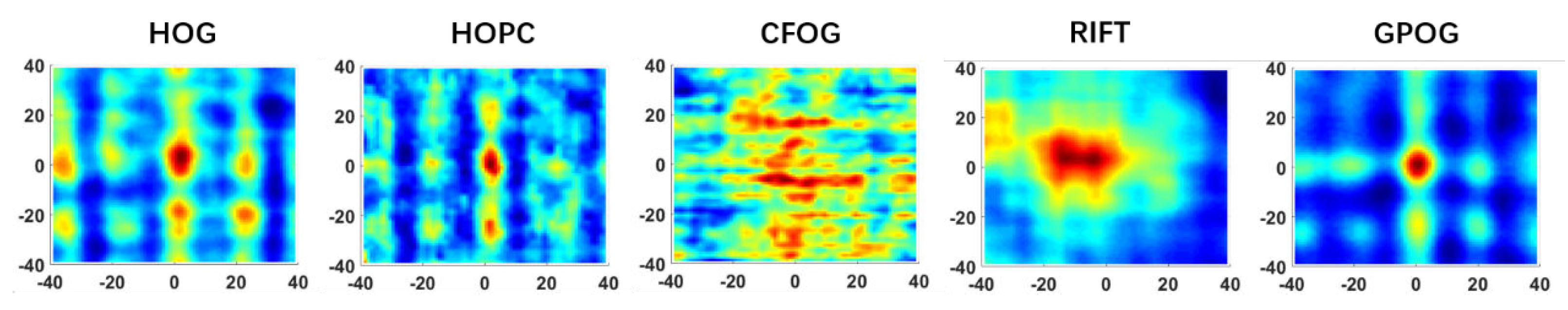
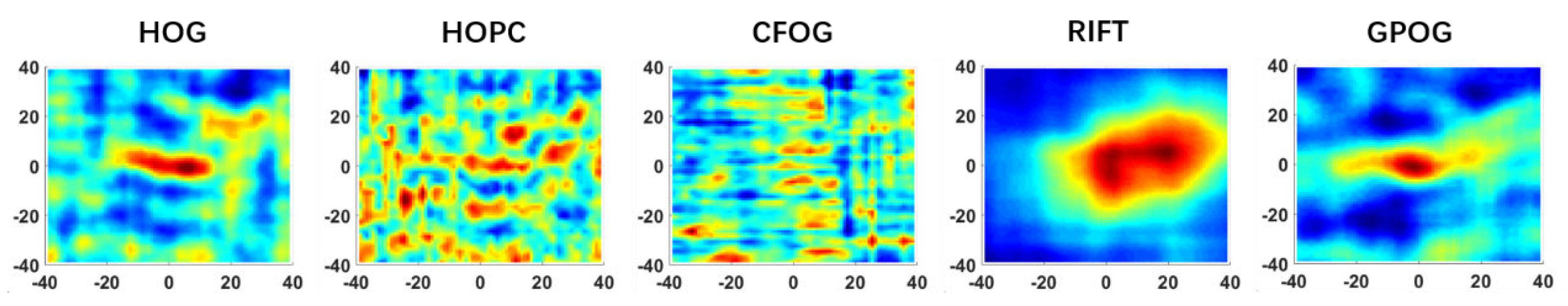
The results of the similarity map used six pairs of optical and SAR images are shown from Figure 14, Figure 15, Figure 16, Figure 17, Figure 18 and Figure 19. Because the center of the image in six groups is not all corner points and HOG, HOPC, CFOG and GPOG descriptors have good performance in this experiment, the accuracy of point matching can be further improved.
In Group 1, only HOG, HOPC and GPOG descriptors have a single peak on the center of the map. In Group 2, Because of the increased detail in the image all of descriptors can have a peak on the center, but the peak from RIFT is not sharp like the other descriptors. In Group 3, on account of the existence of the strong reflection point from SAR image, the information extracted from road features is the more important than other information. The HOPC and CFOG descriptors have not a prominent peak in the similarity map. In Group 4, On the contrary, the performance of the HOPC descriptor is superior to Group 3, because the strong reflection phenomenon in SAR is not strong and the house structure is clear in the SAR image. Because Group 5 is imaging on the farm land, structure is simple and easy to describe. Thus, all of descriptors have a single peak on the center of the map. In the final Group, the HOG, HOPC, and GPOG descriptor have a sharper peak than the others.
The comparison of the similarity map of the five descriptors indicates that the proposed GPOG descriptor has the most stable performance. It is more robust to the speckle noise and the less detail structure. The reasons are listed below.
- The Gaussian Pyramid separate the information in the pyramid structure by utilizing the scale space to distinguish between the obvious structure and the detail structure. The obvious structure includes road and river and so on, and the detail structure mainly includes the small house;
- The robustness to the noise can be availably improved by giving more weight to the obvious and information. In the meantime, the detail in the ground pyramid can provide the locating information, which gives the GPOG descriptor more resolving power;
- The difference between the optical and SAR images can be enlarged by the one-cell block system. On the one hand, smeller statistical units are more sensitive to the change. On the other hand, the smell structural is more sensitive to the speckle noise. The Gaussian filter can reduce the speckle noise effectively.
3.3. Performance Experiment of the Proposed Algorithm
To evaluate the performance of the RotNET and GPOG descriptor, we compare the GPOG descriptor with the HOG and RIFT descriptor in real world task. In this section, the performance of the registration algorithm can be evaluated by using subjective and objective criteria.
3.3.1. Evaluation Criteria of the Registration Algorithm
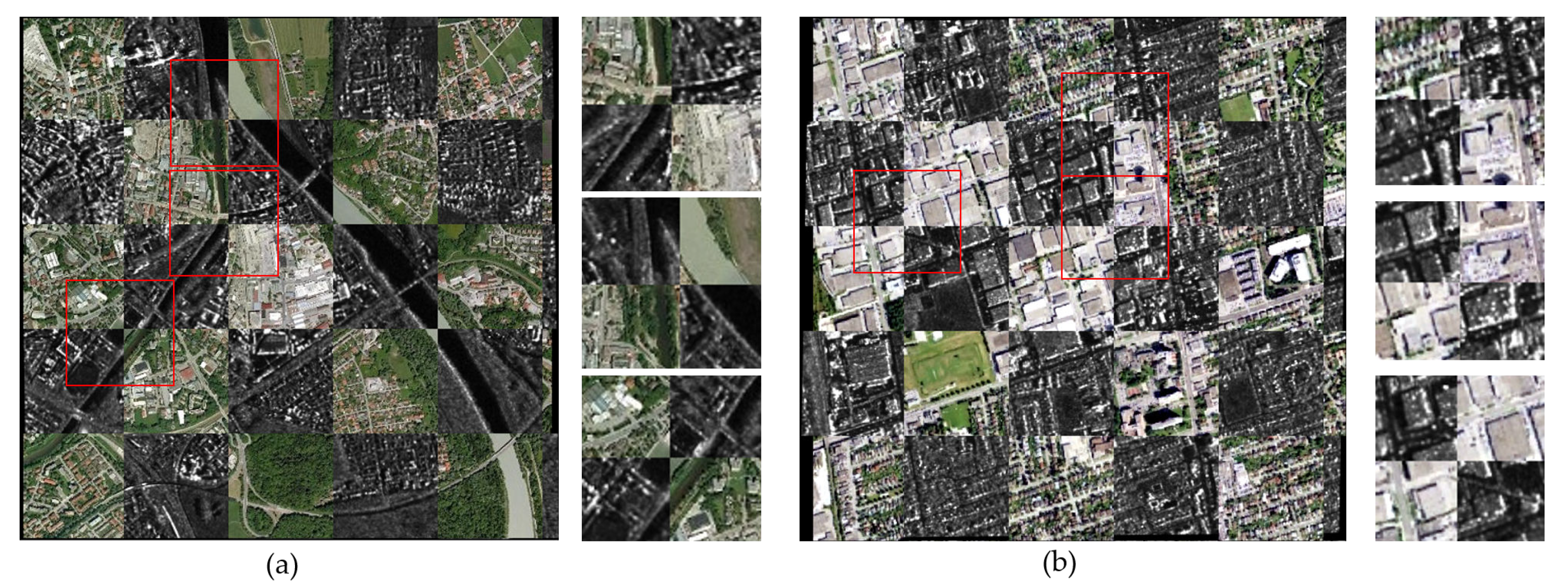
In this experiment, the performance of the registration algorithm is evaluated by three ways. The first method is using the checkboard mosaic image between the based image and warp image, and it is clearly to observe the detail of the image registration result.
In this experiment, we evaluate the performance of the registration algorithm in three ways. The first method is the checkboard mosaic image between the based image and the warp image which can observe the detail of the image registration result.
The second method is an objective and quantitative measure named Root mean square error (RMSE) [40] which can measure the coherence of the image registration, and is defined as following equation:
is the number of the matched point pairs in the image pair. T is the transformation matrix computed by the whole matched point pairs in the image pair.
RMSE reflects the matching accuracy of optical and SAR images. The smaller the RMSE is, the more accurate the matching results will be. However, the number of match points should be considered when using the RMSE criteria.
The third method is to use number of correct matches (NCM). The NCM is the number of match points after removing wrong points. The NCM must be more than four because we use the affine transformation to fit optical and SAR images.
3.3.2. Datasets of the Registration Algorithm
Six pairs of optical and SAR images are used to test the GPOG descriptor in this section. The Table 5 gives the details of each cases.
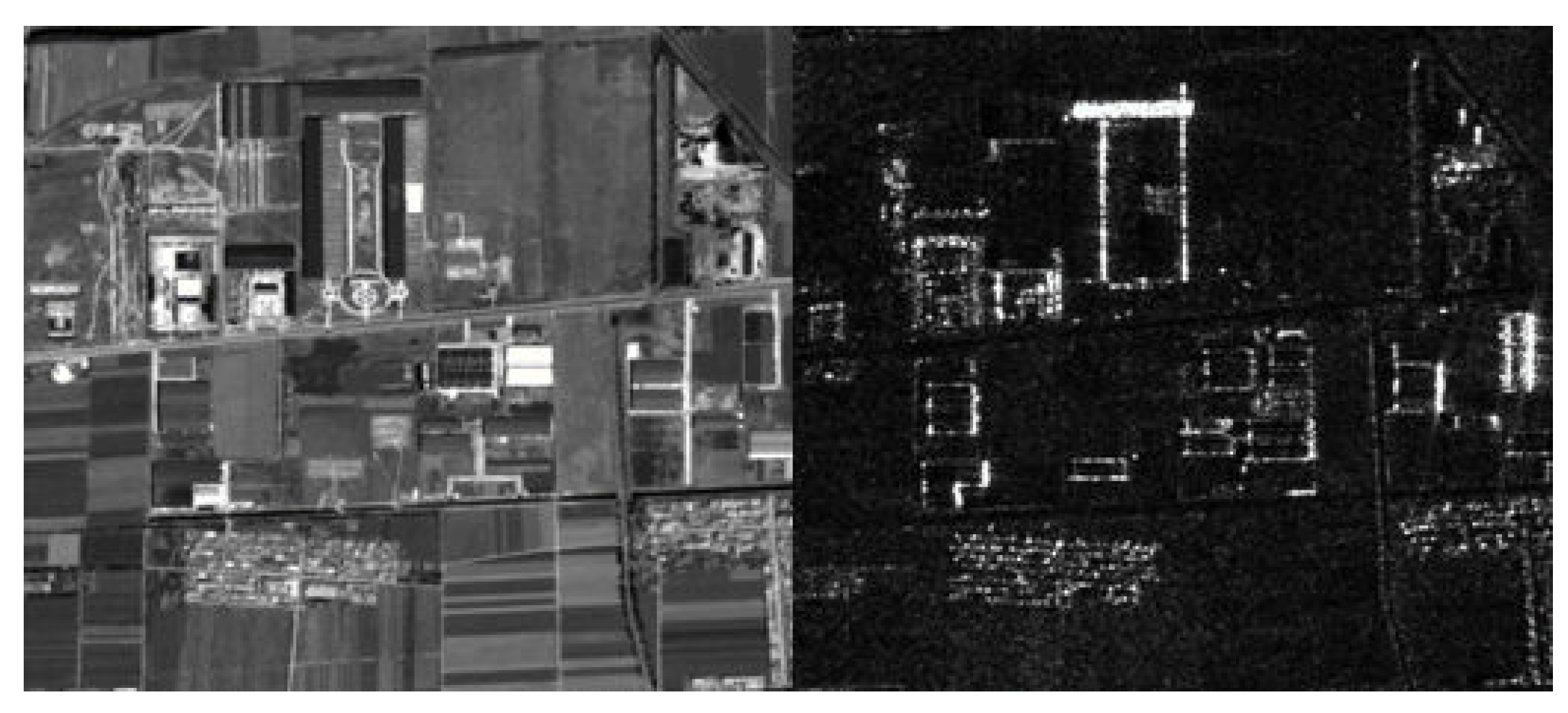
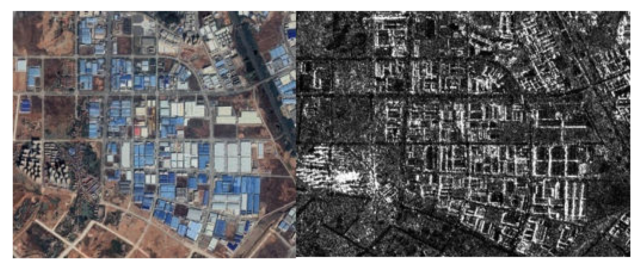
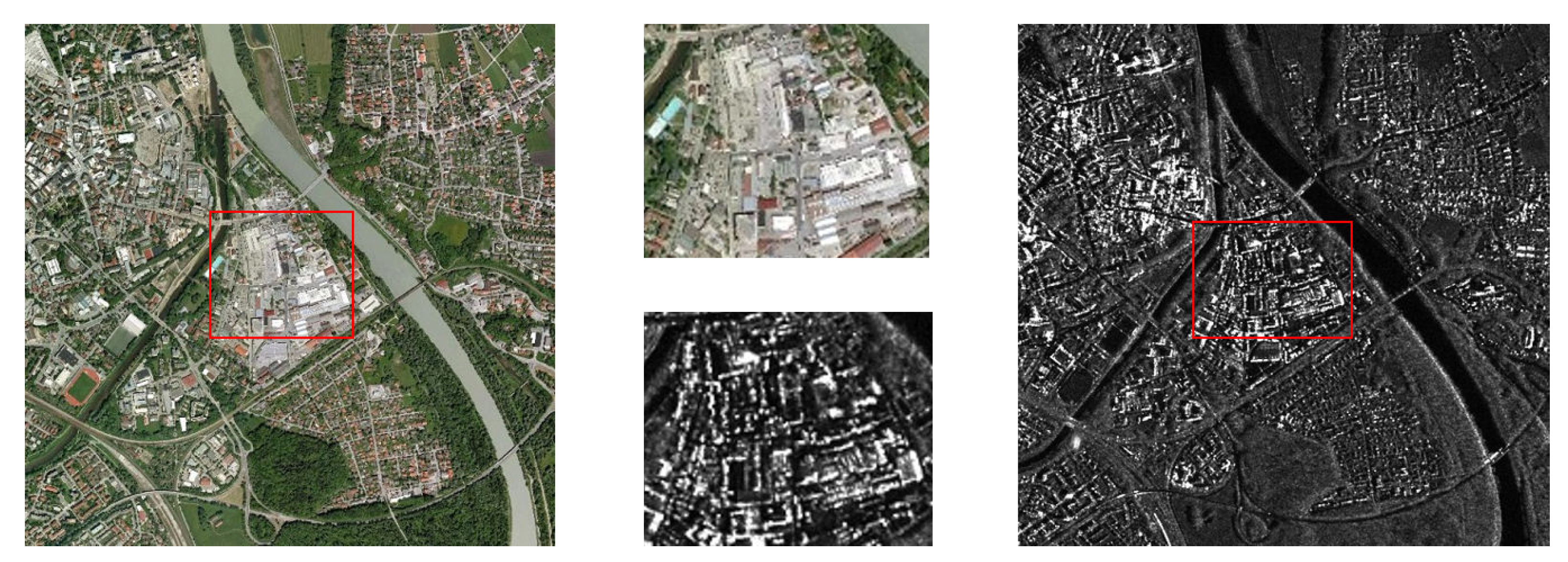
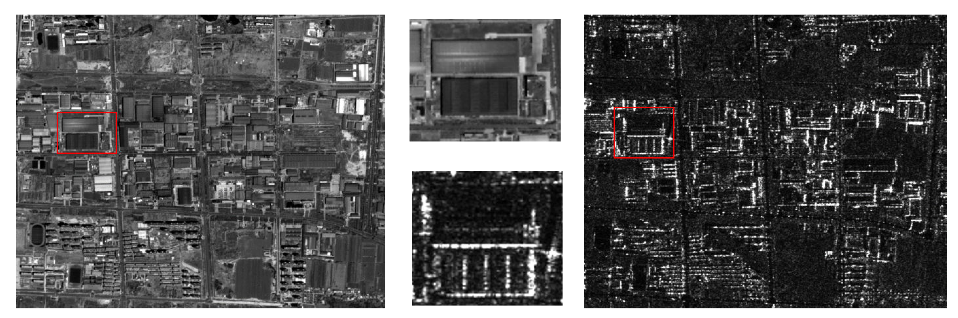
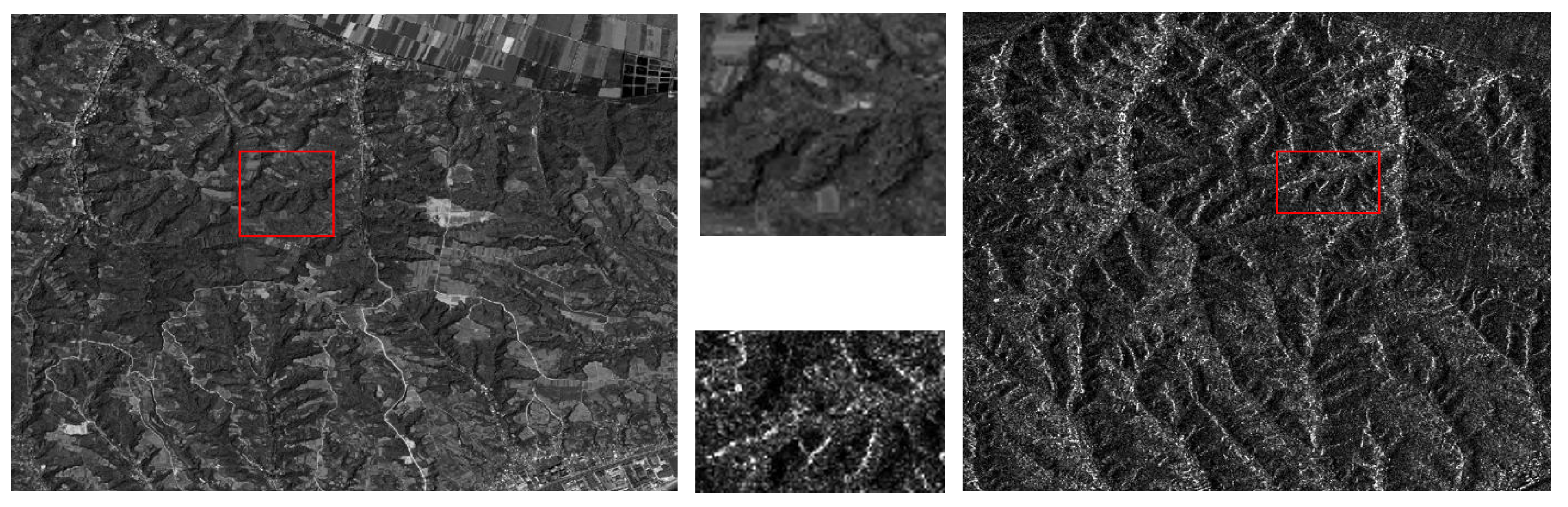
The optical images in the six pairs are from Google Earth, and the SAR images are obtained from the TerraSAR-X satellite and the airborne image. As shown in Figure 20, Figure 21, Figure 22, Figure 23, Figure 24 and Figure 25, to analyze the performance of the proposed matching framework, the imaging date, the resolution, the size, details and the noise level between the test data are different.
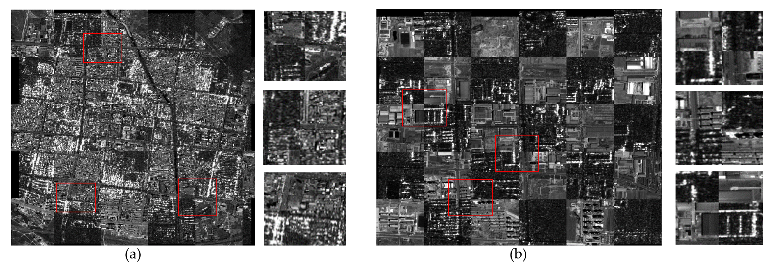
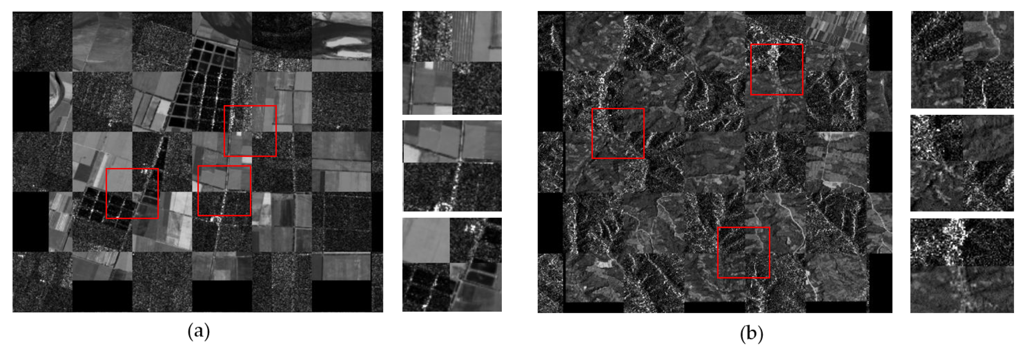
Pair B and pair A both include images of a long river, bridges, roads and houses which have sharp edges. They are the best quality images in six pairs, because the noise in SAR images is at a low level. Obtained from Hunan, the existence of roads and high buildings in pair C cause a large amount of interference in SAR images and make it difficult to obtain clear images. In pair D, the images with suburban areas have a high resolution. However, high resolution is not necessarily a good thing for template matching, the higher the resolution is, the less information corresponding to the same template will be. Pair E includes images of lots of cropland which have the similar texture and details. Images of mountainous areas that is hard to match with human eyes are included in pair F. In conclusion, six pairs in this experiment have different sensor, imaging time, resolution, the level of noise, and geographical structure.
3.3.3. Comparison of Experimental Results
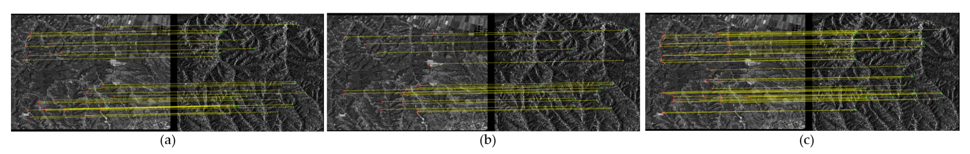
To analyze the performance of the GPOG descriptor in optical and SAR registration, we compare it with RIFT and HOG algorithm. The RIFT descriptor represents the application of phase congruence and MIM, which is robust to the NRD. The HOG descriptor represents cell-block system which can describe the image structure correctly.
For the sake of ensuring the fairness and rigor of the experiment, the variables are controlled in this experiment. We use FAST corner detector to extract feature points (approximately 1000) in all of the test. Then, we make use of the fast sample consensus (FSC) algorithm [41] to remove false matches. In the whole experiment, only the descriptor is different and the other variables are exactly the same. The registration results of six pairs are shown in Figure 26, Figure 27, Figure 28, Figure 29, Figure 30 and Figure 31.
In order to observe the registration effect, we put the checkboard mosaic images and sub-images which can reflect the accuracy of registration in Figure 32, Figure 33 and Figure 34.
For purpose of obtaining the quantitative comparison of strengths and weaknesses about RIFT, HOG, GPOG algorithms, RMSE, and NCM are used as objective evaluation indexes to evaluate the three algorithms. Table 6 lists RMSE and NCM results of six pairs in the experiment.
This experiment includes common geographical environments (houses, rivers, roads, and mountains) of remote sensing images. In these scenes, optical and SAR images have different irradiance characteristics and noise distributions. The most important problems are the signal-to-noise (SNR) within the scope of the template and the abundant details. According to its intensity, the noise can be classified as low noise and high noise. According to the abundant information in the template, it can be divided into strong texture and weak texture. Then, we evaluate the test results of six image pairs.
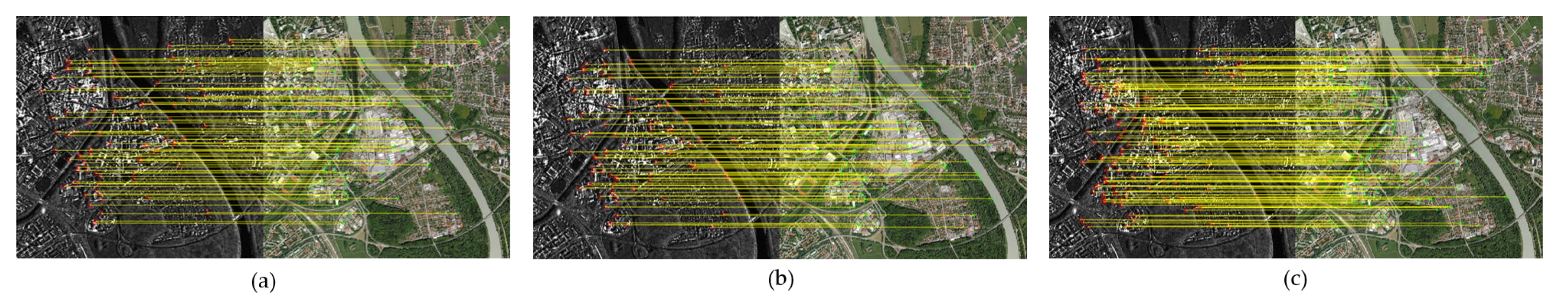
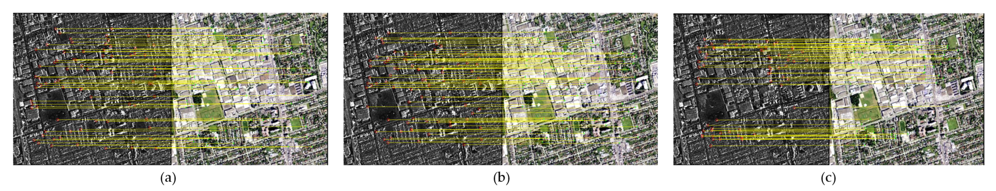
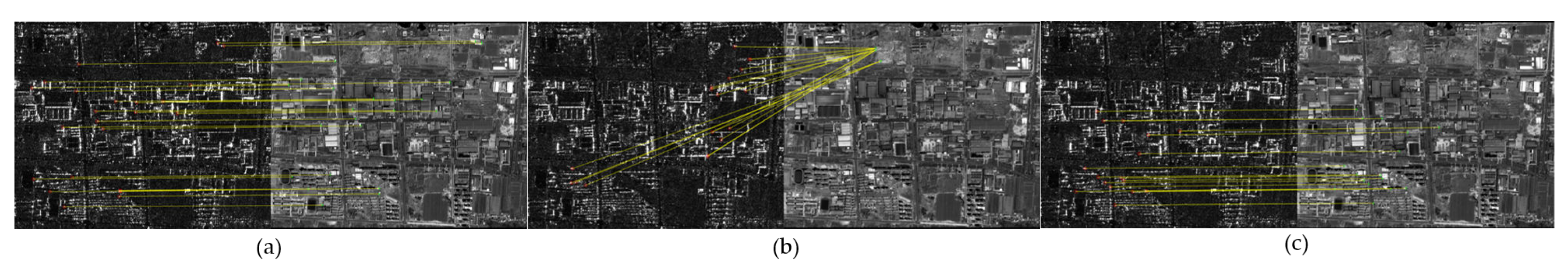
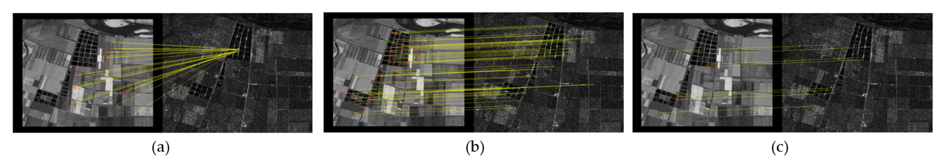
The images with urban area in pair A and pair B are represented the features of low noise and high texture. In these two groups of images, the three algorithms have achieved good results, and the GPOG descriptor can match more feature points than the other two algorithms. Similarly, the images with urban areas in third pair have lower resolution, which bring more speckle noise and more texture information. The images are categorized to high noise and high texture images. The stable feature points extracted by GPOG descriptor are 3–4 times higher than the other two algorithms, which is inseparable from the suppression of noise by its pyramid structure. In contrast to pair C, the images in the fourth group of experiments have characteristics of low noise, low texture, high resolution, and less information under the same template size. Because of less information, none of the three operators perform well as before. However, in comparison with HOG descriptor, the GPOG descriptor has a stronger ability to represent low texture information due to the amplification of the main information by the Gaussian pyramid, which make GPOG descriptor have similarity performance of RIFT descriptor based on Log-Gabor wavelet. The images with farmland area in the fifth pair are also presented the characteristic of low noise and low texture. However, in the fifth pair the performance of the HOG descriptor is similar to the GPOG descriptor, which indicates that HOG descriptor is more sensitive to the information within the template compared with the resolution and noise. Images in pair F is mountain images which classified as the type of high noise and high texture and it is difficult for human eyes to find the corresponding points in the two images. GPOG descriptor can also extract the most associated feature points. It further indicates that the Gaussian pyramid structure has achieved the desired result in noise suppression of multi-sensor images and extraction of important texture structures.
In summary, the RIFT descriptor uses Log-Gabor wavelet to describe the image texture, which is robust to both low texture and high noise. However, when the maximum index map is introduced to improve the robustness, it is insensitive to pixel level changes, resulting in a low positioning accuracy. The performance of this algorithm is dependent on the accuracy of feature point extraction algorithm. As a classical descriptor based on gradient information, HOG can magnify the difference between optical and SAR images because the cell-block system is capable of improving its positioning ability. However, as a pixel-level template matching algorithm, its performance depends on the abundant texture within the matching template and the SNR. Compared with previous two algorithms, GPOG descriptor has a better performance in this experiment because of two reasons, which are listed below:
- The GPOG descriptor uses the Gaussian pyramid structure to separate the main information in the template window. Only in this way, can the descriptor amplify the weak texture information to distinguish the images;
- By using the Gaussian filter, the speckle noise in the SAR image is suppressed. The structural information will be highlighted with the improvement of SNR.
3.3.4. Rotation and Scale Experiments of the Proposed GPOG Algorithm
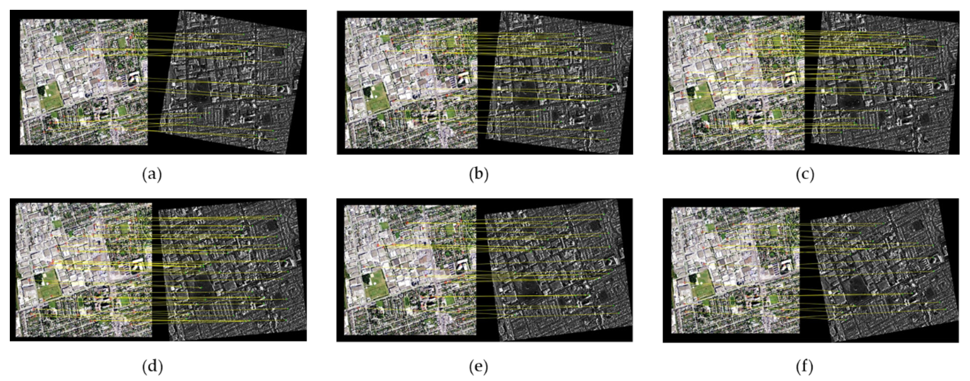
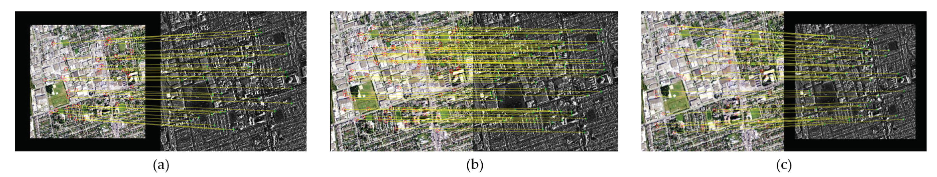
The previous experimental results show that GPOG descriptor is robust to the SAR speckle noise and NRD. The large-angle rotation between optical and SAR image can be corrected using the RotNET. Consider the RotNET resolution, the GPOG descriptor only needs to be resistant to small image rotations. In the first experiment, the influence of rotation on GPOG descriptor is evaluated based on NCM. In the second experiment, the influence of scale on GPOG descriptor is evaluated based on NCM.
4. Conclusions
In this paper, inspired by the structure of the Siamese network, we propose a novel neural network framework (named RotNET) to predict the rotation relationship between SAR and optical image. For training the RotNET, we constructed a dataset based on gradient histogram based on the SEN1-2 dataset. Then we build the GPOG descriptor by used the Gaussian pyramid that is able to build the scale space and extract the important feature. By making use of the one-cell block system in the Gaussian pyramid we propose the GPOG descriptor.
To validate the superiority of the proposed work, we carry out specific and quantitative experiments. First, we build our own dataset based on SEN1-2 dataset to train RotNET and respectively teste the RotNET with dataset images and real-world images. The experiment shows that the RotNET can find the rotation relationship between optical and SAR images, both in the dataset and in the real-world images. Second, we design two experiments to test the performance of GPOG descriptor. In the first test, we compare the GPOG descriptor with the other descriptors by similarity maps, and the results show that the applicability and convergence performance of GPOG are better. In the second test, we compare the GPOG descriptor with the other descriptors by using RMSE and NCM criteria, and the results show that GPOG descriptor is robust to SAR speckle noise and NRD.
The RotNET neural network framework can predict the rotation relationship ignoring the size of the two images and is applied to change detection, image analysis and image preprocessing. The GPOG descriptor can play a role in the image registration, fusion of multi-sensor images and image coding. In the future, we will test our RotNET and the GPOG descriptor on more multi-sensor images with irradiance difference, such as optical and light detection and ranging (LiDAR).
Author Contributions
Z.L. was primarily responsible for conceiving the method and writing the source code and the paper. H.Z. designed the experiments and revised the paper. Y.H. generated datasets and performed the experiments. All authors have read and agreed to the published version of the manuscript.
Funding
This research received no external funding.
Conflicts of Interest
The authors declare no conflict of interest.
References
- Kulkarni, S.; Rege, P. Pixel Level Fusion Techniques for SAR and Optical Images: A Review. Inf. Fusion 2020, 59, 13–29. [Google Scholar] [CrossRef]
- Ma, J.; Jiang, X.; Fan, A.; Jiang, J.; Yan, J. Image Matching from Handcrafted to Deep Features: A Survey. Int. J. Comput. Vis. 2021, 129, 23–79. [Google Scholar] [CrossRef]
- Tapete, D.; Cigna, F. Detection of Archaeological Looting from Space: Methods, Achievements and Challenges. Remote Sens. 2019, 11, 2389. [Google Scholar] [CrossRef] [Green Version]
- Song, S.; Jin, K.; Zuo, B.; Yang, J. A novel change detection method combined with registration for SAR images. Remote Sens. Lett. 2019, 10, 669–678. [Google Scholar] [CrossRef]
- Li, K.; Zhang, X. Review of Research on Registration of SAR and Optical Remote Sensing Image Based on Feature. In Proceedings of the 2018 IEEE 3rd International Conference on Signal and Image Processing (ICSIP), Shenzhen, China, 13–15 July 2018; pp. 111–115. [Google Scholar]
- Fan, J.; Wu, Y.; Li, M.; Liang, W.; Cao, Y. SAR and Optical Image Registration Using Nonlinear Diffusion and Phase Congruency Structural Descriptor. IEEE Trans. Geosci. Remote Sens. 2018, 56, 5368–5379. [Google Scholar] [CrossRef]
- Dare, P.; Dowman, I. An improved model for automatic feature-based registration of SAR and SPOT images. ISPRS J. Photogramm. Remote Sens. 2001, 56, 13–28. [Google Scholar] [CrossRef]
- Feng, R.; Du, Q.; Li, X.; Shen, H. Robust registration for remote sensing images by combining and localizing feature- and area-based methods. ISPRS J. Photogramm. Remote Sens. 2019, 151, 15–26. [Google Scholar] [CrossRef]
- Zitova, B.; Flusser, J. Image registration methods: A survey. Image Vis. Comput. 2003, 21, 977–1000. [Google Scholar] [CrossRef] [Green Version]
- Suri, S.; Reinartz, P. Mutual-Information-Based Registration of TerraSAR-X and Ikonos Imagery in Urban Areas. IEEE Trans. Geosci. Remote Sens. 2010, 48, 939–949. [Google Scholar] [CrossRef]
- Li, Z.; Mahapatra, D.; Tielbeek, J.A.W.; Stoker, J.; van Vliet, L.J.; Vos, F.M. Image Registration Based on Autocorrelation of Local Structure. IEEE Trans. Med. Imaging 2016, 35, 63–75. [Google Scholar] [CrossRef]
- He, C.; Fang, P.; Xiong, D.; Wang, W.; Liao, M. A Point Pattern Chamfer Registration of Optical and SAR Images Based on Mesh Grids. Remote Sens. 2018, 10, 1837. [Google Scholar] [CrossRef] [Green Version]
- Lowe, G.D. Distinctive Image Features from Scale-Invariant Keypoints. Int. J. Comput. Vis. 2004, 2, 91–110. [Google Scholar] [CrossRef]
- Rublee, E.; Rabaud, V.; Konolige, K.; Bradski, G. ORB: An Efficient Alternative to SIFT or SURF. 2011. Available online: https://0-ieeexplore-ieee-org.brum.beds.ac.uk/document/6126544 (accessed on 6 November 2011).
- Ma, W.; Wen, Z.; Wu, Y.; Jiao, L.; Gong, M.; Zheng, Y.; Liu, L. Remote Sensing Image Registration with Modified SIFT and Enhanced Feature Matching. IEEE Geosci. Remote Sens. Lett. 2017, 14, 3–7. [Google Scholar] [CrossRef]
- Bay, H.; Ess, A.; Tuytelaars, T.; Van Gool, L. Speeded-Up Robust Features (SURF). Comput. Vis. Image Underst. 2008, 110, 346–359. [Google Scholar] [CrossRef]
- Ke, Y.; Sukthankar, R. PCA-SIFT: A more distinctive representation for local image descriptors. In Proceedings of the 2004 IEEE Computer Society Conference on Computer Vision and Pattern Recognition, Washington, DC, USA, 27 June–2 July 2004; Volume 2, p. II. [Google Scholar]
- Morel, J.M.; Yu, G. ASIFT: A new framework for fully affine invariant image comparison. SIAM J. Imaging Sci. 2009, 2, 438–469. [Google Scholar] [CrossRef]
- Xu, C.; Sui, H.; Li, H.; Liu, J. An automatic optical and SAR image registration method with iterative level set segmentation and SIFT. Int. J. Remote Sens. 2015, 36, 3997–4017. [Google Scholar] [CrossRef]
- Sedaghat, A.; Ebadi, H. Remote Sensing Image Matching Based on Adaptive Binning SIFT Descriptor. IEEE Trans. Geosci. Remote Sens. 2015, 53, 5283–5293. [Google Scholar] [CrossRef]
- Dellinger, F.; Delon, J.; Gousseau, Y.; Michel, J.; Tupin, F. SAR-SIFT: A SIFT-Like Algorithm for SAR Images. IEEE Trans. Geosci. Remote Sens. 2015, 53, 453–466. [Google Scholar] [CrossRef] [Green Version]
- Xiang, Y.; Wang, F.; You, H. OS-SIFT: A Robust SIFT-Like Algorithm for High-Resolution Optical-to-SAR Image Registration in Suburban Areas. IEEE Trans. Geosci. Remote Sens. 2018, 56, 3078–3090. [Google Scholar] [CrossRef]
- Kovesi, P. Phase congruency: A low-level image invariant. Psychol. Res. 2000, 64, 136–148. [Google Scholar] [CrossRef]
- Morrone, M.C.; Owens, R.A. Feature detection from local energy. Pattern Recognit. Lett. 1987, 6, 303–313. [Google Scholar] [CrossRef]
- Ye, Y.; Shan, J.; Bruzzone, L.; Shen, L. Robust Registration of Multimodal Remote Sensing Images Based on Structural Similarity. IEEE Trans. Geosci. Remote Sens. 2017, 55, 2941–2958. [Google Scholar] [CrossRef]
- Dalal, N.; Triggs, B. Histograms of oriented gradients for human detection. In Proceedings of the 2005 IEEE Computer Society Conference on Computer Vision and Pattern Recognition (CVPR’05), San Diego, CA, USA, 25 July 2005; Volume 1, pp. 886–893. [Google Scholar]
- Ye, Y.; Shan, J.; Hao, S.; Bruzzone, L.; Qin, Y. A local phase based invariant feature for remote sensing image matching. ISPRS J. Photogramm. Remote Sens. 2018, 142, 205–221. [Google Scholar] [CrossRef]
- Xiang, Y.; Tao, R.; Wan, L.; Wang, F.; You, H. OS-PC: Combining Feature Representation and 3-D Phase Correlation for Subpixel Optical and SAR Image Registration. IEEE Trans. Geosci. Remote Sens. 2020, 58, 6451–6466. [Google Scholar] [CrossRef]
- Li, J.; Hu, Q.; Ai, M. RIFT: Multi-Modal Image Matching Based on Radiation-Variation Insensitive Feature Transform. IEEE Trans. Image Process. 2020, 29, 3296–3310. [Google Scholar] [CrossRef]
- Fu, Z.; Qin, Q.; Luo, B.; Sun, H.; Wu, C. HOMPC: A Local Feature Descriptor Based on the Combination of Magnitude and Phase Congruency Information for Multi-Sensor Remote Sensing Images. Remote Sens. 2018, 10, 1234. [Google Scholar] [CrossRef] [Green Version]
- Wang, L.; Sun, M.; Liu, J.; Cao, L.; Ma, G. A Robust Algorithm Based on Phase Congruency for Optical and SAR Image Registration in Suburban Areas. Remote Sens. 2020, 12, 3339. [Google Scholar] [CrossRef]
- Zhang, H.; Ni, W.; Yan, W.; Xiang, D.; Wu, J.; Yang, X.; Bian, H. Registration of Multimodal Remote Sensing Image Based on Deep Fully Convolutional Neural Network. IEEE J. Sel. Top. Appl. Earth Obs. Remote Sens. 2019, 12, 3028–3042. [Google Scholar] [CrossRef]
- He, H.; Chen, M.; Chen, T.; Li, D. Matching of Remote Sensing Images with Complex Background Variations via Siamese Convolutional Neural Network. Remote Sens. 2018, 10, 355. [Google Scholar] [CrossRef] [Green Version]
- Dong, Y.; Jiao, W.; Long, T.; Liu, L.; He, G.; Gong, C.; Guo, Y. Local Deep Descriptor for Remote Sensing Image Feature Matching. Remote Sens. 2019, 11, 430. [Google Scholar] [CrossRef] [Green Version]
- Merkle, N.; Auer, S.; Müller, R.; Reinartz, P. Exploring the Potential of Conditional Adversarial Networks for Optical and SAR Image Matching. IEEE J. Sel. Top. Appl. Earth Obs. Remote Sens. 2018, 11, 1811–1820. [Google Scholar] [CrossRef]
- Schmitt, M.; Hughes, L.H.; Zhu, X.X. The SEN1-2 Dataset for Deep Learning in SAR-Optical Data Fusion. arXiv 2018, arXiv:1807.01569. [Google Scholar] [CrossRef] [Green Version]
- Lindeberg, T. Feature Detection with Automatic Scale Selection. Int. J. Comput. Vis. 1998, 30, 77–116. [Google Scholar]
- Ye, Y.; Bruzzone, L.; Shan, J.; Bovolo, F.; Zhu, Q. Fast and Robust Matching for Multimodal Remote Sensing Image Registration. IEEE Trans. Geosci. Remote Sens. 2019, 57, 9059–9070. [Google Scholar] [CrossRef] [Green Version]
- Arrospide, J.; Salgado, L. Log-Gabor Filters for Image-Based Vehicle Verification. IEEE Trans. Image Process. 2013, 22, 2286–2295. [Google Scholar] [CrossRef] [PubMed]
- Sedaghat, A.; Mokhtarzade, M.; Ebadi, H. Uniform Robust Scale-Invariant Feature Matching for Optical Remote Sensing Images. IEEE Trans. Geosci. Remote Sens. 2011, 49, 4516–4527. [Google Scholar] [CrossRef]
- Wu, Y.; Ma, W.; Gong, M.; Su, L.; Jiao, L. A Novel Point-Matching Algorithm Based on Fast Sample Consensus for Image Registration. IEEE Geosci. Remote Sens. Lett. 2015, 12, 43–47. [Google Scholar] [CrossRef]
Figure 1.
The gradient histogram comparison of optical and SAR images (a) optical image. (b) the gradient histogram of the optical image. (c) SAR image. (d) the gradient histogram of the SAR image.
Figure 1.
The gradient histogram comparison of optical and SAR images (a) optical image. (b) the gradient histogram of the optical image. (c) SAR image. (d) the gradient histogram of the SAR image.

Figure 2.
Architecture of RotNET.

Figure 3.
The process of building the dataset for training the RotNET.

Figure 4.
The octave Gaussian pyramid.

Figure 5.
Main processing chain of proposed GPOG descriptor.

Figure 6.
The process of constructing the weighted descriptor for the layer.

Figure 7.
Experiment Data from real-world image of pair 1.

Figure 8.
Experiment Data from real-world image of pair 2.

Figure 9.
Experiment Data from real-world image of pair 3.

Figure 10.
The loss function changes with the training round in different precision.

Figure 11.
The accuracy number of image pairs for different precision RotNET.

Figure 12.
Experiment Data from SEN1-2 dataset.

Figure 13.
The test process of the similarity map.

Figure 14.
The Similarity map of Group 1.

Figure 15.
The Similarity map of Group 2.

Figure 16.
The Similarity map of Group 3.

Figure 17.
The Similarity map of Group 4.

Figure 18.
The Similarity map of Group 5.

Figure 19.
The Similarity map of Group 6.

Figure 20.
The pair A.

Figure 21.
The pair B.

Figure 22.
The pair C.

Figure 23.
The pair D.

Figure 24.
The pair E.

Figure 25.
The pair F.

Figure 26.
Registration results of pair A. (a) RIFT; (b) HOG; (c) GPOG.

Figure 27.
Registration results of pair B. (a) RIFT; (b) HOG; (c) GPOG.

Figure 28.
Registration results of pair C. (a) RIFT; (b) HOG; (c) GPOG.

Figure 29.
Registration results of pair D. (a) RIFT; (b) HOG; (c) GPOG.

Figure 30.
Registration results of pair E. (a) RIFT; (b) HOG; (c) GPOG.

Figure 31.
Registration results of pair F. (a) RIFT; (b) HOG; (c) GPOG.

Figure 32.
Checkboard mosaic and sub-images of GPOG. (a) Pair A; (b) Pair B.

Figure 33.
Checkboard mosaic and sub-images of GPOG. (a) Pair C; (b) Pair D.

Figure 34.
Checkboard mosaic and sub-images of GPOG. (a) Pair E; (b) Pair F.

Figure 35.
Registration results of optical and SAR images with different rotation angles. (a) −10°; (b) −7°; (c) −5°; (d) 5°; (e) 7°; (f) 10°.
Figure 35.
Registration results of optical and SAR images with different rotation angles. (a) −10°; (b) −7°; (c) −5°; (d) 5°; (e) 7°; (f) 10°.

Figure 36.
Registration results of optical and SAR images with different scales. (a) 0.8; (b) 1; (c) 1.2.
Figure 36.
Registration results of optical and SAR images with different scales. (a) 0.8; (b) 1; (c) 1.2.


Table 1.
The details of each layer of RotNET.
| Layer Number | Type of Layer | Number of Neurons |
|---|---|---|
| Hidden1 | Hidden layer | 1024 |
| Hidden2 | Hidden layer | 512 |
| Hidden3 | Hidden layer | 256 |
| Hidden4 | Hidden layer | 128 |
| Hidden5 | Hidden layer | 64 |
| FCN1 | FCN | 120 |
| dropout | Dropout layer | 120 |
Table 2.
The result of pair 1.
| Rotation | Rot-15 | Rot-10 | Rot-7 | Rot-5 | Rot-3 |
|---|---|---|---|---|---|
| 9° | True | True | True | False | False |
| 55° | True | True | True | True | False |
| 78° | True | False | True | False | False |
| 133° | True | True | True | False | True |
| 151° | True | True | True | True | True |
| 149° | True | True | True | True | True |
Table 3.
The result of pair 2.
| Rotation | Rot-15 | Rot-10 | Rot-7 | Rot-5 | Rot-3 |
|---|---|---|---|---|---|
| 27° | True | True | True | True | True |
| 60° | True | True | True | True | False |
| 99° | True | True | True | True | True |
| 117° | True | True | True | False | True |
| 132° | True | True | True | True | True |
| 149° | True | True | True | True | True |
Table 4.
The result of pair 3.
| Rotation | Rot-15 | Rot-10 | Rot-7 | Rot-5 | Rot-3 |
|---|---|---|---|---|---|
| 19° | False | True | True | True | False |
| 35° | True | True | True | True | True |
| 61° | True | True | True | True | False |
| 102° | True | True | True | False | False |
| 120° | True | True | True | True | True |
| 176° | True | True | True | True | True |
Table 5.
The result of pair 5.
| Pair | Sensor | Resolution | Date | Size (Pixels) |
|---|---|---|---|---|
| A | Google Earth | 3.0 m | 11/2007 | 500 × 492 |
| TerraSAR-X | 3.0 m | 12/2007 | 500 × 492 | |
| B | Google Earth | 3.0 m | 03/2009 | 528 × 520 |
| TerraSAR-X | 3.0 m | 01/2008 | 534 × 513 | |
| C | Google Earth | 5.0 m | 07/2012 | 564 × 535 |
| Airborne SAR | 5.0 m | 09/2011 | 525 × 522 | |
| D | Google Earth | 1.5 m | 05/2017 | 737 × 587 |
| Airborne SAR | 1.5 m | 10/2018 | 737 × 587 | |
| E | GF7 | 3 m | 5/2021 | 402 × 354 |
| Airborne SAR | 3 m | 03/2020 | 363 × 337 | |
| F | Google Earth | 10.0 m | 08/2019 | 689 × 494 |
| Airborne SAR | 10.0 m | 03/2020 | 629 × 513 |
Table 6.
RMSE and NCM results in the experiment.
| Pair Number | RIFT | HOG | GPOG | |||
|---|---|---|---|---|---|---|
| RMSE | NCM | RMSE | NCM | RMSE | NCM | |
| A | 1.2352 | 89 | 1.3065 | 91 | 1.2396 | 131 |
| B | 1.3007 | 76 | 1.3727 | 80 | 1.4079 | 70 |
| C | 1.3716 | 56 | 1.3568 | 39 | 1.2319 | 160 |
| D | 1.1160 | 23 | - | - | 1.0552 | 16 |
| E | - | - | 2.1469 | 50 | 1.7024 | 8 |
| F | 2.5330 | 29 | 1.7120 | 18 | 2.4106 | 44 |
Table 7.
NCM with different rotation angles.
| Rotation Angle | −10° | −7° | −5° | 5° | 7° | 10° |
|---|---|---|---|---|---|---|
| NCM | 22 | 33 | 42 | 48 | 31 | 21 |
Table 8.
NCM with different scale factors.
| Scale | 0.8 | 1 | 1.2 |
|---|---|---|---|
| NCM | 35 | 81 | 50 |
Publisher’s Note: MDPI stays neutral with regard to jurisdictional claims in published maps and institutional affiliations. |
© 2021 by the authors. Licensee MDPI, Basel, Switzerland. This article is an open access article distributed under the terms and conditions of the Creative Commons Attribution (CC BY) license (https://creativecommons.org/licenses/by/4.0/).
Share and Cite
MDPI and ACS Style
Li, Z.; Zhang, H.; Huang, Y. A Rotation-Invariant Optical and SAR Image Registration Algorithm Based on Deep and Gaussian Features. Remote Sens. 2021, 13, 2628. https://0-doi-org.brum.beds.ac.uk/10.3390/rs13132628
AMA Style
Li Z, Zhang H, Huang Y. A Rotation-Invariant Optical and SAR Image Registration Algorithm Based on Deep and Gaussian Features. Remote Sensing. 2021; 13(13):2628. https://0-doi-org.brum.beds.ac.uk/10.3390/rs13132628
Chicago/Turabian StyleLi, Zeyi, Haitao Zhang, and Yihang Huang. 2021. "A Rotation-Invariant Optical and SAR Image Registration Algorithm Based on Deep and Gaussian Features" Remote Sensing 13, no. 13: 2628. https://0-doi-org.brum.beds.ac.uk/10.3390/rs13132628
Note that from the first issue of 2016, this journal uses article numbers instead of page numbers. See further details here.