
Change Detection in Urban Point Clouds: An Experimental Comparison with Simulated 3D Datasets †


1
Magellium, F-31000 Toulouse, France
2
IRISA UMR 6074, Université Bretagne Sud, F-56000 Vannes, France
3
LETG UMR 6554, CNRS, F-35000 Rennes, France
*
Author to whom correspondence should be addressed.
†
This paper is an extended version of our paper published in IGARSS 2021.
‡
These authors contributed equally to this work.
Remote Sens. 2021, 13(13), 2629; https://0-doi-org.brum.beds.ac.uk/10.3390/rs13132629
Submission received: 7 May 2021
/
Revised: 25 June 2021
/
Accepted: 30 June 2021
/
Published: 4 July 2021
(This article belongs to the Special Issue 3D City Modelling and Change Detection Using Remote Sensing Data)
Abstract
:In the context of rapid urbanization, monitoring the evolution of cities is crucial. To do so, 3D change detection and characterization is of capital importance since, unlike 2D images, 3D data contain vertical information of utmost importance to monitoring city evolution (that occurs along both horizontal and vertical axes). Urban 3D change detection has thus received growing attention, and various methods have been published on the topic. Nevertheless, no quantitative comparison on a public dataset has been reported yet. This study presents an experimental comparison of six methods: three traditional (difference of DSMs, C2C and M3C2), one machine learning with hand-crafted features (a random forest model with a stability feature) and two deep learning (feed-forward and Siamese architectures). In order to compare these methods, we prepared five sub-datasets containing simulated pairs of 3D annotated point clouds with different characteristics: from high to low resolution, with various levels of noise. The methods have been tested on each sub-dataset for binary and multi-class segmentation. For supervised methods, we also assessed the transfer learning capacity and the influence of the training set size. The methods we used provide various kinds of results (2D pixels, 2D patches or 3D points), and each of them is impacted by the resolution of the PCs. However, while the performances of deep learning methods highly depend on the size of the training set, they seem to be less impacted by training on datasets with different characteristics. Oppositely, conventional machine learning methods exhibit stable results, even with smaller training sets, but embed low transfer learning capacities. While the main changes in our datasets were usually identified, there were still numerous instances of false detection, especially in dense urban areas, thereby calling for further development in this field. To assist such developments, we provide a public dataset composed of pairs of point clouds with different qualities together with their change-related annotations. This dataset was built with an original simulation tool which allows one to generate bi-temporal urban point clouds under various conditions.
1. Introduction
1.1. Context and Motivation
Due to anthropogenic activities and natural disasters, cities are continuously evolving. In order to easily update maps [1,2], help city managers [3,4] and assess building damage [5,6], it is important to directly retrieve and classify parts that have changed. This requires change detection and characterization methodologies adapted to urban environments [7]. This field of study has been explored in the remote sensing community, and many approaches based on 2-dimensional (2D) images have already been proposed [7,8,9]. Among the existing problems, the spectral variability of the same object over time, differences of viewing angles among distinct acquisitions of images and perspective and distortion effects are challenges that have to be solved by techniques based on 2D images [10].
Though efficient, the use of 2D images is limited in urban environments. since objects in cities (houses, buildings, trees, etc.) are mainly characterized by their vertical value. To emphasize the importance of elevation information for change detection in urban areas, some authors have tried to generate data elevation from one single image by using deep learning in order to subsequently compare elevation and retrieve changes [11]. In addition to this 2D limitation, radiometric characteristics are generally not sufficient to obtain accurate change detection results [12,13,14]. More recently, alternative data able to sense the third dimension have become more and more available—particularly photogrammetric data and 3D point clouds (PCs) issued from light detection and ranging (LiDAR). They bring supplementary information on height that is especially useful in the context of building change extraction. In particular, LiDAR sensors allow one to retrieve 3D PCs at various resolutions (depending on sensors and acquisition processes). Indeed, LiDAR surveys can be performed from fixed or mobile platforms (terrestrial or aerial) depending on the application: for large scale mapping such as urban monitoring, aerial laser scanning (ALS) is often used (since it provides a top view and leads to less occlusions). Terrestrial laser scanning (TLS) is preferred to analyze specific and local objects. The resulting point density can vary from less than a point (with ALS) to thousands (with TLS) per square meter. In addition to the coordinates of points, LiDAR sensors provide additional information, such as the intensity of the back-scattered signal and number of echoes. As for photogrammetric data, the principle is to exploit multiple images (terrestrial, aerial or satellite) or at least a stereo pair with large overlaps of the same scene from different points of view to reconstruct the third dimension. Such data are usually composed of color bands (red, green and blue, RGB) whose values are complementary to the point coordinates. Let us note that compared to LiDAR data, even if the spatial precision is generally lower with photogrammetric images, the acquisition process (3D reconstruction from images) is less costly.
Unlike 2D images organized through a regular grid of pixels (2D rasters), 3D PCs resulting from LiDAR are unordered and irregularly distributed, which makes the extraction of information from such data tricky, and between-timestamp comparisons are even trickier. Indeed, point locations and distribution can be very different in unchanged areas. Thus, some methods convert 3D PCs into 2D matrices that provide in each pixel the elevation information. These 2D rasters are called digital surface models (DSMs). Once obtained, it is easy to apply more conventional change detection techniques developed for 2D images to DSMs. Though efficient, this is not optimal, since much information is lost when computing DSMs due to interpolation and the individual representations of surface elements. Therefore, other methods directly process PCs. These two families are presented in the next sub-sections.
1.2. Digital Surface Model-Based Change Detection Methods
The idea of detecting changes between two 3D PCs is to compute DSMs for both of them, and to directly subtract them to retrieve differences. It was used for the first time for building change extraction in [15]. Due to its simplicity and of the quality of results, it is still often used. This approach is also commonly used in the earth observation community [16].
DSM difference (DSMd) for building change detection can be further refined with a non-empirical choice of the threshold thanks to the histogram of obtained values [17]. One can also use the Otsu thresholding algorithm to segment resulted differences. This algorithm extracts thresholds from a histogram of values by minimizing the variance between each class [18]. As DSMs contain artifacts (due to interpolation in a hidden part or the difficulty of retrieving precise building boundaries, for example) [19], several methods apply more sophisticated pipelines to derive more accurate and finer changes than positive or negative ones. For example, Choi et al. [20] used DSMd to identify change areas; then each change area was segmented via filtering and grouping; and finally, thanks to specific indicators such as roughness, size and height, each segmented area was classified into three clusters: ground, vegetation and building. Comparing clusters at each date among them allows one to characterize changes. The selection of 3D building changes can also be done with regard to the size, height and shape of remaining clusters of pixels after an empirical thresholding of DSMd results [21]. After applying a threshold to DSMd, Stal et al. [22] removed non-building objects by applying morphological filters (erosion and dilation) and a threshold of roughness in order to get rid of vegetation. From 3D point clouds, one can rely on ground points to extract DSMs and digital terrain models (DTMs). Teo et al. [23] used DSMd and a DTM to retrieve and classify each object at each date. Segmented objects could then be compared between the two periods to identify changes. Still based on DSMd, Pang et al. [24] extracted building change candidates with a threshold on DSMd. After a connected component analysis, they used a random sample consensus (RANSAC) to extract roofs and verify whether the objects were buildings. Finally, by comparing the heights of buildings, the authors classified them into four categories: “newly built”, “taller”, “demolished” and “shorter” buildings. Other approaches use statistical region merging segmentation of DSMd and compute shape similarity attributes to derive changes [25] and finally highlight building changes through a k-means algorithm. One can notice that some studies use both information from DSMd and optical images in order to combine the advantages of both types of data [26,27,28]. Finally, DSMd with a basic threshold or with further refinement is still widely used in the literature on change detection for 3D urban monitoring [11,28,29] and post-disaster building damage assessments [14,27].
With the rise of deep learning methods in earth observation, change detection in urban areas also benefits from this progresses. For example, earthquake-induced building damage has been assessed thanks to a convolutional neural network (CNN) applied to RGB images [30]. This study compared three different architectures, and the best results were obtained with a Siamese architecture. Siamese networks are parts of reference architectures for change detection or similarity computations between two inputs. As such, they have been largely used for remote sensing applications [9,31,32,33], and they provide reliable results even with significantly heterogeneous inputs, such as optical and synthetic aperture radar (SAR) images [34]. By focusing on the use of DSMs data, Zhang et al. [35,36] have explored different architectures of CNN to detect 3D changes in urban areas. Since the objective of [35,36] was to use bi-temporal multi-modal 3D information from both ALS and photogrammetric PCs, they chose a Siamese architecture in order to feed into one branch DSMs (directly the DSMd or into two channels) and in the other branch the corresponding RGB orthoimages. In their study, they also compute changed areas only with DSM information. In [36], authors also tried a more basic feed forward (FF) network, where both DSMs were given as a single input with several channels, including both dates. They achieved reliable results with a precision of 63% for both FF and the Siamese network on DSM only, whereas DSMd only reached 38%. Notice that DSMd was used per patch; i.e., an average of DSMd was made for the whole patch, with which the distinction between changed and unchanged patches was generated using a threshold. Apart from these studies of Zhang et al., the literature still greatly lacks deep learning techniques to retrieve 3D changes [9].
1.3. Point Cloud-Based Change Detection Methods
3D change detection approaches of another family directly rely on raw PCs, even if they have not been directly applied on urban areas yet. First, Girardeau-Montaut et al. [37] proposed a cloud to cloud (C2C) comparison based on the Hausdorff point-to-point distance and on an octree sub-division of PCs for a faster computation. Lague et al. developed in [38] a more refined method for measuring mean surface change along a normal direction. Surface normal and orientation are extracted at a consistent scale according to local surface roughness. This method is called multi scale model to model cloud comparison (M3C2). This second technique allows the distinction between positive and negative changes, which is not possible with the C2C approach, and what is more, with less computation effort [39].
Though previously presented methods use a distance computation, other kinds of approaches directly extract information from each PC, then segment PCs and finally compare the results to obtain changes. This family is called the post-classification change detection retrieval family, because such a method is first based on a semantic segmentation of data and then a comparison of labeled data. There are few studies using this type of method, especially for an urban environment. Among them, Awrangjeb et al. [40] first extracted buildings’ 2D footprints with boundary extraction from LiDAR data and aerial images. Then footprints were compared to highlight changes on a 2D map. In the same spirit of building extraction and comparison, and inspired by [40], Siddiqui et al. [41] kept 3D information of buildings to retrieve changes. More precisely, 3D buildings’ roof planes were retrieved at each date and then 3D buildings’ models were cross-correlated by using their sizes and heights in order to classify them into categories of changes. The study in [42] also suggested segmenting each PC in order to extract buildings. Then, a 3D surface difference map should be created by computing a point-to-plane distance between a point in the first set and the nearest plane in the second set. A classification should finally be performed to identify various kind of changes (new dormer, addition of a floor, etc.). Dai et al. [43] also tried to retrieve and classify changes by relying on object extraction from the second PC through the use of: (1) a surface-based segmentation of filtered non-ground points, (2) segment-based screening to extract roofs and (3) connected component analysis to extract vegetation clusters. Then, a comparison of heights of roof segments extracted from both PCs was performed to highlight and classify changes. The final results were contained in a 2D map of changes. PC classification can also be done by traditional machine learning methods, such as the random forest (RF), which is largely used in remote sensing. As an example, after extracting ground points and applying a region growing algorithm to retrieve each separated object, Roynard et al. [44] classified each remaining object through a RF algorithm trained on several geometric and histogram-based features.
In opposition to post-classification methods, pre-classification methods first highlight changes and then characterize them. As an example using an urban environment, [45] first established an octree from one of the two PCs, and then directly extracted changes in the other PC by identifying corresponding missing leaf nodes. Clustering of changed points was performed to remove noise and separate the various changes. Finally, the remaining clusters were classified according to fixed rules concerning the area, height or roughness.
Finally, the technique in [46] combines classification and change detection into a single step. To do so, the authors extracted features related to point distribution, terrain elevation, the multi-target capability of LiDAR and a feature (called stability) combining points of both PCs to detect changes. The stability feature is defined as the ratio of the number of points in the spherical neighborhood to the number of points in the vertical cylindrical (oriented along the vertical axis) neighborhood in the other PC. Thus, in each points of the current PC, it is the ratio between the 3D and 2D neighborhood in the other PC. Notice that looking at just the number of points in the 3D neighborhood of each point in the PC from the other time is enough to retrieve changes on isolated buildings and trees. However, in dense tree areas or when there are trees close to buildings, the 3D spherical neighborhood still may contain points coming from other unchanged entity. Thus, taking the ratio with the 2D neighborhood is a way to take into account unchanged points and to obtain an indicator of change and the instability of the object. Thereby the ratio will be near 100% if there is no change, and it tends to 0% if changes occur. On vegetation, we expect the stability value to be lower. Then, a RF algorithm is trained on these features to obtain a supervised classification of changes into different classes.
1.4. Contributions
While several methods for change detection in 3D data have already been published, this line of research is new, and there is no evaluation among the existing approaches on a common dataset, making difficult the choice of a specific technique. In this paper, we describe three existing reviews/comparison papers dealing with change detection methods based on 3D data. The first one [10] provides a large review of the state-of-the-art on 3D change detection published in 2016. Besides a description of available change detection methods for 3D data, it first draws up a list of applications; then different types of 3D data are described; and finally, it identifies the challenges of change detection retrieval in a 3D context. More recently, [16] provided an overview of airborne LiDAR change detection methods for Earth science applications. However, this survey did not tackle urban change detection. Finally, to the best of our knowledge, the study in [39] is the only one that has proposed a comparative analysis for 3D change detection in an urban area. Five methods were compared regarding two criteria: the ability to distinguish between demolished and new buildings, and giving information on the magnitudes of changes. However, no quantitative results are available, and the evaluation was performed on a private dataset. Moreover, this study did not include deep learning methods that today represent the state-of-the-art in remote sensing [47,48].
Thus, the contributions of this paper are threefold (a shorter, preliminary study comparing the same methods on a single sub-dataset of fixed quality has been presented in IGARSS 2021 [49]): (i) proposing an annotated 3D change detection dataset using an urban area, designed through an original simulator of 3D aerial LiDAR point clouds with the introduction of changes to buildings; (ii) proposing a comparison between methods from the state-of-the-art considering PCs with various qualities; (iii) evaluating the robustness of supervised methods on training sets of various sizes while considering their transfer learning capacities.
The organization of the paper follows: Section 2 first introduces our simulator, which was used in order to design a specific dataset, and then introduces the experimental protocol and settings. Results are presented in Section 3 and discussed in Section 4. Finally, we conclude the paper in Section 5 and give future research directions.
2. Materials and Methods
2.1. Simulation of Changes in Urban Point Clouds
We have developed a simulator to generate time series of point clouds (PCs) for urban datasets. Given a 3D model of a city, the simulator allows us to introduce random changes in the model and generates a synthetic aerial LiDAR Survey (ALS) above the city. The 3D model is in practice issued from a real city, e.g., with Level of Detail 2 (LoD2) precision. The model was provided in CityGML format and we converted it to an OBJ file. From this model, we extracted each existing building and the ground by parsing the input OBJ file corresponding to the city 3D model. By adding or removing buildings in the model, we can simulate construction or demolition of buildings. Notice that depending on the area, the ground is not necessarily flat. The simulator allows us to obtain as many 3D PCs over urban changed areas as needed. It could be useful, especially for deep learning supervised approaches that require lots of training dates. Moreover, the created PCs are all directly annotated by the simulator according to the changes. As in each timestamp 3D city models are created by the simulator, the changes between two acquisitions directly depend on the new/old objects added/removed by the simulator, and their annotation is trivial. Thus no time-consuming manual annotation needs to be done with this process. The overall framework of the simulator is presented in Figure 1.
This simulator has been developed in Python 3. For each obtained model, the ALS simulation is performed thanks to a flight plan and ray tracing with the Visualization ToolKit (VTK) Python library (https://vtk.org/, accessed on 2 July 2021). Figure 2 gives an example of PCs at two time stamps generated by the simulator. The second PC is labeled according to the changes between the two timestamps generated by the simulator. Each simulation takes between a few seconds and half an hour according to model’s dimensions and PC resolution. A simulation is computed on a single central processing unit (CPU). Space between flight lines is computed in accordance with predefined parameters such as resolution, covering between swaths and scanning angle. Following this computation, a flight plan is set with a random starting position and direction of flight in order to introduce more variability between two acquisitions. Moreover, Gaussian noise can be added to simulate errors and lack of precision in LiDAR range measuring and scan direction.
2.2. Evaluation Dataset
To conduct fair qualitative and quantitative evaluation of PC change detection techniques, we have built some datasets based on LoD2 models of the first and second districts of Lyon, France (https://geo.data.gouv.fr/datasets/0731989349742867f8e659b4d70b707612bece89, accessed on 13 April 2020). For each simulation, buildings have been added or removed to introduce changes into the model and to generate a large number of pairs of PCs. We also considered various initial states across simulations, and randomly updated the set of buildings from the first date through random additions or deletions of buildings to create the second landscape. In addition, flight starting position and direction were always set randomly. As a consequence, the acquisition patterns were not the same among the PCs generated; thus, each acquisition may not have had exactly the same visible or hidden parts. In order to illustrate various results of a given simulation over a same area, Figure 3 shows three pairs of PCs generated by running the simulator three times over the same location. One can see that even if the given model is the same, the resulting pairs are different. Moreover, this figure also illustrates the different flight plan for each acquisition. Indeed, scan lines are not oriented similarly; thus, different facades are visible. This can also be noticed in Figure 2a,b through a pair of PCs. However, to be sure that no redundancy exists among training, validation and test sets, the whole area was separated into three distinct parts to constitute a proper split, as illustrated in Figure 4.
From terrestrial LiDAR surveying to photogrammetric acquisition by satellite images, there exist many different types of sensors and acquisition pipelines to obtain 3D point clouds for urban areas, resulting in PCs with different characteristics. By providing different acquisition parameters to our simulator, our goal was to provide a variety of sub-datasets with heterogeneous qualities to reproduce the real variability of LiDAR sensors or to mimic datasets coming from a photogrammetric pipeline with satellite images (by using a tight scan angle with high noise). Thus, we generated the following sub-datasets:
- ALS with low resolution, low noise for both dates;
- ALS with high resolution, low noise for both dates;
- ALS with low resolution, high noise for both dates;
- ALS with low resolution, high noise, tight scan angle (mimicking photogrammetric acquisition from satellite images) for both dates;
- Multi-sensor data, with low resolution, high noise at date 1, and high resolution, low noise at date 2.
Notice that sub-datasets 3 and 4 are quite similar but the latter provides less visible facades, thanks to the smaller scanning angle and overlapping percentage.
Finally, for the first configuration (ALS low resolution, low noise), we provided the 3 following different training sets:
- (1.a)
- Small training set: 1 simulation;
- (1.b)
- Normal training set: 10 simulations;
- (1.c)
- Large training set: 50 simulations.
By doing so, we were to analyze the sensitivity of the methods with respect to the size of the training set.
A summary of all acquisition configurations is given in Table 1. As for validation area, only one simulation was performed on a larger area. In order to have statistically relevant results, the testing set was composed of three simulations.
Figure 5 shows illustrations of sub-datasets 1.b, 2 and 3 to highlight differences in terms of resolution and noise. Let us outline that, as expected, the multi-sensor sub-dataset 5 has a similar PC to one belonging to sub-dataset 3 (Figure 5c) and another PC similar to one of sub-dataset 2 (Figure 5a).
Note that only the resolution has changed between sub-sets 1 and 2. As a consequence, one could have simply performed a sub-sampling of sub-dataset 2. However, this would have required a sub-sampling strategy (e.g., grid sub-sampling), which would have led to less realistic results than the proposed acquisition simulation tuned to a lower resolution. Therefore, for each sub-dataset the simulator has been used with the configuration given in Table 1.
2.3. Experimental Protocol
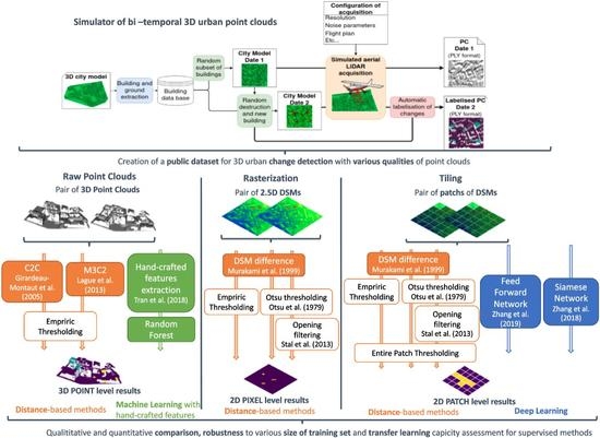
We evaluated a set of methods relying both on extracted DSMs and PCs. The approaches have been selected as representatives of the current literature and are based on distance computation, machine learning with hand-crafted features or deep learning. As shown in the previous section, three levels of outputs are accessible: at the 3D point level, in 2D pixels or in 2D patches. Associated results can be binary (changed/unchanged) or multi-class (unchanged, new construction or destruction).
First, we used DSMd [15], C2C [37] and M3C2 [38] with empirical thresholds, since these basic methods are easy to use and constitute a good baseline. For the DSMd method, we also present results obtained when choosing thresholds with the help of the popular Otsu algorithm [18] and considering a morphological filtering (opening), as suggested in [22], since it allowed us to filter out isolated pixels and to clean up predictions. We also considered the method of Tran et al. [46] as a representative of classical machine learning on hand-crafted features. Finally, even though deep learning methods are a little tougher to experiment with, since training and validation sets need to be constructed, their growing success in remote sensing makes them a must in any benchmark nowadays. Thus, we have implemented the FF CNN and the Siamese CNN architectures of [35,36]. Let us recall that each method has been described in Section 1.2 (for DSM-based ones) or Section 1.3 (for 3D PCs ones). We provide more technical details about methods and experimental settings in the next section. For the Siamese network, we used the architecture proposed in [35] because this study was conducted only on DSMs, as in our study. In their publications, Zhang et al. proposed only binary classification of change. However here, as our dataset contains information on the type of changes, we extended both networks to provide multi-class (MC) classifications of the urban changes. Figure 6 summarizes the methods from the state-of-the-art considered in our comparative study, organized according to their input data types and processing scales.
As far as the metrics are concerned, let us emphasize that the urban change detection problem usually faces the problem of large class imbalance (i.e., most of the 3D points or 2D pixels are unchanged). Thus, the usual overall accuracy or precision is not an appropriate for assessing the performance of a given method. Indeed, a method can reach up to 99% precision even if every pixel or point is predicted as unchanged.
We instead prefer to rely on the mean of intersection over union (IoU) over classes of changes. According to the type of output, it was computed for each pixel, point or patch. In the case of binary classification, this corresponded to the IoU over positive class. Otherwise, for a multi-class scenario, this was the average between the IoU of the new construction class and the IoU of the demolition class.
All methods were tested on each sub-dataset presented in Section 2.2. Thus a first category of tests showed the capabilities of different methods in various contexts: from high resolution with not much noise to low resolution very noisy data as input. Thereby, five tests were carried out for each of the six presented methods. Results are presented in Section 3.1. Then, for machine and deep learning methods, we conducted other tests that considered the size of the training dataset thanks to sub-datasets 1.a, 1.b and 1.c presented in Table 1. Finally, we also aimed to study the behaviors of methods trained on a dataset with a different configuration than the testing set. Thus, for each sub-dataset, we trained machine and deep learning methods before testing them on the other sub-dataset without any re-training process.
2.4. Experimental Settings
C2C and M3C2 were performed with CloudCompare software [50]. We re-implemented feature extraction in Python with all features of [46] except those using LiDAR’s multi-target capability, because our dataset does not contain such information. We observed that some features are very dependent on the neighboring radius size that is chosen. As our datasets had different resolutions than the dataset used in the study of Tran et al., we tested several values of the radius and selected the best value according to each resolution. Thus, for all sub-datasets with the resolution of 0.5 points/m, the radius was fixed to 5 m. For the sub-dataset 2 with a resolution of 10 points/m, a radius of 3 m was selected. Notice that with the multi-sensor sub-dataset 5, the best results were obtained with a radius of 4 m. Training was realized on the training set only.
For deep methods, FF and Siamese network architectures were used similarly to the original papers [35,36]. In their study, Zhang et al. aimed to detect changes between one DSM made from ALS PC data and another one made from photogrammetric data. They presented a few tests with various inputs relying on DSMs only or also on DSMs, and color information coming from RGB orthoimages. Since our dataset only contains information related to the 3D coordinates of points, we kept only configurations where only height information was given. In the case of the FF network, DSMs were provided as inputs through two different channels. For the Siamese network, each DSM was fed into one branch. In our context, the two inputs were quite similar (both were DSMs and came from the same type of sensor); thus, we decided to share weights between the two Siamese branches and to consider a Euclidean distance computation to gather branches, similarly to [35]. When training the deep networks, weight were randomly initialized and all networks were trained from scratch. Batch size was set at 128. For the Siamese network, we used stochastic gradient descent (SGD) with momentum as an optimizer with an initial learning rate of 0.003 and a momentum of 0.9. Unlike [36], we obtained better results with an Adam optimizer with a learning rate of 0.001 for the FF network, so we kept this configuration for the results presented further on. Notice that for both networks, a few tests have been conducted to select the optimal hyper-parameters, i.e., providing the best results on our dataset. The same configurations were kept for all sub-datasets. Implementation was done in Python with PyTorch.
For all methods relying on DSMs as inputs, we used a spatial resolution of 0.3 m. Indeed, as comparisons are made between results obtained on the different sub-datasets presented in Section 2.2. We decided to derive DSM resolution from the PC resolution of sub-dataset 2 (10 points/m). Thus, for all data of lower resolution, interpolation was performed when there was no corresponding points in a given cell (pixel). A coarser resolution could have been chosen, but this would have implied less precise results for 2D pixels and also degraded DSM resolution, which can be obtained with sub-dataset 2. Notice that we ran a test of the DSMd method at a coarser resolution (1.40 m) on sub-dataset 1, but this did not lead to especially better results.
As far as thresholds are considered, we chose -3 and 3 m for MC classification, corresponding to one little floor, since the dataset contains changes from building construction or demolition. The opening filter was using a kernel size. Empiric thresholds for C2C and M3C2 methods varied according to the dataset; we tried several values and systematically selected the best one for each sub-dataset.
In order to derive 2D ground truth from 3D PC labeling, we used a majority voting strategy. Each pixel was given the most frequent label within its corresponding points. When a label was required as the patch scale, we followed the same process as in [36], and marked a patch as changed if the ratio of changed pixels was greater than 10%. For multi-class patch labeling, when a patch was considered as changed, we selected the label according to the majority of pixels in each class of change.
Inspired by [36], patch selection was done with a half-overlap sampling. Classes were largely unbalanced; indeed there were more unchanged areas than changed ones. This imbalance is also visible when looking at the number of patches in each class. We thus relied on data augmentation only for patches of change, as in [36]. A similar kind of data augmentation was applied—namely, vertical and horizontal flips; and rotations with angles of , and . Finally, patches at the edge of the acquisition could contain some empty pixels, since all patches were square but the acquisition area was not. Thus, another threshold was fixed at 90% non-empty pixels to consider a patch as valid. Patch size was set to pixels, corresponding to 30 × 30 m on the ground.
3. Results
We now report the experimental results obtained using the methodology described in Section 2.3 and Section 2.4. First, we assess the performances of the different methods on the different sub-datasets to evaluate their behavior in various acquisition conditions (e.g., resolution, noise, etc). We then study the influence of the training set size and the ability of each method to cope with domain adaptation.
3.1. Experiments on Various PC Acquisition Configurations
Let us recall that results come with different levels depending on the method. All methods dealing with DSMs furnished results in 2D. First, DSMd led to the per-2D-pixel results presented in Table 2. This table summarizes results for all sub-datasets with different ways of selecting thresholds (via an empirical choice or Otsu algorithm, as mentioned in the previous section). It also contains the results of the DSMd method with an opening operation and the Otsu algorithm. For each sub-dataset and type of classification (binary or MC), bold results indicate the best performing methods for this scenario. Following these quantitative results, Figure 7, Figure 8, Figure 9, Figure 10 and Figure 11 give a zoomed view of the testing set for each of the five sub-datasets. These figures contain DSMs extracted from original PCs, the 2D corresponding ground truth and the results for the three versions of DSMd. We also provide each result with an error map (g,h,i). One can notice the difference in terms of quality of DSMs among different sub-datasets. In particular, Figure 8a,b and Figure 11b correspond to DSMs of high resolution with low-noise PCs. DSMs of Figure 7a,b corresponding to low resolution but not noisy ALS data (sub-dataset 1.b) are a touch less precise. Finally, Figure 9a,b, Figure 10a,b and Figure 11a were extracted from low resolution and noisy PCs, and thereby they seem more inaccurate and blurry.
While the initial results with empirical thresholding are not convincing, we can see that a significant improvement occurred when using the Otsu algorithm to select thresholds (values of about −9 and 9 m). The results were further improved when an opening filter was added to remove isolated pixels that do not correspond to real changes. Visual assessment confirmed the utility of the opening filter (f–i) compared to the initial results with empirically-set thresholds (d–g) or using the Otsu algorithm (e–h), and its ability to remove isolated pixels (Figure 7, Figure 8, Figure 9, Figure 10 and Figure 11). Unsurprisingly, the best results were achieved on the second sub-dataset corresponding to pairs of PCs with high resolution and a low level of noise. Notice that the gap in quality between DSMd with a filtering operation and DSMd with the Otsu algorithm was higher for sub-datasets containing noisy data (sub-datasets 3, 4 and 5). Indeed, Table 2 reports a gain of about 12 points of mean of IoU between DSMd+Otsu and DSMd+Otsu+Opening methods for sub-datasets 1.b and 2 with low levels of noise, whereas the opening filter increased this metric by 17–22 points for datasets that contain noisy PCs. Indeed, noisy data led to numerous false detection instances in isolated parts of the DSM, which could be eliminated through this morphological operation. This is visible in Figure 9d–g and Figure 10d–g, where isolated pixels marked as new construction or demolition can be seen. In addition to these isolated pixels, almost all building edges were brought out with empirical thresholds in particular, because of the noise on vertical facades especially disturbing the DSM extraction. Indeed, such noise makes the facade not straight and difficult to distinguish precisely from an above point of view, as highlighted in sub-datasets 3, 4 and 5 (Figure 9, Figure 10 and Figure 11). Notice that with Otsu thresholding, it remained visible (at a lower level though).
When looking at Table 2, one can notice that even if the worst results were obtained for sub-datasets 3 and 5 without the filtering operation, the scores became comparable with sub-dataset 1.b when adding the filtering step. Thus, even in cases of noisy data (for one or both PCs), we could achieve similar performance as with a low-noise setup thanks to the morphological operation. However results in the multi-sensor scenario (sub-dataset 5) remained lower than with sub-dataset 2, even though one of the PCs of sub-dataset 5 has the same quality as sub-dataset 2. A visual assessment of the effects brought about by the opening operation on sub-datasets 3 and 5 (Figure 9f–i and Figure 11f–i) shows quite similar results. True changes are visible, but there are still quite a few instances of false change detection.
Surprisingly, the fourth sub-dataset obtained a high mean of IoU on classes of change according to Table 2. This is particularly visible for DSMd with the Otsu algorithm and the opening filter. This sub-dataset is composed of a pair of PCs with low resolution (0.5 points/m) and high noise, sub-dataset 3. However, the range of scanning angles during acquisition and the overlap between flight tracks were both halved; see Table 1. Using this configuration, we aimed to mimic photogrammetric PCs acquired thanks to satellite images. These images have a top-down point of view, leading to fewer shadows. Indeed, the higher the scanning angle and the higher the building, the more shadows in the PCs. In the context of DSM extraction, a building shadow implies empty pixels. In this study, we filled them through interpolation, but this may lead to errors or at least a lack of precision in these areas. Moreover, the flight plan was not the same for the acquisitions of the pair of PCs; hence, shadows are not the same in each PC. Thus, high difference values can be obtained even in unchanged areas. For a qualitative illustration, refer to Figure 8d–e, where a band of pixels marked as changed is always visible on the same side of every building. Indeed, we can also see the difference in DSMs: the north sides of buildings seem more blurry than the other sides in DSM 1 (Figure 8a), due to a lack of information in the area just near the facade because of building shadows. In comparison, as the flight plan was not the same for DSM 2 (Figure 8b), building edges are more distinct at the bottom of the image. Some mis-classifications could be corrected by the opening filter, but only up to a certain extent (i.e., not the larger ones). Finally, sub-dataset 4 contains fewer building shadows, leading to easier identification of true changes. This explains the higher results achieved on this photogrammetric, look-alike sub-dataset 4 and reported in Table 2. Notice that building edges were also brought out in Figure 10d–e because of the noisiness of the photogrammetric, look-alike sub-dataset 4. This differs from sub-dataset 3, where both effects are visible on buildings’ edges: some edges are continuous in one class of change corresponding to building shadows, and predictions of other edges are more heterogeneous. Notice that heterogeneous parts are easily cleaned with the opening operation, leading to a significant difference of results between sub-datasets 3 and 4 in Table 2.
Table 3 presents results at the 2D patch level for deep learning methods. When comparing both FF and Siamese networks, we can see that better results were obtained with the FF architecture. The same trend was reported in [36] for when only DSM information was given to the networks. However, in these original works [35,36], results were only binary. We propose here to extend these approaches to deal with MC classification. For FF architectures, the quality of MC results is close to the binary case, with only 3–5 points less, depending on the sub-dataset. On the contrary, the Siamese architecture leads to a higher gap, with a 7–10% loss between binary and MC classification. Thereby, Siamese architecture seems less efficient in this context. Better results were again obtained for the high resolution sub-dataset 2; they were rather similar for sub-datasets 1.b, 3 and 5. Here again, identification of true changed patches seemed to be easier for sub-dataset 4, which showed better results than sub-datasets 1.b, 3 and 5.
For the sake of comparison, we have adapted at the patch level the DSMd method and its variant, i.e., considering Otsu thresholding and morphological filtering. To do so, we have followed the patch-wise strategy introduced in previous works and reported in Section 2.4. Namely, we divided with half-overlap sampling the different DSMd results into patches in order to extract same patches as those that are extracted for deep learning methods. To retrieve labels at patch level, we set a threshold on the percentage of changed pixels according to each DSMd results. For MC classification, when a patch was identified as changed, we have the label of the most prominent class of change. Thresholds of validity and changed pixels were set accordingly to the setup used with deep learning methods (90% and 10%, respectively). Results are given in Table 3. We can see that DSMd with the Otsu algorithm and opening filter overtook deep methods for all sub-datasets. Let us note that the coarseness of the analysis (patch instead of pixel) hinders the interest of a visual assessment.
Finally, Table 4 gives results at the 3D point level. Notice that the C2C method provides unsigned results, which makes impossible the distinction between positive and negative changes; thus, only binary results are provided. Here again, one method surpassed the others for each kind of sub-dataset. Indeed, the machine learning method of [46], using the RF algorithm trained on hand-crafted features with a stability feature, had more precise results. Notice that M3C2 did not seem to have interesting results in the context of quite low resolution PCs: the means of IoU for classes of change were higher than 50% only for the sub-dataset with the higher resolution. As far as binary results are concerned, C2C seems more suitable if no labeled training set is available. The RF algorithm with hand-crafted features have quite similar results for binary and MC classification. Let us emphasize that Tran et al. [46] designed their method and especially the feature extraction for a MC classification scenario.
For the sake of qualitative assessment at the 3D point level, Figure 12 and Figure 13 provide PCs for both dates; the associated ground truth according to the change; and the results provided by C2C, M3C2 and the RF method with hand-crafted features. Firstly, one should remark on the difference of quality between all sub-datasets. Indeed, Figure 12a,b presents low-noise PCs at low resolution, (a) corresponding to the first sub-dataset, and high resolution, (b) corresponding to the second sub-dataset. On the other hand, Figure 13a–c shows PCs of noisy sub-datasets. In Figure 13c, the difference between the noisy, low-resolution PC and the precise, high-resolution PC is substantial.
As far as quantitative results are concerned, the same tendency is visible in Table 4. C2C binary results do not seem so far from ground truth in changed areas; however, it led to some false positive predictions on building facades. M3C2 led to even more false positives, but also it did not highlight changes in some areas. This is particularly visible in Figure 12b, where a lot of points lying on unchanged facades are identified as changed, conversely to points on the facade of the new building. Moreover, in the same example, some points were even identified as destruction instead of construction. For all sub-datasets, the RF method [46] seemed to bring quite accurate results, except for the ground points near buildings; those points were identified as deconstructed. This is visible in Figure 12a and Figure 13a,c, corresponding to the building shadow effects already mentioned. When looking directly at the PCs of both dates, it is particularly visible in Figure 12a that all points assigned a deconstruction label at ground level, which are not true deconstruction, are points that do not exist in the first PC (PC 1).
Notice that no confusion between the two classes of change seems to have arisen in the RF method. More specifically, this method seems to have learned that deconstruction is always at ground level; this is not the case for the M3C2 method. Indeed, since only thresholding was applied, some deconstruction parts could appear on facades. Finally, point predictions on roofs were not so far from ground truth for all methods, though M3C2 results were the least accurate.
3.2. Experiments with Various Training Configurations
Having quantitatively and qualitatively assessed the performances of the different methods when applied to various acquisition conditions, as demonstrated in our pool of sub-datasets, we now focus on the generalization capacities of supervised methods. We especially study their behaviors when trained on datasets of various sizes or having different characteristics. Indeed, most often, no annotated data are available for the target areas, and/or such areas are not covered by the same sensors (or the same acquisition conditions) as the training areas. Thus, it is crucial to assess the ability of techniques trained on synthetic data to perform on various datasets.
Table 5 helps us to study the influence of the training set size. Indeed, the three sub-datasets were of similar type (ALS with low resolution and low noise); the difference lay in the size of the set by varying the number of pairs of simulated PCs (1, 10 and 50). Note that the validation set was the same for the three tests. Unsurprisingly, the best results were obtained with the largest training set (1.c), which is consistent with common observations using neural networks or RF. However, in the latter case using hand-crafted features, the improvement was limited compared with the case of a neural network: a bit less than using RF between sub-datasets 1.a and 1.c, compared to and with FF method (binary and MC) and ≈ and with Siamese network (binary and MC), respectively. One can notice that for the smallest training set (1.a), the Siamese network led to better binary results than the FF network. Contrary to the RF method, the gap between sub-datasets 1.a and 1.b was larger than between sub-datasets 1.b and 1.c.
Finally, one can notice that DSMd with the Otsu thresholding and opening filtering was still a bit better than deep networks at the 2D patch level trained on the larger dataset (see Table 3).
Figure 14 provides clues to assess the transfer capacity, through training (and validating) on a dataset with different characteristics than the testing set. Here we consider each transfer learning scenario with various training configurations related to all five sub-datasets discussed above. Notice that the trained models were directly applied to the testing set, without re-training. In each line of Figure 14, the “star” corresponds to the scenario where training and test sets were similar, i.e., without transfer learning (and this can be seen as the reference). Let us recall that with these methods, those based on neural networks led to results on patches, whereas RF methods led to results on PCs. Thus a direct comparison between deep learning and the RF methods is not directly possible. It is, however, still interesting to outline that the RF method with hand-crafted features seems to be the more impacted by the nature of training sets. Depending on the configurations of training and testing sets, great variability in terms of results can be observed. For example, when transferring from a noisy photogrammetric type of PC (sub-dataset 4) to noise-free ALS data (sub-dataset 1, 2) or multi-sensor data (sub-dataset 5), results go down from 68.87% for the reference test to, respectively, 31.43%, 9.56% and 5.1% when transferring to sub-dataset 1, 2 and 5; see Figure 14d. As expected, the more different the data, the more the RF method struggles to retrieve changes. Indeed, both noisy datasets (sub-datasets 3 and 4) produced similar outcomes. When looking at Figure 14b, it is worth noting that the results of tests on the multi-sensor sub-dataset are nearly equivalent to the reference test results corresponding to tests on high-resolution ALS data. Indeed, the second part of the multi-sensor sub-dataset has a similar configuration to sub-dataset 2. Thus, the extracted hand-crafted features should have been quite similar. However, as can be seen in Figure 14e, a larger difference of results came about when training on sub-dataset 5 and testing on sub-dataset 2. Finally, let us outline that training on sub-dataset 1 leds to a lower difference among results when transferring to another sub-dataset (Figure 14a). Sub-dataset 1 has the same resolution as sub-datasets 3 and 4, and the first instance of the sub-dataset 5, but is not noisy like sub-dataset 2 and the second instance of the sub-dataset 5.
As far as deep neural methods are concerned, results on transfer learning are quite similar to those obtained without transfer leaning. However, the Siamese architecture seems to be more affected by the transfer learning scenario considering training on the multi-sensor dataset and testing on the other sub-dataset. Let us also notice that results that resulted from transferring to the sub-dataset 4 are often lower. In this case, as seen in Section 3.1, the characteristics of sub-dataset 4 differ significantly from those of the others, since it corresponds to a photogrammetry-like scenario. Even if change detection on DSMs seems easier for sub-dataset 4 (see results in Table 2 and Table 3), the very different characteristics with respect to the other sub-datasets used for the test made these transfer learning scenarios achieve lower results. More generally, we can observe deep neural network approaches exhibited relatively good generalization properties. This is very encouraging, since one can easily learn on simulated data to classify changes in real PCs. Conversely, when considering the RF method with hand-crafted features [46], it seems better to train on a smaller dataset than on datasets with different characteristics.
4. Discussion
Complementarily to the experimental results presented in the previous section, we provide here an in-depth discussion addressing the change detection methods, the dataset used in this study and the simulation tool that has been employed.
4.1. Methods
In this study, we have compared methods producing results at different levels on various kinds of 3D change datasets. As far as the DSMd method is concerned, even if the Otsu thresholding substantially improves the results, we observed than changes below 9 m cannot be retrieved. Even if such a situation rarely occurs in our datasets, it could still be problematic in practice, e.g., in low residential zones. One example of low building changes better retrieved with empirical thresholds (set at −3 and 3 m) can be seen in Figure 11.
While deep learning have been shown to generally surpass traditional ones in remote sensing, this tendency was not confirmed in our study. Indeed, existing deep learning methods for 3D change detection only give patchwise results, leading to no fine change object boundaries [43]. The best results obtained at 2D patch level were those provided by the traditional DSMd coupled Otsu thresholding and the opening filter. Zhang et al. [36] also compared their results on DSMd at the 2D patch level, but they assigned a label to each patch of DSMd according to the average height difference (AHD) in the patch. Conversely, we first extracted labels at the pixel level before applying majority vote filtering to produce results at the patch level. For the sake of comparison, we have also computed patch labels based on AHD, leading to the same results as those obtained by the majority voting procedure. In addition, Zhang et al. also applied the Otsu thresholding algorithm, but they did not consider a morphological operation to filter out isolated pixels. One other non-negligible difference from our study is that our dataset does not contain vegetation. In such a simple situation, the DSMd method enhanced with a filtering operation and a selection of adequate thresholds with the Otsu algorithm would lead to satisfying results. One can assume the deep networks also benefited from this simpler setup.
Let us recall that Zhang et al. reported in the binary case an IoU over the class of change of 67% [35]. However, a direct comparison with our results is not possible, since our dataset is different. Still, it is worth noting that quantitative results showed similar ranges. Similarly to [35], we used a Siamese network with shared weight as both input data or DSMs. This was also the case for sub-dataset 5 on multi-sensor data, even through the two PCs (from which DSMs have been extracted) have different characteristics. Notice that for this multi-sensor sub-dataset, we also tried a pseudo-Siamese network with unshared weights, as is commonly done when inputs have dissimilarities [34,51], even if both inputs remain DSMs. We did not observe convincing results, probably because the pseudo-Siamese networks come with higher complexity (more parameters), thereby requiring larger training sets.
When focusing on methods dealing directly with the raw PCs, we observed a huge gap between traditional approaches and machine learning-based ones. However, one should notice that C2C and M3C2 methods were not especially designed for urban change detection. More particularly, M3C2 was presented in a study using TLS PCs with tremendously higher resolution than ours. While [38] sought changes at the centimetric scale within PCs of millimetric resolution (point spacing was about 10 mm horizontally and 5 mm vertically) acquired at a distance of 50 m, our point spacing in sub-dataset 2 with the higher resolution was about 20 to 30 cm, and we focused on changes on a metric scale. Their method is thus possibly inadequate for our settings. Both C2C and M3C2 are very sensitive, and the optimal thresholds are specific to each dataset (conversely to DSMd, where the threshold value is the same for all datasets). Automatic threshold selection, thanks to the Otsu algorithm, did not lead to satisfying results.
4.2. Dataset
Our experimental results allowed us to compare different methods on a same dataset and in different conditions. We have also highlighted inherent difficulties of each kind of sub-dataset. The first sub-dataset has a low resolution, and although it embeds low noise, it contains lots of building shadows and hidden facades due to the acquisition settings. Therefore, both PCs do not contain the same hidden parts and building shadows, making a direct comparison difficult. The second sub-dataset with high resolution and low noise seems to be the easiest one for change detection and characterization. Indeed, all methods performed best on this sub-dataset. The third sub-dataset is composed of PCs with low resolution and high noise, and includes some shadows due to the different flight tracks of LiDAR during the acquisition of both PCs. This sub-dataset generally led to results worse than with the fourth sub-dataset, which is also composed of low-resolution, noisy PCs, but with a lower scanning angle, leading to less shadows and to more similar hidden parts between PCs. As already discussed in the previous section, it had a significant impact on all change detection methods. With this fourth sub-dataset, we aimed to mimic photogrammetric PCs extracted from satellites images. A possibility to enhance the realism would be to adapt the registration error brought about by the acquisition sensor [52], but this remains quite specific to each sensor. Finally, the fifth sub-dataset is composed of multi-sensor data: the first PC is from a low-resolution, noisy ALS, and the second PC has a high resolution and low noise. Results achieved on this multi-sensor sub-dataset are similar to those obtained on the first sub-dataset composed of low resolution but not noisy PCs.
Completion of all experiments led us to conclude that resolution seems to have more of an impact than noise on the final results. However, since changes in the dataset occurred at building scale (new construction or destruction) and noise was set to be about 1 m, it seems rational that the main changes were retrieved. The main difficulties remain at the buildings’ edges, since in this situation, noise makes it difficult to distinct boundaries of changed objects.
Finally, even though the proposed dataset may appear too simple because it only contains ground and buildings, results show that there are some difficulties in dealing with dense urban areas where building shadows and hidden parts are frequent. These shadows and hidden parts are frequent in real 3D data and greatly challenge the comparison between two point clouds [53]. Moreover, one can observe that, even for the sub-dataset with high resolution and low noise, all methods were still far from attaining 100% for their means of IoU over classes of change. Indeed, the best methods obtained about 80% at the 2D pixel level, 90% at the 2D patch level and 70% at the 3D point level. Thereby, this calls for new change detection and characterization methods, and indicates as well the possible difficulties future methods need to surpass with our dataset.
4.3. Simulation
Let us recall that our dataset is made of artificial PCs generated thanks to a novel simulator of multi-temporal 3D urban PCs. The annotation is done automatically by the simulator, thus avoiding any time-consuming manual annotation. The new construction label corresponds to all points located on a new building. For the demolition class of change, we proceeded by extracting the convex hull of the building footprint on the ground. In our 3D models, the majority of buildings are convex, but in some isolated cases this could lead to some small difference with the actual building footprints. Nevertheless, such a case remains very rare with respect to the large number of annotated points, so it does not have a significant influence on the quantitative results that have been reported.
Results presented in Section 3.2 concerning the size of the training set also show some additional interest of our simulator. Indeed, up to 50 simulations of PC pairs have been performed in order to generate the larger sub-dataset 1.c. All these simulations have been made over the same area but, for each generated PC, we randomly selected both the buildings to be updated and the flight tracks to be followed, thus leading to a high variability in the dataset, as illustrated in Figure 3. Though each simulated pair may not be considered as a totally new data (since similar buildings could be randomly chosen several times), this process can be seen as data augmentation, allowing us to significantly increase the results, as shown in previous section (e.g., up to 24% for the binary FF network between the smaller (1.a) and the larger (1.c) sub-dataset). Finally, it should be noted that even if the same buildings can be randomly chosen several times, the resulting 3D points lying on the building will not be at the exact same coordinates because of the random flight plan and noise.
5. Conclusions
In this study, we aimed to propose an experimental comparison of different methods of change detection and characterization in a urban environment. To do so, we especially designed a dataset consisting of pairs of 3D PCs that were annotated according to the changes occurring in urban areas. This dataset has been acquired thanks to our original simulator of multi-temporal urban models, where 3D PC acquisition is simulated by mimicking airborne LiDAR surveying. This simulator allowed us to acquire various pairs of annotated PCs and to further train supervised methods. Moreover, we were able to generate five different sub-datasets with various acquisition configurations illustrating the variability in terms of sensor quality and type as faced in real 3D PC acquisition. For one of the sub-datasets, we also considered several training set sizes to assess the robustness of the methods with respect to several training configurations. The dataset composed of all its sub-datasets is publicly available (it is available at the following link https://ieee-dataport.org/open-access/urb3dcd-urban-point-clouds-simulated-dataset-3d-change-detection, accessed on 7 May 2021) to support reproducible research and to foster further works on 3D change detection, especially with deep learning methods. On all these sub-datasets, we have experimented and assessed six different methods for change detection and characterization using either PC rasterizations in 2D DSMs, or by directly coping with the 3D PCs. More precisely, we have compared traditional methods such as DSMd with different types of thresholding and a filtering operation [15,18,22], C2C [37] and M3C2 [38]; with a machine learning technique, a random forest fed with hand-crafted features [46]; and with deep learning architectures through feed forward [36] and Siamese [35] networks. These methods provide different results: 2D pixels, 2D patches and 3D points. For the supervised methods, we have also studied the capacity of transfer learning and the influence of the training set size.
Assessment of the benchmark results showed that our dataset simulated over dense urban areas is actually challenging for all existing methods, even though it contains changes at only the building level. Remaining issues concern the handling of low resolutions and the global scene understanding when dealing with hidden parts in the PCs. As a matter of fact, the best results at the 3D point level were obtained with traditional machine learning with hand-crafted features with an IoU over classes of 70.12% in a noise-free high resolution context, and 58.83% for noisy and low resolution ALS PCs. Then, even though deep learning methods seem to be more suitable for transfer learning purposes, these experiments exhibited the need for deep learning methods that process raw 3D PCs for change detection. Moreover, the existing deep networks on patches of DSM did not show astonishing results since the filtered and thresholded DSMd led to better results (from 2% to 17% depending on the deep network architecture and the conditions of acquisition of the dataset). Thereby, our future work will focus on developing original 3D change detection and characterization methods able to understand the 3D context even at a low resolution and in noisy conditions. We also plan to improve our simulator in order to generate even more realistic PCs by integrating vegetation and other type of changes.
Author Contributions
Conceptualization, I.d.G., S.L. and T.C.; methodology, I.d.G.; software, I.d.G.; validation, I.d.G.; formal analysis, I.d.G.; investigation, I.d.G.; writing—original draft preparation, I.d.G.; writing—review and editing, I.d.G., S.L. and T.C.; supervision, S.L. and T.C.; project administration, S.L. and T.C.; funding acquisition, S.L. and T.C. All authors have read and agreed to the published version of the manuscript.
Funding
This research was funded by Magellium, Toulouse and the CNES, Toulouse.
Institutional Review Board Statement
Not applicable.
Informed Consent Statement
Not applicable.
Data Availability Statement
Dataset is made publicly available on IEEE Dataport at the following link https://ieee-dataport.org/open-access/urb3dcd-urban-point-clouds-simulated-dataset-3d-change-detection, accessed on 7 May 2021.
Conflicts of Interest
The authors declare no conflict of interest. The funders had no role in the design of the study; in the collection, analyses, or interpretation of data; in the writing of the manuscript, or in the decision to publish the results.
Abbreviations
The following abbreviations are used in this manuscript:
| ALS | Aerial Laser Scanning |
| C2C | Cloud to Cloud |
| CPU | Central Processing Unit |
| CNN | Convolutional Neural Network |
| DSM | Digital Surface Model |
| DSMd | DSM difference |
| DTM | Digital Terrain Model |
| FF | Feed Forward |
| GT | Ground Truth |
| IoU | Intersection over Union |
| LoD2 | Level of Detail 2 |
| LiDAR | Light Detection And Ranging |
| MC | Multi-Class |
| M3C2 | Multi-Scale Model to Model Cloud Comparison |
| PC | Point Cloud |
| RANSAC | Random Sample Consensus |
| RF | Random Forest |
| RGB | Red Green Blue |
| SAR | Synthetic Aperture Radar |
| VTK | Visualisation ToolKit |
| 2D | 2-Dimensional |
| 3D | 3-Dimensional |
References
- Rottensteiner, F. Automated Updating of Building Data Bases from Digital Surface Models and Multi-Spectral Images: Potential and Limitations; ISPRS Congress: Beijing, China, 2008; Volume 37, pp. 265–270. [Google Scholar]
- Champion, N.; Boldo, D.; Pierrot-Deseilligny, M.; Stamon, G. 2D building change detection from high resolution satelliteimagery: A two-step hierarchical method based on 3D invariant primitives. Pattern Recognit. Lett. 2010, 31, 1138–1147. [Google Scholar] [CrossRef]
- Rahman, M.T. Detection of land use/land cover changes and urban sprawl in Al-Khobar, Saudi Arabia: An analysis of multi-temporal remote sensing data. ISPRS Int. J. Geo-Inf. 2016, 5, 15. [Google Scholar] [CrossRef]
- Reynolds, R.; Liang, L.; Li, X.; Dennis, J. Monitoring annual urban changes in a rapidly growing portion of northwest Arkansas with a 20-year Landsat record. Remote Sens. 2017, 9, 71. [Google Scholar] [CrossRef] [Green Version]
- Sofina, N.; Ehlers, M. Building change detection using high resolution remotely sensed data and GIS. IEEE J. Sel. Top. Appl. Earth Obs. Remote Sens. 2016, 9, 3430–3438. [Google Scholar] [CrossRef]
- Vetrivel, A.; Gerke, M.; Kerle, N.; Nex, F.; Vosselman, G. Disaster damage detection through synergistic use of deep learning and 3D point cloud features derived from very high resolution oblique aerial images, and multiple-kernel-learning. ISPRS J. Photogramm. Remote Sens. 2018, 140, 45–59. [Google Scholar] [CrossRef]
- Si Salah, H.; Ait-Aoudia, S.; Rezgui, A.; Goldin, S.E. Change detection in urban areas from remote sensing data: A multidimensional classification scheme. Int. J. Remote Sens. 2019, 40, 6635–6679. [Google Scholar] [CrossRef]
- Lu, D.; Mausel, P.; Brondizio, E.; Moran, E. Change detection techniques. Int. J. Remote Sens. 2004, 25, 2365–2401. [Google Scholar] [CrossRef]
- Shi, W.; Zhang, M.; Zhang, R.; Chen, S.; Zhan, Z. Change detection based on artificial intelligence: State-of-the-art and challenges. Remote Sens. 2020, 12, 1688. [Google Scholar] [CrossRef]
- Qin, R.; Tian, J.; Reinartz, P. 3D change detection—Approaches and applications. P&RS 2016, 122, 41–56. [Google Scholar]
- Amini Amirkolaee, H.; Arefi, H. 3D change detection in urban areas based on DCNN using a single image. Int. Arch. Photogramm. Remote Sens. Spat. Inf. Sci. 2019, XLII-4/W18, 89–95. [Google Scholar] [CrossRef] [Green Version]
- Waser, L.; Baltsavias, E.; Eisenbeiss, H.; Ginzler, C.; Grün, A.; Kuechler, M.; Thee, P. Change detection in mire ecosystems: Assessing changes of forest area using airborne remote sensing data. Int. Arch. Photogramm. Remote Sens. Spat. Inf. Sci. 2007, 36, 313–318. [Google Scholar]
- Guerin, C.; Binet, R.; Pierrot-Deseilligny, M. Automatic detection of elevation changes by differential DSM analysis: Application to urban areas. IEEE J. Sel. Top. Appl. Earth Obs. Remote Sens. 2014, 7, 4020–4037. [Google Scholar] [CrossRef]
- Erdogan, M.; Yilmaz, A. Detection of building damage caused by Van Earthquake using image and Digital Surface Model (DSM) difference. Int. J. Remote Sens. 2019, 40, 3772–3786. [Google Scholar] [CrossRef]
- Murakami, H.; Nakagawa, K.; Hasegawa, H.; Shibata, T.; Iwanami, E. Change detection of buildings using an airborne laser scanner. P&RS 1999, 54, 148–152. [Google Scholar]
- Okyay, U.; Telling, J.; Glennie, C.; Dietrich, W. Airborne lidar change detection: An overview of Earth sciences applications. Earth-Sci. Rev. 2019, 198, 102929. [Google Scholar] [CrossRef]
- Vu, T.T.; Matsuoka, M.; Yamazaki, F. LIDAR-based change detection of buildings in dense urban areas. In Proceedings of the IGARSS 2004, 2004 IEEE International Geoscience and Remote Sensing Symposium, Anchorage, AK, USA, 20–24 September 2004; Volume 5, pp. 3413–3416. [Google Scholar]
- Otsu, N. A threshold selection method from gray-level histograms. IEEE Trans. Syst. Man Cybern. 1979, 9, 62–66. [Google Scholar] [CrossRef] [Green Version]
- Gharibbafghi, Z.; Tian, J.; Reinartz, P. Superpixel-Based 3D Building Model Refinement and Change Detection, Using VHR Stereo Satellite Imagery. In Proceedings of the IEEE/CVF Conference on Computer Vision and Pattern Recognition Workshops, Long Beach, CA, USA, 16–17 June 2019. [Google Scholar]
- Choi, K.; Lee, I.; Kim, S. A feature based approach to automatic change detection from LiDAR data in urban areas. Int. Arch. Photogramm. Remote Sens. Spat. Inf. Sci. 2009, 18, 259–264. [Google Scholar]
- Dini, G.; Jacobsen, K.; Rottensteiner, F.; Al Rajhi, M.; Heipke, C. 3D building change detection using high resolution stereo images and a GIS database. Int. Arch. Photogramm. Remote Sens. Spat. Inf. Sci. ISPRS Arch. 2012, 39, 299–304. [Google Scholar] [CrossRef] [Green Version]
- Stal, C.; Tack, F.; De Maeyer, P.; De Wulf, A.; Goossens, R. Airborne photogrammetry and lidar for DSM extraction and 3D change detection over an urban area–a comparative study. Int. J. Remote Sens. 2013, 34, 1087–1110. [Google Scholar] [CrossRef] [Green Version]
- Teo, T.A.; Shih, T.Y. Lidar-based change detection and change-type determination in urban areas. Int. J. Remote Sens. 2013, 34, 968–981. [Google Scholar] [CrossRef]
- Pang, S.; Hu, X.; Wang, Z.; Lu, Y. Object-based analysis of airborne LiDAR data for building change detection. Remote Sens. 2014, 6, 10733–10749. [Google Scholar] [CrossRef] [Green Version]
- Lyu, X.; Hao, M.; Shi, W. Building Change Detection Using a Shape Context Similarity Model for LiDAR Data. ISPRS Int. J. Geo-Inf. 2020, 9, 678. [Google Scholar] [CrossRef]
- Peng, D.; Zhang, Y. Building change detection by combining Lidar data and ortho image. Int. Arch. Photogramm. Remote Sens. Spat. Inf. Sci. 2016, 41, 669–676. [Google Scholar] [CrossRef] [Green Version]
- Wang, X.; Li, P. Extraction of urban building damage using spectral, height and corner information from VHR satellite images and airborne LiDAR data. ISPRS J. Photogramm. Remote Sens. 2020, 159, 322–336. [Google Scholar] [CrossRef]
- Warth, G.; Braun, A.; Bödinger, C.; Hochschild, V.; Bachofer, F. DSM-based identification of changes in highly dynamic urban agglomerations. Eur. J. Remote Sens. 2019, 52, 322–334. [Google Scholar] [CrossRef] [Green Version]
- Jang, Y.J.; Oh, K.Y.; Lee, K.J.; Oh, J.H. A study on urban change detection using D-DSM from stereo satellite data. J. Korean Soc. Surv. Geod. Photogramm. Cartogr. 2019, 37, 389–395. [Google Scholar]
- Kalantar, B.; Ueda, N.; Al-Najjar, H.A.; Halin, A.A. Assessment of Convolutional Neural Network Architectures for Earthquake-Induced Building Damage Detection based on Pre-and Post-Event Orthophoto Images. Remote Sens. 2020, 12, 3529. [Google Scholar] [CrossRef]
- Zhan, Y.; Fu, K.; Yan, M.; Sun, X.; Wang, H.; Qiu, X. Change detection based on deep siamese convolutional network for optical aerial images. IEEE Geosci. Remote Sens. Lett. 2017, 14, 1845–1849. [Google Scholar] [CrossRef]
- Lefèvre, S.; Tuia, D.; Wegner, J.D.; Produit, T.; Nassar, A.S. Toward seamless multiview scene analysis from satellite to street level. Proc. IEEE 2017, 105, 1884–1899. [Google Scholar] [CrossRef] [Green Version]
- He, H.; Chen, M.; Chen, T.; Li, D. Matching of remote sensing images with complex background variations via Siamese convolutional neural network. Remote Sens. 2018, 10, 355. [Google Scholar] [CrossRef] [Green Version]
- Mou, L.; Schmitt, M.; Wang, Y.; Zhu, X.X. A CNN for the identification of corresponding patches in SAR and optical imagery of urban scenes. In Proceedings of the 2017 Joint Urban Remote Sensing Event (JURSE), Dubai, United Arab Emirates, 6–8 March 2017; pp. 1–4. [Google Scholar]
- Zhang, Z.; Vosselman, G.; Gerke, M.; Tuia, D.; Yang, M.Y. Change detection between multimodal remote sensing data using siamese CNN. arXiv 2018, arXiv:1807.09562. [Google Scholar]
- Zhang, Z.; Vosselman, G.; Gerke, M.; Persello, C.; Tuia, D.; Yang, M. Detecting building changes between airborne laser scanning and photogrammetric data. Remote Sens. 2019, 11, 2417. [Google Scholar] [CrossRef] [Green Version]
- Girardeau-Montaut, D.; Roux, M.; Marc, R.; Thibault, G. Change detection on points cloud data acquired with a ground laser scanner. ISPRS Arch. 2005, 36, 30–35. [Google Scholar]
- Lague, D.; Brodu, N.; Leroux, J. Accurate 3D comparison of complex topography with terrestrial laser scanner: Application to the Rangitikei canyon (NZ). P&RS 2013, 82, 10–26. [Google Scholar]
- Shirowzhan, S.; Sepasgozar, S.; Li, H.; Trinder, J.; Tang, P. Comparative analysis of machine learning and point-based algorithms for detecting 3D changes in buildings over time using bi-temporal lidar data. Autom. Constr. 2019, 105, 102841. [Google Scholar] [CrossRef]
- Awrangjeb, M.; Fraser, C.; Lu, G. Building change detection from LiDAR point cloud data based on connected component analysis. ISPRS Ann. Photogramm. Remote Sens. Spat. Inf. Sci. 2015, 2, 393. [Google Scholar] [CrossRef] [Green Version]
- Siddiqui, F.U.; Awrangjeb, M. A novel building change detection method using 3d building models. In Proceedings of the 2017 International Conference on Digital Image Computing: Techniques and Applications (DICTA), Sydney, Australia, 29 November–1 December 2017; pp. 1–8. [Google Scholar]
- Xu, S.; Vosselman, G.; Oude Elberink, S. Detection and classification of changes in buildings from airborne laser scanning data. Remote Sens. 2015, 7, 17051–17076. [Google Scholar] [CrossRef] [Green Version]
- Dai, C.; Zhang, Z.; Lin, D. An Object-Based Bidirectional Method for Integrated Building Extraction and Change Detection between Multimodal Point Clouds. Remote Sens. 2020, 12, 1680. [Google Scholar] [CrossRef]
- Roynard, X.; Deschaud, J.E.; Goulette, F. Fast and robust segmentation and classification for change detection in urban point clouds. ISPRS Arch. 2016, XLI-B3, 693–699. [Google Scholar]
- Xu, H.; Cheng, L.; Li, M.; Chen, Y.; Zhong, L. Using octrees to detect changes to buildings and trees in the urban environment from airborne LiDAR data. Remote Sens. 2015, 7, 9682–9704. [Google Scholar] [CrossRef] [Green Version]
- Tran, T.; Ressl, C.; Pfeifer, N. Integrated change detection and classification in urban areas based on airborne laser scanning point clouds. Sensors 2018, 18, 448. [Google Scholar] [CrossRef] [PubMed] [Green Version]
- Zhu, X.X.; Tuia, D.; Mou, L.; Xia, G.S.; Zhang, L.; Xu, F.; Fraundorfer, F. Deep learning in remote sensing: A comprehensive review and list of resources. IEEE Geosci. Remote Sens. Mag. 2017, 5, 8–36. [Google Scholar] [CrossRef] [Green Version]
- Ma, L.; Liu, Y.; Zhang, X.; Ye, Y.; Yin, G.; Johnson, B.A. Deep learning in remote sensing applications: A meta-analysis and review. ISPRS J. Photogramm. Remote Sens. 2019, 152, 166–177. [Google Scholar] [CrossRef]
- de Gélis, I.; Lefèvre, S.; Corpetti, T.; Ristorcelli, T.; Thénoz, C.; Lassalle, P. Benchmarking change detection in urban 3D point clouds. In Proceedings of the IEEE International Geoscience and Remote Sensing Symposium (IGARSS), Brussels, Belgium, 11–16 July 2021. [Google Scholar]
- Girardeau-Montaut, D. CloudCompare. 2016. Available online: https://www.danielgm.net/cc/ (accessed on 2 July 2021).
- Touati, R.; Mignotte, M.; Dahmane, M. Partly Uncoupled Siamese Model for Change Detection from Heterogeneous Remote Sensing Imagery. J. Remote Sens. GIS 2020, 9. [Google Scholar] [CrossRef]
- Nuth, C.; Kääb, A. Co-registration and bias corrections of satellite elevation data sets for quantifying glacier thickness change. Cryosphere 2011, 5, 271–290. [Google Scholar] [CrossRef] [Green Version]
- Czerniawski, T.; Ma, J.W.; Leite, F. Automated building change detection with amodal completion of point clouds. Autom. Constr. 2021, 124, 103568. [Google Scholar] [CrossRef]
Figure 1.
Overall framework of our simulator generating bi-temporal urban 3D point clouds.

Figure 2.
Sample PCs at two time stamps (a,b), with new buildings (blue), demolished buildings (yellow) and unchanged objects (purple) in (c).
Figure 2.
Sample PCs at two time stamps (a,b), with new buildings (blue), demolished buildings (yellow) and unchanged objects (purple) in (c).

Figure 3.
Three simulation results generated from the same district of Lyon. Elevation (relative to each PC) is shown in color for the first date (a1–a3) and the second date (b1–b3). The automatic annotations according to the change classes are presented in (c1–c3) with new buildings (blue), demolished buildings (yellow) and unchanged objects (purple).

Figure 4.
Lyon dataset split into 3 distinct parts: training, validation and test sets. Elevation is shown in color and is relative to each sub-set.
Figure 4.
Lyon dataset split into 3 distinct parts: training, validation and test sets. Elevation is shown in color and is relative to each sub-set.

Figure 5.
Samples of sub-dataset 2 with high resolution (a), sub-dataset 1 with low resolution (b) and sub-dataset 3 with low resolution and high noise (c). Height is shown in color.
Figure 5.
Samples of sub-dataset 2 with high resolution (a), sub-dataset 1 with low resolution (b) and sub-dataset 3 with low resolution and high noise (c). Height is shown in color.

Figure 6.
A presentation of the different state-of-the-art methods for change detection and characterization, considering three different levels of information: raw PCs, 2D rasterized PCs and patches of DSMs.
Figure 6.
A presentation of the different state-of-the-art methods for change detection and characterization, considering three different levels of information: raw PCs, 2D rasterized PCs and patches of DSMs.

Figure 7.
Results at the 2D pixel level for sub-dataset 1.b (ALS, low resolution). (a,b) DSMs with their elevations in meters and (c) ground truth (GT) with the following color code: purple for unchanged parts, blue for newly built parts and yellow for demolished parts. Results of DSMd with empirical thresholding (d), thresholds from the Otsu algorithm (e) and post-processing with an opening filter (f). Respective errors maps (g–i) highlight the differences (in red) from the ground truth.

Figure 8.
Results at the 2D pixel level for sub-dataset 2 (ALS High resolution). (a,b) DSMs with their elevations in meters and (c) ground truth (GT) with the following color code: purple for unchanged parts, blue for newly built parts and yellow for demolished parts. Results of DSMd with empirical thresholding (d), thresholds from the Otsu algorithm (e) and post-processing with an opening filter (f). Respective errors maps (g–i) highlight the differences (in red) from the ground truth.

Figure 9.
Results at the 2D pixel level for sub-dataset 3 (ALS, low resolution, high noise). (a,b) DSMs with their levels of elevation in meters and (c) ground truth (GT) with the following color code: purple for unchanged parts, blue for newly built parts and yellow for demolished parts. Results of DSMd with empirical thresholding (d), thresholds from the Otsu algorithm (e) and post-processing with an opening filter (f). Respective errors maps (g–i) highlight the differences (in red) from the ground truth.

Figure 10.
Results at the 2D pixel level for sub-dataset 4 (photogrammetric). (a,b) DSMs with their elevation levels in meters and (c) ground truth (GT) with the following color code: purple for unchanged parts, blue for newly built parts and yellow for demolished parts. Results of DSMd with empirical thresholding (d), thresholds from the Otsu algorithm (e) and post-processing with an opening filter (f). Respective errors maps (g–i) highlight the differences (in red) from the ground truth.

Figure 11.
Results at the 2D pixel level for sub-dataset 5 (Multi-sensor). (a,b) DSMs with their elevation levels in meters and (c) ground truth (GT) with the following color code: purple for unchanged parts, blue for newly built parts and yellow for demolished parts. Results of DSMd with empirical thresholding (d), thresholds from the Otsu algorithm (e) and post-processing with an opening filter (f). Respective errors maps (g–i) highlight the differences (in red) from the ground truth.

Figure 12.
Results on PCs for methods at 3D point level for sub-datasets 1.b (a) and 2 (b). Both PCs corresponding to both dates are given. The corresponding ground truth (GT) indicates changes in the second PC (PC 2) compared to the previous PC (PC 1): purple for unchanged areas, blue for new construction areas and yellow for demolition areas. The same colors are used for M3C2 and RF with hand-crafted features. C2C results are only binary: purple corresponds to unchanged parts and yellow to changed areas.

Figure 13.
Results on PCs for methods at the 3D point level for sub-datasets 3 (a), 4 (b) and 5 (c). Both PCs corresponding to both dates are given. The corresponding ground truth (GT) indicates changes in the second PC (PC 2) compared to the previous PC (PC 1): purple for unchanged areas, blue for new construction areas and yellow for demolition areas. The same colors are used for M3C2 and RF with hand-crafted features. C2C results are only binary: purple corresponds to unchanged parts and yellow to changed areas.

Figure 14.
Results of different tests of transfer learning. Each sub-figure presents results when training on the training set of a specific sub-dataset and testing on other sub-datasets. Results marked with stars correspond to reference tests without transfer. Means of IoU over classes of change are given (%). Bin. stands for binary classification results, MC for multi-class classification results, Res. for resolution.


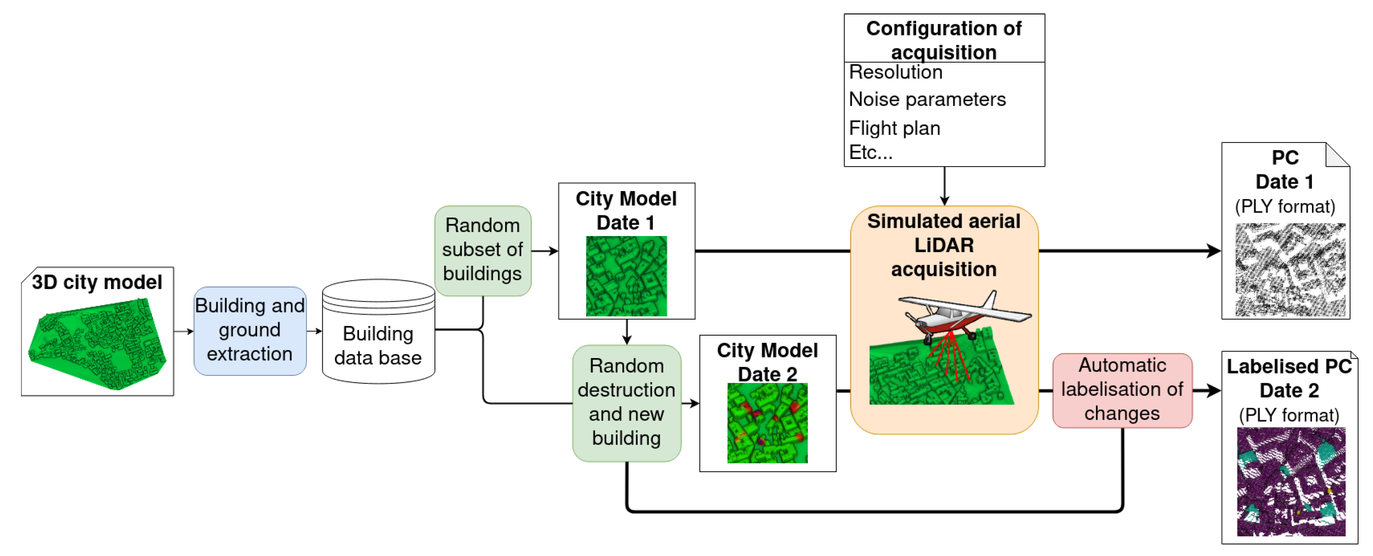
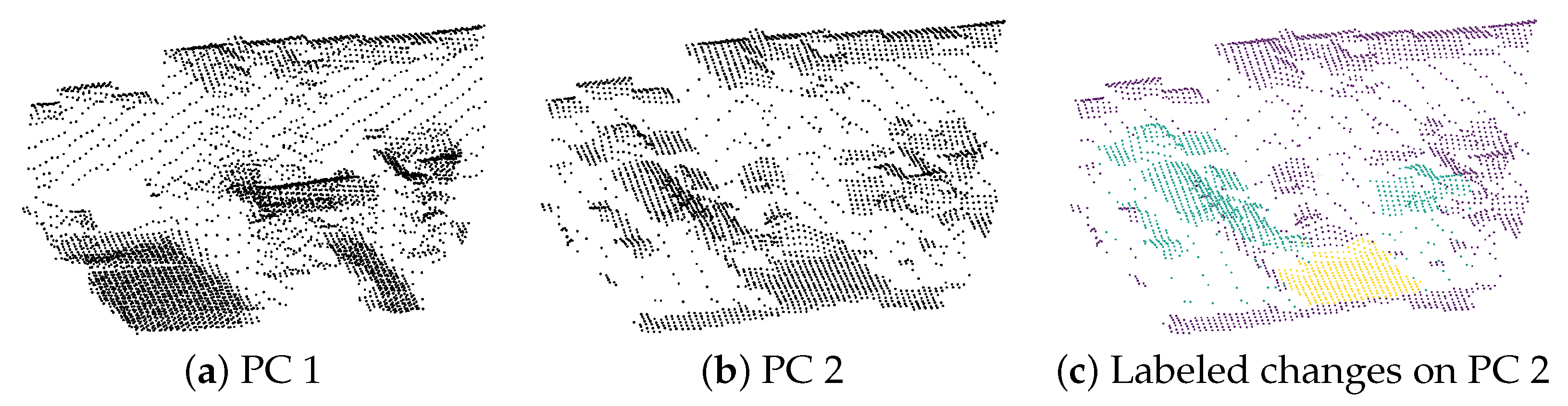
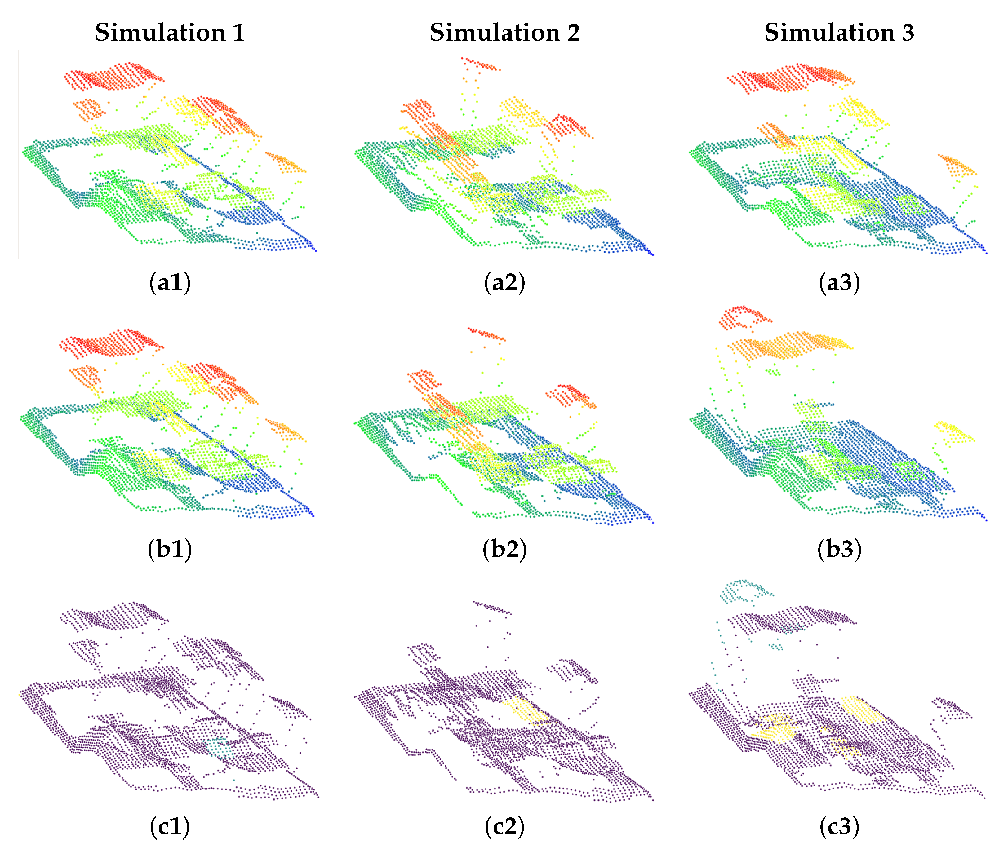
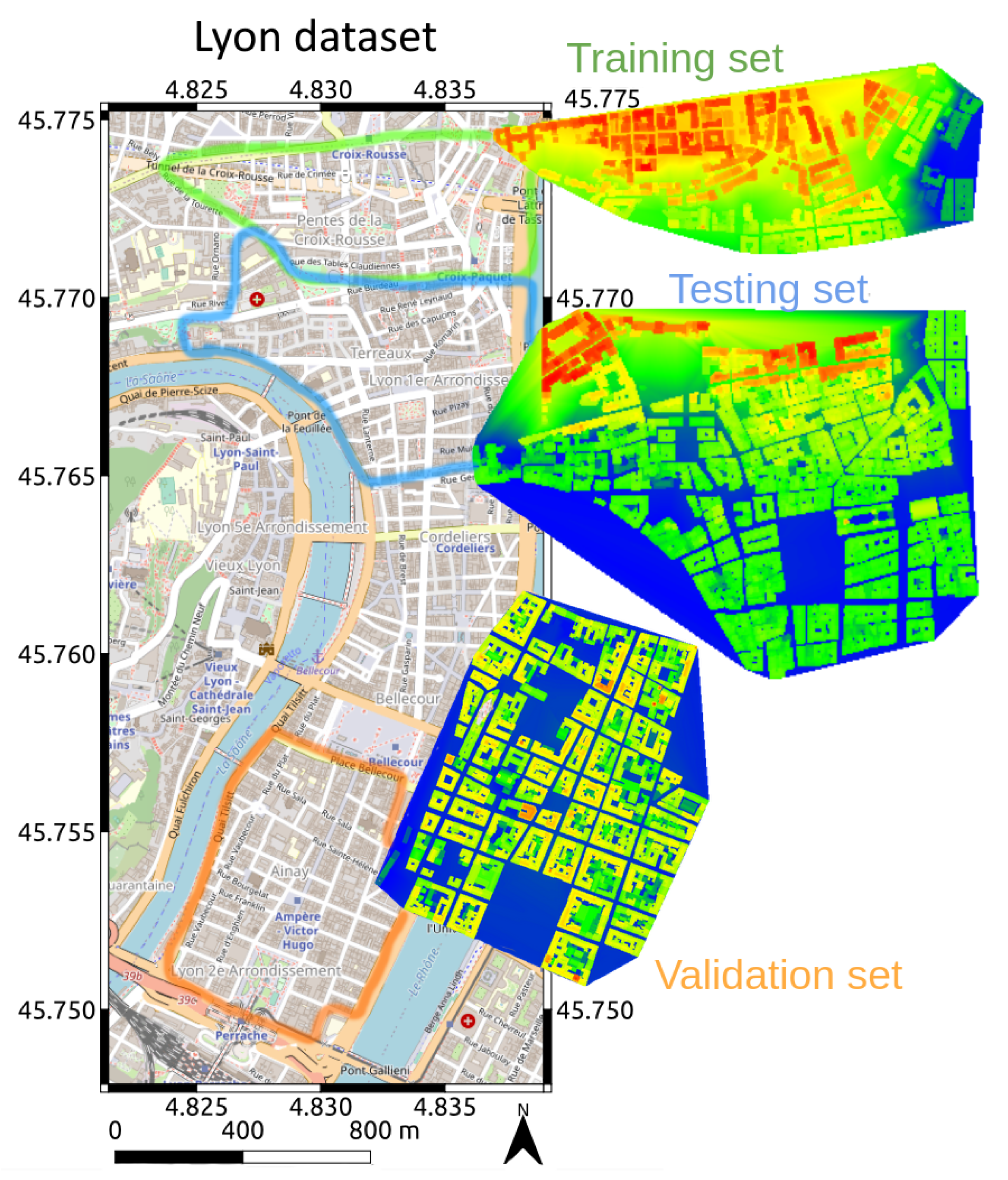
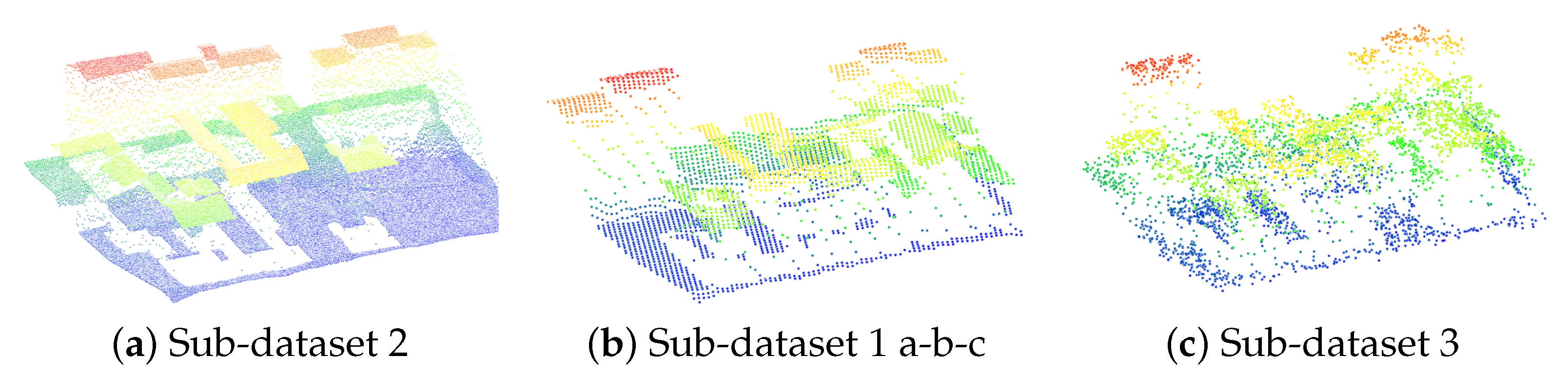
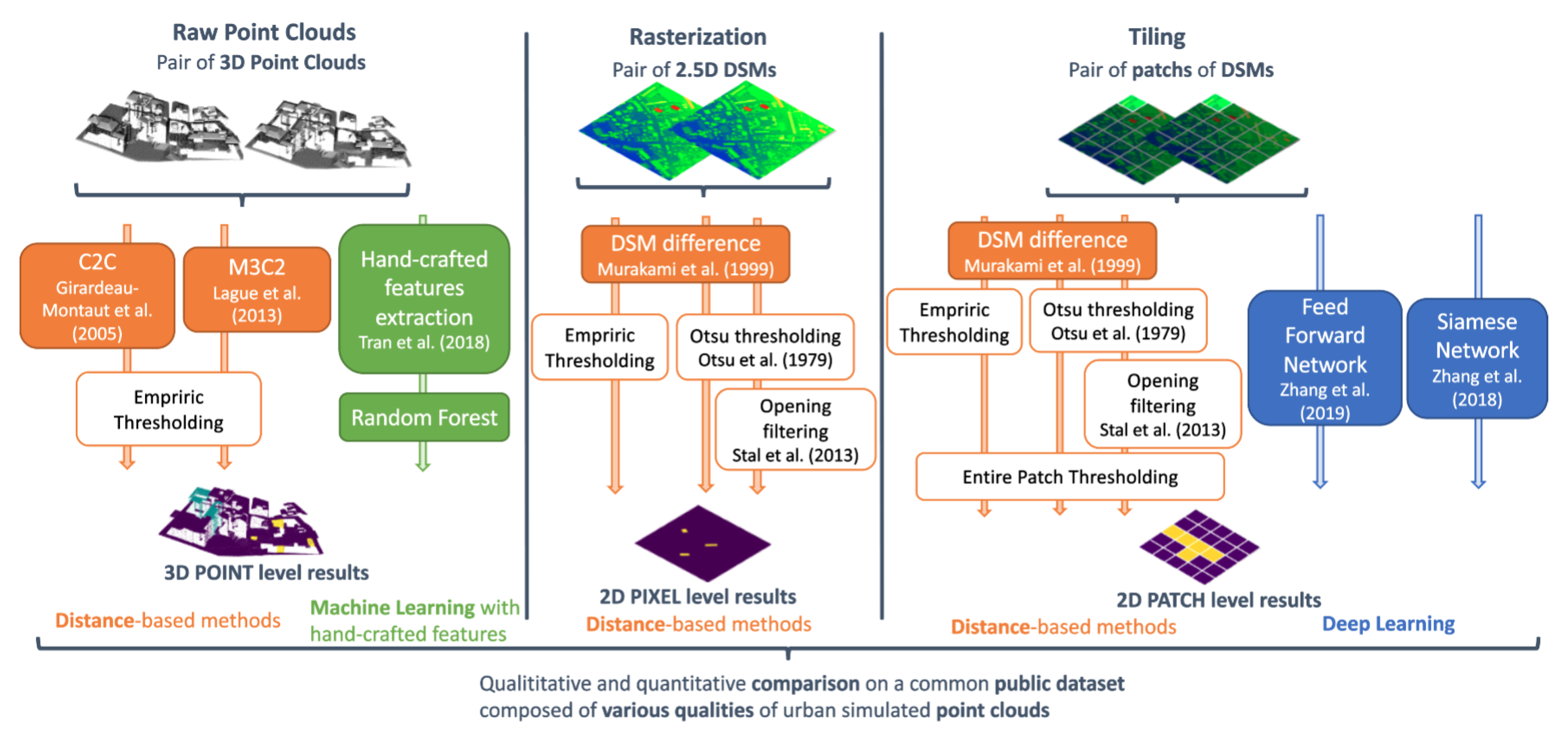
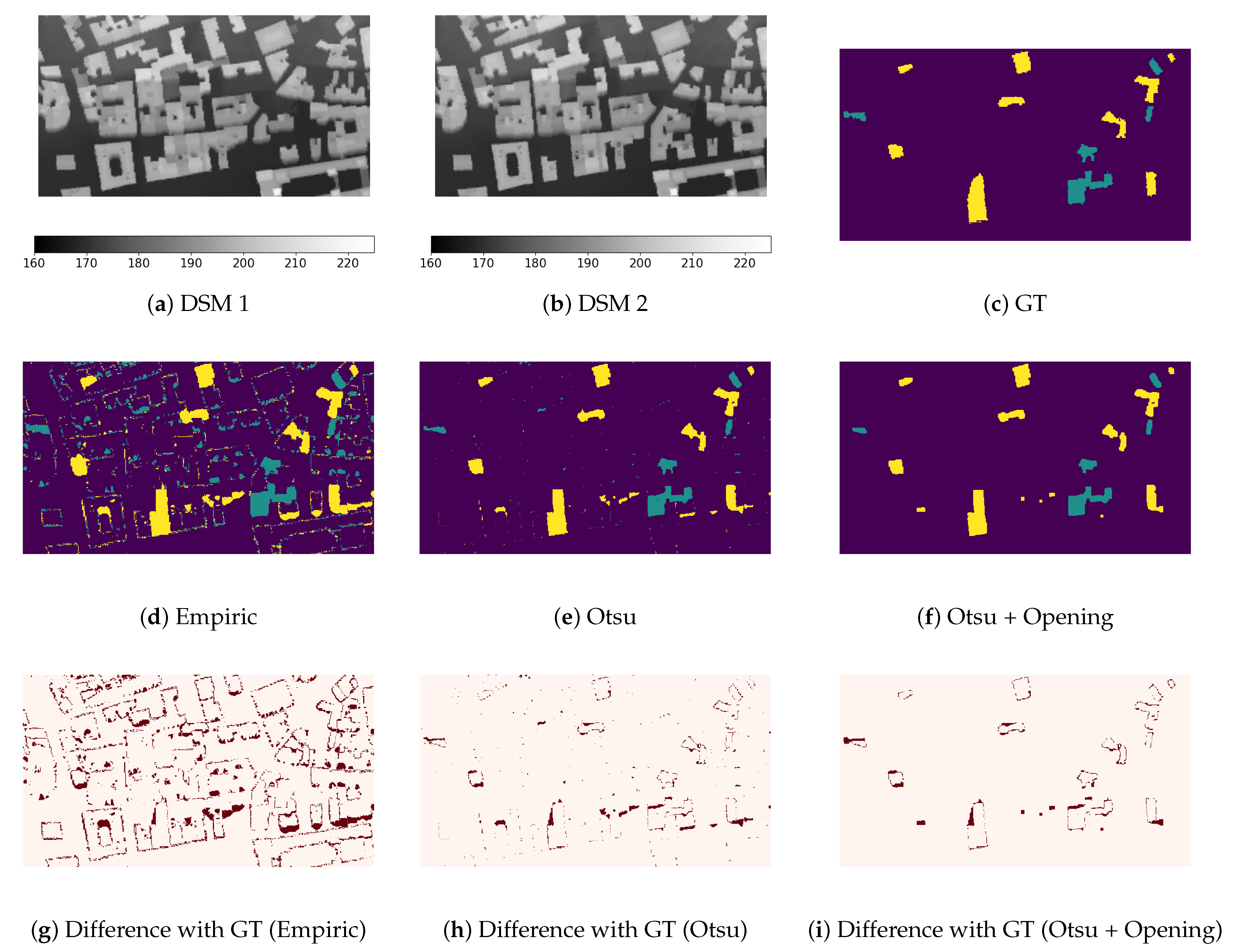
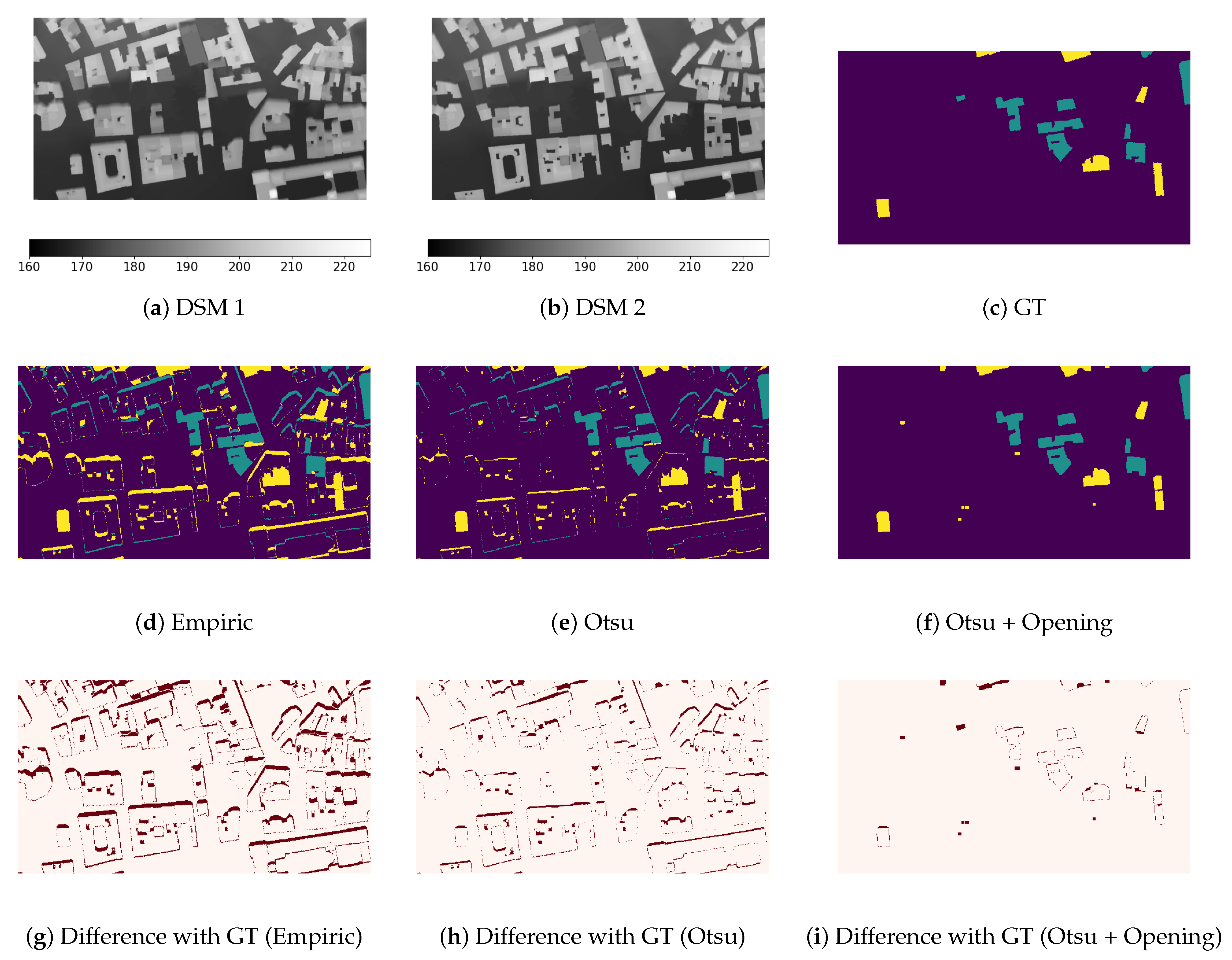
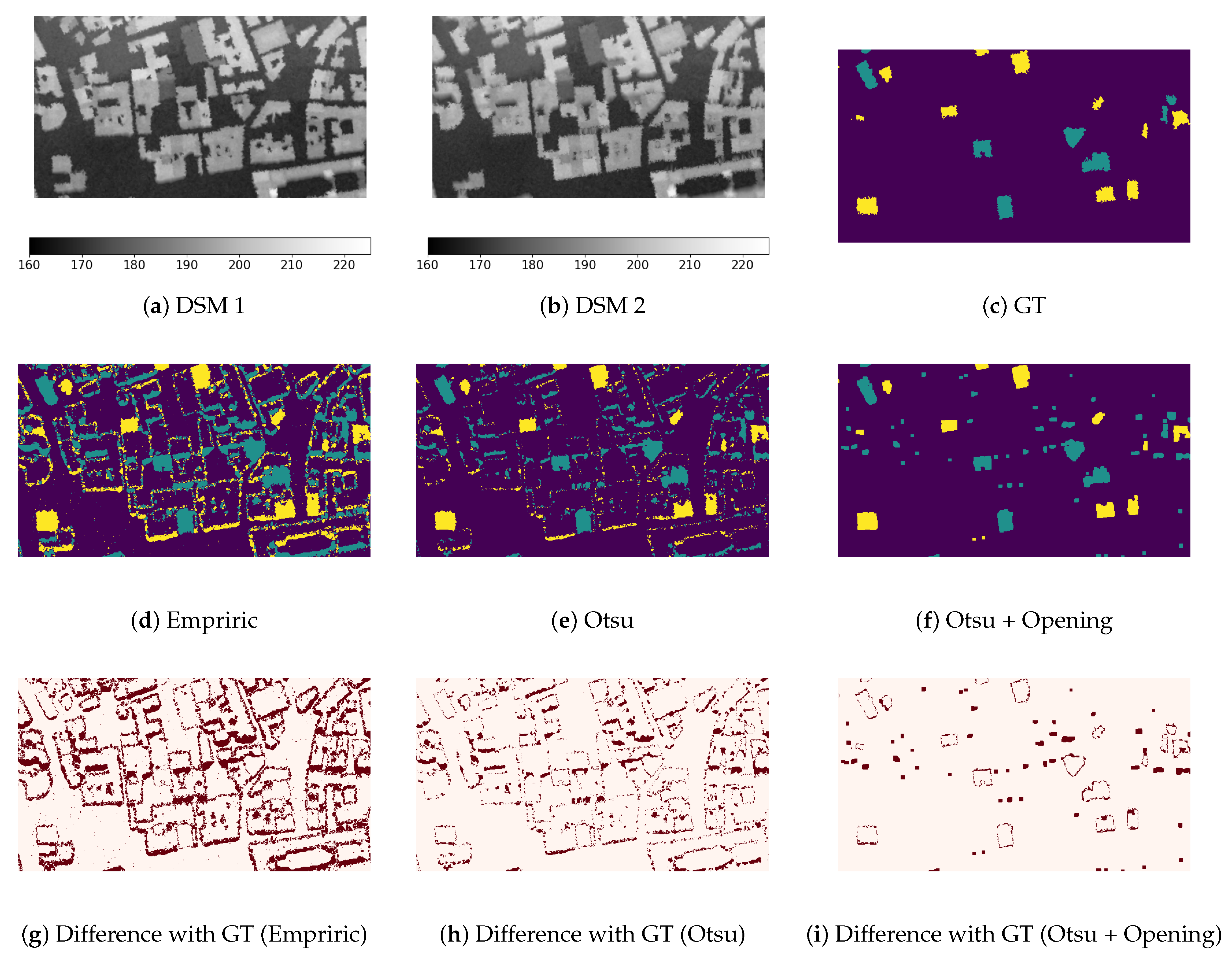
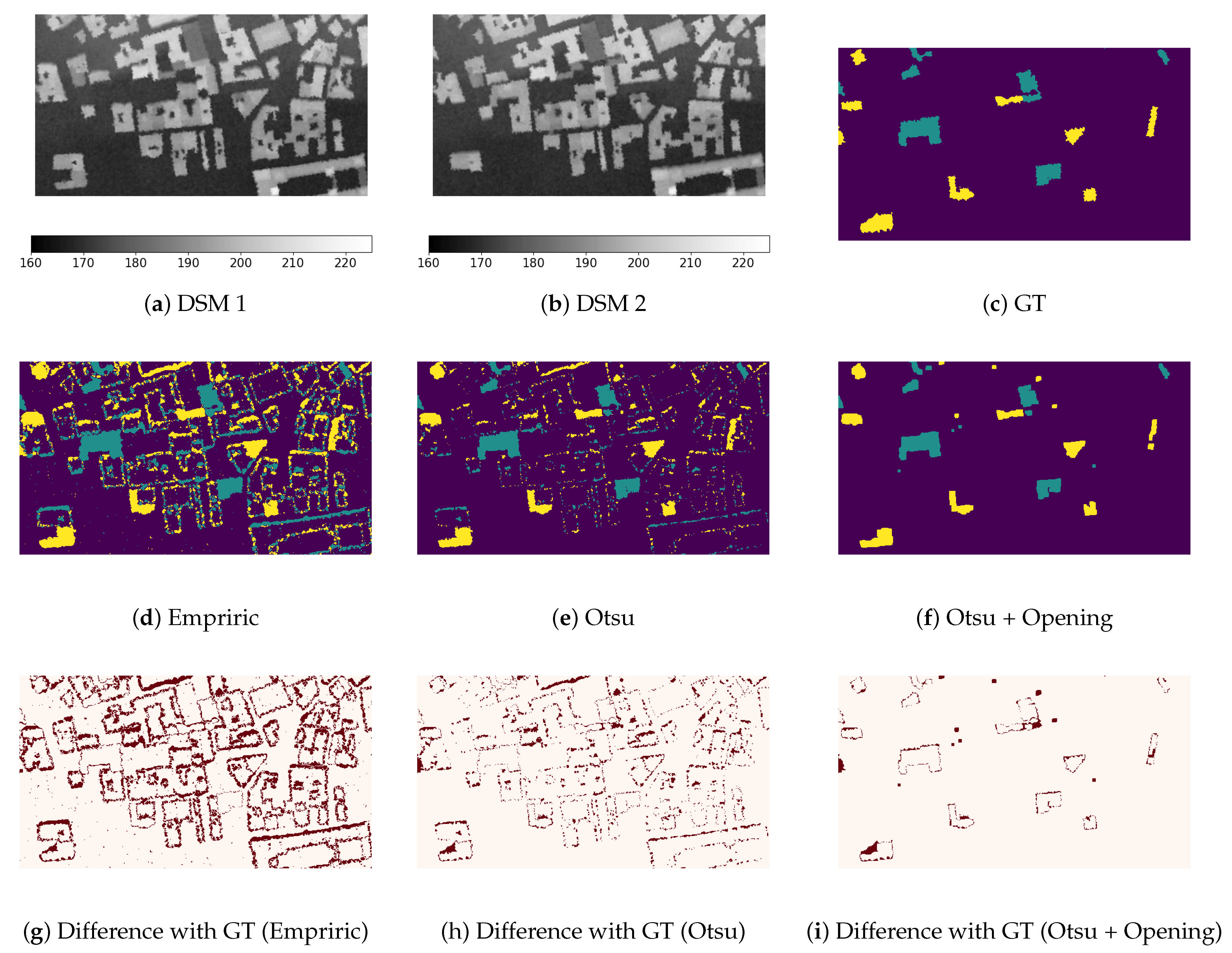
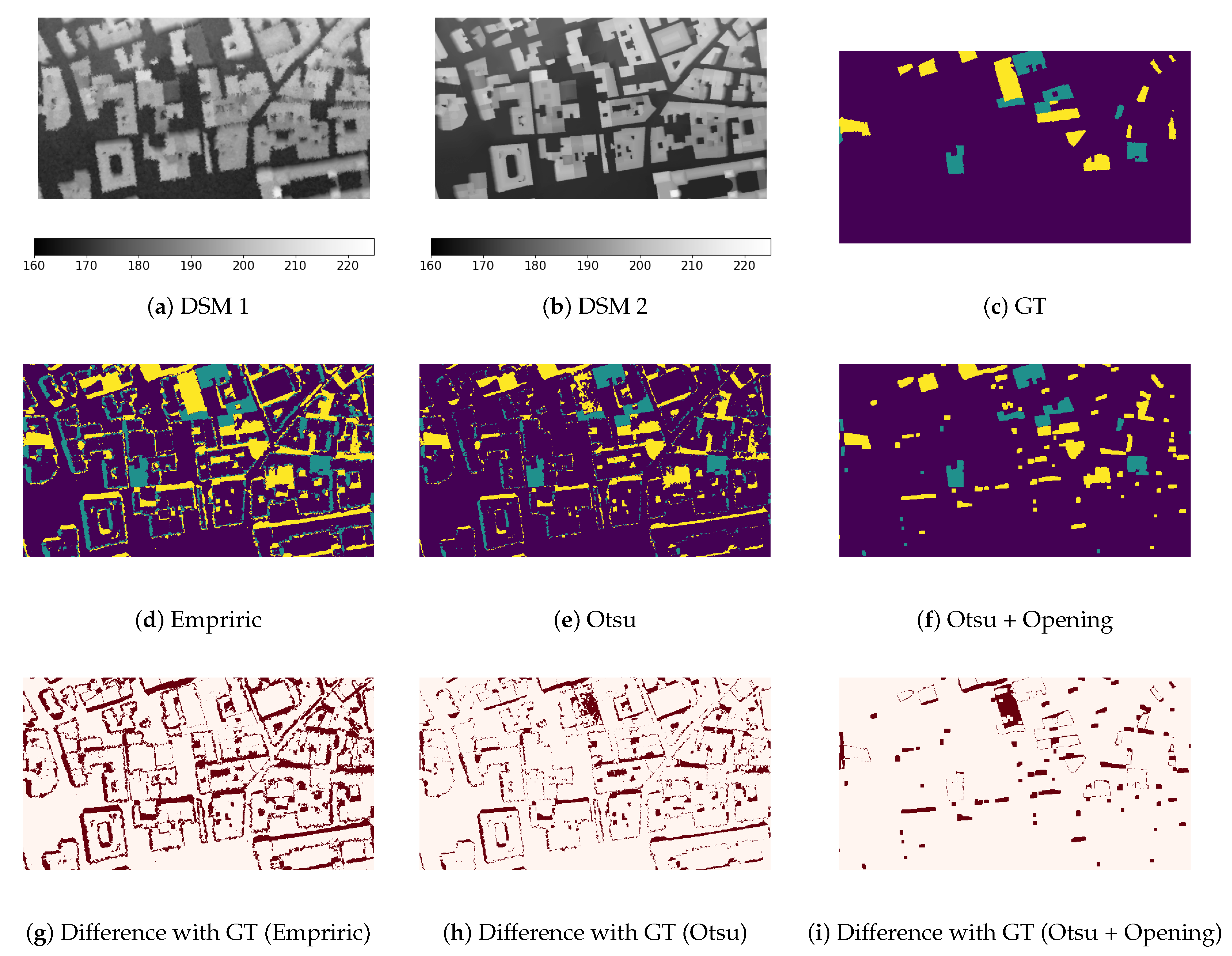
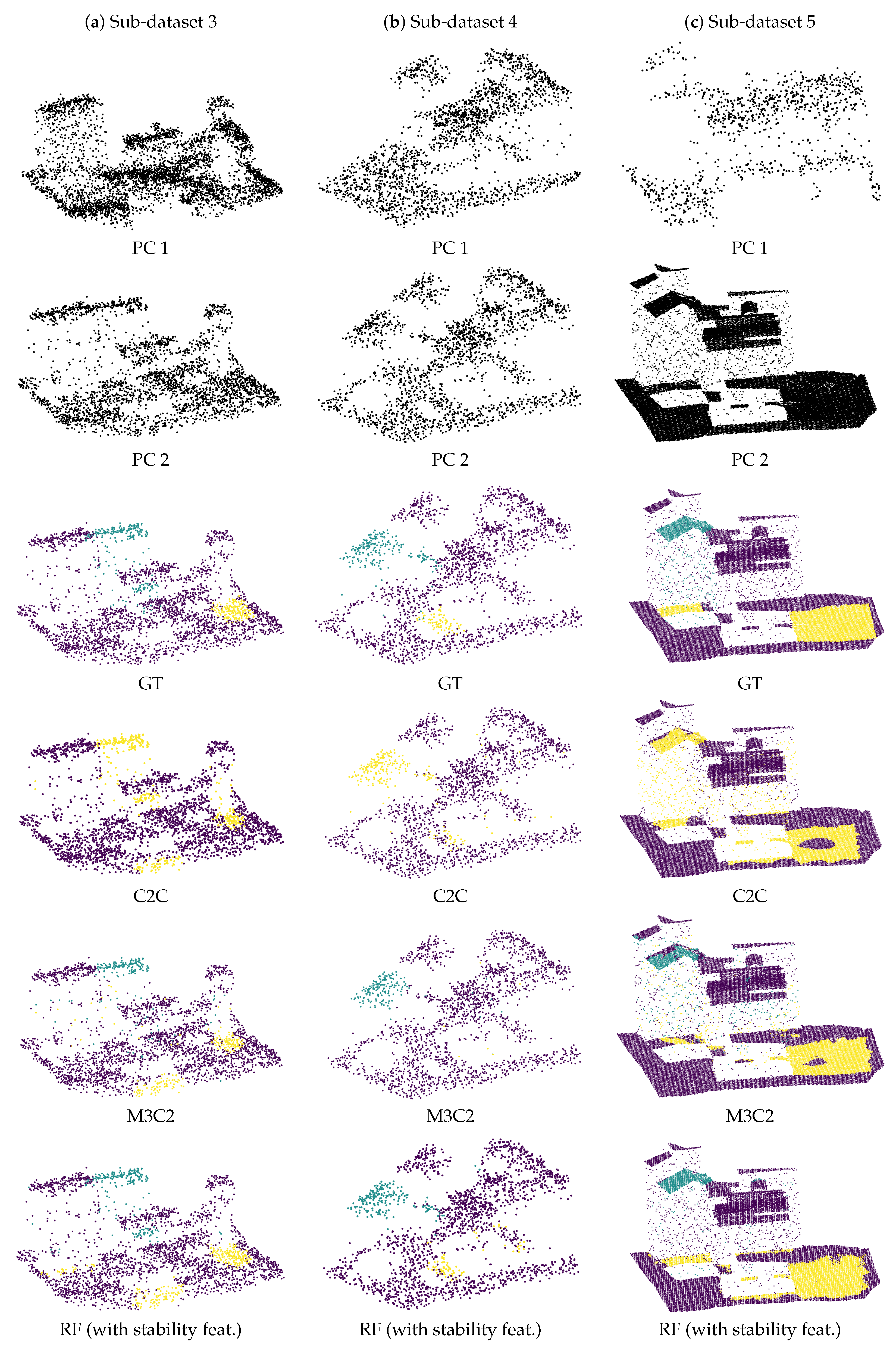
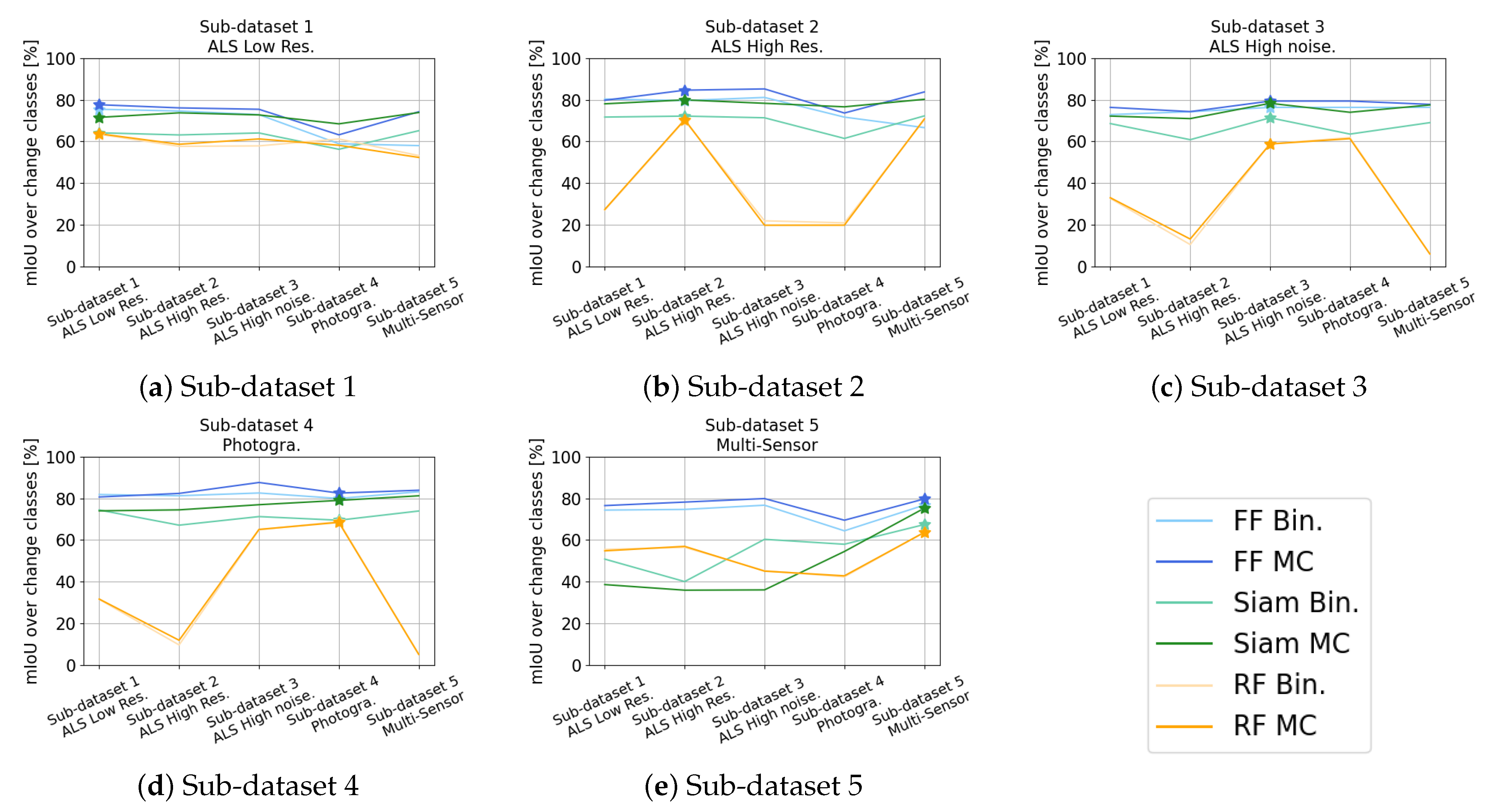
Table 1.
Acquisition configurations for all sub-datasets.
| Sub-Datasets | |||||||
|---|---|---|---|---|---|---|---|
| Parameters | 1 | 2 | 3 | 4 | 5 | ||
| a | b | c | |||||
| Amount of training pairs | 1 | 10 | 50 | 10 | 10 | 10 | 10 |
| Resolution (points/m) | 0.5 | 10 | 0.5 | 0.5 | 0.5/10 | ||
| Noise range across track | 0.01 | 0.01 | 0.2 | 0.2 | 0.2/0.01 | ||
| Noise range along track | 0 | 0 | 0.2 | 0.2 | 0.2/0 | ||
| Noise scan direction (m) | 0.05 | 0.05 | 1 | 1 | 1/0.05 | ||
| Scan angle | 20 to 20 | 20 to 20 | 20 to 20 | −10 to 10 | 20 to 20 | ||
| Overlapping (%) | 10 | 10 | 10 | 5 | 10 | ||
| Height of flight (m) | 700 | 700 | 700 | 700 | 700 | ||
Table 2.
Results of different methods on all sub-datasets at 2D pixel level. Means of IoU over classes of change are given (%). Bin. stands for binary classification results, MC for multi-class classification results, Res. for resolution. For each types of results best values are shown in bold.
Table 2.
Results of different methods on all sub-datasets at 2D pixel level. Means of IoU over classes of change are given (%). Bin. stands for binary classification results, MC for multi-class classification results, Res. for resolution. For each types of results best values are shown in bold.
| Method | Sub-Datasets | ||||||||||
|---|---|---|---|---|---|---|---|---|---|---|---|
| 1 | 2 | 3 | 4 | 5 | |||||||
| ALS Low Res. | ALS High Res. | ALS High Noise | Photogrammetry | Multi-Sensor | |||||||
| Bin. | MC | Bin. | MC | Bin. | MC | Bin. | MC | Bin. | MC | ||
| DSMd + Empiric thresholding | [15] | 37.11 | 36.89 | 50.93 | 50.72 | 30.34 | 29.97 | 30.85 | 30.73 | 33.65 | 33.16 |
| DSMd + Otsu | [15,18] | 59.36 | 59.14 | 67.08 | 66.96 | 53.15 | 52.67 | 54.81 | 54.77 | 53.15 | 52.61 |
| DSMd + Otsu + Opening | [15,18,22] | 72.21 | 71.92 | 79.28 | 79.09 | 70.67 | 70.34 | 76.92 | 76.89 | 71.89 | 70.99 |
Table 3.
Results of different methods on all sub-datasets at the 2D patch level. Means of IoU over classes of change are given (%). Bin. stands for binary classification results, MC for multi-class classification results and Res. for resolution. For each types of results best values are shown in bold.
| Method | Sub-Datasets | ||||||||||
|---|---|---|---|---|---|---|---|---|---|---|---|
| 1 | 2 | 3 | 4 | 5 | |||||||
| ALS Low Res. | ALS High Res. | ALS High Noise | Photogrammetry | Multi-Sensor | |||||||
| Bin. | MC | Bin. | MC | Bin. | MC | Bin. | MC | Bin. | MC | ||
| DSMd + Empiric thresholding | [15] | 36.13 | 34.59 | 50.06 | 48.78 | 30.93 | 29.90 | 31.11 | 30.76 | 32.79 | 31.86 |
| DSMd + Otsu | [15,18] | 62.44 | 60.40 | 76.82 | 75.23 | 58.46 | 56.59 | 72.04 | 71.00 | 56.60 | 55.02 |
| DSMd + Otsu + Opening | [15,18,22] | 82.27 | 80.22 | 88.39 | 86.62 | 83.47 | 80.71 | 88.51 | 86.83 | 82.22 | 79.59 |
| FF Network | [36] | 77.64 | 75.47 | 84.63 | 79.66 | 79.4 | 76.37 | 82.54 | 79.95 | 79.73 | 76.77 |
| Siamese Network | [35] | 71.58 | 64.16 | 79.97 | 72.18 | 78.33 | 71.36 | 79.03 | 69.5 | 75.27 | 67.41 |
Table 4.
Results of different methods on all sub-datasets at the 3D point level. Means of IoU over classes of change are given (%). Bin. stands for binary classification results, MC for multi-class classification results and Res. for resolution. For each types of results best values are shown in bold.
| Method | Sub-Datasets | ||||||||||
|---|---|---|---|---|---|---|---|---|---|---|---|
| 1 | 2 | 3 | 4 | 5 | |||||||
| ALS Low Res. | ALS High Res. | ALS High Noise | Photogrammetry | Multi-Sensor | |||||||
| Bin. | MC | Bin. | MC | Bin. | MC | Bin. | MC | Bin. | MC | ||
| C2C | [37] | 49.59 | - | 61.65 | - | 49.22 | - | 54.75 | - | 49.76 | - |
| M3C2 | [38] | 33.5 | 29.87 | 59.85 | 53.73 | 41.37 | 38.72 | 36.60 | 35.01 | 40.61 | 37.78 |
| RF (with stability feat.) | [46] | 63.70 | 63.41 | 70.48 | 70.12 | 58.78 | 58.83 | 68.46 | 68.87 | 63.65 | 63.64 |
Table 5.
Results of different supervised methods with varying training set sizes (training sets of sub-dataset 1a., 1b. and 1c. contained, respectively, 1, 10 and 50 simulations). Means of IoU over classes of change are given (%). Bin. stands for binary classification results, MC for multi-class classification results, Res. for resolution. For each types of results best values are shown in bold.
| Sub-Datasets | Method at 3D Point Level | Methods at 2D Patch Level | ||||||
|---|---|---|---|---|---|---|---|---|
| RF (with Stability Feat.) [46] | FF [36] | Siamese [35] | ||||||
| Bin. | MC | Bin. | MC | Bin. | MC | |||
| 1 | ALS Low Res. | a | 61.51 | 61.34 | 57.52 | 58.43 | 58.62 | 55.07 |
| b | 63.70 | 63.41 | 77.64 | 75.47 | 71.58 | 64.16 | ||
| c | 67.28 | 67.10 | 81.98 | 77.28 | 78.85 | 66.58 | ||
Publisher’s Note: MDPI stays neutral with regard to jurisdictional claims in published maps and institutional affiliations. |
© 2021 by the authors. Licensee MDPI, Basel, Switzerland. This article is an open access article distributed under the terms and conditions of the Creative Commons Attribution (CC BY) license (https://creativecommons.org/licenses/by/4.0/).
Share and Cite
MDPI and ACS Style
de Gélis, I.; Lefèvre, S.; Corpetti, T. Change Detection in Urban Point Clouds: An Experimental Comparison with Simulated 3D Datasets. Remote Sens. 2021, 13, 2629. https://0-doi-org.brum.beds.ac.uk/10.3390/rs13132629
AMA Style
de Gélis I, Lefèvre S, Corpetti T. Change Detection in Urban Point Clouds: An Experimental Comparison with Simulated 3D Datasets. Remote Sensing. 2021; 13(13):2629. https://0-doi-org.brum.beds.ac.uk/10.3390/rs13132629
Chicago/Turabian Stylede Gélis, Iris, Sébastien Lefèvre, and Thomas Corpetti. 2021. "Change Detection in Urban Point Clouds: An Experimental Comparison with Simulated 3D Datasets" Remote Sensing 13, no. 13: 2629. https://0-doi-org.brum.beds.ac.uk/10.3390/rs13132629
Note that from the first issue of 2016, this journal uses article numbers instead of page numbers. See further details here.