Evaluation and Hydrological Application of a Data Fusing Method of Multi-Source Precipitation Products-A Case Study over Tuojiang River Basin

Abstract

Precipitation is an essential driving factor of hydrological models. Its temporal and spatial resolution and reliability directly affect the accuracy of hydrological modeling. Acquiring accurate areal precipitation needs substantial ground rainfall stations in space. In many basins, ground rainfall stations are sparse and uneven, so real-time satellite precipitation products (SPPs) have become an important supplement to ground-gauged precipitation (GGP). A multi-source precipitation fusion method suitable for the Soil and Water Assessment Tool (SWAT) model has been proposed in this paper. First, the multivariate inverse distance similarity method (MIDSM) was proposed to search for the optimal representative precipitation points of GGP and SPPs in sub-basins. Subsequently, the correlation-coefficient-based weighted average method (CCBWA) was presented and applied to calculate the fused multi-source precipitation product (FMSPP), which combined GGP and multiple satellite precipitation products. The effectiveness of the FMSPP was proven over the Tuojiang River Basin. In the case study, three SPPs were chosen as the satellite precipitation sources, namely the Climate Forecast System Reanalysis (CFSR), Tropical Rainfall Measuring Mission Project (TRMM), and Precipitation Estimation from Remotely Sensed Information using Artificial Neural Network Climate Data Record (PERSIANN-CDR). The evaluation indicators illustrated that FMSPP could capture the occurrence of rainfall events very well, with a maximum Probability of Detection (POD) and Critical Success Index (CSI) of 0.92 and 0.83, respectively. Furthermore, its correlation with GGP, changing in the range of 0.84–0.96, was higher in most sub-basins on the monthly scale than the other three SPPs. These results demonstrated that the performance of FMSPP was the best compared with the original SPPs. Finally, FMSPP was applied in the SWAT model and was found to effectively drive the SWAT model in contrast with a single precipitation source. The FMSPP manifested the highest accuracy in hydrological modeling, with the Coefficient of Determination (R²) of 0.84, Nash Sutcliff (NS) of 0.83, and Percent Bias (PBIAS) of only −1.9%.

1. Introduction

Accurate runoff prediction is conducive to water management and planning, agricultural irrigation [1], climate and human activity impact study [2,3,4], and mitigating the major disasters and losses caused by floods and droughts. At present, the methods of runoff prediction [5,6,7] mainly include two categories: data-driven models and physical models. Data-driven models are comparatively simple to construct, but they cannot explicitly reveal the internal mechanisms of hydrological processes. Physical models, such as semi-distributed hydrological models TOPMODEL [8], variable infiltration capacity [9,10,11], and the Soil and Water Assessment Tool (SWAT) [12] are usually driven by topographic data (e.g., digital elevation model (DEM)), climate data (e.g., precipitation, temperature, and humidity), soil data, and other information at the same time, and their hydrological processes in physical models are more transparent, accurate, and reproducible.

Precipitation is the most important driving factor of physical hydrological models [13]. Its temporal and spatial resolution and reliability directly affect the accuracy of runoff prediction. Generally, the precipitation record mainly comes from traditional meteorological stations, weather radars, and satellite remote sensing [14]. The in-situ precipitation is usually considered to be the most accurate rainfall information source. However, its distribution is very uneven and sparse, especially in some undeveloped areas and mountain ranges, owing to the restriction of economic cost and terrain conditions. In these areas, limited meteorological stations are often used to characterize the areal rainfall of multiple zones with obviously different precipitation patterns. The sparse ground points cannot control the spatial features of rainfall, which may affect accuracy in the hydrological modeling.

The precipitation retrieved by weather radar may carry large system errors due to the block of the electromagnetic beam by the ground. Moreover, its spatial distribution is inconsecutive (the maximum coverage radius of radar is 300 km) [13,15,16]. With the rapid development of satellite remote sensing technology, more and more satellite precipitation products or satellite-based reanalysis precipitation products have been released in recent years (note that all of these satellite precipitation products and reanalysis precipitation products are collectively abbreviated as SPPs in this paper). SPPs can provide broad coverage [17,18] and good spatial continuity. In fact, with the advances of modern remote sensing technology, multiple SPPs have improved their spatial resolution, such as the Climate Forecast System Reanalysis (CFSR), Tropical Rainfall Measuring Mission Project (TRMM), and Precipitation Estimation from Remotely Sensed Information using Artificial Neural Network Climate Data Record (PERSIANN-CDR). The SPPs with high temporal and spatial resolution have become important supplements to in-situ precipitation.

Many studies have been conducted to evaluate the reliability of different SPPs. For example, Liu et al. [19] assessed the streamflow simulation ability of PERSIANN-CDR and Global Land Data Assimilation System precipitation via a hydro-informatic modeling system rainfall-runoff model in the upper Yangtze River basins on the Tibetan Plateau. Their results showed that the streamflow simulated using these two SPPs was consistent with the observations. By contrast, the performance modeled by the sparse in-situ precipitation was not satisfactory in the wet season. Ma et al. [20] evaluated the hydrological simulation reliability of three SPPs via SWAT model over Lancang Basin and found that TRMM fitted best with the observations, followed by PERSIANN-CDR, while CFSR showed unacceptable results. Zhu et al. [21] compared the hydrological performance of SWAT models over two humid basins forced by PERSIANN-CDR, TRMM, and CFSR, respectively, and concluded that the applicability of PERSIANN-CDR and TRMM to streamflow simulation is satisfactory.

Unfortunately, the conclusions about SPPs vary from basin to basin. Which SPP is more suitable for a random study area remains enigmatic. In some basins, the hydrological performance driven by the sparse GGP is sometimes inferior to SPP. Whether SPP is superior to in-situ precipitation is highly dependent on the density of GGP. We are now faced with issues of uncertainty resulting from various precipitation sources, especially over ungauged basins or sparse-data basins. Multi-source precipitation data fusion has thus been a research hotspot in recent years [10]. It can make full use of high-precision ground-gauged precipitation (GGP) and continuously distributed SPPs to form complementary advantages and have broad application prospects [22]. Many fusion methods of multi-source precipitation data have been developed, including the geographically weighted method [13,23,24], machine learning algorithm [25], optimal interpolation method [26], and Bayesian average method [27]. For example, Chao et al. [13] developed eight merging algorithms by combining two geographically weighted regression methods with four weighting functions to get the satellite-gauge precipitation. The new precipitation merged by the CMORPH (CPC MORPHing technique) satellite precipitation and in-situ precipitation performed better than the original CMORPH. Wu et al. [28] proposed a deep fusion method based on the combination of convolutional neural network and long-short-term memory network to merge TRMM and rain gauge data; the method reduced the errors and improved the accuracy of the original TRMM. The basic idea of these fusion algorithms is to establish the correlation between grid precipitation and other geographic variables or climate variables through a linear regression method or non-linear deep learning method to gain the modeled precipitation and then use GGP to correct its deviation and validate the accuracy. Several other studies have used the Bayesian-related method to calculate the respective optimal weights for multiple SPPs and evaluated the simulation capability of the merged precipitation via different hydrological models. For example, Ma et al. [29] developed a merged precipitation dataset combining multiple SPPs based on the Dynamic Bayesian Model Averaging scheme. They evaluated the blended multi-satellite precipitation data in the headwaters of the Yangtze River using the Coupled Routing and Excess Storage model and stated that the merged precipitation showed a promising prospect of hydrological application. Ur Rahman et al. [30] compared the hydrological performance using the SWAT model forced by in-situ precipitation and two merged precipitation products, respectively. The two merged precipitation products produced by multiple SPPs were based on the Dynamic Clustered Bayesian Averaging and Dynamic Bayesian Model Averaging method, respectively, and obtained streamflow forecasting results close to in-situ precipitation.

However, the fusion precipitation on the basis of these methods undergoes multiple processes such as downscaling, resampling, regression, and interpolation, potentially influencing the accuracy of precipitation [25]. Few works investigate fusion precipitation by considering the characteristics of the hydrological model to simplify the fusion processes and hence improve the hydrological applicability of the fused precipitation. This paper proposed a two-step fusion scheme to obtain the fused multi-source precipitation product (FMSPP). First, the multivariate inverse distance similarity method (MIDSM) has been proposed and applied to search for the optimal representative precipitation points of GGP and SPPs. Second, the correlation-coefficient-based weighted average (CCBWA) method was presented and employed to construct the FMSPP based on multiple SPPs and GGP. In this study, the satellite precipitation sources included CFSR, TRMM, and PERSIANN-CDR. The effectiveness of the fusion method was proven through two aspects. First, the accuracy of FMSPP was evaluated by comparison with the distribution of original SPPs on different temporal and spatial scales. Secondly, FMSPP, GGP, and every SPP were used to drive the SWAT model. The corresponding simulated streamflow was compared with the observations to evaluate their applicability in the hydrological model.

The rest of this paper is organized as follows. Section 2 describes the study basin and data preparation. Section 3 presents the methodology. The results and discussion are given in Section 4 and Section 5, respectively. Finally, Section 6 summarizes the study.

2. Study Basin and Data Preparation

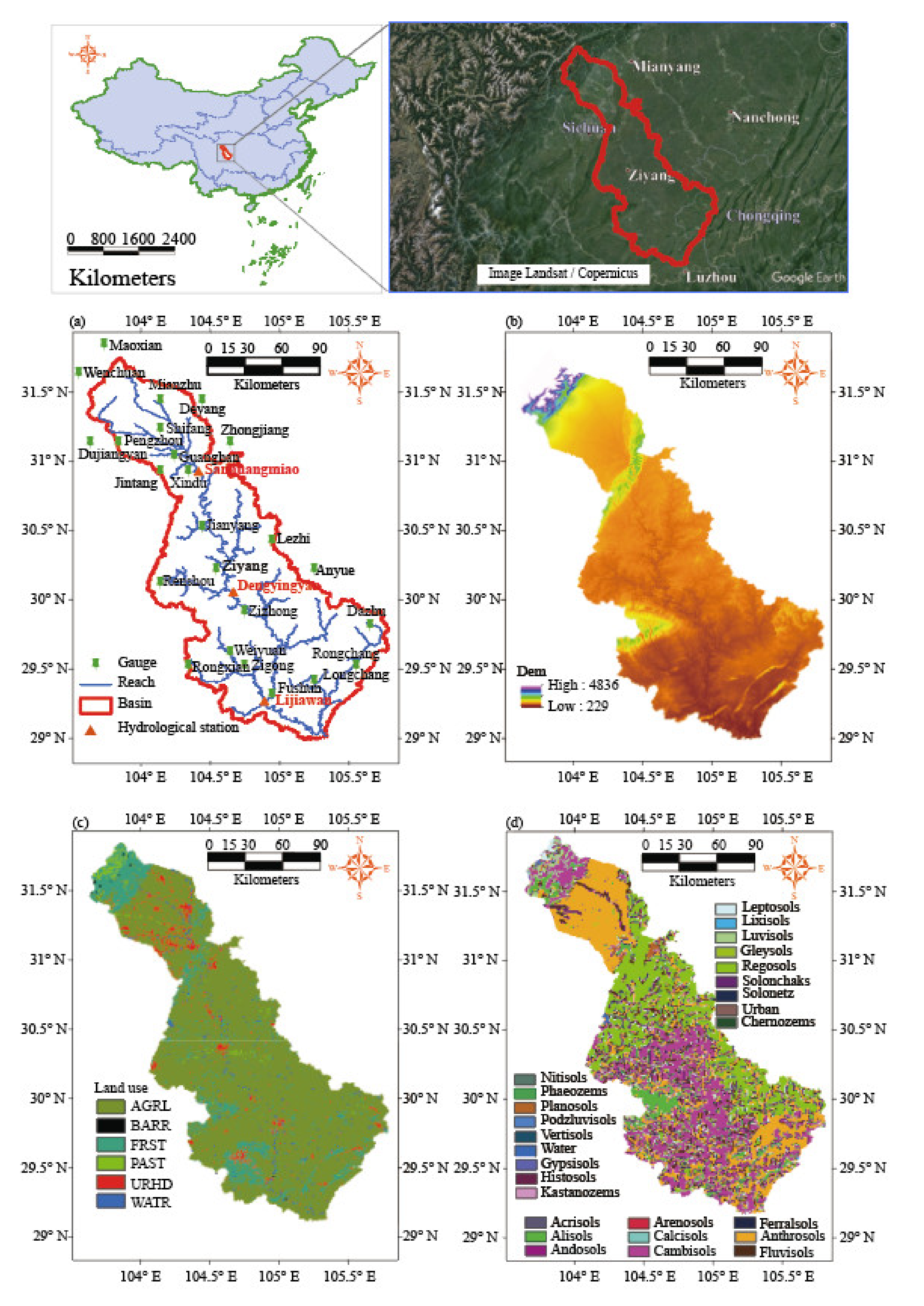
2.1. Study Basin

The Tuojiang River is a major tributary of the upper reaches of the Yangtze River, with a length of 502 km and a total basin area of 27,860 km², spanning between 103°38′ and 105°50′ East and 27°50′ to 31°41′ North. Figure 1 shows the geographic locations of the Tuojiang River Basin (TJRB). Twenty-four ground meteorological stations were distributed within or near the TJRB (

Table 1. The geographic information of the ground meteorological stations and the gauged average annual precipitation.

Name	Latitude (°N)	Longitude (°E)	Elevation (m)	Annual Precipitation (mm)
Maoxian	31.7	103.8	1590.1	633.5
Wenchuan	31.5	103.6	1370.1	632.0
Mianzhu	31.3	104.2	589.0	1181.7
Dujiangyan	31.0	103.7	698.5	1351.2
Pengzhou	31.0	103.9	581.7	1017.9
Shifang	31.1	104.2	535.7	1049.3
Deyang	31.3	104.5	525.7	966.2
Zhongjiang	31.0	104.7	423.5	985.0
Xindu	30.8	104.2	514.5	966.0
Guanghan	30.9	104.3	469.0	913.7
Jianyang	30.4	104.5	448.5	939.7
Jintang	30.8	104.4	493.5	957.0
Renshou	30.0	104.2	436.5	1070.5
Ziyang	30.1	104.6	417.0	1025.2
Zizhong	29.8	104.8	369.4	1161.6
Rongxian	29.4	104.4	384.1	1126.1
Weiyuan	29.5	104.7	351.1	1083.2
Zigong	29.4	104.8	352.6	1162.3
Fushun	29.2	105.0	306.2	1150.4
Lezhi	30.3	105.5	462.6	1108.5
Anyue	30.1	105.3	383.6	1182.3
Dazu	29.7	105.7	394.7	1178.4
Rongchang	29.4	105.6	338.0	1220.5
Longchang	29.3	105.3	385.7	1180.2

and Figure 1a). The TJRB is located in the subtropical humid monsoon climate zone, with the characteristics of a mild climate, abundant rainfall, and four distinct seasons. It traverses the mountainous areas on the western edge of Sichuan, Chengdu Plain, and hilly regions of the central Sichuan Basin. The climate between the north and the south differs due to the complex terrain and the elevational difference. The temperature gradually rises from the northwest to the southeast. The annual mean temperature in mountainous areas is 15.7 °C and in hilly areas its 17.6 °C. Rainfall is heavier in the mountains compared to the hills. For example, the annual mean precipitation is 1200–1500 mm in the Lutou Mountain rainstorm area, 1000–1400 mm in the Chengdu Plain, and only 900 mm in the hilly area. Precipitation is more concentrated in the summer, accounting for about 60% of the total annual precipitation, while winter only accounts for 4%.

2.2. Precipitation Data and Other Data

In this study, the in-situ precipitation data measured by the 24 ground meteorological stations were acquired from the China Meteorological Data Service Center. Other meteorological data required for the SWAT model, such as temperature, humidity, and wind speed, were also collected from ground measurements. Three types of SPPs with daily scale and spatial resolution of 0.25° were selected, namely, CFSR, TRMM-3B42, and PERSIANN-CDR. The brief information about the aforementioned four precipitation products is shown in

Table 2. Satellite and in-situ precipitation products used in this watershed.

Dataset	Data Type	Spatial Resolution	Time Resolution	Period	Data Source
CFSR	Reanalysis	0.25 × 0.25	Daily	1979–2014	https://globalweather.tamu.edu/ (accessed on 3 July 2021)
TRMM	Satellite	0.25 × 0.25	Daily	1998–2019	https://disc.gsfc.nasa.gov/datasets?keywords=TMPA&page=1 (accessed on 3 July 2021)
PERSIANN-CDR	Satellite	0.33 × 0.33	Daily	1983–2019	https://chrsdata.eng.uci.edu/ (accessed on 3 July 2021)
GGP	in-situ measurement	24 stations	Daily	1978–2019	http://data.cma.cn/ (accessed on 3 July 2021)

. Figure 2 displays the spatial distribution of different precipitation products. For a more detailed introduction to SPPs, please refer to the literature [21,31]. The monthly streamflow spanning from 1980–2008 measured at the three hydrological stations, namely Sanhuangmiao, Dengyinyang, and Lijiawan, was collected. These three hydrological stations, shown in

Table 3. Hydrological stations over TJRB and their measured average annual streamflow.

Hydrometric Station	Drainage Area (km2)	Annual Average Streamflow (m3/s)
Sanhuangmiao	6590	230.9
Dengyinyan	14,484	286.7
Lijiawan	23,283	397.8

and Figure 1a, are located at the upper, middle, and downstream areas of the TJRB, respectively.

The Harmonized World Soil Database provided by the Food and Agriculture Organization of the United Nations is used for the soil data and reclassified into 27 types with a spatial resolution of 1 km (Figure 1d). The land use (Figure 1c) is obtained from the Resource and Environmental Science and Data Center (RESDC) and divided into six categories with a spatial resolution of 1 km, of which agricultural land accounts for 80.75%, and forest land accounts for 12.4%. DEM comes from Shuttle Radar Topography Mission, with a spatial resolution of 90 m (Figure 1b and

Table 4. Topographic data required for SWAT model and other related data used in the methodology.

Data Type	Spatial Resolution	Period	Data Source
Soil	1 km	1997	http://www.fao.org/soils-portal/en/ (accessed on 3 July 2021)
Land Use	1 km	2005	http://www.resdc.cn/Default.aspx (accessed on 3 July 2021)
DEM	90 m	2000	https://portal.opentopography.org/datasets (accessed on 3 July 2021)
NDVI	1 km	1998–2008	http://www.resdc.cn/Default.aspx (accessed on 3 July 2021)

). The elevation of the basin is approximately 4800 m in the northwest while as low as 250 m in the southeast. As for the catchment shape, the upper part is narrow, and the lower part is wide. The Tuojiang River flows into the Yangtze River in southern Luzhou City. The standardized difference vegetation index (NDVI) from 1998 to 2008 provided by the RESDC is adopted for MIDSM, with a spatial resolution of 1 km.

3. Methodology

3.1. SWAT Model

SWAT is a physically-based semi-distributed hydrological model developed by the Agricultural Research Service of the United States Department of Agriculture [32]. The smallest calculation unit is the HRU, which is grouped by the fields of soil, land use, and slope together to simplify a run. About 1–10 HRUs gather into a sub-basin, and the flow generated and converged in each sub-basin flows into the connected river. A sub-basin is used to represent the precipitation of all internal homogeneous HRUs and distinguish the precipitation source. SWAT simulates the water cycle process according to the water balance equations:

$$S{W}_t=S{W}_0+{\displaystyle \sum _{i=1}^t(PREC-SURQ-ET-WSEEP-GWQ)}$$

(1)

$$WYLD=SURQ+GWQ+LATQ-TLOSS$$

(2)

where SW₀ and SW_t are the initial and final water contents in the soil, respectively; PREC represents the precipitation; SURQ denotes the surface runoff; ET is the evapotranspiration; WSEEP means the amount of water that percolates or bypasses from the bottom of the soil profile; GWQ and LATQ are groundwater flow and lateral flow generated from each HRU, respectively; TLOSS is the amount of water lost from the reach through bed transmission; WYLD represents the net water contributed by the HRU to the reach.

In the SWAT model, climate data is read in the format of point records. The nearest station is selected as the precipitation source of the sub-basin based on the principle of the smallest distance from the geometric center of each sub-basin to the rainfall point. Each sub-basin can only be represented by the nearest precipitation point to characterize the spatial distribution of the entire sub-basin. The area of sub-basins should not be too small; otherwise, the hydrological calculations are immense.

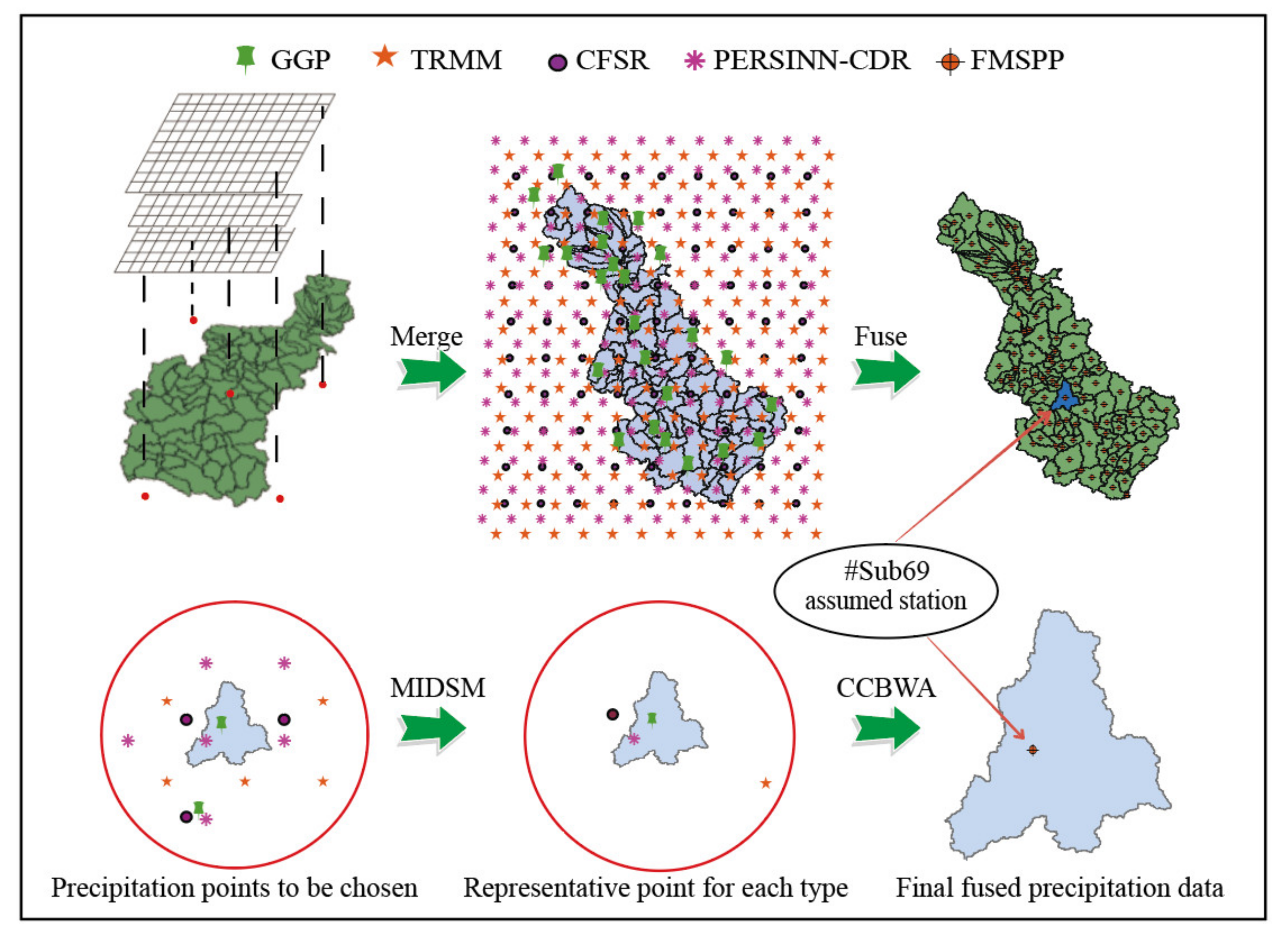
3.2. The Multi-Source Precipitation Fusing Method

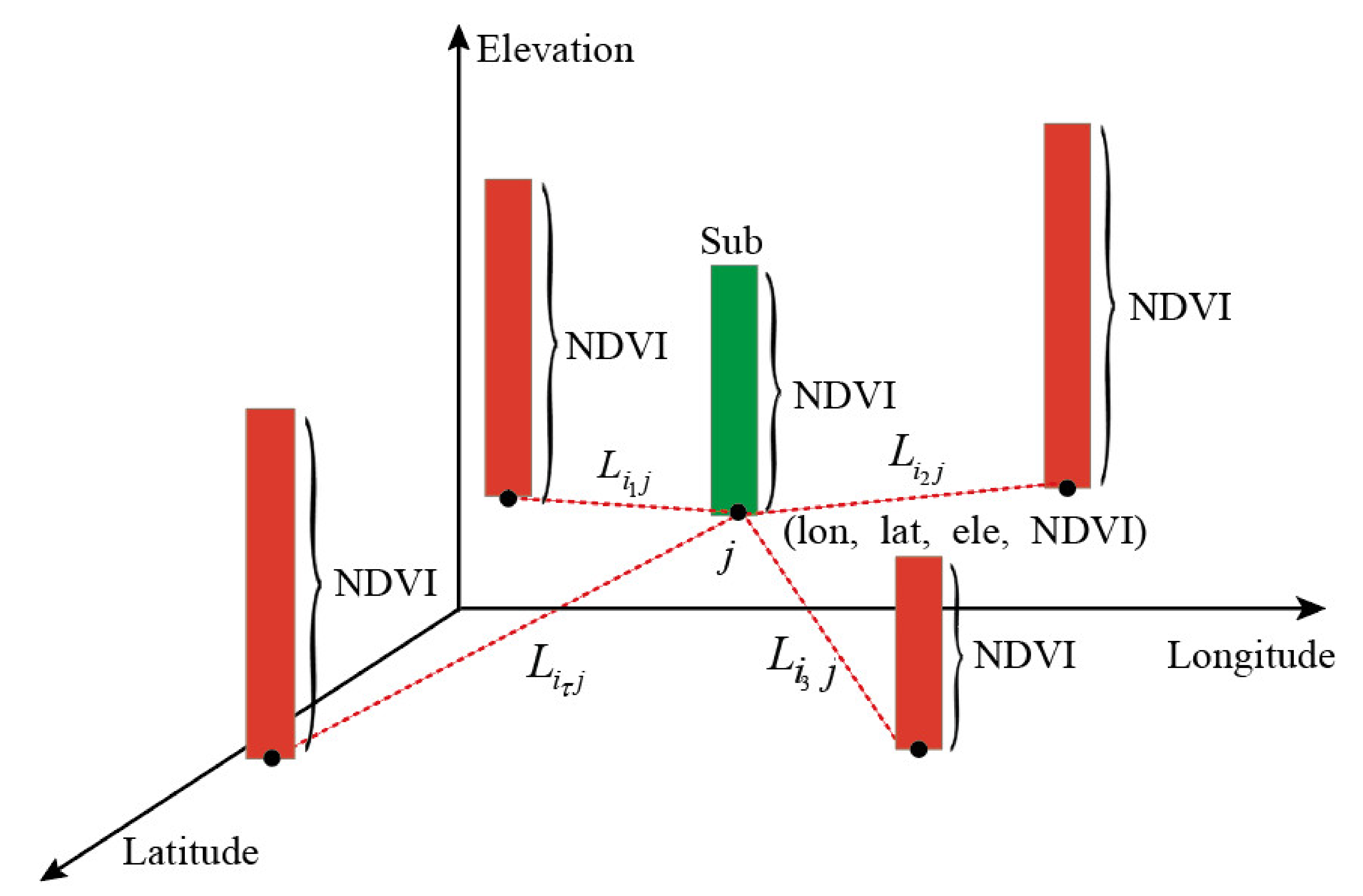
A two-step fusion method has been proposed. First, the multivariate inverse distance similarity method (MIDSM) is proposed to search for the optimal representative precipitation points of the GGP and SPPs. Second, the correlation-coefficient-based weighted average (CCBWA) method is presented and applied to form the fused multi-source precipitation product (FMSPP). FMSPP is the weighted average of the GGP and multiple satellite precipitation products. Multiple SPPs and the GGP compose an open database, and the SPPs involved in the database are not restricted to any particular type. All reliable satellite precipitation products developed in the future can participate, and unreliable satellite data can be eliminated. In the case study of this paper, three mainstream SPPs are chosen as the satellite precipitation sources, namely CFSR, TRMM, and PERSIANN-CDR. Unlike previous satellite-gauge fusion methods to establish a new grid precipitation field, the proposed method focuses on the real precipitation point chosen by the SWAT model. Moreover, the method aims to establish the sub-basin precipitation field and create assumed weather stations located at the geometric centers of sub-basins, facilitating SWAT to select these weather stations as the precipitation source automatically. Figure 3 illustrates the two-step fusing process of FMSPP. The fused precipitation is mathematically expressed as:

$$P_j^{fuse}={\displaystyle \sum _{i_{\tau }=i_1}^m{P}_j^{i_{\tau }}\times }\hspace{0.33em}{W}_j^{i_{\tau }}$$

(3)

where P_j^fuse is the fused precipitation for the sub-basin j; $P_j^{i_{\tau }}$ is the precipitation at the representative precipitation point for product i_τ, in sub-basin j; $W_j^{i_{\tau }}$ is the weight of the precipitation product i_τ, in sub-basin j.

Note that this is a dynamic fusing process. $W_j^{i_{\tau }}$ is not a fixed value, and it is varying in the sub-basins. Furthermore, the database can be updated, and FMSPP dynamically fuses all available in-situ and satellite datasets over the time span (Figure 4).

3.2.1. MIDSM

How to choose the representative precipitation point for the sub-basin? Multivariate inverse distance similarity method (MIDSM) is proposed. MIDSM is based on inverse distance weighting (IDW). IDW [33], also known as the reciprocal distance multiplication method, is a geographic interpolation method based on the principle of similarity. Each data point has a certain influence on the interpolation point. The smaller the distance between the estimated and measured points, the greater the weight, and vice versa.

Precipitation is not only influenced by spatial location but also significantly correlates with elevation and NDVI [34]. Vegetation coverage in the continental area of China reflects the distribution of annual precipitation. The positive relationship between precipitation and NDVI was indicated in the Refs. [35,36]. A quantitative analysis about how NDVI responds to precipitation was made in Yellow-Huai-Hai River Basin [37], and it was concluded that 10% of increased precipitation would obtain 3.35–4.80% increase in NDVI. These findings indicate that increased precipitation is critical for the growth of most of the vegetation types. Herein, we take these four variables into consideration and propose the MIDSM to optimize selecting precipitation points for sub-basins. The precipitation point with the smallest generalized distance or the most significant similarity between the precipitation data points and the geometric center is selected as the precipitation source for the sub-basin. Figure 5 shows a schematic of the MIDSM, and the specific steps to apply this method are as follows.

(1) All grid centers of SPPs are extracted as the rainfall points (Figure 2). SPPs and GGP are distributed within or around each sub-basin, which significantly improves the alternatives of rainfall points.

(2) The watershed is delineated into 116 sub-basins by the SWAT model. Attributes including longitude, latitude, elevation, and NDVI are assigned to the precipitation data points and the geometric center of sub-basins. The generalized distance and the similarity between the geometric center point and the rainfall point can be calculated with Equations (4) and (5):

$$L_{i_{\tau }kj}=\sqrt{{(lo{n}_j-lo{n}_{i_{\tau }k})}^2+{(la{t}_j-la{t}_{i_{\tau }k})}^2+{(el{e}_j-el{e}_{i_{\tau }k})}^2+{(NDV{I}_j-NDV{I}_{i_{\tau }k})}^2} k=1,2,\cdots ,n$$

(4)

$$S_{i_{\tau }kj}=\frac{\frac{1}{L_{i_{\tau }kj}}}{{\displaystyle \sum _{k=1}^n\left(\frac{1}{L_{i_{\tau }kj}}\right)}}$$

(5)

where i_τ (= i₁, i₂,…, i_m) represents the precipitation products (GGP, CFSR, TRMM, and PERSIANN-CDR for the case study in this paper); j is the sub-basin number, and j ∈ [1, 116]; lon, lat, ele, and NDVI are the longitude, latitude, elevation, and NDVI, respectively, and the four variables have been normalized. $L_{i_{\tau }kj}$ and $S_{i_{\tau }kj}$ denote the generalized distance and the similarity between the k (= 1,2,...,n) rainfall point of precipitation product i_τ and the center point of sub-basin j, n is the number of grid centers of SPPs or observed stations of GGP in the search area.

The rainfall data point with the most significant similarity (the smallest generalized distance) is selected as the optimal representative point for each precipitation product, its precipitation is $P_j^{i_{\tau }}$.

3.2.2. CCBWA

How to calculate the $W_j^{i_{\tau }}$ for product i_τ? The correlation coefficient-based weighted average (CCBWA) method has been suggested. CCBWA integrates multiple rainfall points screened by MIDSM into FMSPP and establishes the corresponding assumed station point located in the geometric center. Because the monthly-scale precipitation is more consistent and less biased than the daily-scale precipitation [38,39], the monthly scale CC has been chosen to calculate the weighting factors. The weighting factor is mathematically expressed as:

$$W_j^{i_{\tau }}=\frac{C{C}_j^{i_{\tau }}}{{\displaystyle \sum _{\tau =1}^{m}C{C}_j^{i_{\tau }}}}\tau =1,2,\cdots ,m$$

(6)

where $C{C}_j^{i_{\tau }}$ is the correlation coefficient of precipitation product i_τ, in sub-basin j, against GGP; m is the number of precipitation products, here m = 4.

4. Result

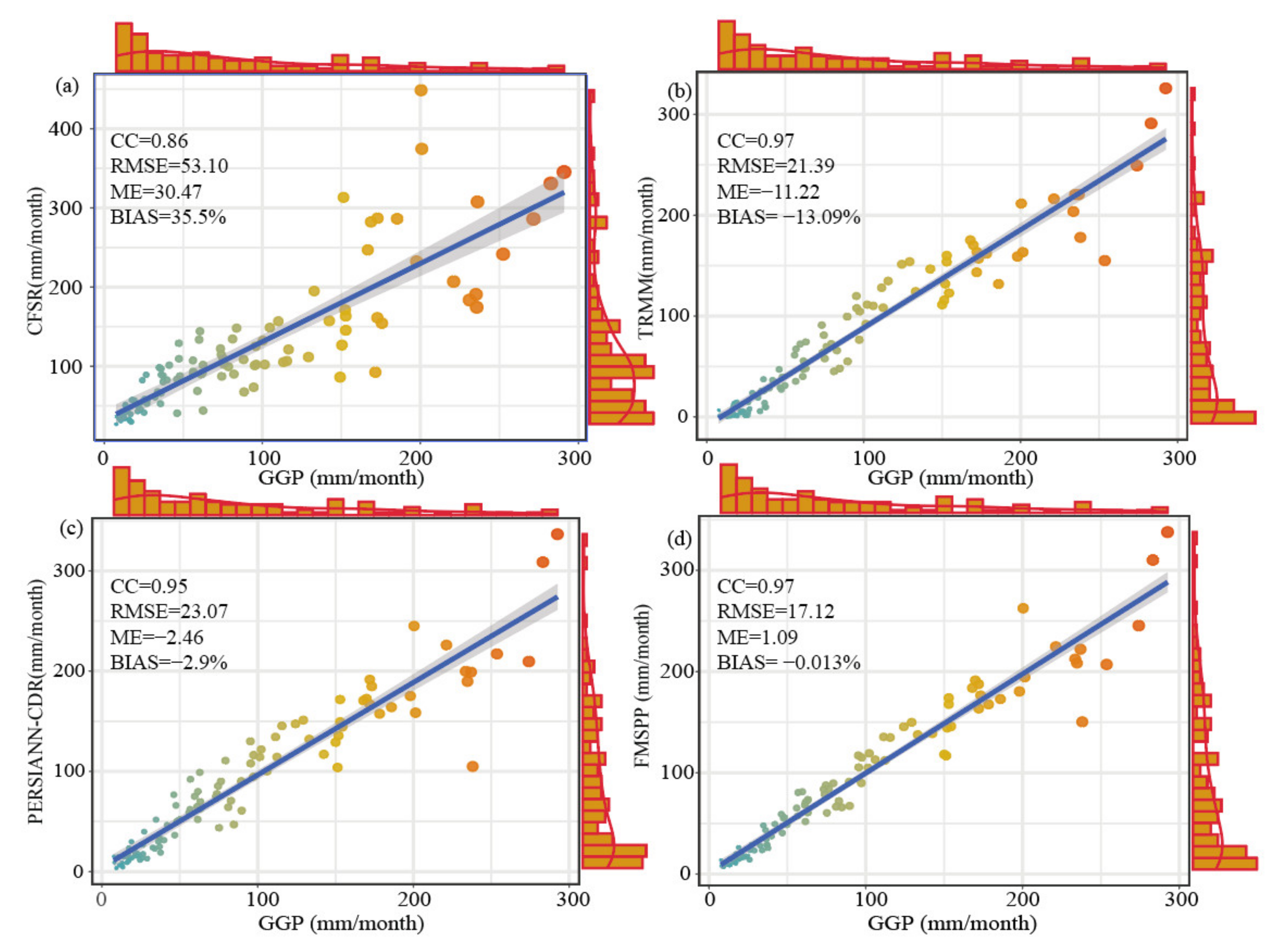
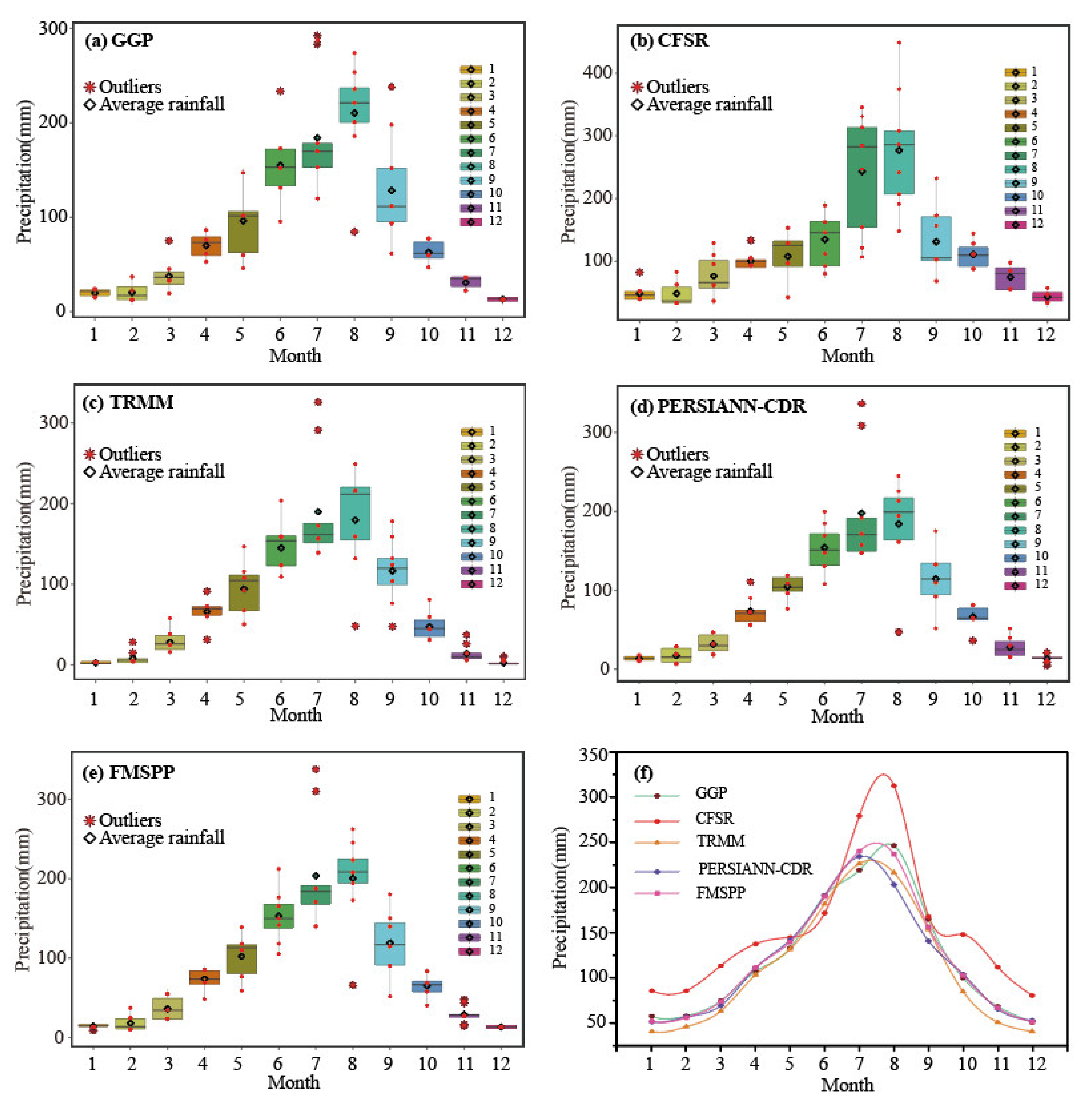
4.1. Temporal Evaluation of SPPs and FMSPP

Seven statistical indicators [40] were employed to quantitatively compare the performance of the original SPPs and FMSPP relative to GGP on the daily and monthly scales over the entire watershed. The indicators were the correlation coefficient (CC), root mean squared error (RMSE), mean error (ME), relative bias (BIAS), probability of detection (POD), false alarm ratio (FAR), and critical success index (CSI). The CC described the potential linear correlation between SPP and GGP, ranging from −1 to 1. The closer the CC value to 1, the more positively the SPP correlated with GGP. The RMSE, ME, and BIAS were introduced to describe the difference in the precipitation amount between the two rainfall products. Smaller absolute values of these three indexes meant minor discrepancies between SPP and GGP. The POD, FAR, and CSI were detectors for predicting rainfall occurrence on a daily scale. Higher POD and CSI and lower FAR corresponded to a higher ability to predict rainfall events.

As shown in

Table 5. Statistical analysis of SPPs and FMSPP over the whole watershed on a daily scale.

Precipitation Product	CC	RMSE (mm)	ME (mm)	BIAS (%)	POD	FAR	CSI
CFSR	0.72	4.44	1.02	35.6	0.92	0.17	0.83
TRMM	0.37	6.43	−0.35	−13.09	0.58	0.15	0.85
PERSIANN-CDR	0.36	6.41	−0.06	−2.9	0.68	0.23	0.77
FMSPP	0.57	4.92	−0.0004	−0.013	0.92	0.17	0.83

and Figure 6, the daily precipitation was mainly below 40 mm. CFSR had the highest CC of 0.72, the minimum RMSE of 4.44 mm, and the maximum POD of 0.92. However, its ME and BIAS were the largest, and both indexes were positive, revealing that precipitation was overestimated. The CC of TRMM and PERSIANN-CDR was 0.37 and 0.36, respectively; meanwhile, the RMSE of TRMM and PERSIANN-CDR was 6.43 and 6.41, respectively. Both the ME and BIAS for these two precipitation products were negative, indicating the underestimation of rainfall. The POD and CSI of the three original SPPs were relatively high, distributed in the range of 0.58–0.92 and 0.77–0.85, respectively, and the FAR was as low as 0.23. The values of CC and RMSE for FMSPP fell within the range obtained from the original SPPs. What is more, its POD, FAR, and CSI were the same as CFSR, which was the best. Additionally, the absolute values of ME and BIAS for FMSPP were the smallest (close to 0). Overall, FMSPP performed relatively well compared with the original SPPs on a daily scale.

On the monthly scale (

Table 6. Statistical analysis of SPPs and FMSPP over the whole watershed on a monthly scale.

Precipitation Product	CC	RMSE (mm)	ME (mm)	BIAS (%)
CFSR	0.86	53.10	31.47	35.5
TRMM	0.97	21.39	−11.56	−13.09
PERSIANN-CDR	0.95	23.07	−2.46	−2.9
FMSPP	0.97	17.12	−0.011	−0.013

and Figure 7), the CC for FMSPP was the highest, and its RMSE was the smallest. Besides, the absolute values of ME and BIAS for FMSPP were close to 0. These results demonstrated that the performance of FMSPP was the best. CFSR presented the largest BIAS and ME. The CC for TRMM reached 0.97, followed by 0.95 of PERSIANN-CDR, and 0.86 of CFSR. Compared to FMSPP, the RMSE for TRMM and PERSIANN-CDR increased slightly, and that for CFSR almost tripled. FMSPP showed analogous rainfall probability density distributions to TRMM and PERSIANN-CDR. By comparison, CFSR allocated more rainfall in the scope of 100–150 mm. Moreover, The ME and BIAS of CFSR were positive, and those for TRMM, PERSIANN-CDR, and FMSPP were negative, illustrating that CFSR overestimated rainfall while TRMM and PERSIANN-CDR underestimated rainfall. This result was consistent with the conclusion on the daily scale.

Figure 8 displayed the variation law of average monthly rainfall of the five precipitation products from 2000 to 2008. Most of the annual precipitation was allocated during the wet season from June to September. In contrast, the dry season from November to February accounted for a mere portion of the annual rainfall. The distribution of FMSPP, TRMM, and PERSIANN-CDR was consistent with that of the GGP. Outliers of these four precipitation products were scattered on the maximum side in July and scattered on the minimum side in August. CFSR had no outliers and significantly overestimated the rainfall in these two months. TRMM slightly underestimated the rainfall during the dry season.

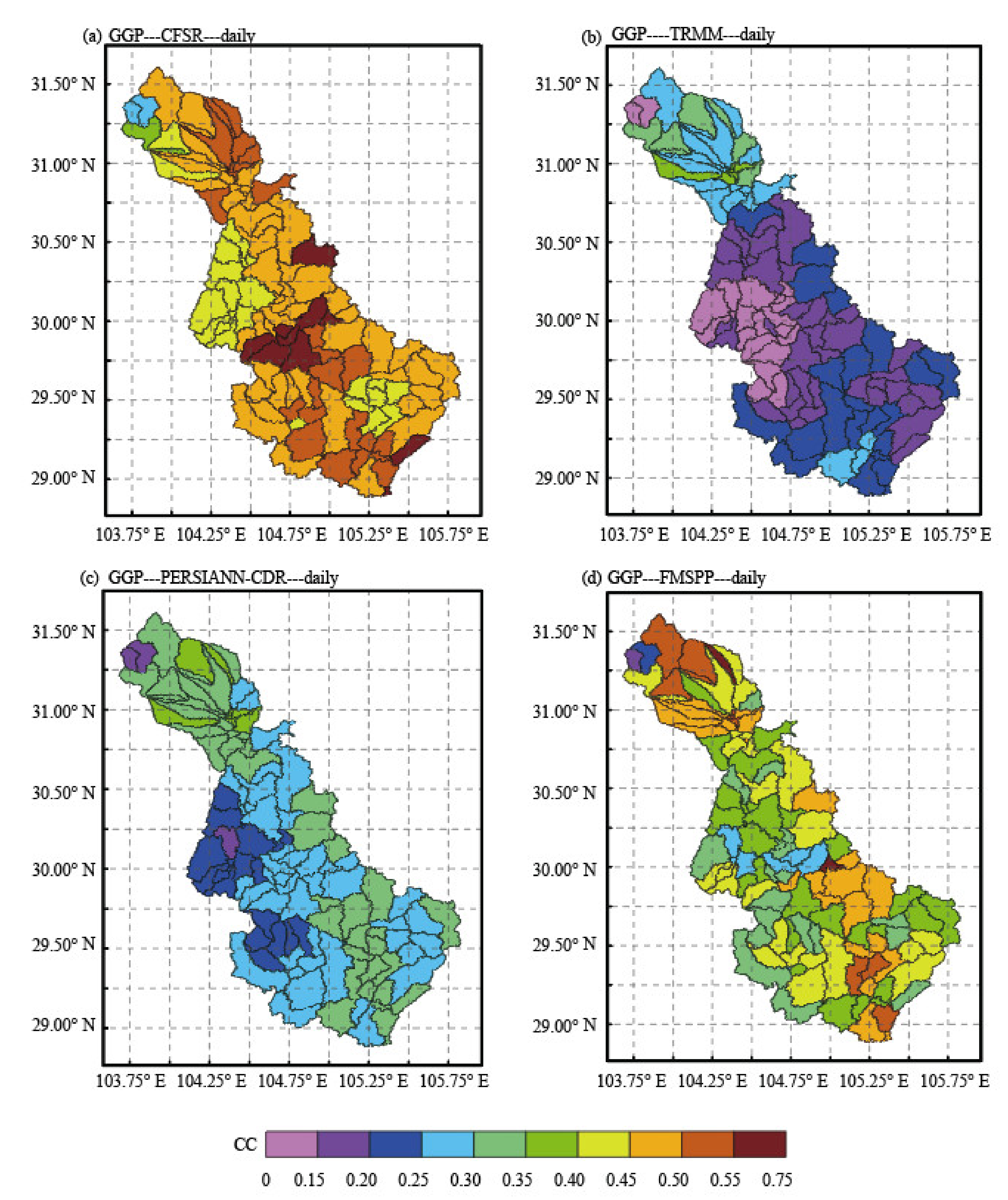
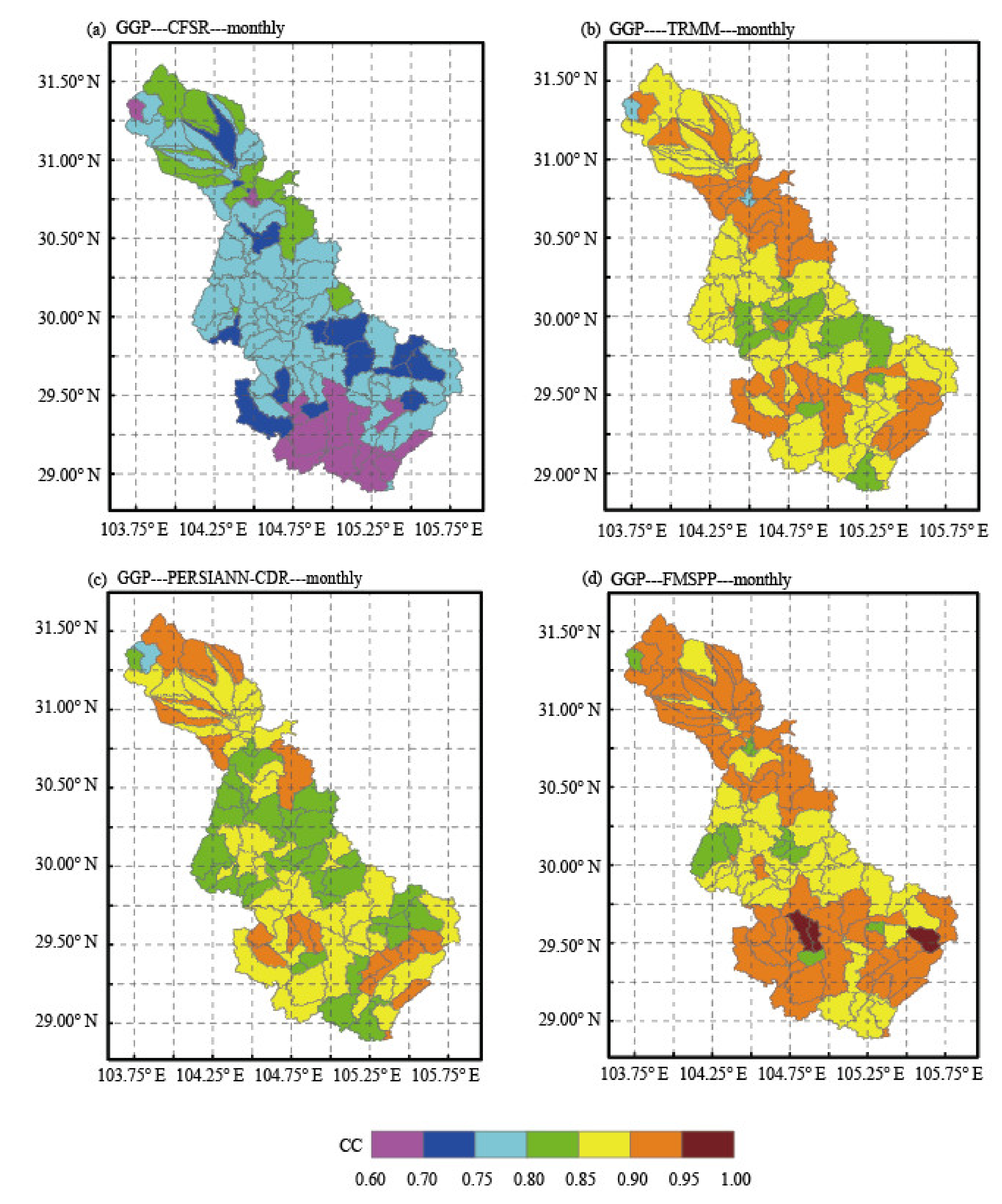
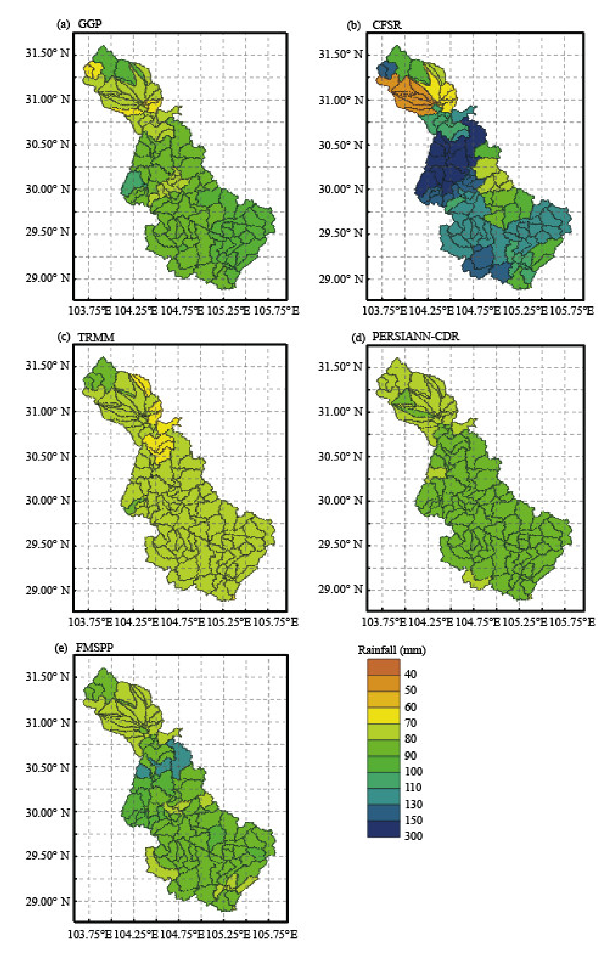
4.2. Spatial Evaluation of SPPs and FMSPP

Figure 9 and Figure 10 show the spatial variation of the CC for the original SPP and FMSPP on daily and monthly scales. In terms of the daily-scale CC, CFSR was around 0.5, except for a small amount of terrain in the northern mountainous area with the CC of 0.3. The correlation coefficients for PERSIANN-CDR over most subbasins were around 0.3 except for a minor portion of northern and midwestern regions. That for TRMM varied distinctly from 0.3 in the north to 0.2 in the south. The CC for FMSPP improved remarkably compared with TRMM and PERSIANN-CDR, with most of the area within the range of 0.3–0.6. On the monthly scale, the CC for each precipitation product was improved significantly in all sub-basins. FMSPP had the highest correlation in contrast with the other three SPPs. Its CC changed in the range of 0.84–0.96. TRMM and PERSIANN-CDR were slightly inferior to FMSPP. Their CCs in most areas ranged from 0.80 to 0.9. That for CFSR was below 0.8.

Regarding the variation of average monthly and annual rainfall (Figure 11 and Figure 12), the four precipitation products all captured the spatial features of less water in the north than in the south. The monthly and annual rainfall of FMSPP in most subbasins was below 100 and 1200 mm, respectively. This result was close to GGP. In addition, the three precipitation products other than CFSR showed a gradually increasing trend from north to south. CFSR was very different in the northern and midwestern regions—precipitation was slightly underestimated in the north and significantly overestimated in the midwest. Specifically, the monthly precipitation and annual precipitation of GGP in the north were about 65 mm and 800 mm, respectively, and those of the CFSR were about 50 mm and 700 mm, respectively. In the central and western regions, the monthly precipitation and annual precipitation of GGP were 95 mm and 1100 mm, and those of the CFSR were 200 mm and 2500 mm, respectively. Note that these two areas were the transitional zones from the mountainous area to the plain. The rainfall was more significantly affected by topographical factors in these two areas than in the southern plain [41]. The notable deviation of CFSR from GGP illustrated that the CFSR was prone to more considerable error in complex terrain than the TRMM and PERSIANN-CDR in this basin.

4.3. Evaluation of the Hydrological Performance of Different Precipitation Products

This part mainly evaluated the hydrological applicability of FMSPP and compared its performance with that of other precipitation products. All precipitation products used the same set of parameters when driving the SWAT model to reduce the propagation of uncertainty caused by the model structure. In this paper, we adopted high-precision GGP to drive the hydrological model; 1980–1992 and 1993–1999 were used as the calibration period and validation period, respectively. The simulated monthly streamflow was calibrated and validated by the measurements at the three hydrological stations. After that, 2000–2008 was selected as the evaluation period to evaluate the accuracy of each precipitation product in streamflow prediction. The warm-up period was 1998–1999. The coefficient of determination (R²), Nash Sutcliff (NS), and Percent Bias (PBIAS) were used to evaluate the hydrological performance.

The optimal value of R² and NS is 1. The better simulations receive higher values of R² and NS. PBIAS is used to characterize whether the mean magnitude of the modeled streamflow is higher or lower than the measured one. If it is less than 0, the streamflow is overestimated, and otherwise, underestimated.

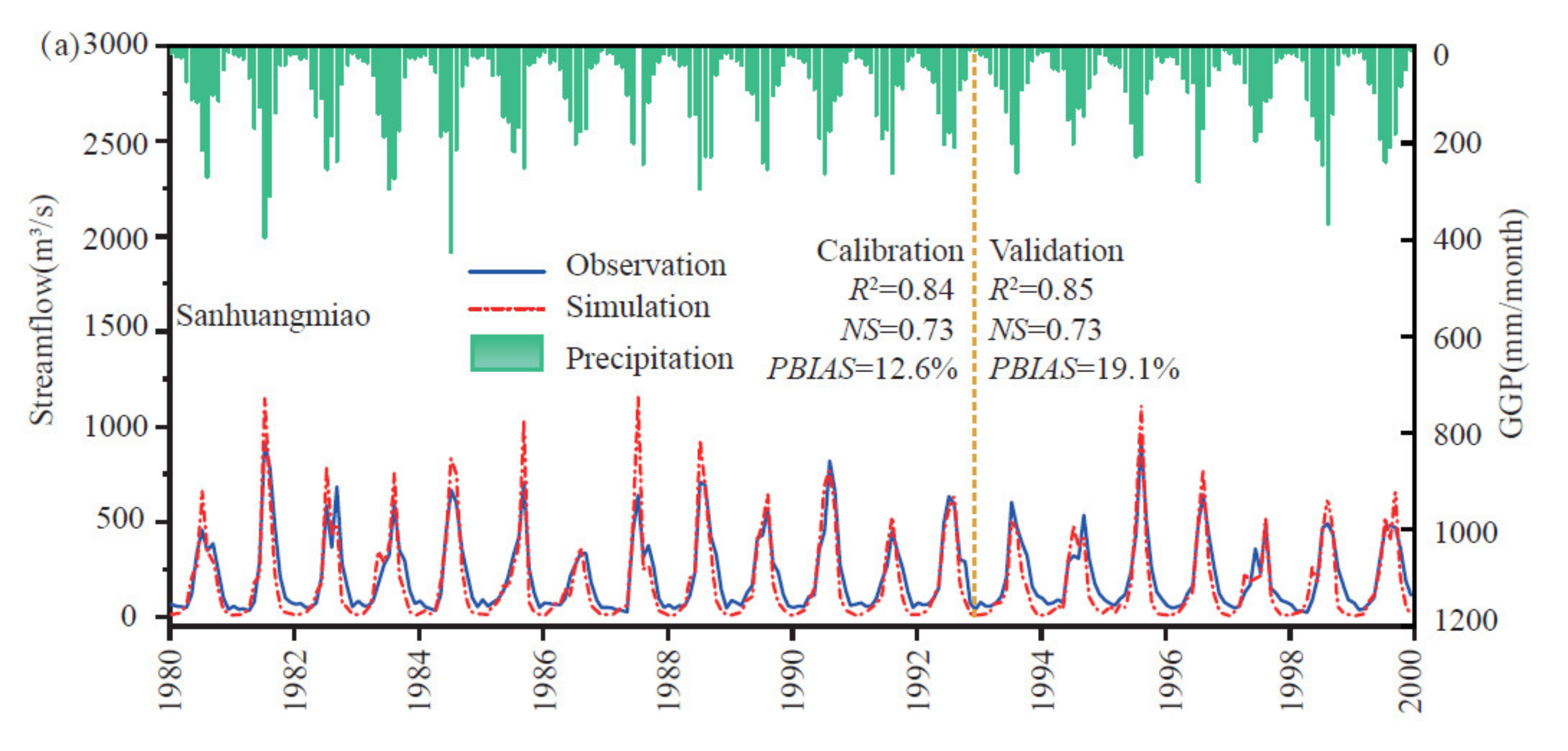
4.3.1. Calibration and Validation

Based on the Sequential Uncertainty Fitting (SUFI) algorithm embedded in the SWAT Calibration Uncertainty Programs (SWAT-CUP), the Latin hypercube method [42] was utilized to sample each parameter value within a specific range, and NS was used as the objective function to find the optimal parameter set.

Table 7. Global sensitivity analysis of the parameters and the corresponding optimal values.

Parameter Name	Rank	t-Value	t-Value	Fitting Value	Min Value	Max Value
R__CN2.mgt	1	4.83	0.0005	0.18	−0.2	0.2
V__ALPHA_BNK.rte	2	4.12	0.001	0.33	0	1
V__CH_N2.rte	3	−2	0.05	0.09	0	0.3
V__GWQMN.gw	4	1.79	0.08	0.86	0	2
V__GW_DELAY.gw	5	−1.19	0.24	210.6	30	450
V__CH_K2.rte	6	−0.84	0.41	56.25	5	130
V__ESCO.hru	7	−0.65	0.52	0.85	0.8	1
V__ALPHA_BF.gw	8	0.46	0.65	0.71	0	1
R__SOL_AWC.sol	9	−0.29	0.78	0.14	−0.2	0.4
R__SOL_BD.sol	10	−0.18	0.86	−0.45	−0.5	0.6
R__SOL_K.sol	11	−0.1	0.92	0.3	−0.8	0.8
V__SFTMP.bsn	12	−0.1	0.92	0.7	−5	5
V__GW_REVAP.gw	13	−0.03	0.98	0.01	0	2

Notes: V means that the current parameter value is to be replaced by a given value; R represents that the current parameter value is to be multiplied by (1 + a given value).

shows the range of each parameter [43], the optimal parameter set, and the global sensitivity analysis results. The t-value was employed to identify the significance of the parameter, and the p-value determined whether to reject the null hypothesis (a rejection of the hypothesis meant that the parameter had a significant impact on the objective function value). The global sensitivity analysis was relative to one-at-a-time sensitivity analysis, and it signified the alteration of the objective function value resulting from a parameter change. The more the objective function value changed, the more sensitive the objective function was to the parameter, corresponding to a higher t-value and a lower p-value. As shown in Figure 13 and Table 7, the most sensitive parameter was the initial SCS runoff curve for moisture condition Ⅱ (CN2), then base flow alpha-factor (ALPHA_BNK), followed by manning’s n value for the main channel (CH_N2). For the meaning of other parameters involved in the figure and table, please refer to [44].

The simulated runoff during the calibration period matched well with the runoff measured at the three hydrological stations (

Table 8. Results of the evaluation indexes in the calibration and validation periods for hydrological modeling.

Index	Station	Calibration	Validation
R2	Sanhuangmiao	0.84	0.85
	Dengyinyan	0.90	0.91
	Lijiawan	0.93	0.91
NS	Sanhuangmiao	073	0.73
	Dengyinyan	0.88	0.85
	Lijiawan	0.93	0.90
PBIAS (%)	Sanhuangmiao	12.6	19.1
	Dengyinyan	10.3	18.4
	Lijiawan	−2.7	−5.1

and Figure 14). The evaluation indexes NS, R², and PBIAS ranged from 0.73 to 0.93, 0.84 to 0.93, and −2.7% to 12.6%, respectively. In the validation period of 1993 to 1999, the simulation performance decreased marginally; NS and R² reduced slightly (0.1–0.2), and PBIAS almost doubled. Overall, the performance could be evaluated as “good” according to the SWAT performance rating criteria proposed in the literature [38].

4.3.2. Performance Comparison of SWAT Model Forced by Different Precipitation Products

During the evaluation period, the monthly streamflow measured and simulated at the Lijiawan hydrological station was used to compare the performance of different precipitation products in driving the SWAT model for monthly runoff prediction. Note that the streamflow measurements from 2005 to 2006 were not collected. The order of months labeled on the x-axis in Figure 15 was done in a consecutive way. Judging from the evaluation indicators in

Table 9. Comparison of monthly streamflow evaluation indexes of the five precipitation products from 2000 to 2008.

Precipitation Product	Evaluation Index
	R2	NS	PBIAS (%)
GGP	0.80	0.78	−2.9
CFSR	0.60	0.40	−29.6
TRMM	0.80	0.70	10.3
PERSIANN-CDR	0.68	0.65	−6.2
FMSPP	0.84	0.83	−1.9

and Figure 15, one could find that the PBIAS of the three precipitation products other than TRMM was smaller than 0, suggesting that the simulated streamflow was larger than the measured values. Specifically, the simulated discharge of GGP performed well with the indexes R² of 0.8 and NS of 0.78. R². The R² and NS for TRMM were very close to those of GGP, with values of 0.8 and 0.70, respectively, but its PBIAS was positive (10.3%), indicating that the modeled streamflow for TRMM was smaller than the measurements. The CFSR underestimated the streamflow in July 2002 and 2003 and notably overestimated the streamflow in July after 2004. Besides, CFSR had the smallest R² and NS, which were 0.60 and 0.40, respectively. In conclusion, the simulation result of CFSR was not as good as the other four precipitation products. The R² and NS for FMSPP were 0.84 and 0.83, respectively, close to those for GGP and TRMM (identified to perform well). Moreover, its PBIAS was the smallest among all the precipitation products, at only −1.9%, demonstrating its best performance. Therefore, FMSPP could drive the SWAT model successfully and improve monthly runoff prediction.

5. Discussion

The rainfall deviations of the three original SPPs and FMSPP from GGP are depicted in Figure 11 and Figure 12. The spatial distribution of TRMM, PERSIANN-CDR, and FMSPP is approximate to GGP over the sub-basins, whereas CFSR has the largest deviation from GGP. Besides, SPPs and FMSPP show a trend of underestimation in the south compared with GGP, while the spatial feature in the north is more complicated because of partial underestimation and overestimation. The western edge and midwest are mountainous areas and transitional zones, over where the rainfall bias is higher than that of the southern plain, particularly for CFSR. The CC values show the opposite pattern (Figure 9 and Figure 10). This result is consistent with the previous studies that satellite-based precipitation is more reliable in plain than in complex mountainous regions [21,45,46]. Note that, in addition to the reduced performance of SPPs in mountainous regions, the nature of the precipitation is also important. The study area is dominated by monsoonal rainfall, which tends to occur in large-scale systems that can be detected easily by relatively coarse-resolution satellite data. For basins in which, for example, convective rainfall is dominant, the performance of satellite-based precipitation measurement is likely to be worse.

In our study basin, we have a dense network of in-situ precipitation stations, and GGP naturally becomes the main accurate source of FMSPP. Just because of this, the analysis result of satellite precipitation products is hence more reliable. As shown in the spatial-temporal analysis and the hydrological modeling results, the performance of TRMM and PERSIANN-CDR is satisfactory. These good SPPs contribute some accuracy to the FMSPP; that is why FMSPP performs better than GGP. The results obtained in our study basin can provide a good reference to the data-sparse basin. If there are no in-situ stations, or the in-situ stations are too sparse, making the in-situ precipitation an unreliable source for the data-sparse basin, one can take the ‘most accurate satellite precipitation’ as the benchmark. This benchmark can be determined by referring to similar basins with rich in-situ stations. In that scenario, all the other possible precipitation sources, including the sparse in-situ precipitation, should be compared with the selected precipitation source. Therefore, the fusion method should be valid for the data-sparse region and can effectively reduce the uncertainty induced by multiple precipitation sources.

As mentioned in the literature [21], the hydrological performance of different SPPs in a particular basin may not apply to other basins with different characteristics. Different satellite products may perform distinctively in diverse regions. It is improper to judge which precipitation product is absolutely superior to the others based on the performance of the precipitation in a specific basin [47,48]. MIDSM-CCBWA proposed in this paper can dynamically integrate multi-source gauge-satellite precipitation at different sub-basins. This methodology effectively brings down the bias induced by the random application of a single satellite precipitation source to different regions and also maintains the characteristics of high-precision in-situ precipitation. Hence, the FMSPP has a more general hydrologic applicability in the data-sparse region.

Figure 16 shows the probability density distribution of the monthly precipitation of the five precipitation products. Besides, the correlations and their confidence intervals between any two precipitation products are displayed in the figure. CFSR is less correlated with the other four precipitation products. Its Pearson CC with GGP, TRMM, PERSIANN-CDR, and FMSPP is 0.86, 0.84, 0.85, and 0.89, respectively. The CC for FMSPP against GGP reaches 0.97, whereas that between FMSPP and CFSR is 0.89, which reveals that the fused rainfall product can well preserve the characteristics of GGP and its correlation with CFSR (identified to perform worse) is comparatively weak.

The magnitude and spatial distribution of precipitation directly influence the accuracy of runoff prediction. Figure 17 exhibits the correlations and confidence intervals between the measured streamflow and the simulations obtained from the rainfall products. The probability density distribution of the measured streamflow and that of the simulated streamflow are also shown in this figure. The simulated runoff significantly correlates with the measured runoff. The Pearson CC is 0.92 for FMSPP, 0.90 for both GGP and TRMM, and 0.82 for PERSIANN. The simulation performance of CFSR is relatively poor, but its CC value still reaches 0.77. Overall, one needs to be cautious if CFSR is selected as the single rainfall source to simulate monthly runoff in this basin. The FMSPP presents the highest CC with the measured runoff.

The GGP is used to calibrate the model on the premise that the model parameters are stationary. During the evaluation period, the hydrological performance forced by each precipitation product is assessed by comparing the simulated monthly runoff with the measurements. According to the water balance equation, the amount of river flow depends on the water yield contributed by each sub-basin (or HRU). Water yield is mainly composed of three parts: surface flow, lateral flow, and groundwater flow. Figure 18 shows the CC of the different components of the water balance in the SWAT model simulated by each rainfall product. It can be deduced that the precipitation is significantly correlated with water yield, and the CC between precipitation and water yield for all the five rainfall products, i.e., GGP, CFSR, TRMM, PERSIANN-CDR, and FMSPP, is 0.93, 0.88, 0.91, 0.89, and 0.84, respectively.

However, various water balance components may contribute differently to water yield in different precipitation products; this may affect the simulated runoff. For example, surface runoff and lateral runoff are the main constituents of water yield for all the precipitation products, and their correlation with water yield can reach about 0.9. Groundwater flow does not contribute much to runoff generation in GGP, CFSR, and TRMM, while its correlation with water yield obtained in PERSIANN-CDR and FMSPP comes up to 0.66 and 0.76, respectively. The different contributions of groundwater flow to water yield modeled by different precipitation products are possibly due to the antecedent soil condition influenced by extreme flood events [49].

6. Conclusions

We propose the MIDSM-CCBWA fusion method to gain a more accurate areal rainfall FMSPP. The FMSPP was generated from an open database composed of multiple SPPs and GGP. In the case study based on the TJRB, the satellite precipitation sources involved in the database included CFSR, TRMM, and PERSIANN-CDR. Evaluation of each SPP and FMSPP at different spatio-temporal scales was performed over the TJRB. Then, the simulated streamflow forced by FMSPP, GGP, and each SPP was compared with the observations to evaluate their applicability to the hydrological modeling. The correlations and their confidence intervals between different precipitation products were further discussed, as well as the correlation of the water balance components in these precipitation products. This method can enhance the applicability of satellite precipitation products in hydrological models and improve the accuracy of hydrological forecasts by reducing the deviation caused by the uncertainty of precipitation sources. The main conclusions are as follows:

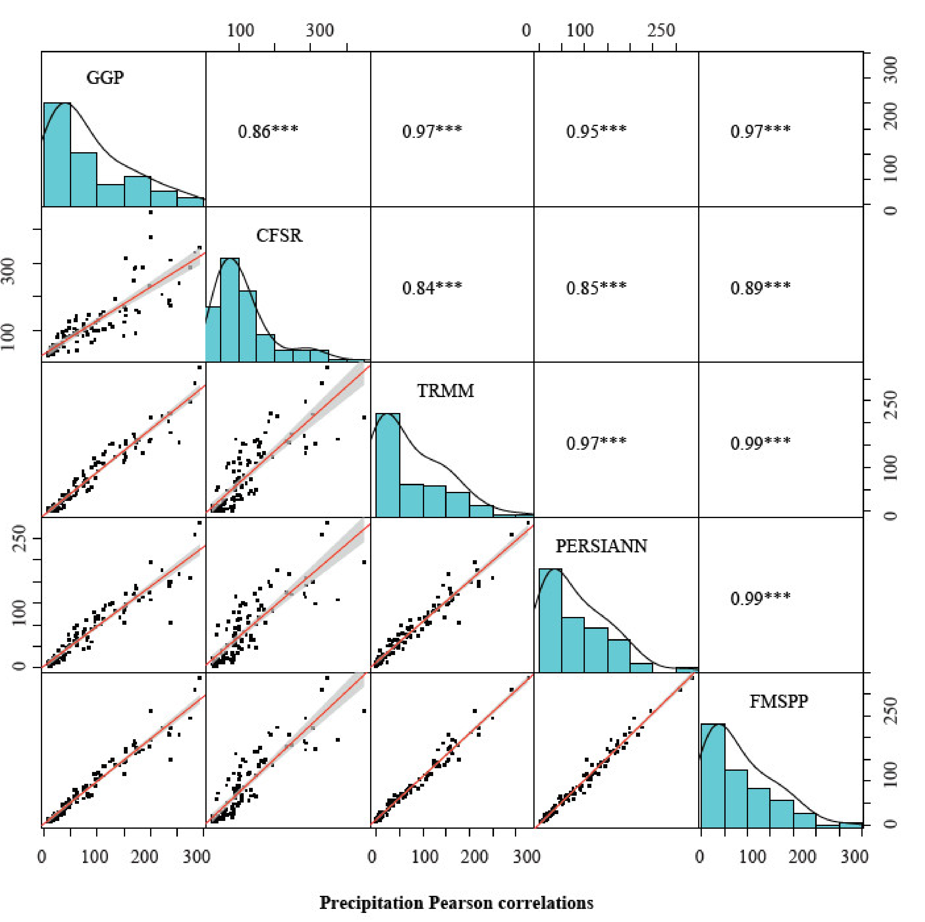
• FMSPP shows the maximum POD and minimum CSI, which proves that FMSPP can capture the occurrence of rainfall events very well. What is more, the absolute values of ME and BIAS for FMSPP are the smallest both on the daily and monthly scales over the watershed. Besides, the CC is significantly higher in most sub-basins on the monthly scale for FMSPP than the other three SPPs. Its CC changes in the range of 0.84–0.96. These results demonstrate that the performance of FMSPP is the best compared with the original SPPs.
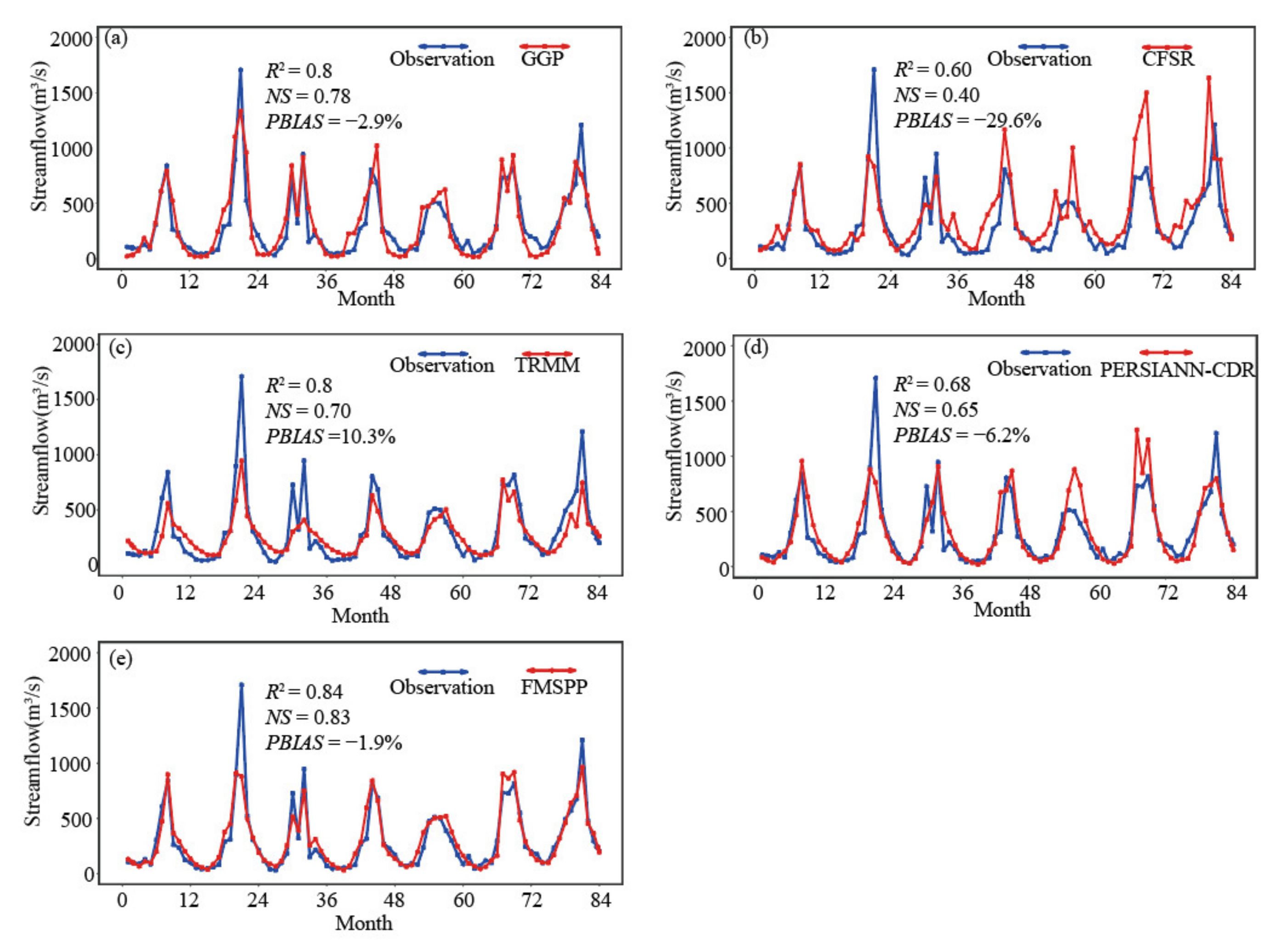
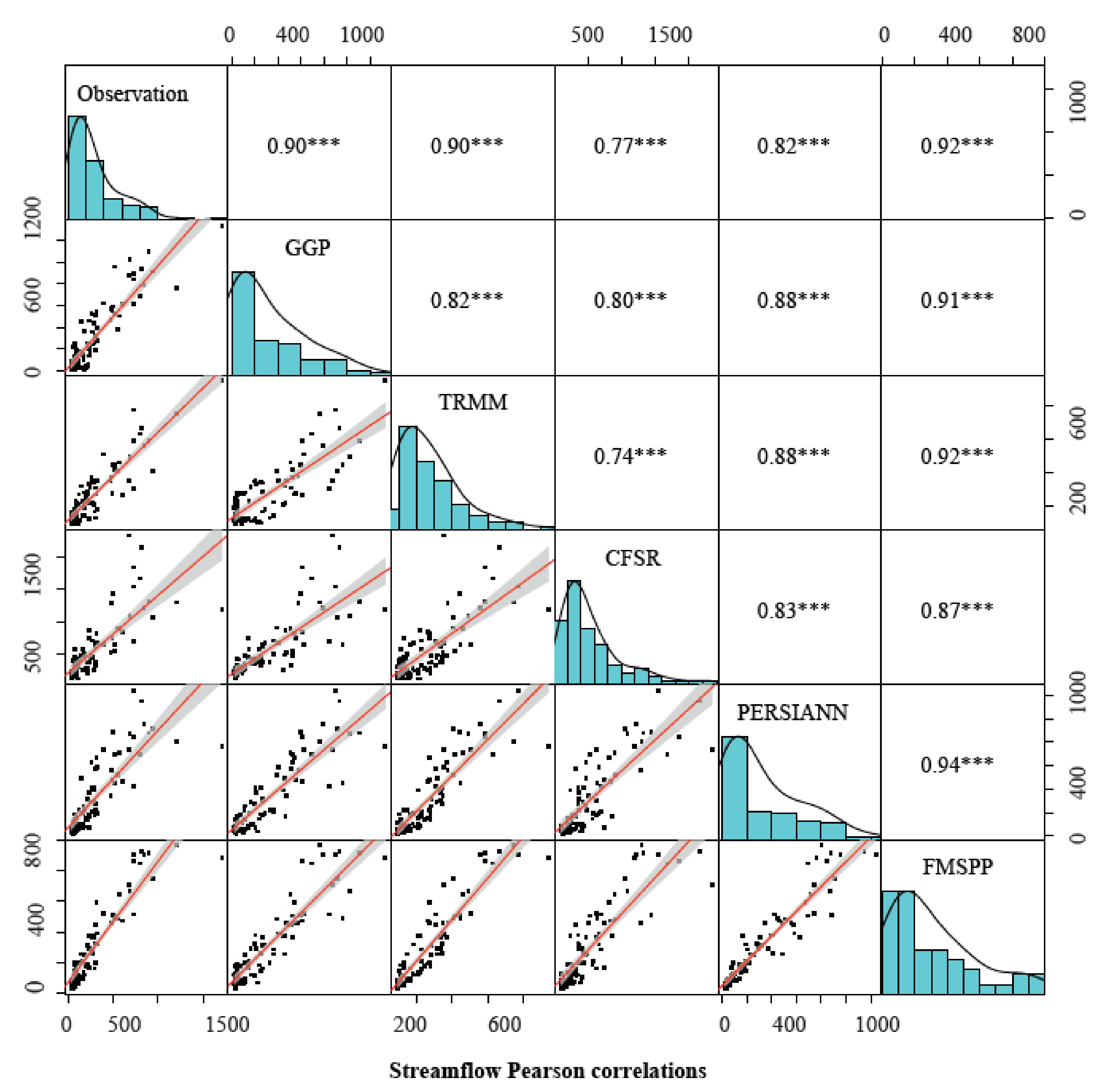
• Among the precipitation products, FMSPP shows the best simulation results, with R² and NS both being the largest, which are 0.83 and 0.84, respectively. Moreover, its PBIAS is the smallest, at only −1.9%. The hydrological performance of GGP and TRMM is good, followed by PERSIANN-CDR, whereas CFSR is unsatisfactory.
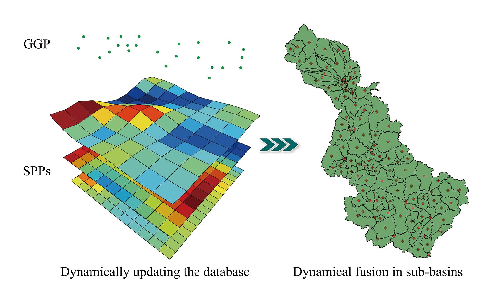
• The proposed MIDSM-CCBWA fusion method dynamically integrates multi-source gauge-satellite precipitation over different sub-basins and forms the FMSPP, which can effectively reduce the bias induced by the random application of a single precipitation source and improve the general applicability for streamflow simulation in the data-sparse region.
• FMSPP can preserve the characteristics of the precipitation source identified to perform well (e.g., GGP in the case study). It only has a relatively slight correlation with the precipitation source identified to perform worse (e.g., CFSR in this study).
• The rainfall deviation of SPPs from GGP over the mountainous areas on the northwest is higher than that of the southern plain, and the CC shows the opposite pattern in these areas. Thus, the satellite-based precipitation is generally more reliable in plain than in mountainous terrain for the study basin.

References

1. Yang, N.; Zhang, K.; Hong, Y.; Zhao, Q.H.; Huang, Q.; Xu, Y.S.; Xue, X.W.; Chen, S. Evaluation of the TRMM multisatellite precipitation analysis and its applicability in supporting reservoir operation and water resources management in Hanjiang basin, China. J. Hydrol. 2017, 549, 313–325. [Google Scholar] [CrossRef]
2. Hou, J.; Ye, A.; You, J.; Ma, F.; Duan, Q. An estimate of human and natural contributions to changes in water resources in the upper reaches of the Minjiang River. Sci. Total Environ. 2018, 635, 901–912. [Google Scholar] [CrossRef] [PubMed]
3. Zhang, Y.; Xia, J.; She, D.X. Spatiotemporal variation and statistical characteristic of extreme precipitation in the middle reaches of the Yellow River Basin during 1960–2013. Theor. Appl. Climatol. 2018, 135, 391–408. [Google Scholar] [CrossRef]
4. Xin, Z.H.; Li, Y.; Zhang, L.; Ding, W.; Ye, L.; Wu, J.; Zhang, C. Quantifying the relative contribution of climate and human impacts on seasonal streamflow. J. Hydrol. 2019, 574, 936–945. [Google Scholar] [CrossRef]
5. Jeong, C.; Lee, T. Copula-based modeling and stochastic simulation of seasonal intermittent streamflows for arid regions. J. Hydro Environ. Res. 2015, 9, 604–613. [Google Scholar] [CrossRef]
6. Lee, T. Multisite stochastic simulation of daily precipitation from copula modeling with a gamma marginal distribution. Theor. Appl. Climatol. 2017, 132, 1089–1098. [Google Scholar] [CrossRef]
7. Parisouj, P.; Mohebzadeh, H.; Lee, T. Employing Machine Learning Algorithms for Streamflow Prediction: A Case Study of Four River Basins with Different Climatic Zones in the United States. Water Resour. Manag. 2020, 34, 4113–4131. [Google Scholar] [CrossRef]
8. Beven, K.J.; Kirkby, M.J.; Freer, J.E.; Lamb, R. A history of TOPMODEL. Hydrol. Earth Syst. Sci. 2021, 25, 527–549. [Google Scholar] [CrossRef]
9. Gou, J.; Miao, C.; Duan, Q.; Tang, Q.; Di, Z.; Liao, W.; Wu, J.; Zhou, R. Sensitivity Analysis-Based Automatic Parameter Calibration of the VIC Model for Streamflow Simulations over China. Water Resour. Res. 2020, 56, e2019WR025968. [Google Scholar] [CrossRef] [Green Version]
10. Wu, Z.Y.; Xu, Z.G.; Wang, F.; He, H.; Zhou, J.H.; Wu, X.T.; Liu, Z.C. Hydrologic Evaluation of Multi-Source Satellite Precipitation Products for the Upper Huaihe River Basin, China. Remote Sens. 2018, 10, 840. [Google Scholar] [CrossRef] [Green Version]
11. Hiep, N.H.; Luong, N.D.; Viet Nga, T.T.; Hieu, B.T.; Thuy Ha, U.T.; Du Duong, B.; Long, V.D.; Hossain, F.; Lee, H. Hydrological model using ground- and satellite-based data for river flow simulation towards supporting water resource management in the Red River Basin, Vietnam. J. Environ. Manag. 2018, 217, 346–355. [Google Scholar] [CrossRef] [PubMed]
12. Zhu, H.L.; Li, Y.; Huang, Y.W.; Li, Y.C.; Hou, C.C.; Shi, X.L. Evaluation and hydrological application of satellite-based precipitation datasets in driving hydrological models over the Huifa river basin in Northeast China. Atmos. Res. 2018, 207, 28–41. [Google Scholar] [CrossRef]
13. Chao, L.J.; Zhang, K.; Li, Z.J.; Zhu, Y.L.; Wang, J.F.; Yu, Z.B. Geographically weighted regression based methods for merging satellite and gauge precipitation. J. Hydrol. 2018, 558, 275–289. [Google Scholar] [CrossRef]
14. Zhang, Y.Y.; Li, Y.G.; Ji, X.; Luo, X.; Li, X. Evaluation and Hydrologic Validation of Three Satellite-Based Precipitation Products in the Upper Catchment of the Red River Basin, China. Remote Sens. 2018, 10, 1881. [Google Scholar] [CrossRef] [Green Version]
15. Tang, G.Q.; Ma, Y.Z.; Long, D.; Zhong, L.Z.; Hong, Y. Evaluation of GPM Day-1 IMERG and TMPA Version-7 legacy products over Mainland China at multiple spatiotemporal scales. J. Hydrol. 2016, 533, 152–167. [Google Scholar] [CrossRef]
16. Cecinati, F.; Rico-Ramirez, M.A.; Heuvelink, G.B.M.; Han, D. Representing radar rainfall uncertainty with ensembles based on a time-variant geostatistical error modelling approach. J. Hydrol. 2017, 548, 391–405. [Google Scholar] [CrossRef] [Green Version]
17. Tang, G.Q.; Clark, M.P.; Papalexiou, S.M.; Ma, Z.Q.; Hong, Y. Have satellite precipitation products improved over last two decades? A comprehensive comparison of GPM IMERG with nine satellite and reanalysis datasets. Remote Sens. Environ. 2020, 240, 111697. [Google Scholar] [CrossRef]
18. Blacutt, L.A.; Herdies, D.L.; de Gonçalves, L.G.G.; Vila, D.A.; Andrade, M. Precipitation comparison for the CFSR, MERRA, TRMM3B42 and Combined Scheme datasets in Bolivia. Atmos. Res. 2015, 163, 117–131. [Google Scholar] [CrossRef] [Green Version]
19. Liu, X.M.; Yang, T.T.; Hsu, K.L.; Liu, C.M.; Sorooshian, S. Evaluating the streamflow simulation capability of PERSIANN-CDR daily rainfall products in two river basins on the Tibetan Plateau. Hydrol. Earth Syst. Sci. 2017, 21, 169–181. [Google Scholar] [CrossRef] [Green Version]
20. Ma, D.; Xu, Y.P.; Gu, H.T.; Zhu, Q.; Sun, Z.L.; Xuan, W.D. Role of satellite and reanalysis precipitation products in streamflow and sediment modeling over a typical alpine and gorge region in Southwest China. Sci. Total Environ. 2019, 685, 934–950. [Google Scholar] [CrossRef]
21. Zhu, Q.; Xuan, W.; Liu, L.; Xu, Y.-P. Evaluation and hydrological application of precipitation estimates derived from PERSIANN-CDR, TRMM 3B42V7, and NCEP-CFSR over humid regions in China. Hydrol. Process. 2016, 30, 3061–3083. [Google Scholar] [CrossRef]
22. Rahman, K.; Shang, S.; Shahid, M.; Li, J. Developing an Ensemble Precipitation Algorithm from Satellite Products and Its Topographical and Seasonal Evaluations Over Pakistan. Remote Sens. 2018, 10, 1835. [Google Scholar] [CrossRef] [Green Version]
23. Chen, Y.Y.; Huang, J.F.; Sheng, S.X.; Mansaray, L.R.; Liu, Z.X.; Wu, H.Y.; Wang, X.Z. A new downscaling-integration framework for high-resolution monthly precipitation estimates: Combining rain gauge observations, satellite-derived precipitation data and geographical ancillary data. Remote Sens. Environ. 2018, 214, 154–172. [Google Scholar] [CrossRef]
24. Lu, B.B.; Yang, W.B.; Ge, Y.; Harris, P. Improvements to the calibration of a geographically weighted regression with parameter-specific distance metrics and bandwidths. Comput. Environ. Urban Syst. 2018, 71, 41–57. [Google Scholar] [CrossRef]
25. Tang, G.Q.; Long, D.; Behrangi, A.; Wang, C.G.; Hong, Y. Exploring Deep Neural Networks to Retrieve Rain and Snow in High Latitudes Using Multisensor and Reanalysis Data. Water Resour. Res. 2018, 54, 8253–8278. [Google Scholar] [CrossRef] [Green Version]
26. Shen, Y.; Zhao, P.; Pan, Y.; Yu, J.J. A high spatiotemporal gauge-satellite merged precipitation analysis over China. J. Geophys. Res. Atmos. 2014, 119, 3063–3075. [Google Scholar] [CrossRef]
27. Zhu, Q.; Gao, X.; Xu, Y.-P.; Tian, Y. Merging multi-source precipitation products or merging their simulated hydrological flows to improve streamflow simulation. Hydrolog. Sci. J. 2019, 64, 910–920. [Google Scholar] [CrossRef]
28. Wu, H.C.; Yang, Q.L.; Liu, J.M.; Wang, G.Q. A spatiotemporal deep fusion model for merging satellite and gauge precipitation in China. J. Hydrol. 2020, 584, 124664. [Google Scholar] [CrossRef]
29. Ma, Y.Z.; Yang, Y.; Han, Z.Y.; Tang, G.Q.; Maguire, L.; Chu, Z.G.; Hong, Y. Comprehensive evaluation of Ensemble Multi-Satellite Precipitation Dataset using the Dynamic Bayesian Model Averaging scheme over the Tibetan plateau. J. Hydrol. 2018, 556, 634–644. [Google Scholar] [CrossRef]
30. Ur Rahman, K.; Shang, S.; Shahid, M.; Wen, Y. Hydrological evaluation of merged satellite precipitation datasets for streamflow simulation using SWAT: A case study of Potohar Plateau, Pakistan. J. Hydrol. 2020, 587, 125040. [Google Scholar] [CrossRef]
31. Guan, X.X.; Zhang, J.Y.; Yang, Q.L.; Tang, X.P.; Liu, C.S.; Jin, J.L.; Liu, Y.; Bao, Z.X.; Wang, G.Q. Evaluation of Precipitation Products by Using Multiple Hydrological Models over the Upper Yellow River Basin, China. Remote Sens. 2020, 12, 4023. [Google Scholar] [CrossRef]
32. Abbaspour, K.C.; Rouholahnejad, E.; Vaghefi, S.; Srinivasan, R.; Yang, H.; Kløve, B. A continental-scale hydrology and water quality model for Europe: Calibration and uncertainty of a high-resolution large-scale SWAT model. J. Hydrol. 2015, 524, 733–752. [Google Scholar] [CrossRef] [Green Version]
33. Jeong, H.-G.; Ahn, J.-B.; Lee, J.; Shim, K.-M.; Jung, M.-P. Improvement of daily precipitation estimations using PRISM with inverse-distance weighting. Theor. Appl. Climato. 2019, 139, 923–934. [Google Scholar] [CrossRef] [Green Version]
34. Xu, S.G.; Wu, C.Y.; Wang, L.; Gonsamo, A.; Shen, Y.; Niu, Z. A new satellite-based monthly precipitation downscaling algorithm with non-stationary relationship between precipitation and land surface characteristics. Remote Sens. Environ. 2015, 162, 119–140. [Google Scholar] [CrossRef]
35. Jia, S.; Zhu, W.; Lű, A.; Yan, T. A statistical spatial downscaling algorithm of TRMM precipitation based on NDVI and DEM in the Qaidam basin of China. Remote Sens. Environ. 2011, 115, 3069–3079. [Google Scholar] [CrossRef]
36. Iwasaki, H. NDVI prediction over mongolian grassland using GSMAP precipitation data and JRA-25/JCDAS temperature data. J. Arid Environ. 2009, 73, 557–562. [Google Scholar] [CrossRef]
37. Bao, Z.X.; Zhang, J.Y.; Wang, G.Q.; Guan, T.S.; Jin, J.L.; Liu, Y.L.; Li, M.; Ma, T. The sensitivity of vegetation cover to climate change in multiple climatic zones using machine learning algorithms. Ecol. Indic. 2021, 124, 107443. [Google Scholar] [CrossRef]
38. Pang, J.; Zhang, H.; Xu, Q.; Wang, Y.; Wang, Y.; Zhang, O.; Hao, J. Hydrological evaluation of open-access precipitation data using SWAT at multiple temporal and spatial scales. Hydrol. Earth Syst. Sci. 2020, 24, 3603–3626. [Google Scholar] [CrossRef]
39. Shukla, K.; Kumar, P.; Mann, G.S.; Khare, M. Mapping spatial distribution of particulate matter using Kriging and Inverse Distance Weighting at supersites of megacity Delhi. Sustain. Cities. Soc. 2020, 54. [Google Scholar] [CrossRef]
40. Tang, X.P.; Zhang, J.Y.; Gao, C.; Ruben, G.; Wang, G.Q. Assessing the Uncertainties of Four Precipitation Products for Swat Modeling in Mekong River Basin. Remote Sens. 2019, 11, 304. [Google Scholar] [CrossRef] [Green Version]
41. Liu, J.; Xia, J.; She, D.X.; Li, L.C.; Wang, Q.; Zou, L. Evaluation of Six Satellite-Based Precipitation Products and Their Ability for Capturing Characteristics of Extreme Precipitation Events over a Climate Transition Area in China. Remote Sens. 2019, 11, 1477. [Google Scholar] [CrossRef] [Green Version]
42. Shen, C.W.; Duan, Q.Y.; Gong, W.; Gan, Y.J.; Di, Z.H.; Wang, C.; Miao, S.G. An Objective Approach to Generating Multi-Physics Ensemble Precipitation Forecasts Based on the WRF Model. J. Meteorol. Res. 2020, 34, 601–620. [Google Scholar] [CrossRef]
43. Arnold, J.G.; Moriasi, D.N.; Gassman, P.W.; Abbaspour, K.C.; White, M.J.; Srinivasan, R.; Santhi, C.; Harmel, R.D.; Van Griensven, A.; Van Liew, M.W.; et al. SWAT: Model Use, Calibration, and Validation. Trans. ASABE 2012, 55, 1491–1508. [Google Scholar] [CrossRef]
44. Duan, Z.; Tuo, Y.; Liu, J.; Gao, H.; Song, X.; Zhang, Z.; Yang, L.; Mekonnen, D.F. Hydrological evaluation of open-access precipitation and air temperature datasets using SWAT in a poorly gauged basin in Ethiopia. J. Hydrol. 2019, 569, 612–626. [Google Scholar] [CrossRef] [Green Version]
45. Yilmaz, K.K.; Derin, Y. Evaluation of Multiple Satellite-Based Precipitation Products over Complex Topography. J. Hydrometeorol. 2014, 15, 1498–1516. [Google Scholar] [CrossRef] [Green Version]
46. Tian, Y.D.; Peters-Lidard, C.D. A global map of uncertainties in satellite-based precipitation measurements. Geophys. Res. Lett. 2010, 37. [Google Scholar] [CrossRef]
47. Maggioni, V.; Meyers, P.C.; Robinson, M.D. A Review of Merged High-Resolution Satellite Precipitation Product Accuracy during the Tropical Rainfall Measuring Mission (TRMM) Era. J. Hydrometeorol. 2016, 17, 1101–1117. [Google Scholar] [CrossRef]
48. Sun, Q.H.; Miao, C.Y.; Duan, Q.Y.; Ashouri, H.; Sorooshian, S.; Hsu, K.-L. A review of global precipitation data sets: Data sources, estimation, and intercomparisons. Rev. Geophys. 2018, 56, 79–107. [Google Scholar] [CrossRef] [Green Version]
49. Solano-Rivera, V.; Geris, J.; Granados-Bolaños, S.; Brenes-Cambronero, L.; Artavia-Rodríguez, G.; Sánchez-Murillo, R.; Birkel, C. Exploring extreme rainfall impacts on flow and turbidity dynamics in a steep, pristine and tropical volcanic catchment. Catena 2019, 182, 104118. [Google Scholar] [CrossRef]
Figure 1. Hydrological and meteorological stations (a), DEM (b), land use (c), and soil (d) of the TJRB.
Remotesensing 13 02630 g001
Figure 2. Spatial distribution of different precipitation products.
Remotesensing 13 02630 g002
Figure 3. Schematic diagram of the complete fusing processes for constructing a new precipitation data point.
Remotesensing 13 02630 g003
Figure 4. Dynamical fusing process of all available datasets.
Remotesensing 13 02630 g004
Figure 5. Schematic diagram of the MIDSM model (the height of the red bar represents the NDVI value of the precipitation product, and the height of the green bar represents the NDVI value at the center point of the sub-basin).
Remotesensing 13 02630 g005
Figure 6. Statistical analysis of SPPs and FMSPP over the whole watershed on a daily scale: (a) CFSR, (b) TRMM, (c) PERISANN-CDR, and (d) FMSPP.
Remotesensing 13 02630 g006
Figure 7. Statistical analysis of SPPs and FMSPP against GGP on a monthly scale over the whole watershed: (a) CFSR, (b) TRMM, (c) PERISANN-CDR, and (d) FMSPP (the change in the color of the dots from cyan to red represents the change in the magnitude of the rainfall from small to large).
Remotesensing 13 02630 g007
Figure 8. Average monthly rainfall distribution of the five precipitation products during 2000–2008 over the whole watershed: (a) GGP, (b) CFSR, (c) TRMM, (d) PERSIANN-CDR, and (e) FMSPP. (f) Compares the average of the five precipitation products.
Remotesensing 13 02630 g008
Figure 9. Spatial distribution of correlation coefficients for SPPs and FMSPP on a daily scale from 2000 to 2008: (a) CFSR, (b) TRMM, (c) PERISANN-CDR, and (d) FMSPP.
Remotesensing 13 02630 g009
Figure 10. Spatial distribution of correlation coefficients for SPPs and FMSPP on a monthly scale from 2000 to 2008: (a) CFSR, (b) TRMM, (c) PERISANN-CDR, and (d) FMSPP.
Remotesensing 13 02630 g010
Figure 11. Spatial variation of average monthly rainfall during the period of 2000–2008 obtained from (a) GGP, (b) CFSR, (c) TRMM, (d) PERSIANN-CDR, and (e) FMSPP.
Remotesensing 13 02630 g011
Figure 12. Spatial variation of average annual rainfall during the period of 2000–2008 obtained from (a) GGP, (b) CFSR, (c) TRMM, (d) PERSIANN-CDR, and (e) FMSPP.
Remotesensing 13 02630 g012
Figure 13. Global sensitivity analysis results of the parameters used in this study.
Remotesensing 13 02630 g013
Figure 14. Monthly streamflow measured at the three hydrological stations and the simulation result from GGP from 1980 to 1999 (1980–1992 for calibration and 1993–1999 for validation): (a) Sanhuangmiao, (b) Dengyinyan, and (c) Lijiawan.
Remotesensing 13 02630 g014aRemotesensing 13 02630 g014b
Figure 15. Comparison of the monthly runoff between the observations and those simulated with the five precipitation products at Lijiawan hydrological station from 2000 to 2004 (Months 1–60) and 2007 to 2008 (Months 61–84): (a) GGP, (b) CFSR, (c) TRMM, (d)PERSIANN-CDR, and (e) FMSPP.
Remotesensing 13 02630 g015
Figure 16. The probability density distribution of the monthly precipitation of the five precipitation products. Their correlations and confidence intervals are also presented (‘***’ indicates the significance level).
Remotesensing 13 02630 g016
Figure 17. The probability density distribution of the measured streamflow and that of the streamflow simulated from different precipitation products. Their correlations and confidence intervals are also presented. (‘***’ indicates the significance level).
Remotesensing 13 02630 g017
Figure 18. Correlation analysis of water balance components simulated by the five precipitation products. (‘×’ indicates no significant correlation): (a) GGP, (b) CFSR, (c) TRMM, (d) PERSIANN-CDR, and (e) FMSPP.
Remotesensing 13 02630 g018