Article

Simulating Heat Stress of Coal Gangue Spontaneous Combustion on Vegetation Using Alfalfa Leaf Water Content Spectral Features as Indicators

1
Institute of Land Reclamation and Ecological Restoration, China University of Mining & Technology (Beijing), Beijing 100083, China
2
College of Information and Electrical Engineering, China Agricultural University, Beijing 100083, China
3
Jiangsu Key Laboratory of Crop Genetics and Physiology, Co-Innovation Center for Modern Production Technology of Grain Crops, Agricultural College, Yangzhou University, Yangzhou 225009, China
4
Department of Land Management, Zhejiang University, Hangzhou 310058, China
*
Author to whom correspondence should be addressed.
Remote Sens. 2021, 13(13), 2634; https://0-doi-org.brum.beds.ac.uk/10.3390/rs13132634
Submission received: 23 May 2021 / Revised: 28 June 2021 / Accepted: 1 July 2021 / Published: 5 July 2021
(This article belongs to the Section Remote Sensing in Agriculture and Vegetation)

Abstract

:
Vegetation heat-stress assessment in the reclamation areas of coal gangue dumps is of great significance in controlling spontaneous combustion; through a temperature gradient experiment, we collected leaf spectra and water content data on alfalfa. We then obtained the optimal spectral features of appropriate leaf water content indicators through time series analysis, correlation analysis, and Lasso regression analysis. A spectral feature-based long short-term memory (SF-LSTM) model is proposed to estimate alfalfa’s heat stress level; the live fuel moisture content (LFMC) varies significantly with time and has high regularity. Correlation analysis of the raw spectrum, first-derivative spectrum, spectral reflectance indices, and leaf water content data shows that LFMC and spectral data were the most strongly correlated. Combined with Lasso regression analysis, the optimal spectral features were the first-derivative spectral value at 1661 nm (abbreviated as FDS (1661)), RVI (1525,1771), DVI (1412,740), and NDVI (1447,1803). When the classification strategies were divided into three categories and the time sequence length of the spectral features was set to five consecutive monitoring dates, the SF-LSTM model had the highest accuracy in estimating the heat stress level in alfalfa; the results provide an important theoretical basis and technical support for vegetation heat-stress assessment in coal gangue dump reclamation areas.

Graphical Abstract

1. Introduction

The organic materials in coal gangue dumps can oxidize and generate heat, such that spontaneous combustion may occur when the rate of heat generation exceeds that of heat dissipation [1,2]. The spontaneous combustion of coal gangue dumps poses a serious threat to the environment and human safety. This spontaneous combustion, by releasing a large number of toxic and harmful gases and chemical [3], damages the surrounding soil and water environment in the mining area [4,5]. It may also cause geological disasters during the long-term stacking [6], resulting in human casualties. In 2005, a coal gangue hill in China, spontaneously ignited, resulting in the death of eight people and burns to 122 people [7]. Further, over 30 miners were killed in the Ukraine from an explosion due to spontaneous combustion of coal in 2014 [8]. Remediation of coal gangue dumps mainly involves land reclamation and ecological reconstruction to reduce the probability of spontaneous combustion and other disasters [9,10]. A warning of spontaneous combustion in coal gangue dump reclamation areas helps managers take effective and timely countermeasures. Remote sensing can be used for this purpose. Researching this type of monitoring has mostly focused on surface temperature and coal fire monitoring via thermal infrared sensing [11,12,13,14,15,16,17]. However, changes in surface temperature are greatly affected by climate, sunshine, and other factors, which cause high hysteresis in spontaneous coal fire monitoring and make it impossible to obtain reliable early warnings. It has been found that prior to spontaneous combustion in coal gangue dumps, there is an internal heat accumulation stage that can affect the growth of plants. In this stage, there is potential to gain an early warning based on the spectral responses of plants. By averting spontaneous combustion disasters, the ecological environments of mining areas can be fundamentally improved.
Heat accumulation inside gangue dumps increases the surface soil temperature, which can reduce root numbers, roots’ absorption of water and nutrients, and plant fresh weights [18]. High soil temperature is far more influential than high air temperature on plant growth [19]. At present, few studies have used remote sensing to monitor soil heat stress and have mainly focused on drought stress [20], waterlogging stress [21], high-temperature stress [22], disease stress, and heavy metal stress [23]. Plant environmental stress has been estimated directly or indirectly based on spectral features (such as frequency-domain transformation features [24], vegetation indexes [25]), physiological and biochemical parameters (such as plant water [26], the leaf area index [27], pigment content [28], and chlorophyll fluorescence parameters [29]).
The heat stress caused by internal spontaneous combustion may eventually evolve into a fire in coal gangue dump reclamation areas. In such scenarios, the monitoring of plant water status is an important factor in detecting temperature anomalies [30]. Remote sensing can monitor plant water content because plant water absorbs radiation in the near-infrared (750–1300 nm) and short-wave-infrared (1300–2500 nm) regions [31]. Research has found that equivalent water thickness (EWT [20]), live fuel moisture content (LFMC [32]), and the relative water content (RWC [33]) of leaves can better reflect vegetation water status. Currently, commonly used vegetation moisture inversion methods include radiation transfer model inversion [30,34,35], traditional regression models [36,37], and machine learning models [38]. Yebra et al. [39] used radiation transfer model inversion to estimate fuel moisture contents from MODIS reflectivity data and established a flammability index through logistic regression modeling to map fire risk in Australia. Yi et al. [40] reported that DR1647/DR1133 and DR1653/DR1687 (DR = first-order differential reflectance value) are the optimal indexes for estimating EWT and LFMC, respectively. Rodríguez-Pérez et al. [36] used near-ground hyperspectral data to estimate grape leaf water content and used ordinary least-squares regression (OLSR) and functional linear regression (FLR) modeling, finding that the FLR model centered at 1465 nm had the highest accuracy (R2 = 0.7, RMSE = 8.485). Krishna et al. [41] predicted RWC according to the water deficit stress status of rice genotypes based on spectral indices, multivariate techniques, neural network techniques, and existing water-band indices. They proposed new water-band indices—the ratio index (RI) and normalized difference ratio index (NDRI)—for this purpose. In previous studies, the water indicators obtained by remote sensing technology have been used to qualitatively analyze plant water condition over an entire monitoring period to determine environmental stress level on vegetation. However, the accuracy and timeliness of the results are usually insufficient.
In this paper, a long short-term memory network model based on spectral features is proposed to estimate heat stress. It simulates the temperature–gradient test of plant heat stress in coal gangue dump reclamation areas and monitors plant water condition based on hyperspectral remote sensing. This provides a new way to monitor spontaneous combustion in coal gangue dumps. This method considers temporal variation in the spectral features of water status in vegetation under environmental stress. It allows accurate diagnoses to be made as soon as possible and provides a new method of remote sensing monitoring of other environmental stresses.

2. Materials and Methods

2.1. Experimental Design

The simulation experiment was carried out in the autumn of 2020 at the potted proving ground of Yangzhou University, Yangzhou, China (119°25′ N, 32°23′ E). Yangzhou is in the transition zone between the humid subtropical monsoon climate and the temperate monsoon climate. It has four distinct seasons and abundant sunshine and rainfall. Alfalfa, a common herbaceous plant commonly used in the reclamation areas of coal gangue dumps, was selected as the experimental plant. The species used was Algonquin [42].
Seeds were sown on 10 September 2020 at a sowing density of 10 holes per pot and two seeds per hole. Ten seedlings per pot were grown to the three-leaf stage and harvested on 15 November 2020. The inner diameter of the bottom of the barrel was 20 cm, the inner diameter of the mouth was 28 cm, the height of the pots was 31.5 cm, and the empty barrel weighed 0.54 kg. Each barrel was loaded with 10 kg air-dried light loam and 5.28 g compound fertilizer with an N-P-K ratio of 15%:15%:15%. One kilogram of soil was used to cover the seeds after sowing. The first alfalfa crop took about 60 days to grow from the sowing to the flowering stage. The gradient experiment of heat stress was started on 16 October 2020. The experimental design consisted of one control group and five experimental groups (T1, T2, T3, T4, T5), and each group was replicated five times, as shown in Figure 1a. For the experimental groups, five heat sources of different temperature T (T1 = 60 °C, T2 = 90 °C, T3 = 120 °C, T4 = 150 °C, and T5 = 180 °C) were placed at a depth of 30 cm in the soil layer, which is the typical thickness of overlying soil used in reclamation projects [43] (Figure 1b). Each group was replicated five times, as shown in Figure 1a. The relative water content of all treated soils was controlled at about 60%.

2.2. Data Acquisition

2.2.1. Spectral Data

A portable ground object spectrometer (Spectra Vista Corporation SVC HR-1024I) was used to measure the spectral reflectance of alfalfa leaves. The spectral measurement range was 340–2500 nm, and the spectral sampling intervals were 1.5 nm (sampling range 350–1000 nm), 3.8 nm (sampling range 1000–1885 nm), and 2.5 nm (sampling range 1885–2500 nm). The resample interval was 1 nm. The measurements were synchronized with the heating. The first measurement was made on 16 October 2020, and then every 4 days, postponed on cloudy and rainy days. The spectral reflectance of leaves was measured between 10:00 and 14:00 on sunny and windless days. The spectral data were collected eight times until 15 November 2020. A standard whiteboard was used for calibration of measurements using a hand-held leaf spectrum detector with a light source. The middle adaxial part of a leaf sample was clamped to the detector to measure its spectrum. Each process measured three pots, and each pot was measured at six leaves, with the average taken as the processed alfalfa leaf spectrum reflectance. During the measurement process, standard whiteboard calibration was performed every 30 min.

2.2.2. Leaf Water Content

Leaf water content data were collected synchronously with spectral data. Three alfalfa plants samples were selected for each treatment and packed in self-sealing plastic bags to avoid water loss from the plants as much as possible. Samples were quickly brought back to the laboratory to weigh their fresh weight ( m f ) with a precision balance and manually measure their leaf area. Each treated fresh leaf was put into a beaker filled with distilled water and soaked for 24 h. After reaching a constant weight, the saturated fresh weight was measured ( m t ). Then, a blade was put into the paper bag, which was placed in an oven at 105 °C for 30 min, then the drying temperature was set at 80 °C for 48 h until the constant weight was attained, which was measured as the dry weight ( m d ). The leaf water content was calculated according to Equations (1)–(3):
L F M C = m f m d m d
where m f is the measured weight of fresh leaves, and m d is the weight of the same sample after drying.
E W T = m f m d A
where A is the leaf area.
R W C = m f m d m t m d
where m t is the measured saturation weight of the leaves.

2.3. Methods

2.3.1. Spectral Feature Construction

Raw spectral data processing: MATLAB 2017a (MathWorks, Natick, MA, USA) was used to average the spectral curves collected for each treatment in the heat-stress test to reduce the differences within groups. Then, a one-dimensional Gaussian filter was applied to the mean spectral curve along the spectrum direction to smooth it. The sliding window was set to 5, as shown in Figure 2 and Supplementary Figure S1.
First derivative spectrum: Differential processing of a spectrum can reduce the influence of background information such as field noise and soil on spectral data [44]. The direct difference method was used to calculate the first-derivative spectrum of spectral reflectance to highlight the target spectral features. Equation (4) was used to calculate the first derivative of the spectrum.
ρ ( λ i ) = [ ρ ( λ i + 1 ) ρ ( λ i 1 ) ] / 2 Δ λ
In the formula, λ i is the wavelength, ρ ( λ i ) and ρ ( λ i ) are the reflectance and first-derivative spectrum of the wavelength λ i , respectively, and Δ λ is the interval between the wavelength λ i 1 and λ i .
Spectral reflectance index: The spectral reflectance index was constructed using the two-band combination method of raw and first-derivative spectral reflectance and compared with the conventional index (Table 1). The two-band combination method included the ratio vegetation index ( R V I   ( λ 1 ,   λ 2 ) ), normalized difference vegetation index ( N D V I   ( λ 1 ,   λ 2 ) ), and difference vegetation index ( D V I   ( λ 1 ,   λ 2 ) ). These are commonly used in remote sensing monitoring. The selection range of any band combination was between 340 and 2500 nm, and their formulas [45] are as follows:
N D V I   ( λ 1 ,   λ 2 ) = ( R λ 1 R λ 2 ) / ( R λ 1 + R λ 2 )
R V I   ( λ 1 ,   λ 2 ) = R λ 1 / R λ 2
D V I   ( λ 1 ,   λ 2 ) = R λ 1 R λ 2
where λ 1 and λ 2 are wavelengths (nm), and R λ 1 and R λ 2 are the reflectances at wavelengths λ 1 and λ 2 , respectively, and λ 1 λ 2 .

2.3.2. Spectral Feature Selection

Correlation analysis: The Pearson correlation coefficient (Equation (8)) was used to correlate the spectral parameters (raw spectrum, first-derivative spectrum, and vegetation index) with plant leaf water content indicators (LFMC, EWT, and RWC). Pairwise analysis selected highly correlated spectral features in the appropriate band range.
r ( X , Y ) = C o v ( X , Y ) δ X δ Y
where C o v ( X , Y ) is the covariance of X and Y , δ X is the variance of X , and δ Y is the variance of Y .
Lasso regression: The Lasso (least absolute shrinkage operator) regression model was proposed by Robert in 1996 and has become an important regression model in the field of machine learning [54]. The method is a compression estimator that constructs a penalty function to obtain a relatively refined model. This makes it compress some regression coefficients; that is, the sum of the absolute value of the forcing coefficient is less than a fixed value. Through regularization, the regression coefficients of some independent variables are compressed to zero, then the variable selection is completed. At the same time, Lasso regression retains the advantage of subset contraction and is a biased estimation model (Equation (9)) for dealing with data with multicollinearity.
min β 0 , β ( 1 2 N i = 1 N ( y j β x i T β 0 ) + λ j = 1 p | β j | )
where N is the sample number, y j is the predicted true value, x i is the observed value, β 0 is the bias, β is the weight of the observed variable, and λ is a non-negative regularization parameter. λ j = 1 p | β j | is called L 1 regularization.

2.3.3. Assessment of Heat Stress by SF-LSTM

LSTM is a recurrent neural network (RNN) architecture used in the field of deep learning and was proposed by [55]. Unlike standard feedforward neural networks, LSTM has a feedback connection. It not only processes point datasets (such as images) but also processes data sequences. Compared with other deep learning algorithms, LSTM performs very well in processing regression or classification problems with time series feature data and is now widely used. The characteristics of temporal change in physiological parameters must be taken into account when estimating environmental stress level, and the influence of subjective qualitative analysis on the estimation accuracy should be avoided as far as possible. Therefore, in this paper, based on the multi-dimensional and multi-time-series characteristics of the test plant moisture indicators, Pytorch (Facebook AI Research, Menlo Park, CA, USA) was used to construct the artificial RNN SF-LSTM. Its structure is shown in Figure 3.
SF-LSTM is a neural network model based on bidirectional LSTM and uses spectral features as the input layer. The whole network is composed of an input layer, bidirectional LSTM layer, full connection layer, SoftMax layer, and classified output layer. At the lower left of Figure 3, the data structure of the input layer is enlarged. Inspired by image data processing, a three-dimensional matrix was constructed with dimensions of (1) spectral features, (2) time-series, and (3) stress level. The data structure of the input layer not only considers the calculation of various spectral features but also ensures that the data can be calculated according to the time series. At the same time, the multi-dimensional vector operation makes the calculation efficient. The core computing units, called memory cells, are zoomed in at the lower right of Figure 3. In the memory cells, “⊗” and “⊕” denote the dot product and matrix addition, respectively. The first step of the memory cell is to decide what information to discard from the cellular state. This decision is made by a sigmoid layer called the “forget gate”. It looks at h t 1 (the previous output) and X t (the current input) and outputs a number between 0 and 1 for each number in C t 1 (the previous state), where 1 represents total retention and 0 represents total deletion (Equation (10)). The next step is to decide what information to store in the cellular state. The sigmoid layer called the “input gate” decides, which values to update, and the next tanh layer creates a candidate vector C t (Equations (11) and (12)), which is added to the state of the cell and combined with C t 1 to create the updated value C t (Equation (13)). Finally, the “output gate” determines the output of the memory cells. The output value of h t is obtained by multiplying the output of a sigmoid layer with the normalized C t value of the tanh layer (Equations (14) and (15)).
f t = σ ( W f [ h t 1 , X t ] + b f )
i t = σ ( W i [ h t 1 , X t ] + b i )
C t = tanh ( W c [ h t 1 , X t ] + b c )
C t = f t C t 1 + i t C t
o t = σ ( W o [ h t 1 , X t ] + b o )
h t = o t tanh ( C t )
where σ is the logistic sigmoid function, W is the weight matrix, is a dot product, and b is a bias term.

2.3.4. Validation

The observed sample data for constructing the model were divided into a training set (segmentation scale = 0.8) and validation set (segmentation scale = 0.2). The coefficient of determination (R2) and root mean square error (RMSE) were used as indicators of its accuracy [26] (Equations (16) and (17)). Accuracy is defined as the degree of consistency between the model results and the true categories (Equation (18)). Ten-fold cross-validation was adopted for the training set [56].
R M S E = i = 1 n ( y ^ i y i ) 2 n
R 2 = 1 i = 1 n ( y ^ i y i ) 2 i = 1 n ( y ¯ i y i ) 2
A c c u r a c y = n c l a s s n × 100 %
where y i is the true value, y ^ i is the predicted value, y ¯ i is the mean value, n is the number of samples, and n c l a s s is the number of correctly classified samples.

3. Results

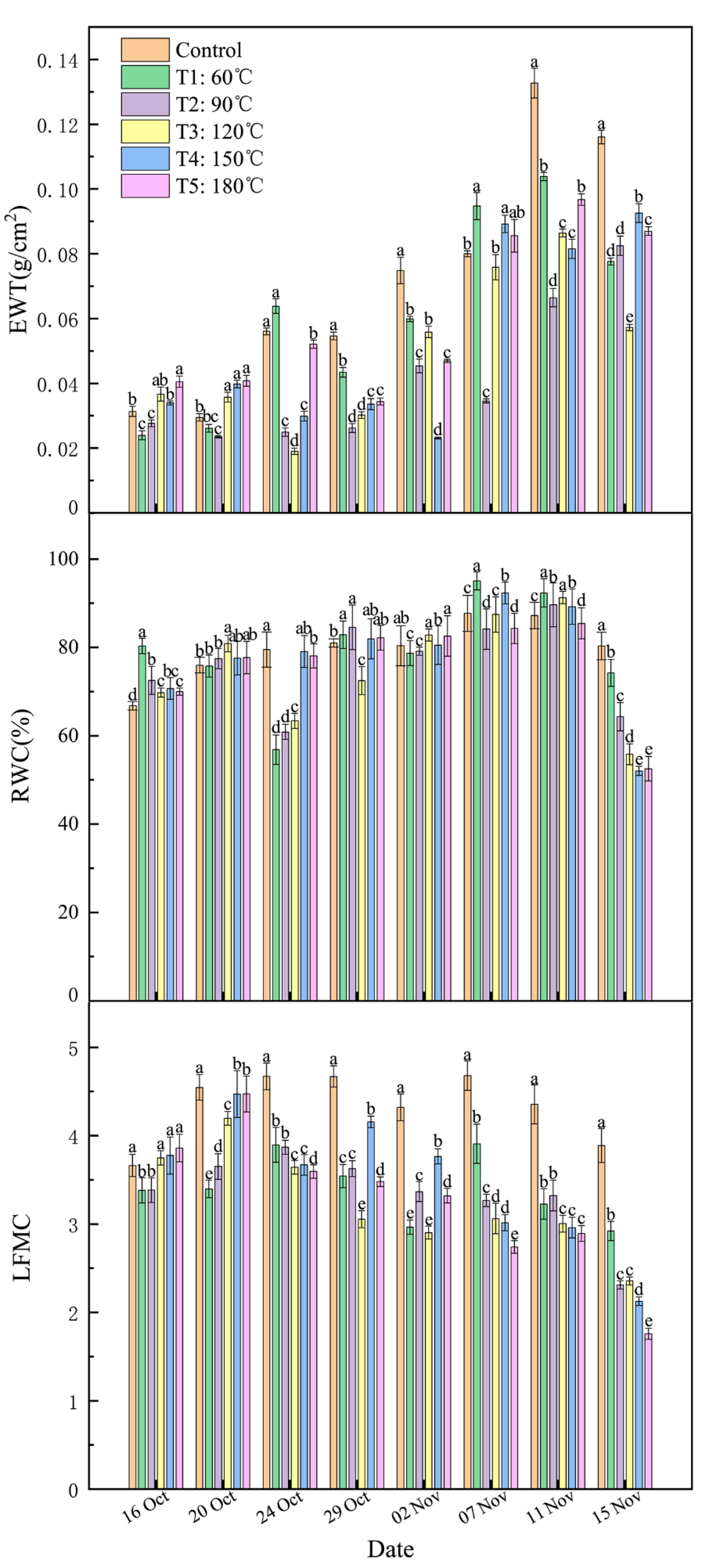
3.1. LFMC, EWT, and RWC Time Series Analysis

This study focused on alfalfa, a herbaceous plant commonly used in the reclamation areas of coal gangue dumps. The soil layer was heated on the day after the first data collection on 16 October, and leaf samples were collected eight times in total. Figure 4 shows the significant differences between treatments at each measurement date and the changes in LFMC, EWT, and RWC with time under different treatments. The soil layer was not heated when the soil was collected on 16 October. At this time, the growth trend in each alfalfa pot was similar, and the differences in LFMC, EWT, and RWC between each experimental group were non-significant. After heating, there was a lack of regularity in the significant differences in LFMC, EWT, and RWC between treatments within each measurement date. Therefore, we focused on analyzing the temporal trends of the three water indicators as follows. (1) EWT: All treatments showed an overall growth trend. The control group increased almost all the time, reaching the maximum value on 11 November before dropping slightly on 15 November. Apart from this overall trend, the EWTs of the other treatment of temperature groups showed different trends with no strong regularity over time. (2) RWC: The differences between groups on a particular date were small and the range of variation in RWC on different dates was relatively stable. On 7 and 11 November, the RWC of the control group and each experimental group peaked. On 15 November, the RWC of each treatment group declined, with a relatively large range of decreases. In general, there was no significant temporal trend in RWC between the control and experimental groups. (3) LFMC: After heating the soil layer, the LFMCs of the control group were significantly higher than those of the experimental groups on each monitoring date. The LFMCs of each experimental group showed gradually decreasing trends. In the late monitoring period, the LFMC decreased with increases in the temperature gradient on 7, 11, and 15 November and reached the lowest point on 15 November, exhibiting a clear decrease over time.
According to the results of water indicator monitoring and the above analysis, it is clear that LFMC is the best water indicator for reflecting heat stress in alfalfa. This is consistent with previous studies. LFMC is very sensitive to heat stress and is an important variable in many fire behavior prediction models and fire-risk indicators [39,57].

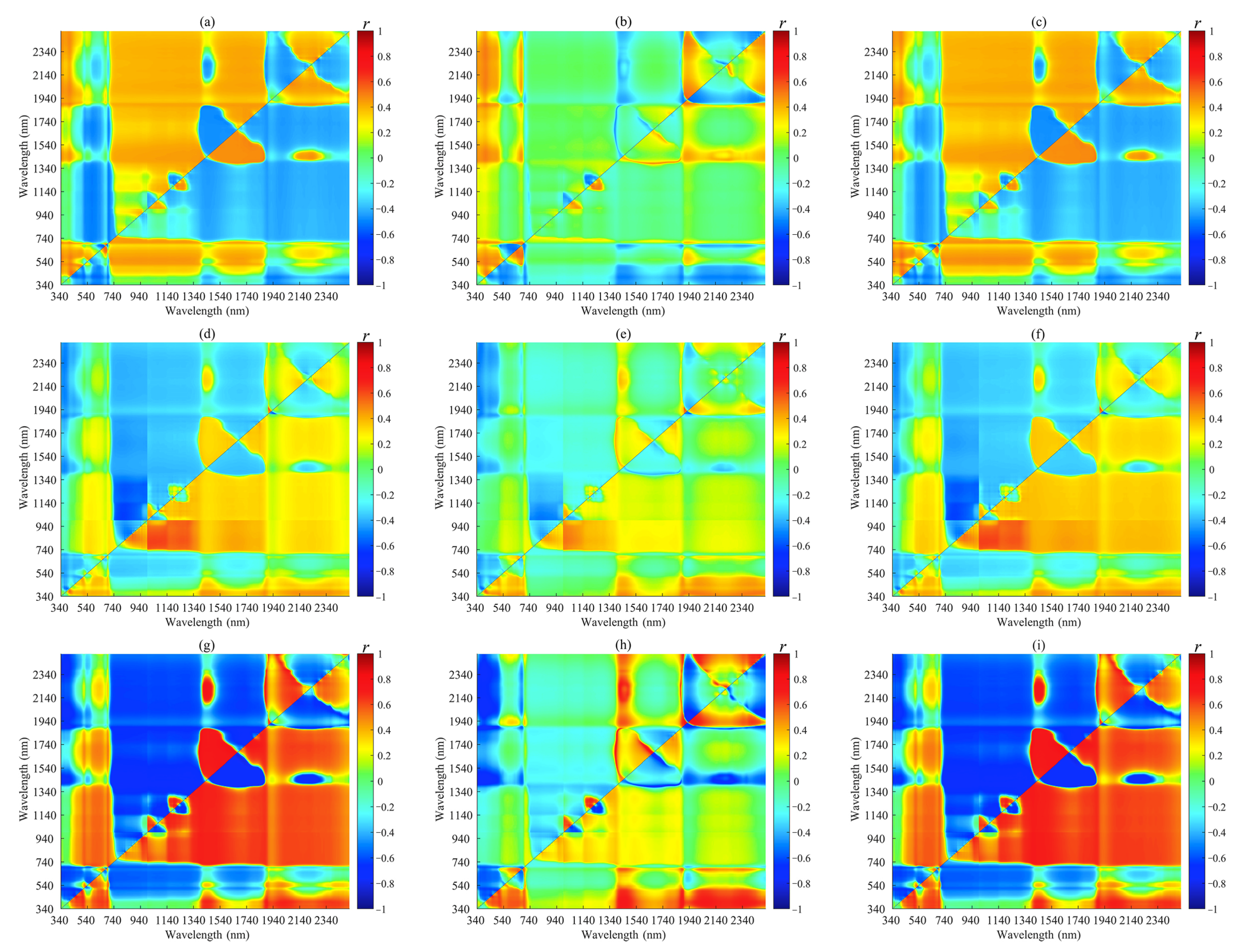
3.2. Correlation Analysis of Spectral Features and Leaf Water Content

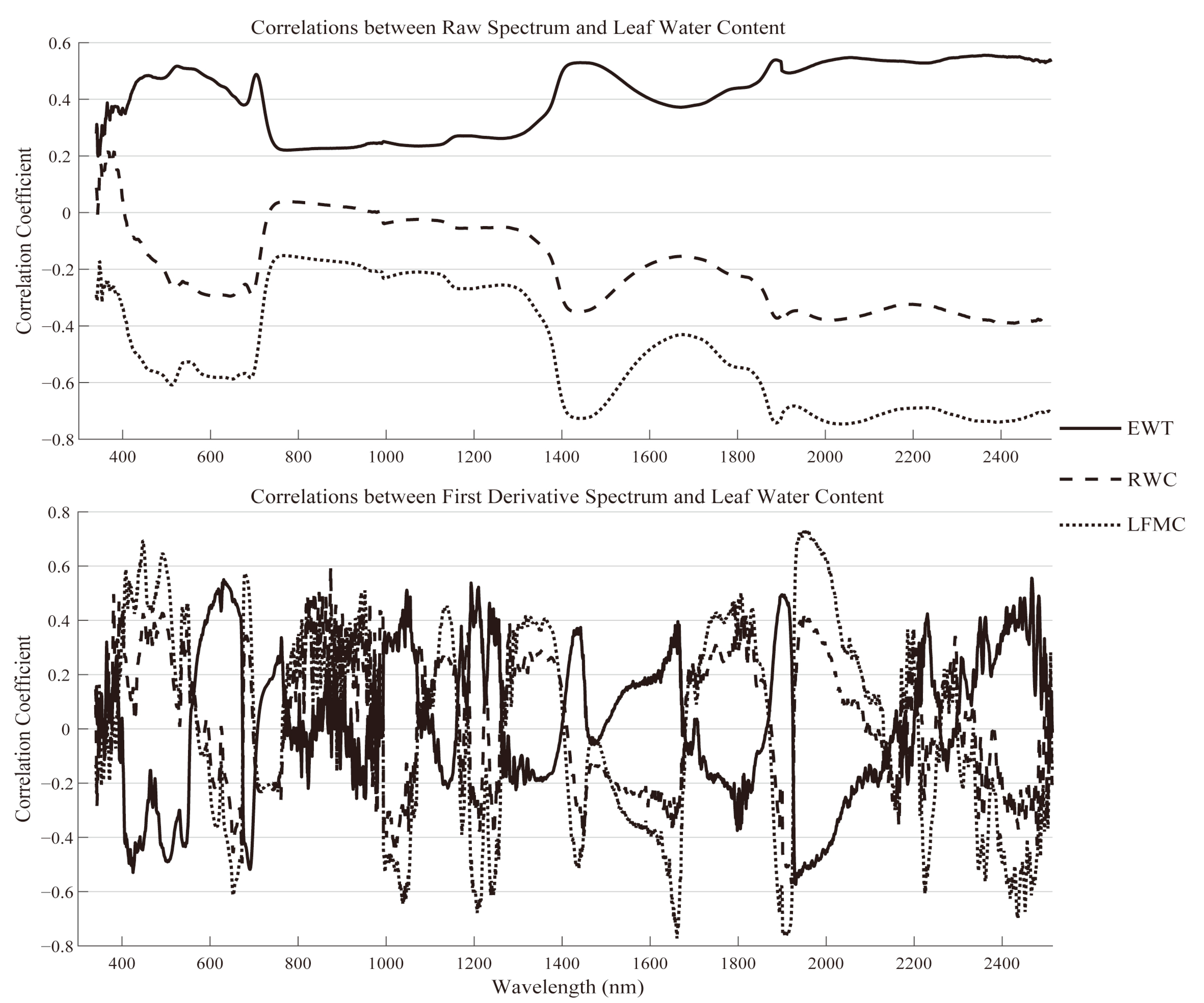
3.2.1. Correlations between Raw Spectrum, Derivative Spectrum, and Leaf Water Content Data

The Pearson correlation coefficient is one of the most commonly used indicators in correlation analysis [58] and was used in this paper. Correlation analysis of EWT, RWC, and LFMC was performed using raw leaf spectrum and first-derivative spectrum data from throughout the monitoring period (16 October–15 November; Figure 5). The results show that the raw spectra of leaves were positively correlated with EWT at all wavelengths, negatively correlated with RWC except at a small number of visible wavelengths (VIS, 400–780 nm), and negatively correlated with LFMC at all wavelengths. Overall, the EWT, RWC, and raw spectrum correlations were weak ( | r | < 0.6 ), of which the RWC was weaker, while LFMC was best in the short-wave infrared band (SWIR, 1400–2500 nm) to obtain the strong correlation band ( | r | > 0.7 ), and the correlation was strongest at 1889 nm ( r = 0.75 ). The first-derivative spectrum can effectively suppress influences such as the soil background. In the correlation analysis of the first-derivative spectrum, EWT and RWC, the positive and negative correlations were uncertain, and the absolute values of the correlation coefficients were small. The performance of LFMC continued to be excellent, with the maximum correlation coefficient between LFMC and the first-derivative spectrum appearing at 1661 nm ( r = 0.77 ).

3.2.2. Correlation between Spectral Reflectance Indices and Leaf Water Content

In remote sensing monitoring of plant water content, spectral reflectance indices have been widely used and are some of the most important spectral parameters. Therefore, we first analyzed the correlations between eight classical spectral reflectance indices and EWT, RWC, and LFMC (Table 2). The correlations between each index and EWT and RWC were weak. In contrast, the correlations between LFMC and each index were better. The spectral reflectance indices with good correlations with LFMC comprised bands mainly concentrated in the near-infrared and SWIR regions. The WI (1300,1450), NDVI, and NDII had correlations with LFMC of >0.6, among which the correlation between WI (1300,1450) and LFMC was the highest at 0.7. The results in Table 2 show that these classical spectral reflectance indices are not quite adequate for application in this paper, and a spectral reflectance index with better correlation needs to be constructed.
To find the best spectral reflectance indices for estimating leaf water content, the correlations between the ratio (RVI), normalized difference (NDVI), and difference (DVI) vegetation indices of the two bands in the 340–2500 nm range with EWT, RWC, and LFMC were systematically analyzed. Figure 6 presents a matrix of the correlation coefficients based on the different band combinations of the raw full-band spectrum and the leaf water content. The results show that the correlations between the vegetation indices and EWT and RWC were still weak, with LFMC performing best, which is consistent with the previous analysis. From Figure 6g–i, the three indices with the highest correlation coefficients r (RVI (1525,1771), DVI (1412,740), and NDVI (1447,1803)) were screened out, with the r-values being 0.81, 0.82, and 0.77, respectively. The band compositions of the three vegetation indices are in the near-infrared and SWIR, and they were highly correlated with the LFMC. Therefore, they can be preliminarily used as the spectral characteristic parameters of the LFMC.

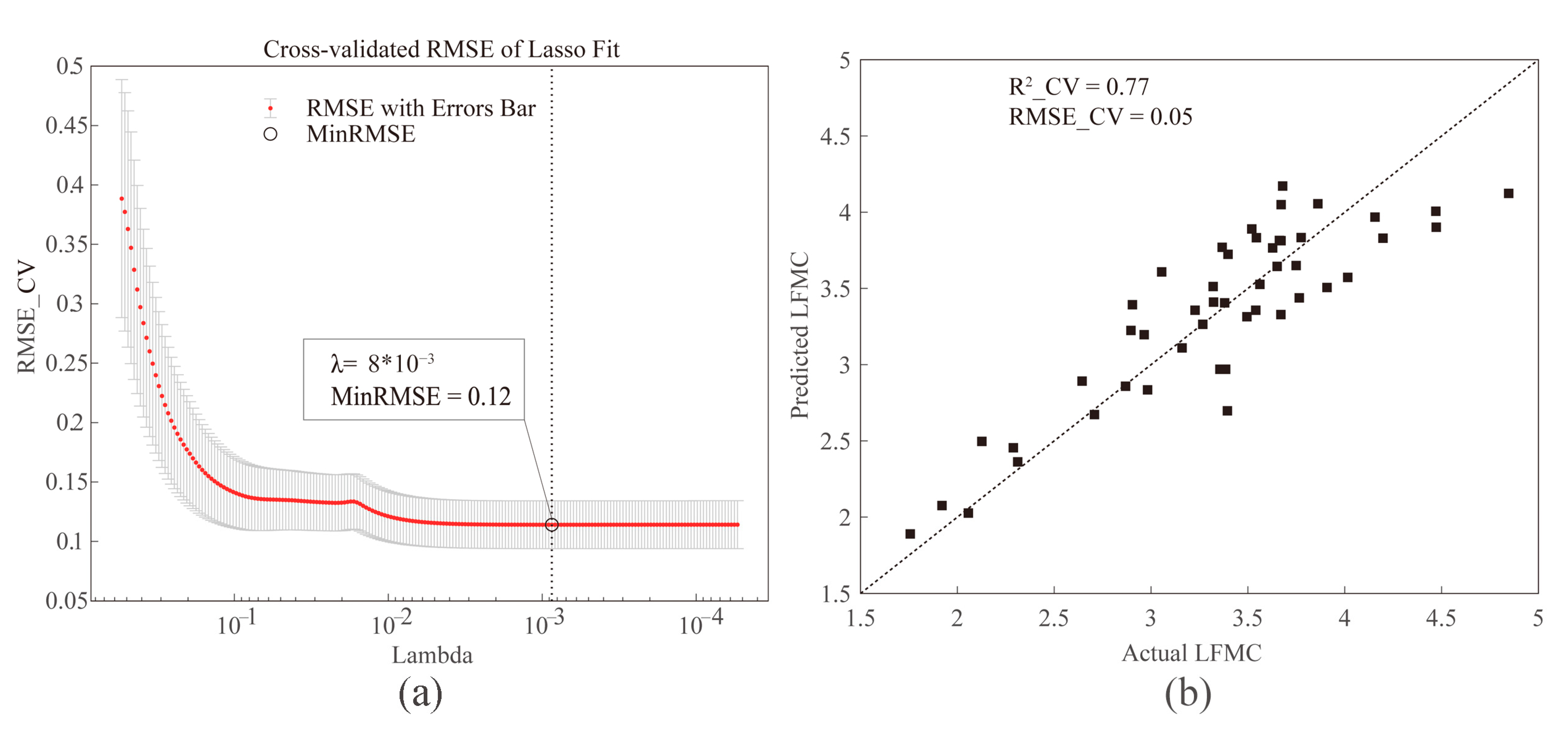
3.3. Optimal Spectral Features

According to the temporal changes in leaf water content and the correlation analysis with the raw spectral data, first-derivative spectrum, and spectral reflectance index, it is obvious that LFMC is the best water indicator for assessing heat stress, while EWT and RWC are not suitable. Based on correlation analysis, RS (1889; raw spectral value at 1889 nm), FDS (1661; first-derivative spectral value at 1661 nm), RVI (1525,1771), DVI (1412,740), and NDVI (1447,1803) were the five spectral features with strong correlations with LFMC. In general, selecting more features is not necessarily better, and data redundancy will reduce computational efficiency and affect the accuracy and applicability of the model. Therefore, it is necessary to further screen the spectral characteristic parameters of LFMC.
The regular term constructed in the Lasso regression model makes it possible to compress the dimension of the input sample. First, we need to determine the optimal regular coefficient Lambda (λ) and adopt 10-fold cross-validation for the dataset (Figure 7a). As shown in Figure 7a, the minimum λ of the RMSE was obtained after multiple iterations and was used as the regular term coefficient of the model. Then, the compressed spectral characteristic parameters were determined, and the accuracy of the regression model was tested. The results are shown in Table 3 and Figure 7b. It can be seen from Table 3 that RS (1889), as an independent variable, is compressed to 0 in the model, indicating that RS (1889) is removed from the input dimension. The R2-value of the Lasso regression model constructed with FDS (1661), RVI (1525,1771), DVI (1412,740), and NDVI (1447,1803) as independent variables was 0.77 with an RMSE of 0.05. Although the spectral features were reduced, the model accuracy was still high.

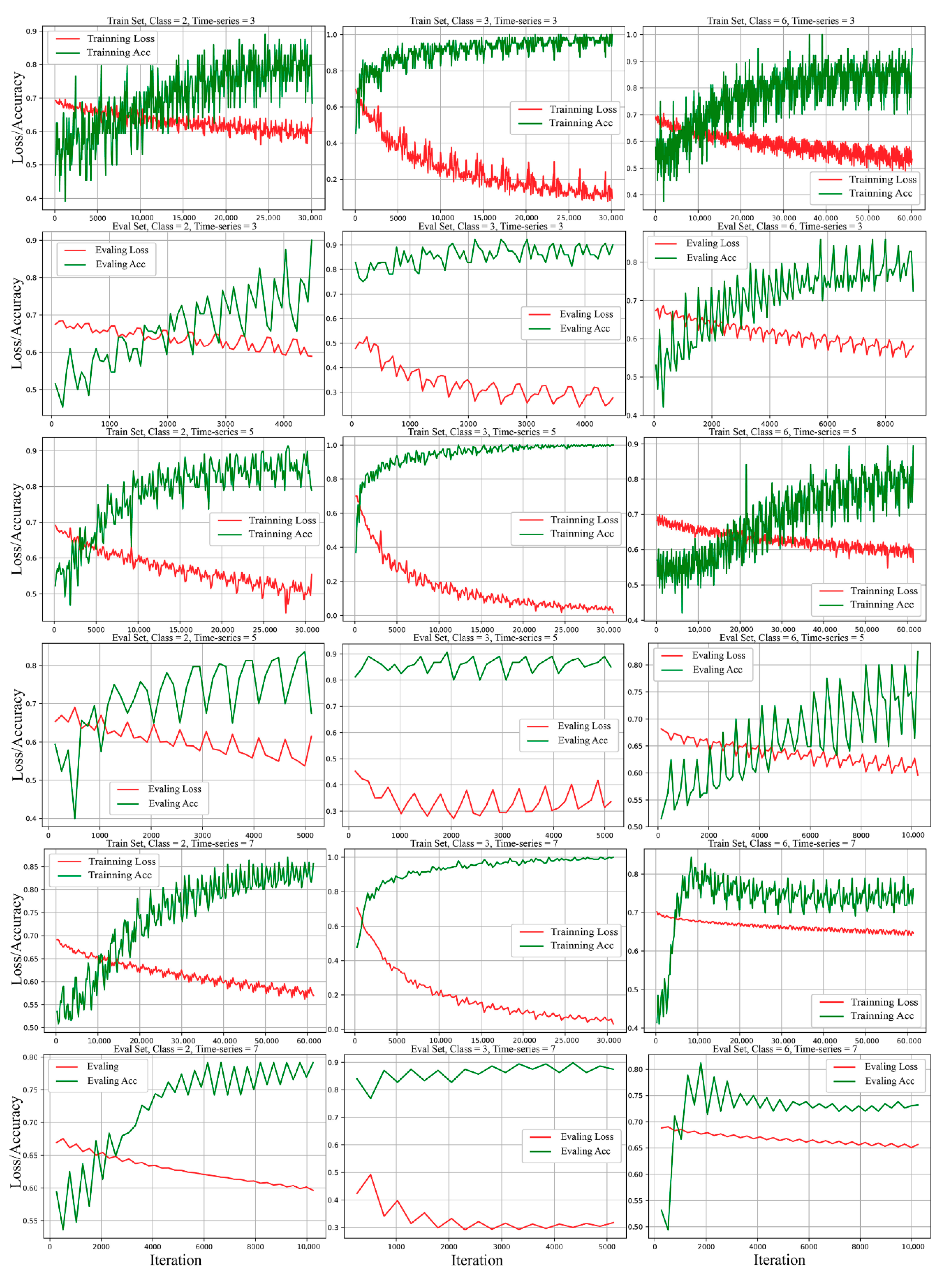
3.4. SF-LSTM Estimation of Heat-Stress Level

The direct use of spectral characteristics to accurately estimate the stress level in plants requires full consideration of the temporal changes in spectral data under different stress levels. Although it is sometimes feasible to estimate the spectral data in a single period, its generalization ability is often weak. To solve this problem, the spectral features of the time series were used as input to construct an SF-LSTM, and the estimation of plant stress level was transformed into a classification problem. The network structure is shown in Figure 4. To find the optimal model, the input layer data were set up with unified spectral features and different time series lengths, and different classification strategies were trialed: (1) spectral features: FDS(1661), RVI(1525,1771), DVI(1412,740), and NDVI(1447,1803); (2) time series: the time series length of spectral features was divided into lengths of 3, 5, and 7 (each length is a continuous date and does not reverse repeat); (3) classification strategies: two categories (control group and experimental groups), three categories (control group, T1 and T2, and T3, T4, and T5) and six categories (control group and each of the five experimental groups). The number of samples in each test was determined by the length of the time series, and the ratio of the training set to the verification set was 4:1. The number of output layer categories was consistent with the number of stress level categories. The initial learning rate was 0.01, and the batch size was adjusted according to the sample size. The adaptive moment estimate (Adam) was selected by the network optimizer and the cross-entropy error function was adopted as the loss function. The classification results are shown in Figure 8.
When using deep learning to estimate the heat-stress level in terms of a binary classification or multiple classification problem, the classification of categories has a huge impact on the modeling results. The test results show that the classification strategy determines the convergence of the model’s loss and accuracy and the overall stability of the model. Under the same classification strategy, the time series length of spectral features determines the level of model accuracy. As shown in Figure 8, among the different classification strategies, the loss and accuracy of the dichotomy model converged, the accuracies of the training set and evaluation set were not ideal, and the stability of the model was low. When divided into six categories, the model cannot converge many times and its stability is very poor. The heat-stress level was divided into three categories. The model training set had the highest accuracy, and the accuracy convergence value was >95%. Under different time series lengths, the effect was not good at a time series length of three. When the time series length of the data was five, the training set loss and accuracy had good convergence. The evaluation set had high accuracy and good stability, and its accuracy was stable at about 90%. Overfitting occurred at a time series length of seven. The overall results show that the SF-LSTM model is suitable for estimating heat stress when the classification strategies are divided into three categories, and the time series length is five.

4. Discussion

In this study, alfalfa was used to simulate thermal stress in a coal gangue dump reclamation area to conduct a gradient test with several treatments (control group, T1 = 60 °C, T2 = 90 °C, T3 = 120 °C, T4 = 150 °C, T5 = 180 °C). Water content and hyperspectral data on alfalfa leaves were collected one month before the flowering period. Correlation analysis and selection of the spectral features of alfalfa leaf water content were carried out. Based on the SF-LSTM model, the stress level in alfalfa under heat stress was estimated.

4.1. Leaf Water Content

The LFMC showed obvious regularity under different temperature gradients, which may be due to the calculations of LFMC and leaf dry and fresh weights. Root system growth has a huge impact on the dry and fresh weights of the plant leaves. As the heat-stress time increases, the supply of water and nutrients to plant leaves becomes insufficient. Long-term high soil temperatures cause significant changes in the LFMC of plant leaves. Compared with high air temperature, the photochemical efficiency of leaves and the root growth of plants are more severely affected by stress due to high soil temperature. Ref. [59] also reported that shoot growth and senescence in winter wheat are influenced more by soil temperature than air temperature. The adverse effects of high soil temperature on physiological activities are probably due to direct inhibition of root growth and activity and, therefore, limitation of water and nutrient supplies to the leaves [60] and disruption of cytokinin synthesis in roots [61]. High soil temperatures also promote leaf senescence by increasing the transport of root abscisic acid (ABA) to the leaves [62]. Although there were fluctuations in EWT and RWC during the monitoring period, the regularity was weak. This may be due to water shortages in the plant leaves, lack of nutrients, and destruction of the internal microstructure of the leaves under different degrees of high soil temperatures [63], resulting in varying degrees of change in leaf area and saturated water content.

4.2. Spectral Features

Changes in leaf spectra are usually affected by changes in chlorophyll, water content, internal structure, dry matter content, etc. The reflectance spectra of green plants in the 1000–2500 nm region are mainly influenced by liquid water and dry compounds. The water absorption band is 1360–2080 nm, which is highly correlated with leaf water content and is not affected by leaf structure [64]. This study shows that the band sensitive to the leaf water content of alfalfa under high soil temperature heat stress is mainly concentrated in the long-wave infrared region (1400–2500 nm). Correlation analysis of the raw and first-derivative spectra with water content data showed that the bands at 1889 nm and 1661 nm had the highest correlations with LFMC, which was the optimal spectral feature (see Figure 3). This is similar to previous studies [65].
Due to the strong reflection from the surfaces of fresh leaves and the influences of the surface and internal structures of leaf cuticles, leaf hairs, etc., it is difficult to comprehensively and accurately estimate plant moisture status using a single band of spectral reflectance. By constructing a vegetation index, the effective spectral information of the vegetation can be maximized, the single-band scattering effect can be effectively reduced, and prediction accuracy can be improved [66]. This article analyzed the correlations between the ratio, difference, and normalized vegetation indexes and leaf water content in any two bands within 340–2500 nm. It found that the correlations between various indexes and LFMC were all high. Specifically, the three spectral features RVI (1525,1771), DVI (1412,740), and NDVI (1447,1803) had the highest correlations. The results of this part of the correlation analysis also verify that LFMC is the most suitable water content indicator for this study on temporal changes in leaf water content.
Through correlation analysis, we screened out several spectral features with strong correlations with LFMC. However, in multiple regression, when the independent variable has a higher dimension, there are often problems such as collinearity and data redundancy [67]. Using the Lasso regression model to further optimize the above-mentioned spectral features can minimize the adverse effects of multi-dimensional input data on the assessment results when estimating the heat-stress level. After dimensionality reduction and Lasso regression, the spectral features selected in this paper were FDS (1661), RVI (1525,1771), DVI (1412,740), and NDVI (1447,1803).

4.3. Heat Stress Estimation

Considering the importance of temporal sequences in the estimation of plant environmental stress, LSTM (which can effectively utilize a temporal sequence of data in deep learning) was used to build an heat-stress model. Meanwhile, stress-level estimates were presented in the form of classification results for the application scenarios considered in this paper. Compared with traditional machine learning classification methods, LSTM is more effective in classifying remote sensing time series data [68]. A variety of classification strategies and time-series-length models were tested. The dichotomy strategy was the most common strategy used in the classification model. According to the results in Figure 8, although the parameters of the model constructed using the dichotomy strategy can converge, the accuracy was not acceptable. This may be related to the large difference in the proportion of the number of samples of the two categories in the training set and the evaluation set. In the next step of the study, this adverse factor was reduced by increasing the sample size of the control group during experimental data collection. Among the multi-classification strategies, three categories had the best effects. The longer the time series, the better. The model had the highest accuracy with a sequence length of five. This conclusion is in line with the laws of deep learning. Over-redundant data, complex neural network architectures, and inappropriate classification strategies not only make models unable to fit the data, but also lead to over-fitting [69]. Over-fitted models have poor generalization ability and weak applicability.

5. Conclusions

In this study, an SF-LSTM model was established by using the time series spectral features of leaf water content obtained through an experiment that simulated heat stress in coal gangue dump reclamation areas. The model was effective in estimating the heat-stress level in alfalfa. Through time series analysis of leaf water content data, it was found that the EWT and RWC do not have high regularity over time, making it difficult to distinguish between normal and heat damage statuses in alfalfa. Heat stress in alfalfa was best indicated by the LFMC leaf water content index. According to correlation analysis of the raw spectrum, first-derivative spectrum, three forms of vegetation index, and leaf water content data, RS(1889), FDS(1661), RVI(1525,1771), DVI(1412,740), and NDVI(1447,1803) had the strongest correlations with LFMC. After further screening by the Lasso regression model, FDS(1661), RVI(1525,1771), DVI(1412,740), and NDVI(1447,1803) were found to be the optimal spectral features of inversion LFMC and can be used as spectral features to assess heat stress. The SF-LSTM model was constructed to estimate the heat-stress level in alfalfa based on a time series of spectral features. The results show that this model can estimate the stress level with high accuracy when the classification strategies are divided into three categories (control group, T1 and T2, and T3, T4, and T5) and a spectral feature time series length of five (where the dates in the monitoring period are continuous without repetition). The results of this study provide a new way to assess plant heat stress in coal gangue dump reclamation areas. This has important practical application value and is expected to be further verified and applied in other types of environmental stress research. Subsequent studies will verify the conclusions of this experiment at larger spatial scales.

Supplementary Materials

The following are available online at https://0-www-mdpi-com.brum.beds.ac.uk/article/10.3390/rs13132634/s1, Figure S1: Mean and Gaussian filtered spectra of alfalfa leaves.

Author Contributions

Q.W. and F.Y.: conceptualization, methodology, data curation: application of statistical, mathematical, computational, or other formal techniques to analyze or synthesize study data, visualization, writing—original draft preparation. Y.Z. and W.X.: writing—review and editing, funding acquisition, conceptualization. T.L. and H.S.: provision of study materials, laboratory samples, instrumentation. All authors have read and agreed to the published version of the manuscript.

Funding

This research was funded by the National Key Research and Development Program of China, grant number 2016YF C0501103-4 and 2016YF C0501103-5.

Institutional Review Board Statement

Not applicable.

Informed Consent Statement

Not applicable.

Data Availability Statement

The data presented in this study are available on request from the corresponding author. The data are not publicly available due to the follow-up related work has not been completed.

Acknowledgments

This work was supported by the National Key Research and Development Program of China [grant numbers 2016YF C0501103-4, 2016YF C0501103-5]. The authors wish to express heartfelt thanks to Yang Tianle, Yao Zhaosheng, Zhang Weijun, and Lin Zihan for data acquisition work and to Wang Dunliang and Li Rui for debugging the test equipment.

Conflicts of Interest

The authors declare no conflict of interest.

References

  1. Onifade, M.; Genc, B. Spontaneous combustion liability of coal and coal-shale: A review of prediction methods. Int. J. Coal Sci. Technol. 2019, 6, 151–168. [Google Scholar] [CrossRef] [Green Version]
  2. Alekseenko, V.A.; Bech, J.; Alekseenko, A.V.; Shvydkaya, N.V.; Roca, N. Environmental impact of disposal of coal mining wastes on soils and plants in Rostov Oblast, Russia. J. Geochem. Explor. 2018, 184, 261–270. [Google Scholar] [CrossRef]
  3. Wu, Y.; Yu, X.; Hu, S.; Shao, H.; Liao, Q.; Fan, Y. Experimental study of the effects of stacking modes on the spontaneous combustion of coal gangue. Process Saf. Environ. 2019, 123, 39–47. [Google Scholar] [CrossRef]
  4. Li, J.; Wang, J. Comprehensive utilization and environmental risks of coal gangue: A review. J. Clean. Prod. 2019, 239, 117946. [Google Scholar] [CrossRef]
  5. Nie, X.; Zhao, T.; Su, Y. Fossil fuel carbon contamination impacts soil organic carbon estimation in cropland. Catena 2021, 196, 104889. [Google Scholar] [CrossRef]
  6. Wang, H.; Tan, B.; Zhang, X. Research on the technology of detection and risk assessment of fire areas in gangue hills. Environ. Sci. Pollut. R. 2020, 27, 38776–38787. [Google Scholar] [CrossRef] [PubMed]
  7. Xing, Y.; Feng, J.; Rong, X. Discussion on causes of combustion and explosion and of coal gangue at the No. 4 mine of Pingdingshan coal Mine and countermeasures. Chin. J. Geol. Hazard. Control 2007, 18, 145–150. [Google Scholar]
  8. Sloss, L.L. Assessing and Managing Spontaneous Combustion of Coal; IEA Clean Coal Centre: Washington, DC, USA, 2015. [Google Scholar]
  9. Querol, X.; Zhuang, X.; Font, O.; Izquierdo, M.; Alastuey, A.; Castro, I.; Van Drooge, B.L.; Moreno, T.; Grimalt, J.O.; Elvira, J. Influence of soil cover on reducing the environmental impact of spontaneous coal combustion in coal waste gobs: A review and new experimental data. Int. J. Coal Geol. 2011, 85, 2–22. [Google Scholar] [CrossRef]
  10. Xiaoshuai, W.; Yuegang, T.; Wang, S.; Schobert, H.H. Clean coal geology in China: Research advance and its future. Int. J. Coal Sci. Technol. 2020, 7, 299–310. [Google Scholar]
  11. Roy, P.; Guha, A.; Kumar, K.V. An approach of surface coal fire detection from ASTER and Landsat-8 thermal data: Jharia coal field, India. Int. J. Appl. Earth Obs. 2015, 39, 120–127. [Google Scholar] [CrossRef]
  12. Hu, Z.; Xia, Q. An integrated methodology for monitoring spontaneous combustion of coal waste dumps based on surface temperature detection. Appl. Therm. Eng. 2017, 122, 27–38. [Google Scholar] [CrossRef]
  13. Pandey, J.; Kumar, D.; Mishra, R.K.; Mohalik, N.K.; Khalkho, A.; Singh, V.K. Application of thermography technique for assessment and monitoring of coal mine fire: A special reference to Jharia Coal Field, Jharkhand, India. Int. J. Adv. Remote Sens. GIS 2013, 2, 138–147. [Google Scholar]
  14. Mishra, R.K.; Pandey, J.K.; Pandey, J.; Kumar, S.; Roy, P.N.S. Detection and analysis of coal fire in Jharia Coalfield (JCF) using Landsat remote sensing data. J. Indian Soc. Remote 2020, 48, 181–195. [Google Scholar] [CrossRef]
  15. Mishra, R.K.; Roy, P.; Singh, V.K.; Pandey, J.K. Detection and delineation of coal mine fire in Jharia coal field, India using geophysical approach: A case study. J. Earth Syst. Sci. 2018, 127, 1–10. [Google Scholar] [CrossRef] [Green Version]
  16. Misz-Kennan, M.; Tabor, A. The thermal history of selected coal waste dumps in the Upper Silesian Coal Basin (Poland). Coal Peat Fires A Glob. Perspect. 2011, 3, 431–474. [Google Scholar]
  17. Nádudvari, A.; Abramowicz, A.; Fabiańska, M.; Misz-Kennan, M.; Ciesielczuk, J. Classification of fires in coal waste dumps based on Landsat, Aster thermal bands and thermal camera in Polish and Ukrainian mining regions. Int. J. Coal Sci. Technol. 2020. [Google Scholar] [CrossRef]
  18. Rossi, S.; Burgess, P.; Jespersen, D.; Huang, B. Heat-induced leaf senescence associated with chlorophyll metabolism in Bentgrass lines differing in heat tolerance. Crop Sci. 2017, 57, 169–178. [Google Scholar] [CrossRef]
  19. Iqbal, N.; Umar, S.; Khan, N.A.; Corpas, F.J. Crosstalk between abscisic acid and nitric oxide under heat stress: Exploring new vantage points. Plant Cell Rep. 2021, 1–22. [Google Scholar] [CrossRef]
  20. Zhang, F.; Zhou, G. Estimation of canopy water content by means of hyperspectral indices based on drought stress gradient experiments of maize in the north plain China. Remote Sens. 2015, 7, 15203–15223. [Google Scholar] [CrossRef] [Green Version]
  21. Liu, W.; Huang, J.; Wei, C.; Wang, X.; Mansaray, L.R.; Han, J.; Zhang, D.; Chen, Y. Mapping water-logging damage on winter wheat at parcel level using high spatial resolution satellite data. ISPRS J. Photogramm. Remote. Sens. 2018, 142, 243–256. [Google Scholar] [CrossRef]
  22. Song, Y.; Wu, C. Examining human heat stress with remote sensing technology. Gisci. Remote Sens. 2018, 55, 19–37. [Google Scholar] [CrossRef]
  23. Ma, B.; Pu, R.; Zhang, S.; Wu, L. Spectral identification of stress types for maize seedlings under single and combined stresses. IEEE Access 2018, 6, 13773–13782. [Google Scholar] [CrossRef]
  24. Zhou, X.; Sun, J.; Tian, Y.; Lu, B.; Hang, Y.; Chen, Q. Development of deep learning method for lead content prediction of lettuce leaf using hyperspectral images. Int. J. Remote Sens. 2020, 41, 2263–2276. [Google Scholar] [CrossRef]
  25. Caballero, D.; Calvini, R.; Amigo, J.M. Hyperspectral imaging in crop fields: Precision agriculture. In Data Handling in Science and Technology; Elsevier: Amsterdam, The Netherlands, 2020; Volume 32, pp. 453–473. [Google Scholar]
  26. Cao, Z.; Wang, Q.; Zheng, C. Best hyperspectral indices for tracing leaf water status as determined from leaf dehydration experiments. Ecol. Indic. 2015, 54, 96–107. [Google Scholar] [CrossRef]
  27. Nigam, R.; Vyas, S.S.; Bhattacharya, B.K.; Oza, M.P.; Manjunath, K.R. Retrieval of regional LAI over agricultural land from an Indian geostationary satellite and its application for crop yield estimation. J. Spat. Sci. 2017, 62, 103–125. [Google Scholar] [CrossRef]
  28. Kong, W.; Huang, W.; Liu, J.; Chen, P.; Qin, Q.; Ye, H.; Peng, D.; Dong, Y.; Mortimer, A.H. Estimation of canopy carotenoid content of winter wheat using multi-angle hyperspectral data. Adv. Space Res. 2017, 60, 1988–2000. [Google Scholar] [CrossRef]
  29. Sperdouli, I.; Moustakas, M. Spatio-temporal heterogeneity in Arabidopsis thaliana leaves under drought stress. Plant Biol. 2012, 14, 118–128. [Google Scholar] [CrossRef]
  30. Zhang, F.; Zhou, G. Estimation of vegetation water content using hyperspectral vegetation indices: A comparison of crop water indicators in response to water stress treatments for summer maize. BMC Ecol. 2019, 19, 18. [Google Scholar] [CrossRef] [Green Version]
  31. Liu, C.; Sun, P.; Liu, S. A review of plant spectral reflectance response to water physiological changes. Chin. J. Plant Ecol. 2016, 40, 80. [Google Scholar]
  32. Yebra, M.; Dennison, P.E.; Chuvieco, E.; Riano, D.; Zylstra, P.; Hunt Jr, E.R.; Danson, F.M.; Qi, Y.; Jurdao, S. A global review of remote sensing of live fuel moisture content for fire danger assessment: Moving towards operational products. Remote Sens. Environ. 2013, 136, 455–468. [Google Scholar] [CrossRef]
  33. Peñuelas, J.; Filella, I.; Biel, C.; Serrano, L.; Save, R. The reflectance at the 950–970 nm region as an indicator of plant water status. Int. J. Remote Sens. 1993, 14, 1887–1905. [Google Scholar] [CrossRef]
  34. Berger, K.; Atzberger, C.; Danner, M.; Urso, G.D.; Mauser, W.; Vuolo, F.; Hank, T. Evaluation of the PROSAIL model capabilities for future hyperspectral model environments: A review study. Remote Sens. 2018, 10, 85. [Google Scholar] [CrossRef] [Green Version]
  35. Boren, E.J.; Boschetti, L. Landsat-8 and Sentinel-2 Canopy Water Content Estimation in Croplands through Radiative Transfer Model Inversion. Remote Sens. 2020, 12, 2803. [Google Scholar] [CrossRef]
  36. Rodríguez-Pérez, J.R.; Ordó Ez, C.; González-Fernández, A.B.; Sanz-Ablanedo, E.; Valenciano, J.B.; Marcelo, V. Leaf water content estimation by functional linear regression of field spectroscopy data. Biosyst. Eng. 2018, 165, 36–46. [Google Scholar] [CrossRef]
  37. Ge, Y.; Bai, G.; Stoerger, V.; Schnable, J.C. Temporal dynamics of maize plant growth, water use, and leaf water content using automated high throughput RGB and hyperspectral imaging. Comput. Electron. Agric. 2016, 127, 625–632. [Google Scholar] [CrossRef] [Green Version]
  38. Virnodkar, S.S.; Pachghare, V.K.; Patil, V.C.; Jha, S.K. Remote sensing and machine learning for crop water stress determination in various crops: A critical review. Precis. Agric. 2020, 21, 1121–1155. [Google Scholar] [CrossRef]
  39. Yebra, M.; Quan, X.; Riaño, D.; Larraondo, P.R.; van Dijk, A.I.; Cary, G.J. A fuel moisture content and flammability monitoring methodology for continental Australia based on optical remote sensing. Remote Sens. Environ. 2018, 212, 260–272. [Google Scholar] [CrossRef]
  40. Yi, Q.; Bao, A.; Wang, Q.; Zhao, J. Estimation of leaf water content in cotton by means of hyperspectral indices. Comput. Electron. Agric. 2013, 90, 144–151. [Google Scholar] [CrossRef]
  41. Krishna, G.; Sahoo, R.N.; Singh, P.; Bajpai, V.; Patra, H.; Kumar, S.; Dandapani, R.; Gupta, V.K.; Viswanathan, C.; Ahmad, T. Comparison of various modelling approaches for water deficit stress monitoring in rice crop through hyperspectral remote sensing. Agric. Water Manag. 2019, 213, 231–244. [Google Scholar] [CrossRef]
  42. Xiong, X.; Liu, N.; Wei, Y.; Bi, Y.; Luo, J.; Xu, R.; Zhou, J.; Zhang, Y. Effects of non-uniform root zone salinity on growth, ion regulation, and antioxidant defense system in two alfalfa cultivars. Plant Physiol. Biochem. 2018, 132, 434–444. [Google Scholar] [CrossRef] [PubMed]
  43. Wang, J.; Li, X.; Bai, Z.; Huang, L. The effects of coal gangue and fly ash on the hydraulic properties and water content distribution in reconstructed soil profiles of coal-mined land with a high groundwater table. Hydrol. Process 2017, 31, 687–697. [Google Scholar] [CrossRef]
  44. Thorp, K.R.; Wang, G.; Bronson, K.F.; Badaruddin, M.; Mon, J. Hyperspectral data mining to identify relevant canopy spectral features for estimating durum wheat growth, nitrogen status, and grain yield. Comput. Electron. Agric. 2017, 136, 1–12. [Google Scholar] [CrossRef] [Green Version]
  45. Atzberger, C.; Darvishzadeh, R.; Immitzer, M.; Schlerf, M.; Skidmore, A.; Maire, G.L. Comparative analysis of different retrieval methods for mapping grassland leaf area index using airborne imaging spectroscopy. Int. J. Appl. Earth Obs. Geoinf. 2015, 43, 19–31. [Google Scholar] [CrossRef] [Green Version]
  46. Caturegli, L.; Matteoli, S.; Gaetani, M.; Grossi, N.; Magni, S.; Minelli, A.; Corsini, G.; Remorini, D.; Volterrani, M. Effects of water stress on spectral reflectance of bermudagrass. Sci. Rep. 2020, 10, 1–12. [Google Scholar] [CrossRef]
  47. Seelig, H.D.; Hoehn, A.; Stodieck, L.S.; Klaus, D.M.; Adams, W.W.; Emery, W.J. Plant water parameters and the remote sensing R 1300/R 1450 leaf water index: Controlled condition dynamics during the development of water deficit stress. Irrig. Sci. 2009, 27, 357–365. [Google Scholar] [CrossRef]
  48. Ihuoma, S.O.; Madramootoo, C.A. Recent advances in crop water stress detection. Comput. Electron. Agric. 2017, 141, 267–275. [Google Scholar] [CrossRef]
  49. Wolf, A.F. Using WorldView-2 Vis-NIR multispectral imagery to support land mapping and feature extraction using normalized difference index ratios. In Algorithms and Technologies for Multispectral, Hyperspectral and Ultraspectral Imagery XVIII; International Society for Optics and Photonics: Baltimore, MD, USA, 2012; Volume 8390. [Google Scholar]
  50. Maimaitiyiming, M.; Ghulam, A.; Bozzolo, A.; Wilkins, J.L.; Kwasniewski, M.T. Early detection of plant physiological responses to different levels of water stress using reflectance spectroscopy. Remote Sens. 2017, 9, 745. [Google Scholar] [CrossRef] [Green Version]
  51. Joiner, J.; Yoshida, Y.; Anderson, M.; Holmes, T.; Hain, C.; Reichle, R.; Koster, R.; Middleton, E.; Zeng, F. Global relationships among traditional reflectance vegetation indices (NDVI and NDII), evapotranspiration (ET), and soil moisture variability on weekly timescales. Remote Sens. Environ. 2018, 219, 339–352. [Google Scholar] [CrossRef] [PubMed] [Green Version]
  52. Peng, D.; Zhang, H.; Yu, L.; Wu, M.; Wang, F.; Huang, W.; Liu, L.; Sun, R.; Li, C.; Wang, D. Assessing spectral indices to estimate the fraction of photosynthetically active radiation absorbed by the vegetation canopy. Int. J. Remote Sens. 2018, 39, 8022–8040. [Google Scholar] [CrossRef]
  53. Sukhova, E.; Sukhov, V. Connection of the photochemical reflectance index (PRI) with the photosystem II quantum yield and nonphotochemical quenching can be dependent on variations of photosynthetic parameters among investigated plants: A meta-analysis. Remote Sens. 2018, 10, 771. [Google Scholar] [CrossRef] [Green Version]
  54. Tibshirani, R. Regression shrinkage and selection via the lasso. J. R. Stat. Soc. Ser. B 1996, 58, 267–288. [Google Scholar] [CrossRef]
  55. Hochreiter, S.; Schmidhuber, J. Long short-term memory. Neural Comput. 1997, 9, 1735–1780. [Google Scholar] [CrossRef] [PubMed]
  56. Kim, J. Estimating classification error rate: Repeated cross-validation, repeated hold-out and bootstrap. Comput. Stat. Data Anal. 2009, 53, 3735–3745. [Google Scholar] [CrossRef]
  57. Anderson, S.A.; Anderson, W.R. Ignition and fire spread thresholds in gorse (Ulex europaeus). Int. J. Wildland Fire 2010, 19, 589–598. [Google Scholar] [CrossRef]
  58. Zhang, W.; Li, X.; Zhao, L. A fast hyperspectral feature selection method based on band correlation analysis. IEEE Geosci. Remote Sens. Lett. 2018, 15, 1750–1754. [Google Scholar] [CrossRef]
  59. Pramanik, P.; Chakrabarti, B.; Bhatia, A.; Singh, S.D.; Maity, A.; Aggarwal, P.; Krishnan, P. Effect of elevated temperature on soil hydrothermal regimes and growth of wheat crop. Environ. Monit. Assess. 2018, 190, 1–10. [Google Scholar] [CrossRef] [PubMed]
  60. Khalil, U.; Ali, S.; Rizwan, M.; Rahman, K.U.; Ata-Ul-Karim, S.T.; Najeeb, U.; Ahmad, M.N.; Adrees, M.; Sarwar, M.; Hussain, S.M. Role of mineral nutrients in plant growth under extreme temperatures. In Plant Nutrients and Abiotic Stress Tolerance; Springer: Berlin/Heidelberg, Germany, 2018; pp. 499–524. [Google Scholar]
  61. Smart, C.M.; Scofield, S.R.; Bevan, M.W.; Dyer, T.A. Delayed leaf senescence in tobacco plants transformed with tmr, a gene for cytokinin production in Agrobacterium. Plant Cell 1991, 3, 647–656. [Google Scholar] [CrossRef]
  62. Liu, X.; Huang, B. Root physiological factors involved in cool-season grass response to high soil temperature. Environ. Exp. Bot. 2005, 53, 233–245. [Google Scholar] [CrossRef]
  63. Xu, Q.; Huang, B. Growth and physiological responses of creeping bentgrass to changes in air and soil temperatures. Crop Sci. 2000, 40, 1363–1368. [Google Scholar] [CrossRef]
  64. Zhang, L.; Zhou, Z.; Zhang, G.; Meng, Y.; Chen, B.; Wang, Y. Monitoring the leaf water content and specific leaf weight of cotton (Gossypium hirsutum L.) in saline soil using leaf spectral reflectance. Eur. J. Agron. 2012, 41, 103–117. [Google Scholar] [CrossRef]
  65. Wu, J.; Chen, T.S.; Pan, L.X. Spectrum Variance Analysis of Tree Leaves under the Condition of Different Leaf water Content. Guang Pu Xue Yu Guang Pu Fen Xi = Guang Pu 2015, 35, 1961–1966. [Google Scholar]
  66. Cheng, T.; Rivard, B.; Sanchez-Azofeifa, A. Spectroscopic determination of leaf water content using continuous wavelet analysis. Remote Sens. Environ. 2011, 115, 659–670. [Google Scholar] [CrossRef]
  67. Dormann, C.F.; Elith, J.; Bacher, S.; Buchmann, C.; Carl, G.; Carré, G.; Marquéz, J.R.G.; Gruber, B.; Lafourcade, B.; Leitao, P.J. Collinearity: A review of methods to deal with it and a simulation study evaluating their performance. Ecography 2013, 36, 27–46. [Google Scholar] [CrossRef]
  68. De Castro Filho, H.C.; De Carvalho Júnior, O.A.; De Carvalho, O.L.F.; De Bem, P.P.; Dos Santos De Moura, R.; De Albuquerque, A.O.; Rosa Silva, C.; Guimarães Ferreira, P.H.; Fontes Guimarães, R.; Trancoso Gomes, R.A. Rice crop detection using LSTM, Bi-LSTM, and machine learning models from Sentinel-1 time series. Remote Sens. 2020, 12, 2655. [Google Scholar] [CrossRef]
  69. Karim, F.; Majumdar, S.; Darabi, H.; Chen, S. LSTM fully convolutional networks for time series classification. IEEE Access 2017, 6, 1662–1669. [Google Scholar] [CrossRef]
Figure 1. (a) Field of simulation experiment of heat stress in alfalfa and (b) schematic diagram of the heating equipment.
Remotesensing 13 02634 g001
Figure 2. Schematic diagram of one-dimensional Gaussian filtering along the spectrum direction, with a sliding window of 5.
Remotesensing 13 02634 g002
Figure 3. SF-LSTM network structure diagram.
Remotesensing 13 02634 g003
Figure 4. Time series of equivalent water thickness (EWT), live fuel moisture content (LFMC), and relative water content (RWC) in the control and experimental groups at leaf level from 16 October–15 November 2020; letters a, b, c, d and e are labeled to show significant differences between treatments within each measurement date.
Remotesensing 13 02634 g004
Figure 5. Coefficients of correlation between EWT, RWC, LFMC, and the raw leaf and first-derivative spectral data.
Remotesensing 13 02634 g005
Figure 6. Coefficients of correlation between EWT, RWC, and LFMC with RVI (λ1, λ2), NDVI (λ1, λ2), DVI (λ1, λ2), and ratio/normalized difference/difference vegetation indexes constructed from raw spectral data. (a) Correlation between EWT and RVI (RVI band combinations based on raw reflectance relationship with EWT); (b) Correlation between EWT and DVI; (c) Correlation between EWT and NDVI; (d) Correlation between RWC and RVI; (e) Correlation between RWC and DVI; (f) Correlation between RWC and NDVI; (g) Correlation between LFMC and RVI; (h) Correlation between LFMC and DVI and (i) Correlation between LFMC and NDVI.
Remotesensing 13 02634 g006
Figure 7. (a) Use of 10-fold cross-validation to determine the regular coefficient (lambda, λ) of the Lasso model; (b) predicted and actual values of LFMC by Lasso regression.
Remotesensing 13 02634 g007
Figure 8. Loss and accuracy of the SF-LSTM model training set and validation set under different classification strategies and time series lengths.
Remotesensing 13 02634 g008
Table 1. Spectral reflectance indices related to leaf water content.
Water-SRIsAcronymEquation 1Reference
Water indexWI (900, 970) R 900 / R 970 [46]
Water indexWI (1300, 1450) R 1300 / R 1450 [47]
Normalized difference water indexNDWI ( R 870 R 1260 ) / ( R 870 + R 1260 ) [48]
Moisture stress indexMSI R 1610 / R 842 [49]
Vegetation-SRIsAcronymEquation 1Reference
Normalized difference vegetation indexNDVI ( R 858 R 645 ) / ( R 858 + R 645 ) [50]
Normalized difference infrared indexNDII ( R 858 R 645 ) / ( R 858 + R 645 ) [51]
Simple ratio vegetation indexSR R 800 / R 680 [52]
Photochemical reflectance indexPRI ( R 570 R 531 ) / ( R 570 + R 531 ) [53]
1  R λ = reflectance at wavelength λ .
Table 2. Coefficients of correlation (r) between existing spectral reflectance indices and leaf water content.
Water-SRIsrVegetation-SRIsr
EWTRWCLFMCEWTRWCLFMC
WI (900,970)0.34−0.39−0.64 *SR−0.37−0.33−0.57 *
WI (1300,1450)0.44−0.39−0.7 *NDVI0.39−0.33−0.57 *
NDWI0.22−0.57 *−0.59 *NDII0.33−0.44−0.63 *
MSI−0.350.420.64 *PRI−0.440.31−0.5
* Indicates significant differences at 95% confidence level.
Table 3. Correlation coefficients between existing vegetation indices and leaf water content.
Lasso RegressionRegression CoefficientsR2_CVRMSE_CV
Spectral Parameters
RS (1889)00.770.05
FDS (1661)29
RVI (1525,1771)30.93
DVI (1412,740)0.19
NDVI (1447,1803)−2.76
Equation 1 y = 29 x 1 + 30.93 x 2 + 0.19 x 3 2.76 x 4
1 y = LFMC; x 1 = FDS (1661);   x 2 = RVI (1525,1771);   x 3 = DVI (1412,740);   x 4 = NDVI (1447,1803).
Publisher’s Note: MDPI stays neutral with regard to jurisdictional claims in published maps and institutional affiliations.

