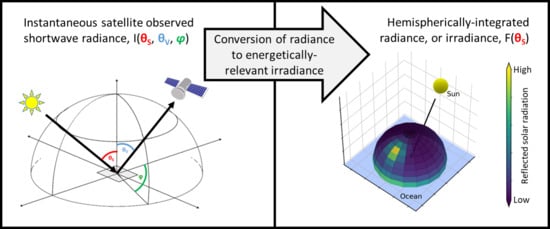
Shortwave Radiance to Irradiance Conversion for Earth Radiation Budget Satellite Observations: A Review

Abstract

Observing the Earth radiation budget (ERB) from satellites is crucial for monitoring and understanding Earth’s climate. One of the major challenges for ERB observations, particularly for reflected shortwave radiation, is the conversion of the measured radiance to the more energetically relevant quantity of radiative flux, or irradiance. This conversion depends on the solar-viewing geometry and the scene composition associated with each instantaneous observation. We first outline the theoretical basis for algorithms to convert shortwave radiance to irradiance, most commonly known as empirical angular distribution models (ADMs). We then review the progression from early ERB satellite observations that applied relatively simple ADMs, to current ERB satellite observations that apply highly sophisticated ADMs. A notable development is the dramatic increase in the number of scene types, made possible by both the extended observational record and the enhanced scene information now available from collocated imager information. Compared with their predecessors, current shortwave ADMs result in a more consistent average albedo as a function of viewing zenith angle and lead to more accurate instantaneous and mean regional irradiance estimates. One implication of the increased complexity is that the algorithms may not be directly applicable to observations with insufficient accompanying imager information, or for existing or new satellite instruments where detailed scene information is not available. Recent advances that complement and build on the base of current approaches, including machine learning applications and semi-physical calculations, are highlighted.

1. Introduction

Monitoring the amount of solar radiation (or shortwave radiation, in the spectral range from approximately 0.3 to 5 μm) reflected back to space by Earth is vital for understanding and modelling our climate system and its evolution [1,2]. The most comprehensive observations of reflected shortwave radiation to date have been obtained from dedicated Earth radiation budget (ERB) satellite instruments flown in low-Earth orbit [3,4,5,6,7,8]. Among these are relatively simple wide field-of-view (WFOV) non-scanning instruments that sample the entire Earth disk as a single pixel, and narrow field-of-view (NFOV) instruments that sample only a small area but provide coverage by scanning. The WFOV instruments present unique challenges for developing an ERB data record [9], and NFOV scanners have therefore emerged as the instrument of choice. From the perspective of the satellite, it is only possible to instantaneously observe the reflected shortwave radiation in the direction that a NFOV scanner observes, known as the radiance. However, what is ultimately of most interest for quantifying the ERB [10,11,12,13,14], understanding climate forcing and feedbacks [15,16], and for constraining and improving climate models [17,18,19,20] is the cosine-weighted reflected shortwave radiance leaving Earth integrated over all directions above the scene that the satellite observes, known as the radiative flux (strictly the radiative flux density) or irradiance.

Since the angular distribution of reflected shortwave radiation can vary dramatically from one scene to another, the conversion of the directional satellite-observed radiance to the energetically relevant hemispherically integrated quantity of irradiance is non-trivial. We must rely on a model for this conversion that depends on the direction that the scene is being viewed by the satellite instrument relative to the sun (i.e., the solar-viewing geometry) and the scene properties, such as cloud cover or surface type. Such models are referred to as angular distribution models (ADMs), and have been generated from instruments on a variety of satellites over a series of decades [21,22,23,24]. While the underlying theory that defines the relationship between radiance and irradiance remains unchanged, satellites have observed at progressively finer spatial resolution, for longer duration, and with more advanced supporting imager information leading to a drastic variation in the approach to generating shortwave ADMs over time.

The purpose of this article is to provide a synthesis of shortwave ADMs and their application from the earliest ERB satellite missions up until the present day, and highlight recent advances that support the conversion of shortwave radiance to irradiance addressing some of the outstanding issues that have emerged along the way. While reviews of ERB satellite missions already exist in the literature [7,8], none have been dedicated to the decades-long research and important processing step of shortwave radiance to irradiance conversion. Many of the concepts discussed here also apply to the emitted longwave radiation by Earth, which also requires conversion from radiance to irradiance, but we focus exclusively on the shortwave for two reasons. Firstly, the shortwave typically exhibits a greater dynamic range in anisotropy and therefore presents the most challenging case for the conversion from radiance to irradiance. Secondly, at present there is renewed focus on shortwave ADMs in light of the upcoming Libera mission that was recently selected by the National Aeronautics and Space Administration (NASA) to continue the ERB data record into the next generation. The Libera mission will include a new split-shortwave channel to measure the ultraviolet-visible and near-infrared portions of the spectrum separately (shortwave radiation at wavelengths of less than and greater than approximately 0.7 μm, respectively) for which new ADMs are required.

The remainder of the manuscript is structured as follows. Section 2 outlines the theoretical basis for the conversion of satellite-observed shortwave radiance to irradiance. Section 3 provides a review of the approaches applied from early to current ERB satellite observations. Section 4 highlights recent advances that support, complement, and build on existing approaches. Section 5 summarizes and draws conclusions.

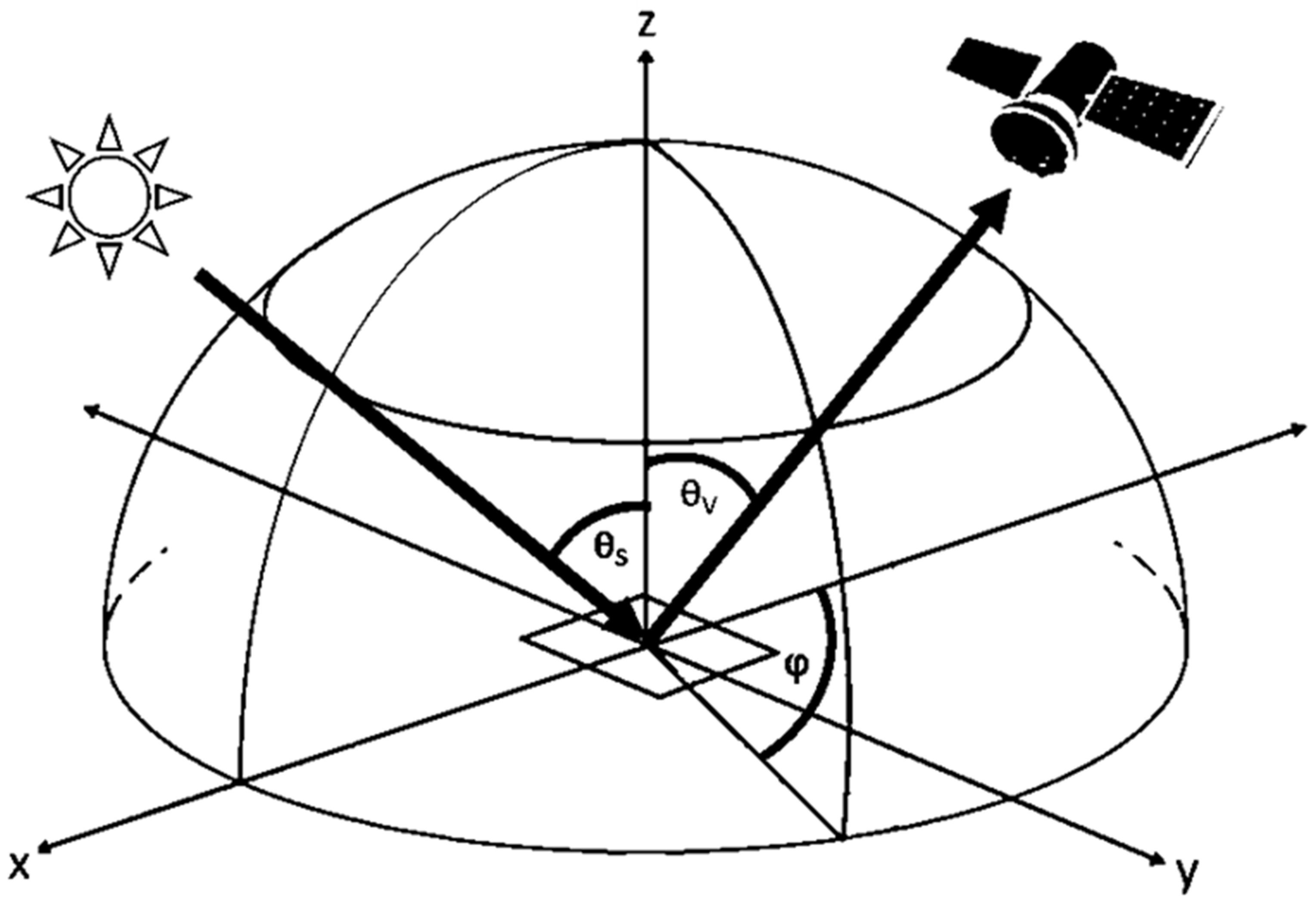
2. Theoretical Basis

While some of the finer details regarding the conversion of radiance to irradiance have evolved over time, the general approach remains the same and is outlined in this section. Irradiance $F$ is related to radiance $I$ by:

$$F\left({\theta }_S\right)={\int }_0^{2\pi }{\int }_0^{\frac{\pi }{2}}I({\theta }_S, {\theta }_V, \phi )\cos {\theta }_V\sin {\theta }_{V}d{\theta }_V{d}_{\phi }$$

(1)

where ${\theta }_S$ is the solar zenith angle, ${\theta }_V$ is the viewing zenith angle, and $\phi$ is the relative azimuth angle between the sun and the satellite (Figure 1).

For the special case of Lambertian or isotropic radiance $I_{iso}$ where the radiance does not depend on viewing geometry (${\theta }_V, \phi$), the calculation of irradiance $F$ in Equation (1) simplifies to:

$$F\left({\theta }_S\right)=\mathsf{\pi }{I}_{iso}\left({\theta }_S\right).$$

(2)

It follows that, for the more general anisotropic case, Equation (1) can be written as:

$$F\left({\theta }_S\right)=\frac{\pi I({\theta }_S, {\theta }_V, \phi )}{R({\theta }_S, {\theta }_V, \phi )},$$

(3)

where $R$ is the anisotropic function that relates radiance to irradiance. The function $R$ provides a correction to account for how much the radiance in direction (${\theta }_V, \phi$) deviates from the equivalent isotropic case; a value greater than unity would be associated with a radiance $I$ that is larger than the isotropic radiance $I_{iso}$, and vice versa.

Angular distribution models (ADMs) are, in essence, a discretized form of the anisotropic function $R$ known as anisotropic factors. In order to derive anisotropic factors, and therefore generate ADMs, an empirical approach has traditionally been adopted. Discrete angular bins are defined, and a large number of observed radiances collected over an extended time period are assigned to each of those angular bins and averaged (e.g., Figure 2).

For solar zenith angle bin $i$, viewing zenith angle bin $j$, and relative azimuthal bin $k$, the anisotropic factor $R_{ijk}$ is calculated as:

$$R_{ijk}=\frac{\pi {\overline{I}}_{ijk}}{F_i}.$$

(4)

In Equation (4), ${\overline{I}}_{ijk}$ is the mean of normalized instantaneous radiances $I_{ijk}$ in angular bin $(i, j, k)$. A normalization is applied to each instantaneous radiance observation ${I^{\prime }}_{ijk}$ to account for variations in Earth-sun distance and solar zenith angle as follows:

$$I_{ijk}={I^{\prime }}_{ijk}\frac{{\mu }_i}{{\mu }^{\prime }}{\left(\frac{r^{\prime }}{r_0}\right)}^2,$$

(5)

where ${\mu }^{\prime }$ and $r^{\prime }$ are the cosine of the solar zenith angle and the Earth-sun distance at the time of observation, respectively, ${\mu }_i$ is the cosine of the solar zenith angle at the mid-point of solar zenith angle bin $i$, and $r_0$ is the mean Earth-sun distance. Note that the instantaneous radiances ${I^{\prime }}_{ijk}$ considered in Equation (5) are assumed to be pre-processed, including spectral unfiltering and calibration [25,26,27], which is not discussed here.

The corresponding irradiance $F_i$ that appears in Equation (4) is the summation of ${\overline{I}}_{ijk}$ over all viewing zenith angle bins $j$ and all relative azimuthal angle bins $k$ using a discrete form of Equation (1) with the functional form:

$$F_i={\displaystyle \sum }_{j=1}^{N_j}{w}_j {\displaystyle \sum }_{k=1}^{N_k}{w}_k{\overline{I}}_{ijk},$$

(6)

where $N_j$ and $N_k$ are the total number of angular bins in viewing zenith angle and relative azimuth angle, respectively, and $w_j$ and $w_k$ are weights associated with the hemispheric integral. The weights can be determined analytically for certain angular bin widths, or estimated numerically with fixed angular bin widths and an additional weighting by cosine of the viewing zenith angle (e.g., via Gaussian quadrature).

Note that the entire process of deriving anisotropic factors described in this section is typically performed separately for scene types with distinct anisotropy. The choice of scene types, as well as the angular resolution, has changed dramatically over the history of ERB satellite observations, as described next.

3. Historical Review to State-of-the-Art

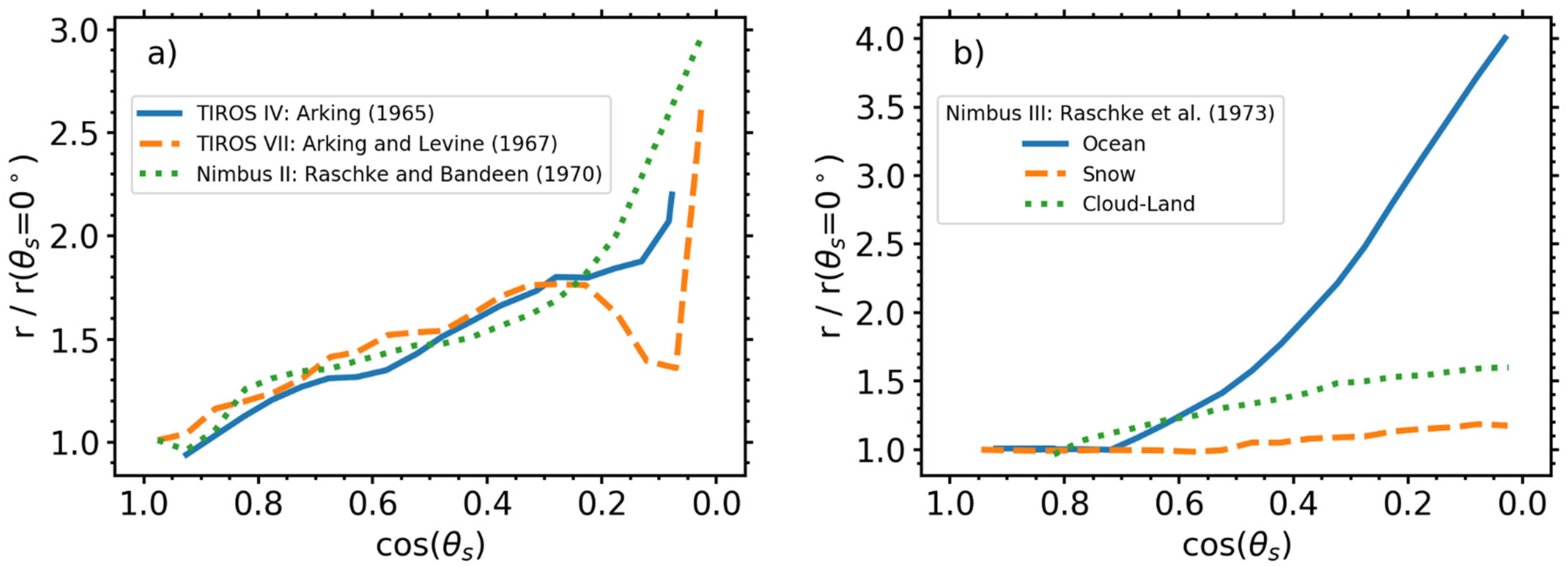
3.1. Early Satellite Analyses

The importance of accounting for variations in reflected shortwave radiation with angle has been appreciated since early in the ERB satellite era. Arking [28] and Arking and Levine [29] noted that, for constant surface and meteorological conditions, reflectance could change by a factor of 1.5 between noon (when the sun is close to overhead) and later in the afternoon when the sun is 30° above the horizon. This effect had been neglected in earlier satellite analyses [30,31], but should be accounted for when calculating time-averages of reflected shortwave radiation taken at different times in the diurnal cycle. The first models to account for this change in reflectance with solar zenith angle were derived from TIROS IV and TIROS VII satellite observations in highly inclined orbits that lacked global coverage. This was followed by analysis of observations made from the sun-synchronous Nimbus II satellite [32], which provided the first global model (Figure 3a).

A subsequent analysis of Nimbus III observations [6] was the first to account for angular variations of different scene types (Figure 3b). This included three fixed scene types of ocean, snow, and a land-cloud combination that were generated from “gross-empirical” models that used a combination of aircraft, balloons, and early satellite data. This analysis, together with the earlier seminal work of Vonder Haar and Suomi [14], had profound implications for our understanding of the climate system, including the discovery that Earth was significantly darker than most pre-satellite estimates, and that low latitudes absorbed more energy than previously thought, implying a stronger poleward heat transport by approximately 40%.

A further development came with analysis of Nimbus VII observations [3], which used 4 scenes: ocean, land, snow-ice combination, and cloud. Importantly, given the distinct anisotropy presented by clouds, the Nimbus VII analysis was the first to attempt dynamic cloud identification [33]. Observations from Nimbus VII were later used in the development of shortwave ADMs applied during the Earth Radiation Budget Experiment (ERBE) mission, as described in the next section. A summary of the early satellite analyses presented in this section is provided in

Table 1. Summary of shortwave ADMs applied to pre-ERBE satellite observations.

Mission	Analysis Period	Scene Types (# Scenes)	Notes	Reference(s)
TIROS IV	1962	Low latitudes (1)	First to account for changes in reflection with solar zenith angle	[28]
TIROS VII	1963–1964	N/A: isotropic	Isotropic assumption resulted in underestimate of albedo in polar regions	[30]
TIROS VII	1963–1964	Near-global (1)	Similar approach to TIROS IV but improved statistics	[29]
Nimbus II	1966	Global (1)	First global anisotropic function	[32]
Nimbus III	1969–1970	Ocean, snow, land-cloud combination (3)	Multiple scene types, “gross-empirical” models derived from a variety of sources including aircraft, balloons, and early satellite data	[6]
Nimbus VII	1978–1979	Ocean, land, snow-ice combination, cloud (4)	First attempt at dynamic cloud identification	[3,33]

.

3.2. ERBE

The Earth Radiation Budget Experiment (ERBE), launched in 1984, was the first multi-satellite constellation system for observing the ERB. From two sun-synchronous satellites, NOAA-9 (850 km, ascending 14:30 equator crossing) and NOAA-10 (810 km, descending 07:30 equator crossing), and a dedicated precessing satellite, the Earth Radiation Budget Satellite (ERBS; 610 km, 57° inclination), ERBE provided global coverage and sampled diurnal variability. Shortwave ADMs were never generated with ERBE observations. Instead, ERBE shortwave ADMs were generated from 205 days (1 April 1979–22 June 1980) of Nimbus VII ERB scanner observations [21] that are summarized in this section.

The ERBE ADMs included 12 scene types combining various cloud fractions over different surfaces (

Table 2. ERBE shortwave ADM scene types. Reproduced and adapted from Suttles et al. [21].

Scene ID Number	Cloud Fraction	Surface Type
1	Cloud-free (0–5%)	Ocean
2	Cloud-free (0–5%)	Land
3	Cloud-free (0–5%)	Snow
4	Cloud-free (0–5%)	Desert
5	Cloud-free (0–5%)	Land-ocean mix
6	Partly cloudy (5–50%)	Ocean
7	Partly cloudy (5–50%)	Land or desert
8	Partly cloudy (5–50%)	Land-ocean mix
9	Mostly cloudy (50–95%)	Ocean
10	Mostly cloudy (50–95%)	Land or desert
11	Mostly cloudy (50–95%)	Land-ocean mix
12	Overcast	All

). The distinct anisotropy of these scene types is shown in Figure 4. For example, at low sun the anisotropy over land and ocean in cloud-free conditions (Figure 4c,d, right half of plots) is stronger than cloud-free over snow and overcast conditions (Figure 4a,b, right half of plots) due to multiple scattering within clouds and within the snow-pack, which tends to smooth the angular distribution of reflected solar radiation. To assign each of the Nimbus VII ERB scanner radiances to a scene type for the generation of ERBE ADMs, a fixed surface type was used and a cloud detection algorithm was applied that used co-located observations from the Temperature and Humidity Infrared Radiometer (THIR) and the Total Ozone Mapping Spectrometer (TOMS), both of which were on the Nimbus VII spacecraft [34]. The Nimbus VII ERB scanner had an approximate nadir resolution of 90 $\times$ 90 km extending to more than 250 km near the limb, and therefore scene identification was unavoidably coarse. Only 9 non-mixed scene types were defined for the Nimbus VII observations; the land-ocean mixed scene types in ERBE ADMs are weighted averages of observations from each of the non-mixed scene types.

When applying ERBE ADMs, supporting observations to identify the scene type associated with each ERBE radiance observation, such as those used with Nimbus VII in the generation of the ERBE ADMs, were not available. Instead, a maximum likelihood estimation approach [36] was employed that relied only on the longwave and shortwave radiances observed by ERBE (Figure 5). The general idea was that as the cloud cover increases, the scene becomes brighter, increasing the shortwave reflectance, while the effective emitting surface is shifted higher in the atmosphere and therefore to colder temperatures, reducing the longwave emission. While this only permits a relatively simple scene identification by today’s standards, the simplicity of the ERBE approach had the advantage of not relying on a coincident imager.

For each of the ERBE scene types, 10 solar zenith angle bins were considered. Each of those were then further split into 7 viewing zenith angle bins and 8 relative azimuth angle bins (Figure 6a). The majority of angular bins for each scene type were populated with the minimum of eight Nimbus VII ERB scanner observations that were determined appropriate for a reliable angular bin average [21]. One major issue was that, due to the sun-synchronous orbit of Nimbus VII, some scenes were never observed at certain solar zenith angles. As such, all viewing zenith angle and relative azimuth angle bins for a given solar zenith angle bin over some scene types were missing. This issue was addressed with the Helmholtz reciprocity principle [38], which essentially says that the reflective characteristics of a scene (in this case, the anisotropic factors) are independent of the direction that the radiation is travelling. If this principle holds, solar zenith angle and viewing zenith angle can be interchanged. Apart from two solar zenith angle bins over the desert that were filled with an empirical model [39], any remaining missing angular bins after applying this principle were infrequent and filled with bi-linear interpolation or extrapolation.

3.3. CERES

The Clouds and the Earth’s Radiant Energy System [CERES; 5] launched its first instrument in 1997. Via 7 different instruments on 5 different low-Earth orbiting satellites, CERES continues to provide ERB satellite observations at the time of writing this paper. The extended CERES data record has permitted multiple generations of shortwave ADMs that are summarized in this section.

3.3.1. CERES-TRMM

The first CERES shortwave ADMs were generated using observations from the CERES instrument on the Tropical Rainfall Measuring Mission (TRMM) satellite, henceforth CERES-TRMM [22,40]. The TRMM satellite was in a 350 km circular orbit with an inclination angle of 35°, permitting observations from approximately 38° S–38° N after taking into account the CERES scan extent. The precessing orbit facilitated sampling of scenes within this latitude range at all solar viewing geometries, addressing some of the most serious issues of missing data experienced in the ERBE ADMs. Every third day the instrument was operated in rotating azimuth plane scan (RAPS) mode, where the instrument rotates in azimuth as it scans in elevation, to more effectively sample the angular space.

Nine months of available observations from CERES–TRMM (January–August 1998 and March 2000) were used to generate ADMs. A subtle but important update in the CERES-TRMM ADMs relative to the ERBE ADMs was that solar-viewing geometry was defined at a field-of-view reference level of 100 km above the Earth’s surface (rather than at the Earth’s surface) to account for transmission of shortwave radiation through the atmosphere beyond Earth’s horizon, and the top-of-atmosphere reference level for the irradiance was defined to be 20 km (rather than 30 km) [41]. Angular binning was similar to that used by ERBE, with 2 additional bins each in viewing zenith angle and relative azimuth angle (Figure 6b). However, by utilizing the Visible and Infrared Scanner (VIRS) instrument also flying on the TRMM satellite, a far greater number of scene types were defined (

Table 3. CERES-TRMM shortwave ADM scene types that contain cloud. Reproduced and adapted from Loeb et al. [22] © American Meteorological Society. Used with permission. The numbers in parentheses in the first column indicate the number of scene types.

Surface Type	Cloud Thermodynamic Phase	Cloud Fraction (%)	Cloud Optical Depth
Ocean (336)	Liquid, ice	0.1–10, 10–20, 20–30, 30–40, 40–50, 50–60, 60–70, 70–80, 80–90, 90–95, 95–99.9, 99.9–100	0.01–1.0, 1.0–2.5, 2.5–5.0, 5.0–7.5, 7.5–10, 10–12.5, 12.5–15, 15–17.5, 17.5–20, 20–25, 25–30, 30–40, 40–50, >50
Moderate–high tree/shrub coverage (60), low–moderate tree/shrub coverage (60), dark desert (60), bright desert (60)	Liquid, ice	0.1–25, 25–50, 50–75, 75–99.9, 99.9–100	0.01–2.5, 2.5–6, 6–10, 10–18, 18–40, >40

). Notably, cloud-free ocean scenes were additionally segregated by surface wind speed, and cloudy scenes were additionally segregated by cloud optical depth and cloud phase. This was achieved by applying thresholds to VIRS pixels within the CERES footprint for cloud detection and applying an iterative inversion for the retrieval of cloud optical depth and cloud phase [42].

An example of the additional value gained by segregating scenes with varying cloud optical depth and cloud phase is shown in Figure 7. A scene becomes more isotropic with increasing τ as a greater fraction of the photons reaching the sensor go through the multiple scattering process. While the differences in anisotropy due to cloud optical depth and phase are not as large as those of different solar zenith angle and surface type as indicated in ERBE ADMs (compare variations within Figure 7 to those within Figure 4), there is a distinct and sometimes large change in anisotropy with cloud properties. Accounting for these additional parameters therefore leads to improved regional irradiance prediction, with an estimated monthly mean uncertainty of less than 0.5 W m^–2 and an instantaneous error of less than 10 W m^–2 at the 1° $\times$ 1° scale [40]. In addition, the CERES-TRMM ADMs show improved self-consistency, as defined and discussed further in the next section.

3.3.2. CERES-Terra

The next generation of CERES shortwave ADMs were generated using observations from the Terra satellite, henceforth CERES-Terra [23,43]. Terra was launched in 1999 into a 705 km sun-synchronous orbit with a descending equator crossing at 10:30 local time (although the orbit is now starting to drift in local time). At the time of writing this paper, two CERES instruments are still operational on the Terra satellite. One of the instruments was often dedicated to RAPS mode in the initial years of flight. Two years of data from CERES-Terra were used to generate the CERES-Terra ADMs, providing at least an order of magnitude increase in angular sampling at any given solar zenith angle compared to CERES-TRMM. This allowed for a substantial increase in angular bin resolution (e.g., 2° in solar zenith, viewing zenith, and relative azimuth angles for cloud-free ocean scenes) and a further segregation of scene types. Cloud properties were inferred in a consistent manner to CERES-TRMM, but using the Moderate Resolution Imaging Spectroradiometer (MODIS) that was available on the Terra satellite instead of VIRS (

Table 4. CERES-Terra shortwave ADM scene types for permanent snow, fresh snow, and sea ice. Reproduced and adapted from Loeb et al. [23] © American Meteorological Society. Used with permission. The numbers in parentheses in the first column indicate the number of scene types.

Surface Type	Cloud Fraction (%)	Surface Brightness	Snow/Sea Ice Fraction (%)	Cloud Optical Depth
Permanent snow (10)	0.0–0.1	Bright, dark *	-	-
	0.1–25	All	-	All
	25–50	All	-	All
	50–75	All	-	All
	75–99.9	All	-	All
	99.9–100	Bright, dark *	-	Thin (τ ≤ 10), thick (τ > 10)
Fresh snow (25), sea ice (25)	0.0–0.1	All	0.0–0.1	-
	0.0–0.1	All	0.1–25	-
	0.0–0.1	All	25–50	-
	0.0–0.1	All	50–75	-
	0.0–0.1	All	75–99.9	-
	0.0–0.1	Bright, dark *	99.9–100	-
	0.1–25	All	0.0–0.1	All
	0.1–25	All	0.1–25	All
	0.1–25	All	25–50	All
	0.1–25	All	50–75	All
	0.1–25	All	75–99.9	All
	25–50	All	0.0–0.1	All
	25–50	All	0.1–25	All
	25–50	All	25–50	All
	25–50	All	50–75	All
	50–75	All	0.0–0.1	All
	50–75	All	0.1–25	All
	50–75	All	25–50	All
	75–99.9	All	0.0–0.1	All
	75–99.9	All	0.1–25	All
	99.9–100	Bright, dark *	All	Thin (τ ≤ 10), thick (τ > 10)

* Surface brightness was determined by comparing each CERES observation with a monthly regional snow map that classifies all 1° $\times$ 1° regions with snow/sea ice as either bright or dark [44].

).

For CERES-Terra, separate ADMs were defined over cloud-free land and desert for each 1° $\times$ 1° region, for each month, and for normalized difference vegetation index (NDVI) differing by 0.1. Instead of the traditional sorting-by-angular-bins method, an eight parameter fit was applied to model the bidirectional reflectance distribution function for these scenes [45]. An additional 60 scenes were defined over snow and ice (Table 4) using angular bins of 2° or 5° in solar zenith angle, and 5° in viewing zenith and relative azimuth angles. For cloudy scenes, CERES-Terra ADMs took a distinctly different approach. Over ocean, sigmoidal functions were fit between $\ln \left(f\tau \right)$ and the shortwave radiance in 2° angular bins for liquid, ice, and mixed phase cloud, where $f$ is the cloud fraction and $\tau$ is the cloud optical depth (Figure 8). A similar approach was taken over land, but coarser 5° angular bins and an additional correction to account for the surface reflection was applied. Under this definition, the cloudy scenes essentially become continuous, and the number of scene types is therefore more difficult to quantify from this point forward.

As an approach to validate both the CERES-TRMM and CERES-Terra shortwave ADMs, it was noted that the average all-sky albedo at a given solar zenith angle should be independent of satellite viewing geometry. This provided a useful consistency test. Both the CERES-TRMM and CERES-Terra ADMs show improved self-consistency compared with ERBE ADMs (Figure 9). While ERBE ADMs show 4–8% variation in albedo with viewing zenith angle, CERES-TRMM and CERES-Terra ADMs show variations closer to 1–2% [40,43].

3.3.3. CERES-Terra/Aqua

The most recent CERES ADMs have been developed using an extended record of 5 years of RAPS data from the Terra satellite combined with 1 year and 8 months of RAPS data from the Aqua satellite, henceforth CERES-Terra/Aqua [24,46]. The Aqua satellite launched in 2002 and, similar to Terra, hosts two CERES instruments that remain in orbit at the time of writing this paper. Aqua also flies in a 705 km sun-synchronous orbit, but with an ascending equator crossing at 13:30 local time (although the orbit is due to start drifting in local time in 2022). Separate ADMs are developed for Terra and Aqua over all scenes except permanent snow and sea ice. The approach applied is similar to CERES-Terra with a few key updates. For cloud-free scenes over ocean, the scene types are further segregated by aerosol optical depth in glint regions, and both aerosol optical depth and two aerosol types (rural and urban [47]) in non-glint regions. For cloud-free over land and fresh snow, the Ross-Li BRDF model [48,49] is used that contains terms to account for an isotropic contribution, randomly distributed and oriented protrusions, and radiative transfer within a vegetation canopy that includes the hotspot effect. For permanent snow, separate shortwave ADMs are generated for Antarctica and Greenland due to the effects of elongated dune-like features in the snow, known as sastrugi, that are only found on Antarctica [50]. For sea ice, there is additional segregation by the brightness of the sea ice (

Table 5. CERES-Terra/Aqua shortwave ADM scene types for sea ice. Reproduced and adapted from Su et al. [24] © American Meteorological Society. Used with permission. The numbers in parentheses in the first column indicate the number of scene types.

Cloud Fraction (%)	Sea Ice Fraction (%)	Surface Brightness	Cloud Optical Depth	Cloud Phase
0–1 (8)	0.0–1	All	-	-
	1–25	All	-	-
	25–50	All	-	-
	50–75	All	-	-
	75–99	All	-	-
	99–100	Dark, mid, bright *	-	-
1–25 (8), 25–50 (8), 50–75 (8)	0.0–1	All	All	All
	1–25	All	All	All
	25–50	All	All	All
	50–75	All	All	All
	75–99	All	All	All
	99–100	Dark, mid, bright *		All
75–99 (16)	0.0–1	All	$\ln \tau$ < 1, $\ln \tau$ ≥ 1	All
	1–25	All	$\ln \tau$ < 1, $\ln \tau$ ≥ 1	All
	25–50	All	$\ln \tau$ < 1, $\ln \tau$ ≥ 1	All
	50–75	All	$\ln \tau$ < 1, $\ln \tau$ ≥ 1	All
	75–99	All	$\ln \tau$ < 1, $\ln \tau$ ≥ 1	All
	99–100	Dark, mid, bright *	$\ln \tau$ < 1, $\ln \tau$ ≥ 1	All
99–100 (N/A)	All	0–0.6	Continuous in $\ln \tau$	Liquid, ice *
	All	0.6–0.7	Continuous in $\ln \tau$	Liquid, ice *
	All	0.7–0.8	Continuous in $\ln \tau$	Liquid, ice *
	All	0.8–0.9	Continuous in $\ln \tau$	Liquid, ice *
	All	0.9–1.0	Continuous in $\ln \tau$	Liquid, ice *

* Surface brightness and cloud phase are determined based on thresholds applied to a sea ice brightness index and effective cloud phase index, respectively [24].

), which accounts for variations in anisotropy due to features such as melt ponds (Figure 10). The presence of melt ponds reduces the overall albedo of the surface, but the liquid water has stronger anisotropy than the underlying ice surface (c.f., Figure 4). Improved cloud algorithms are employed [51] that include the addition of the 1.24 μm channel for cloud optical depth retrieval over snow, a CO2-slicing method to retrieve high cloud over low cloud [52], and a rough ice crystal model [53].

The accuracy of shortwave irradiance estimated by CERES-Terra/Aqua ADMs was evaluated by Su et al. [46] using direct integration and irradiance consistency tests. Direct integration tests, which involve directly integrating the observed radiances over a given region and comparing them to the ADM-estimated irradiance, show that the overall bias in regional monthly mean top-of-atmosphere shortwave irradiance is less than 0.2 W m^–2 and the root-mean-square-error (RMSE) is less than 1.1 W m^–2. The bias and RMSE were found to be very similar between Terra and Aqua. Irradiance consistency tests were used to assess the accuracy of instantaneous irradiance, which involve comparing irradiance estimated from nadir and oblique viewing angles using CERES along-track observations and temporally and spatially matched MODIS observations, and using irradiance converted from multi-angle MISR observations. The averaged top-of-atmosphere instantaneous shortwave irradiance uncertainties from these two tests were found to be about 2% for cloud-free scenes, and around 2.7% to 3.7% for all-sky scenes. In general, the top-of-atmosphere shortwave irradiance uncertainties were larger for thin broken clouds than for moderate and thick overcast clouds.

3.4. Application to Other Instruments

Empirical ADMs can be, and have been, adapted and applied to convert radiance to irradiance for satellite instruments other than those for which they were designed. Examples include other low-Earth orbiting satellites such as the Scanner for Radiation Budget (ScaRaB) instrument of the Megha-Tropiques mission [54,55], and the Broadband Radiometer (BBR) of the planned EarthCARE mission [56,57]. Here, we highlight two applications from different orbits: the Geostationary Earth Radiation Budget (GERB) instruments on board the Meteosat Second Generation (MSG) satellites, and the National Institute of Standards and Technology Advanced Radiometer (NISTAR) and Earth Polychromatic Imaging Camera (EPIC) on the Deep Space Climate Observatory (DSCOVR).

The GERB instruments [58] provide a unique vantage point from geostationary orbit, where the MSG satellites orbit the Earth at the same rate as Earth’s rotation and therefore continuously sample the same locations, well suited for observing and understanding the diurnal evolution of the ERB [59]. Since each location within the GERB field-of-view is always sampled at the same viewing geometry, accurate ADMs are crucial for the conversion of GERB radiance to irradiance. This conversion is performed for GERB shortwave observations using the CERES-TRMM ADMs. The scene type is determined based on a fixed surface-type map and the results of a real-time cloud detection, phase, and optical depth retrieval algorithm [60,61] applied to narrowband observations from the Spinning Enhanced Visible and Infrared Imager (SEVIRI) instrument on the same MSG satellite [62]. The SEVIRI observations are angularly matched with GERB and have a compatible temporal (~15 min) resolution but a higher spatial resolution (~3km at nadir). To lessen the impact of the resolution differences between GERB and the observations used to generate the CERES-TRMM ADMs, the ADMs are not assigned at the GERB pixel scale (~50 km at nadir), but rather on sub-regions within each GERB footprint corresponding to 3 $\times$ 3 SEVIRI pixels (~9 km at nadir). The fixed view geometry of the GERB instrument means that view angle specific errors will introduce regional biases that do not cancel over time. While empirical ADMs alleviate this problem, issues can remain for certain scenes due to limited sampling in the ADMs, observational conditions specific to the region, or geometry-based biases in scene identification. For GERB, the prevalence of Saharan dust within the field-of-view has been shown to significantly influence the conversion from shortwave radiance to irradiance, introducing a mean bias of 2.5 W m⁻² and much larger instantaneous, but compensating, differences [63]. Other shortwave radiance to irradiance conversion biases of several percent are also known to occur in the GERB products at low aerosol loadings over cloud-free ocean, for viewing geometries that are particularly sensitive to the effects of ocean wind speed or are close to the ocean glint angle at which specular reflection occurs [64].

The DSCOVR provides another unique view of ERB from the Lagrange-1 point where it orbits the Sun at the same rate as the Earth, and therefore provides continuous monitoring of the sunlit side of the Earth. On board, the NISTAR observes the entire Earth-integrated radiance in total, shortwave, and near-infrared channels while the EPIC simultaneously provides imagery in 10 narrow bands. Although the Earth rotates through the field-of-view of these instruments, each location within the field-of-view is continuously sampled at almost the same solar-viewing geometry in a very narrow back-scatter direction, so ADMs are arguably even more critical than for GERB. Anisotropic factors from the CERES-Terra/Aqua ADMs have been applied to EPIC imagery, where shortwave radiances were derived using relationships between similar narrowband channels on MODIS and the CERES shortwave radiance, and scene type was determined using low-Earth orbiting and geostationary satellite imager retrievals [65]. The global-mean daytime anisotropic factors from the EPIC analysis have also been applied to the NISTAR unfiltered radiances [66]. These studies concluded that daily mean EPIC and CERES shortwave irradiance agree to within 2%, which is within calibration and algorithm uncertainties, indicating that the calculation of global anisotropic factors from the CERES-Terra/Aqua ADMs is robust, while annual-mean NISTAR shortwave irradiances are about 6% larger than those from CERES but their diurnal variations are highly correlated.

4. Recent Advances That Support and Build Upon Existing Approaches

4.1. Machine Learning

While ADMs generated using observations from the CERES instruments (Section 3.3) have benefited from detailed scene information provided by an accompanying imager, one implication is that application of these ADMs has become somewhat dependent on availability of the imager information. For previous ERB instruments on spacecraft that do not have an imager, or for potential future ERB instruments on small satellites or constellations of such satellites that are unlikely to include an imager [67,68], these ADMs are therefore not directly applicable. Even when an ERB instrument is flying with an imager, the imager coverage over a radiometer footprint can be unreliable particularly over polar regions (less than 2% of the CERES-Terra/Aqua footprints have insufficient imager information [24]) or the imager flying with the ERB instrument can fail prematurely. As such, approaches for the conversion from shortwave radiance to irradiance that do not require complex imager information remain desirable.

The enormous data volume now available from decades of ERB satellite observations is attractive for machine learning approaches. For CERES-TRMM and CERES-Terra ADMs, an artificial neural network (ANN) has been applied to estimate irradiance [69,70]. In these studies, shortwave anisotropic factors were predicted using only the solar-viewing geometry and the shortwave and longwave radiances observed by CERES. The global annual-mean bias introduced by the ANN-derived irradiance was found to be less than 0.5% for all surface types, and the ANN-derived irradiance still maintained self-consistency in viewing zenith angle better than ERBE ADMs (c.f., Figure 9). This ANN approach is currently used operationally as a backup for CERES footprints with insufficient imager information to avoid systematic biases from omitting these footprints.

Rather than predict the anisotropic factors directly, it is also possible to predict the scene type using machine learning. Thampi et al. [71] used a random forest to classify CERES footprints as cloudy or cloud-free over 10 different surface types. The daytime misclassification rate varied with surface type and was typically >10% over bright surfaces. However, when thin cloud cases were excluded from the analysis, the daytime misclassification rate reduced to <4% for almost all surface types and was most often below 1%. The most important predictor for all surface types was the CERES shortwave radiance, indicating that the footprint-scale radiances contain valuable information on the scene type, and therefore demonstrating the potential of machine learning for scene classification without imager information.

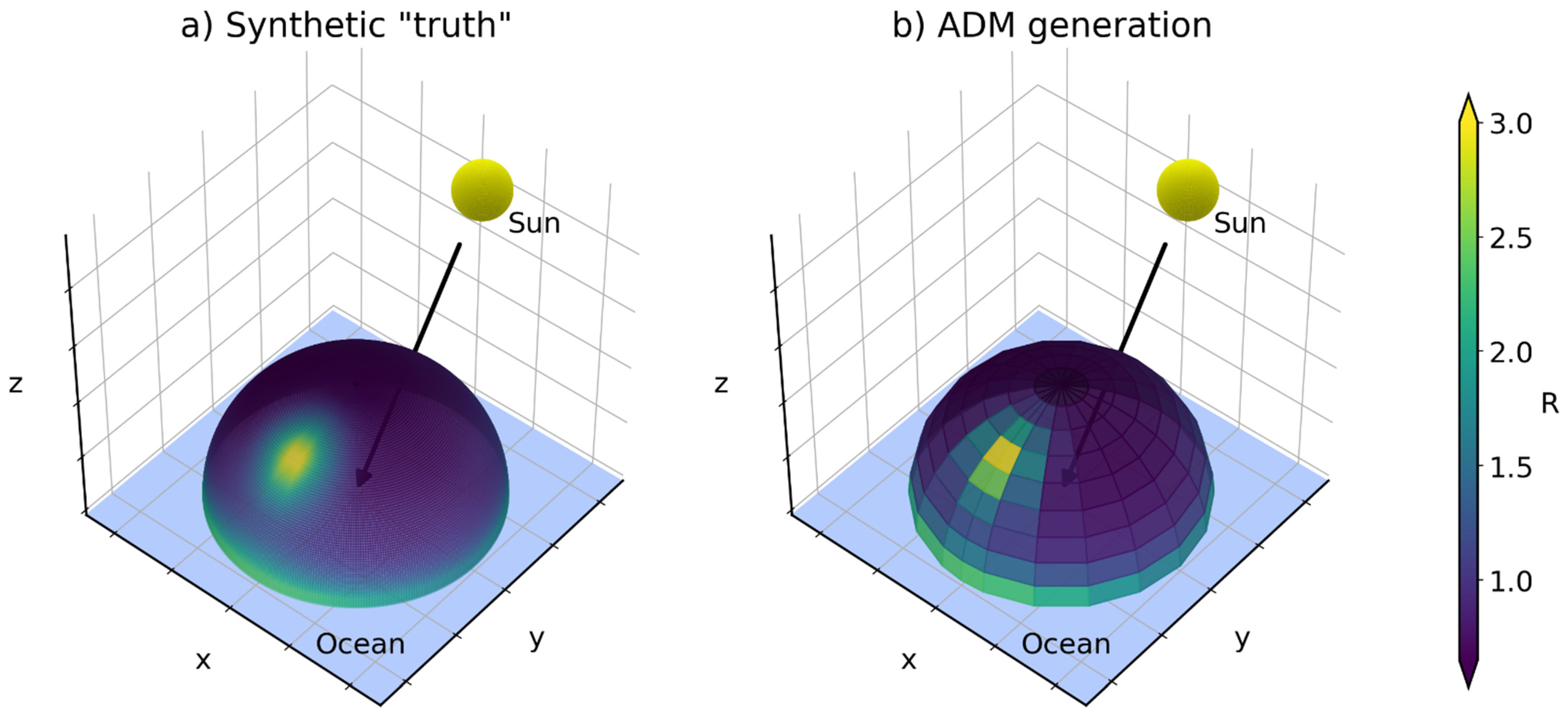
4.2. Semi-Physical Approach

As evident in the evolution of CERES ADMs (Section 3.3), further segregation of scene type, by using additional scene parameters, may allow further reduction in the uncertainty of instantaneous irradiance estimates. Semi-physical ADMs that were recently developed for clouds over ocean [72] include two additional atmospheric parameters beyond the traditionally used cloud fraction, phase, and optical depth:

(1) MODIS cloud-top effective radius, $R_e$: as known from Mie theory, the angular distribution of light scattered from a water droplet or ice crystal is related to the particle size, and therefore the particle size may affect top-of-atmosphere anisotropy of cloudy scenes as a whole.

(2) Reanalysis-based above-cloud water vapor: gaseous absorption increases with absorber mass (here vertically integrated water vapor mixing ratio between cloud-top and top-of-atmosphere) and atmospheric path length, affecting greater viewing zenith angles more strongly and, thus, impacting top-of-atmosphere anisotropy.

For training the semi-physical ADMs, the approach uses the same data as CERES-Terra/Aqua ADMs (see Section 3.3.3) plus collocated profiles from ERA-20C, and only mildly increases statistical complexity (this approach has six free parameters instead of five required for each sigmoidal curve). This is possible by using a physical framework that is then statistically optimized for each angular bin. It incorporates (1) the functional form of two-stream cloud albedo that essentially produces a sigmoidal curve and includes the asymmetry parameter $g$, which is then functionally linked to MODIS-based $R_e$. (2) The ocean reflectance anticipated in cloud-free portions of a footprint is described by the Cox-Munk model [73]. An approximate footprint albedo [i.e., the area-weighted mean of up to two cloud layers using (1) and of cloud-free portions using (2)] is then multiplied by an exponential term to resemble water vapor attenuation. Figure 11a shows an example of the variation in shortwave anisotropic factors as a function of $R_e$. Like CERES-Terra/Aqua ADMs, the semi-physical approach discriminates between footprints containing clouds that consist of liquid, ice, or both. In contrast to CERES-Terra/Aqua ADMs, this approach allows to proportion ice and liquid fractions when both phases are present. Compared against CERES-Terra/Aqua ADMs and indicative of added explanatory power, radiance residuals are reduced in most angular bins outside the sun-glint region and mostly for footprints consisting of liquid, and both liquid and ice clouds. On the other hand, the glint region as well as geometries that are sparsely sampled remain best captured using a fully statistical approach.

When applying the semi-physical ADMs to liquid clouds observed by CERES-MODIS and GERB-SEVIRI over the course of two months, the resulting instantaneous fluxes differed by up to 25 W m^–2 relative to those reproduced by CERES-Terra/Aqua ADMs [74]. As shown for selected $R_e$ in Figure 11b–d, the sharpest corresponding anisotropy differences (equivalent to peak relative differences of ±5%) are non-monotonic and occur mainly in the backscattering direction associated with single scattering features such as cloud bow and cloud glory (curved features in the top half of the polar plots) as well as the forward scattering direction (predominantly multi-scattering; broad features in the bottom half of the polar plots). These differences propagated into the daily and monthly mean of instantaneous irradiances at the 1° × 1° scale (up to ±10 and ±5 W m^–2, respectively), predominantly in regions of persistently extreme values of $R_e$ (smaller than 7 μm or larger than 15 μm) or above-cloud water vapor (not shown).

5. Summary and Conclusions

The conversion of shortwave radiance observed by ERB satellite instruments to shortwave irradiance is an essential processing step to obtain the energetically relevant data needed to monitor and understand our climate system. The related underlying theory has been leveraged to develop models over a series of decades that provide a route to convert between radiance and irradiance, known as ADMs. An empirical approach has traditionally been taken to generate ADMs: radiances collected over an extended time period at a large range of solar-viewing geometries are sorted into angular bins and averaged, a process that is performed separately for scene types with distinct anisotropy. As the ERB observing system has evolved over time, instruments have observed for longer duration and have flown with more advanced imagers, leading to a substantial increase in the complexity and capability of shortwave ADMs over time.

Early analyses applied to ERB observations from the 1960s and 1970s, including instruments on the TIROS and Nimbus series of satellites, were relatively coarse in their treatment of the angular distribution of reflected shortwave radiation. It was first noted that variations in solar zenith angle could significantly alter the reflectance of an identical scene, followed by recognition that the shortwave anisotropy depends on the scene properties themselves. By the end of the Nimbus ERB record, the anisotropy of a handful of scene types were treated separately, including dynamic cloud identification that was a major step forward due to the distinct anisotropy presented by clouds. Shortwave ADMs applied during the subsequent ERBE mission additionally accounted for variations in cloud fraction to better represent the relative contribution of cloudy and cloud-free portions of a scene. Of note, the cloud fraction was retrieved using only the ERBE shortwave and longwave radiances. The following CERES mission, which is continuing to provide ERB observations at the time of writing this paper, instead takes advantage of co-flying imagers that were launched along with the CERES instruments. The extended CERES data record of over 20 years has provided multiple generations of shortwave ADMs. CERES-TRMM ADMs involved further segregation of scene types by new variables including cloud optical depth, cloud phase, and surface wind speed over cloud-free ocean. CERES-Terra ADMs extended this approach using observations with global coverage over multiple years, and introduced cloudy ADMs that are continuous in scene type. The most recent CERES-Terra/Aqua ADMs incorporate further updates including segregation by aerosol amount and type over cloud-free ocean, the effects of sastrugi, and variations in sea ice brightness. Validation efforts have shown progressively lower uncertainty in radiance to irradiance conversion with each generation of shortwave ADMs. In addition, the ADMs from CERES have been successfully adapted and applied to observations from other ERB instruments, including those in drastically different orbits.

Recent advances that support and build on these state-of-the-art shortwave ADMs include machine learning and semi-physical approaches. Machine learning of either the anisotropic factors or the scene type has been shown to produce promising results that can be applied in the absence of imager information. This is currently used operationally in CERES data processing when imager retrievals are missing. Semi-physical approaches have demonstrated that further combining theory with the traditional empirical approach can help to represent the additional influence of unaccounted variables in cloudy scenes over ocean such as above cloud water vapor and cloud drop effective radius. This demonstrates that shortwave ADMs developed for ERB can be applied more broadly, and possibly even to other remote sensing applications involving observations of anisotropic scenes.

Looking forward, continuity of the high-quality ERB data record will be crucial. As such, consistent processing of ERB observations to produce a backward compatible ERB data record, including the application of shortwave ADMs, should be a priority. The recently selected Libera mission that will continue the CERES ERB data record recognizes this requirement by matching the CERES observation strategy very closely. Libera is planned to fly alongside the Visible Infrared Imaging Radiometer Suite (VIIRS) on the Joint Polar Satellite System-3 (JPSS-3) satellite, which is scheduled to launch by December 2027. In addition to continuity goals, Libera will also explore a different proof-of-concept approach that will utilize a WFOV camera to develop ADMs for the new split-shortwave channel. This approach will be explored further in subsequent studies.

References

1. Stephens, G.L.; O’Brien, D.; Webster, P.J.; Pilewski, P.; Kato, S.; Li, J. The albedo of Earth. Rev. Geophys. 2015, 53, 141–163. [Google Scholar] [CrossRef] [Green Version]
2. Ackerman, S.A.; Platnick, S.; Bhartia, P.K.; Duncan, B.; L’Ecuyer, T.; Heidinger, A.; Skofronick-Jackson, G.; Loeb, N.; Schmit, T.; Smith, N. Satellites See the World’s Atmosphere. Meteorol. Monogr. 2019, 59, 4.1–4.53. [Google Scholar] [CrossRef]
3. Jacobowitz, H.; Soule, H.V.; Kyle, H.L.; House, F.B. The Earth Radiation Budget (ERB) Experiment: An overview. J. Geophys. Res. Atmos. 1984, 89, 5021–5038. [Google Scholar] [CrossRef]
4. Barkstrom, B.R. The Earth Radiation Budget Experiment (ERBE). Bull. Am. Meteorol. Soc. 1984, 65, 1170–1185. [Google Scholar] [CrossRef]
5. Wielicki, B.A.; Barkstrom, B.R.; Harrison, E.F.; Lee, R.B.; Louis Smith, G.; Cooper, J.E. Clouds and the Earth’s Radiant Energy System (CERES): An Earth Observing System Experiment. Bull. Am. Meteorol. Soc. 1996, 77, 853–868. [Google Scholar] [CrossRef] [Green Version]
6. Raschke, E.; Vonder Haar, T.H.; Bandeen, W.R.; Pasternak, M. The Annual Radiation Balance of the Earth-Atmosphere System During 1969–70 from Nimbus 3 Measurements. J. Atmos. Sci. 1973, 30, 341–364. [Google Scholar] [CrossRef] [Green Version]
7. House, F.B.; Gruber, A.; Hunt, G.E.; Mecherikunnel, A.T. History of satellite missions and measurements of the Earth Radiation Budget (1957–1984). Rev. Geophys. 1986, 24, 357–377. [Google Scholar] [CrossRef]
8. Dewitte, S.; Clerbaux, N. Measurement of the Earth Radiation Budget at the Top of the Atmosphere—A Review. Remote Sens. 2017, 9, 1143. [Google Scholar] [CrossRef] [Green Version]
9. Wong, T.; Smith, G.L.; Kato, S.; Loeb, N.G.; Kopp, G.; Shrestha, A.K. On the Lessons Learned from the Operations of the ERBE Nonscanner Instrument in Space and the Production of the Nonscanner TOA Radiation Budget Data Set. IEEE Trans. Geosci. Remote Sens. 2018, 56, 5936–5947. [Google Scholar] [CrossRef]
10. Stephens, G.L.; Li, J.; Wild, M.; Clayson, C.A.; Loeb, N.; Kato, S.; L’Ecuyer, T.; Stackhouse, P.W.; Lebsock, M.; Andrews, T. An update on Earth’s energy balance in light of the latest global observations. Nat. Geosci. 2012, 5, 691–696. [Google Scholar] [CrossRef]
11. Trenberth, K.E. An imperative for climate change planning: Tracking Earth’s global energy. Curr. Opin. Environ. Sustain. 2009, 1, 19–27. [Google Scholar] [CrossRef] [Green Version]
12. Wild, M.; Folini, D.; Hakuba, M.Z.; Schär, C.; Seneviratne, S.I.; Kato, S.; Rutan, D.; Ammann, C.; Wood, E.F.; König-Langlo, G. The energy balance over land and oceans: An assessment based on direct observations and CMIP5 climate models. Clim. Dyn. 2015, 44, 3393–3429. [Google Scholar] [CrossRef] [Green Version]
13. Loeb, N.G.; Wielicki, B.A. Satellites and Satellite Remote Sensing: Earth’s Radiation Budget. In Encyclopedia of Atmospheric Sciences, 2nd ed.; Elsevier Inc.: Amsterdam, The Netherlands, 2015; pp. 67–76. ISBN 9780123822260. [Google Scholar]
14. Vonder Haar, T.H.; Suomi, V.E. Measurements of the Earth’s Radiation Budget from Satellites During a Five-Year Period. Part I: Extended Time and Space Means. J. Atmos. Sci. 1971, 28, 305–314. [Google Scholar] [CrossRef] [Green Version]
15. Kramer, R.J.; He, H.; Soden, B.J.; Oreopoulos, L.; Myhre, G.; Forster, P.M.; Smith, C.J. Observational Evidence of Increasing Global Radiative Forcing. Geophys. Res. Lett. 2021, 48, e2020GL091585. [Google Scholar] [CrossRef]
16. Myers, T.A.; Scott, R.C.; Zelinka, M.D.; Klein, S.A.; Norris, J.R.; Caldwell, P.M. Observational constraints on low cloud feedback reduce uncertainty of climate sensitivity. Nat. Clim. Chang. 2021, 11, 501–507. [Google Scholar] [CrossRef]
17. Forster, P.M.F.; Gregory, J.M. The Climate Sensitivity and Its Components Diagnosed from Earth Radiation Budget Data. J. Clim. 2006, 19, 39–52. [Google Scholar] [CrossRef]
18. Hartmann, D.L.; Ceppi, P. Trends in the CERES Dataset, 2000–2013: The Effects of Sea Ice and Jet Shifts and Comparison to Climate Models. J. Clim. 2014, 27, 2444–2456. [Google Scholar] [CrossRef] [Green Version]
19. Tett, S.F.B.; Mineter, M.J.; Cartis, C.; Rowlands, D.J.; Liu, P. Can Top-of-Atmosphere Radiation Measurements Constrain Climate Predictions? Part I: Tuning. J. Clim. 2013, 26, 9348–9366. [Google Scholar] [CrossRef] [Green Version]
20. Tett, S.F.B.; Rowlands, D.J.; Mineter, M.J.; Cartis, C. Can Top-of-Atmosphere Radiation Measurements Constrain Climate Predictions? Part II: Climate Sensitivity. J. Clim. 2013, 26, 9367–9383. [Google Scholar] [CrossRef] [Green Version]
21. Suttles, J.; Green, R.; Minnis, P.; Smith, G.; Staylor, W.; Wielicki, B.; Walker, I.; Young, D.; Taylor, V.; Stowe, L. Angular Radiation Models for Earth-Atmosphere Systems, Vol. I Shortwave Radiation; NASA Reference Publication 1184; NASA: Hampton, VA, USA, 1988. [Google Scholar]
22. Loeb, N.G.; Manalo-Smith, N.; Kato, S.; Miller, W.F.; Gupta, S.K.; Minnis, P.; Wielicki, B.A. Angular Distribution Models for Top-of-Atmosphere Radiative Flux Estimation from the Clouds and the Earth’s Radiant Energy System Instrument on the Tropical Rainfall Measuring Mission Satellite. Part I: Methodology. J. Appl. Meteorol. 2003, 42, 240–265. [Google Scholar] [CrossRef]
23. Loeb, N.G.; Kato, S.; Loukachine, K.; Manalo-Smith, N. Angular Distribution Models for Top-of-Atmosphere Radiative Flux Estimation from the Clouds and the Earth’s Radiant Energy System Instrument on the Terra Satellite. Part I: Methodology. J. Atmos. Ocean. Technol. 2005, 22, 338–351. [Google Scholar] [CrossRef]
24. Su, W.; Corbett, J.; Eitzen, Z.; Liang, L. Next-generation angular distribution models for top-of-atmosphere radiative flux calculation from CERES instruments: Methodology. Atmos. Meas. Tech. 2015, 8, 611–632. [Google Scholar] [CrossRef] [Green Version]
25. Loeb, N.G.; Manalo-Smith, N.; Su, W.; Shankar, M.; Thomas, S. CERES top-of-atmosphere earth radiation budget climate data record: Accounting for in-orbit changes in instrument calibration. Remote Sens. 2016, 8, 182. [Google Scholar] [CrossRef] [Green Version]
26. Loeb, N.G.; Priestley, K.J.; Kratz, D.P.; Geier, E.B.; Green, R.N.; Wielicki, B.A.; Hinton, P.O.; Nolan, S.K. Determination of Unfiltered Radiances from the Clouds and the Earth’s Radiant Energy System Instrument. J. Appl. Meteorol. 2001, 40, 822–835. [Google Scholar] [CrossRef]
27. Priestley, K.J.; Barkstrom, B.R.; Lee, R.B.; Green, R.N.; Thomas, S.; Wilson, R.S.; Spence, P.L.; Paden, J.; Pandey, D.K.; Al-Hajjah, A. Postlaunch Radiometric Validation of the Clouds and the Earth’s Radiant Energy System (CERES) Proto-Flight Model on the Tropical Rainfall Measuring Mission (TRMM) Spacecraft through 1999. J. Appl. Meteorol. 2000, 39, 2249–2258. [Google Scholar] [CrossRef]
28. Arking, A. The Angular Distribution of Scattered Radiation and the Earth Albedo as Observed from TIROS. Annu. Res. Rep. Goddard Inst. Sp. Stud. 1965, 1, 47–67. [Google Scholar]
29. Arking, A.; Levine, J.S. Earth Albedo Measurements: July 1963 to June 1964. J. Atmos. Sci. 1967, 24, 721–724. [Google Scholar] [CrossRef] [Green Version]
30. Bandeen, W.R.; Halev, M.E.; Strange, I. A Radiation Climatology in the Visible and Infrared from the Tiros Meteorological Satellites; NASA Tech. Note D-2534; National Aeronautics and Space Administration: Washington, DC, USA, 1965. [Google Scholar]
31. Rasool, S.I.; Prabhakara, C. Heat budget of the Southern Hemisphere. In Problems of Atmospheric Circulation; Garcia, R.V., Malone, T.F., Eds.; Spartan Books: New York, NY, USA, 1966; pp. 76–92. [Google Scholar]
32. Raschke, E.; Bandeen, W.R. The Radiation Balance of the Planet Earth from Radiation Measurements of the Satellite Nimbus II. J. Appl. Meteorol. 1970, 9, 215–238. [Google Scholar] [CrossRef]
33. Taylor, V.R.; Stowe, L.L. Reflectance characteristics of uniform Earth and cloud surfaces derived from NIMBUS-7 ERB. J. Geophys. Res. Atmos. 1984, 89, 4987–4996. [Google Scholar] [CrossRef]
34. Stowe, L.L.; Wellemeyer, C.G.; Eck, T.F.; Yeh, H.Y.M. The Nimbus-7 CLOUD DATA PROCecessing TEAM Nimbus-7 Global Cloud Climatology. part I: Algorithms and Validation. J. Clim. 1988, 1, 445–470. [Google Scholar] [CrossRef] [Green Version]
35. Kidder, S.Q.; Vonder Haar, T.H. Satellite Meteorology: An Introduction; Elsevier Press: Amsterdam, The Netherlands, 1995; p. 466. [Google Scholar]
36. Wielicki, B.A.; Green, R.N. Cloud Identification for ERBE Radiative Flux Retrieval. J. Appl. Meteorol. 1989, 28, 1133–1146. [Google Scholar] [CrossRef] [Green Version]
37. Smith, G.L.; Green, R.N.; Raschke, E.; Avis, L.M.; Suttles, J.T.; Wielicki, B.A.; Davies, R. Inversion methods for satellite studies of the Earth’s Radiation Budget: Development of algorithms for the ERBE Mission. Rev. Geophys. 1986, 24, 407. [Google Scholar] [CrossRef]
38. Chandrasekhar, S. Radiative Transfer; Dover Publications: New York, NY, USA, 1960. [Google Scholar]
39. Staylor, W.F.; Suttles, J.T. Reflection and emission models for deserts derived from Nimbus-7 ERB scanner measurements. J. Clim. Appl. Meteorol. 1986, 25, 196–202. [Google Scholar] [CrossRef] [Green Version]
40. Loeb, N.G.; Loukachine, K.; Manalo-Smith, N.; Wielicki, B.A.; Young, D.F. Angular distribution models for top-of tmosphere radiative flux estimation from the clouds and the Earth’s Radiant Energy system instrument on the Tropical Rainfall Measuring Mission satellite. Part II: Validation. J. Appl. Meteorol. 2003, 42, 1748–1769. [Google Scholar] [CrossRef]
41. Loeb, N.G.; Kato, S.; Wielicki, B.A. Defining top-of-the-atmosphere flux reference level for earth radiation budget studies. J. Clim. 2002, 15, 3301–3309. [Google Scholar] [CrossRef]
42. Minnis, P.; Young, D.F.; Wielicki, B.A.; Heck, P.W.; Dong, X.; Stowe, L.L.; Welch, R.M. CERES cloud properties derived from multispectral VIRS data. In Proceedings of the Satellite Remote Sensing of Clouds and the Atmosphere IV, 20–22 September 1999; Russell, J.E., Ed.; SPIE: Florence, Italy, 1999; Volume 3867, pp. 91–102. [Google Scholar]
43. Loeb, N.G.; Kato, S.; Loukachine, K.; Manalo-Smith, N.; Doelling, D.R. Angular distribution models for top-of-atmosphere radiative flux estimation from the Clouds and the Earth’s Radiant Energy System instrument on the Terra Satellite. Part II: Validation. J. Atmos. Ocean. Technol. 2007, 24, 564–584. [Google Scholar] [CrossRef]
44. Kato, S.; Loeb, N.G. Top-of-atmosphere shortwave broadband observed radiance and estimated irradiance over polar regions from Clouds and the Earth’s Radiant Energy System (CERES) instruments on Terra. J. Geophys. Res. Atmos. 2005, 110, 1–16. [Google Scholar] [CrossRef]
45. Ahmad, S.P.; Deering, D.W. A simple analytical function for bidirectional reflectance. J. Geophys. Res. 1992, 97, 18867. [Google Scholar] [CrossRef]
46. Su, W.; Corbett, J.; Eitzen, Z.; Liang, L. Next-generation angular distribution models for top-of-atmosphere radiative flux calculation from CERES instruments: Validation. Atmos. Meas. Tech. 2015, 8, 3297–3313. [Google Scholar] [CrossRef] [Green Version]
47. Hess, M.; Koepke, P.; Schult, I. Optical Properties of Aerosols and Clouds: The Software Package OPAC. Bull. Am. Meteorol. Soc. 1998, 79, 831–844. [Google Scholar] [CrossRef]
48. Roujean, J.L.; Leroy, M.; Deschamps, P.Y. A bidirectional reflectance model of the Earth’s surface for the correction of remote sensing data. J. Geophys. Res. 1992, 97, 455–475. [Google Scholar] [CrossRef]
49. Li, X.; Strahler, A.H. Geometric-Optical Bidirectional Reflectance Modeling of the Discrete Crown Vegetation Canopy: Effect of Crown Shape and Mutual Shadowing. IEEE Trans. Geosci. Remote Sens. 1992, 30, 276–292. [Google Scholar] [CrossRef]
50. Corbett, J.; Su, W. Accounting for the effects of sastrugi in the CERES clear-sky Antarctic shortwave angular distribution models. Atmos. Meas. Tech. 2015, 8, 3163–3175. [Google Scholar] [CrossRef] [Green Version]
51. Minnis, P.; Sun-Mack, S.; Young, D.F.; Heck, P.W.; Garber, D.P.; Chen, Y.; Spangenberg, D.A.; Arduini, R.F.; Trepte, Q.Z.; Smith, W.L.; et al. CERES edition-2 cloud property retrievals using TRMM VIRS and Terra and Aqua MODIS data-Part I: Algorithms. IEEE Trans. Geosci. Remote Sens. 2011, 49, 4374–4400. [Google Scholar] [CrossRef]
52. Chang, F.-L.; Minnis, P.; Ayers, J.K.; McGill, M.J.; Palikonda, R.; Spangenberg, D.A.; Smith, W.L.; Yost, C.R. Evaluation of satellite-based upper troposphere cloud top height retrievals in multilayer cloud conditions during TC4. J. Geophys. Res. 2010, 115, D00J05. [Google Scholar] [CrossRef]
53. Yang, P.; Hong, G.; Kattawar, G.W.; Minnis, P.; Hu, Y. Uncertainties associated with the surface texture of ice particles in satellite-based retrieval of cirrus clouds: Part II—Effect of particle surface roughness on retrieved cloud optical thickness and effective particle size. IEEE Trans. Geosci. Remote Sens. 2008, 46, 1948–1957. [Google Scholar] [CrossRef]
54. Roca, R.; Brogniez, H.; Chambon, P.; Chomette, O.; Cloché, S.; Gosset, M.E.; Mahfouf, J.F.; Raberanto, P.; Viltard, N. The megha-tropiques mission: A review after three years in orbit. Front. Earth Sci. 2015, 3, 17. [Google Scholar] [CrossRef]
55. Viollier, M.; Standfuss, C.; Chomette, O.; Quesney, A. Top-of-atmosphere radiance-to-flux conversion in the SW domain for the ScaRaB-3 instrument on megha-tropiques. J. Atmos. Ocean. Technol. 2009, 26, 2161–2171. [Google Scholar] [CrossRef]
56. Tornow, F.; Domenech, C.; Fischer, J. On the use of geophysical parameters for the top-of-atmosphere shortwave clear-sky radiance-to-flux conversion in EarthCARE. J. Atmos. Ocean. Technol. 2019, 36, 717–732. [Google Scholar] [CrossRef]
57. Domenech, C.; Wehr, T. Use of artificial neural networks to retrieve TOA SW radiative fluxes for the EarthCARE mission. IEEE Trans. Geosci. Remote Sens. 2011, 49, 1839–1849. [Google Scholar] [CrossRef]
58. Harries, J.E.; Russell, J.E.; Hanafin, J.A.; Brindley, H.; Futyan, J.; Rufus, J.; Kellock, S.; Matthews, G.; Wrigley, R.; Last, A.; et al. The Geostationary Earth Radiation Budget Project. Bull. Am. Meteorol. Soc. 2005, 86, 945–960. [Google Scholar] [CrossRef] [Green Version]
59. Gristey, J.J.; Chiu, J.C.; Gurney, R.J.; Morcrette, C.J.; Hill, P.G.; Russell, J.E.; Brindley, H.E. Insights into the diurnal cycle of global Earth outgoing radiation using a numerical weather prediction model. Atmos. Chem. Phys. 2018, 18, 5129–5145. [Google Scholar] [CrossRef] [Green Version]
60. Ipe, A.; Bertrand, C.; Clerbaux, N.; Dewitte, S.; Gonzalez, L. Validation and homogenization of cloud optical depth and cloud fraction retrievals for GERB/SEVIRI scene identification using Meteosat-7 data. Atmos. Res. 2004, 72, 17–37. [Google Scholar] [CrossRef]
61. Ipe, A.; Bertrand, C.; Clerbaux, N.; Dewitte, S.; Gonzalez, L. The GERB Edition 1 products SEVIRI scene identification. In Proceedings of the Remote Sensing of Clouds and the Atmosphere XII, 17–19 September 2007; SPIE: Florence, Italy, 2007; Volume 6745, p. 674512. [Google Scholar]
62. Schmetz, J.; Pili, P.; Tjemkes, S.; Just, D.; Kerkmann, J.; Rota, S.; Ratier, A. An Introduction to Meteosat Second Generation (MSG). Bull. Am. Meteorol. Soc. 2002, 83, 977–992. [Google Scholar] [CrossRef]
63. Brindley, H.E.; Russell, J.E. An assessment of Saharan dust loading and the corresponding cloud-free longwave direct radiative effect from geostationary satellite observations. J. Geophys. Res. 2009, 114, D23201. [Google Scholar] [CrossRef] [Green Version]
64. Clerbaux, N.; Russell, J.E.; Dewitte, S.; Bertrand, C.; Caprion, D.; De Paepe, B.; Gonzalez Sotelino, L.; Ipe, A.; Bantges, R.; Brindley, H.E. Comparison of GERB instantaneous radiance and flux products with CERES Edition-2 data. Remote Sens. Environ. 2009, 113, 102–114. [Google Scholar] [CrossRef]
65. Su, W.; Liang, L.; Doelling, D.R.; Minnis, P.; Duda, D.P.; Khlopenkov, K.; Thieman, M.M.; Loeb, N.G.; Kato, S.; Valero, F.P.J.; et al. Determining the Shortwave Radiative Flux From Earth Polychromatic Imaging Camera. J. Geophys. Res. Atmos. 2018, 123, 11479–11491. [Google Scholar] [CrossRef]
66. Su, W.; Minnis, P.; Liang, L.; Duda, D.P.; Khlopenkov, K.; Thieman, M.M.; Yu, Y.; Smith, A.; Lorentz, S.; Feldman, D.; et al. Determining the daytime Earth radiative flux from National Institute of Standards and Technology Advanced Radiometer (NISTAR) measurements. Atmos. Meas. Tech. 2020, 13, 429–443. [Google Scholar] [CrossRef] [Green Version]
67. Gristey, J.J.; Chiu, J.C.; Gurney, R.J.; Han, S.-C.; Morcrette, C.J. Determination of global Earth outgoing radiation at high temporal resolution using a theoretical constellation of satellites. J. Geophys. Res. Atmos. 2017, 122, 1114–1131. [Google Scholar] [CrossRef]
68. Swartz, W.; Lorentz, S.; Papadakis, S.; Huang, P.; Smith, A.; Deglau, D.; Yu, Y.; Reilly, S.; Reilly, N.; Anderson, D. RAVAN: CubeSat Demonstration for Multi-Point Earth Radiation Budget Measurements. Remote Sens. 2019, 11, 796. [Google Scholar] [CrossRef] [PubMed] [Green Version]
69. Loukachine, K.; Loeb, N.G. Application of an artificial neural network simulation for top-of-atmosphere radiative flux estimation from CERES. J. Atmos. Ocean. Technol. 2003, 20, 1749–1757. [Google Scholar] [CrossRef]
70. Loukachine, K.; Loeb, N.G. Top-of-atmosphere flux retrievals from CERES using artificial neural networks. Remote Sens. Environ. 2004, 93, 381–390. [Google Scholar] [CrossRef]
71. Thampi, B.V.; Wong, T.; Lukashin, C.; Loeb, N.G. Determination of CERES TOA fluxes using machine learning algorithms. Part I: Classification and retrieval of CERES cloudy and clear scenes. J. Atmos. Ocean. Technol. 2017, 34, 2329–2345. [Google Scholar] [CrossRef] [PubMed]
72. Tornow, F.; Domenech, C.; Barker, H.W.; Preusker, R.; Fischer, J. Using two-stream theory to capture fluctuations of satellite-perceived TOA SW radiances reflected from clouds over ocean. Atmos. Meas. Tech. 2020, 13, 3909–3922. [Google Scholar] [CrossRef]
73. Cox, C.; Munk, W. Measurement of the Roughness of the Sea Surface from Photographs of the Sun’s Glitter. J. Opt. Soc. Am. 1954, 44, 838. [Google Scholar] [CrossRef]
74. Tornow, F.; Domenech, C.; Cole, J.N.S.; Madenach, N.; Fischer, J. Changes in toa sw fluxes over marine clouds when estimated via semiphysical angular distribution models. J. Atmos. Ocean. Technol. 2021, 38, 669–684. [Google Scholar] [CrossRef]
Figure 1. Solar-viewing geometry represented by three angles: solar zenith angle ( θ S ), viewing zenith angle ( θ V ), and relative azimuth angle ( φ ).
Remotesensing 13 02640 g001
Figure 2. An example of ADM generation for a cloud-free scene over ocean with wind speed <3.5 m s–1 in solar zenith angle bin 30–40°. (a) The synthetic “truth” represents the continuous anisotropic function for this scene. It is calculated for visualization purposes as a cubic interpolation of (b) the CERES-TRMM anisotropic factors that are generated from gradual sampling and averaging over time. The arrow indicates the direction of incoming solar radiation. Enhanced reflection in the specular direction and limb brightening are both captured.
Remotesensing 13 02640 g002
Figure 3. Variation in normalized reflectance (r) with cosine of solar zenith angle determined from early ERB satellite observations. (a) Mean variation estimated from TIROS IV, TIROS VII, and Nimbus II (reproduced and adapted from Raschke and Bandeen [32] © American Meteorological Society. Used with permission.). (b) Variation estimated from Nimbus III as a function of three scene types (reproduced and adapted from Raschke et al. [6] © American Meteorological Society. Used with permission.).
Remotesensing 13 02640 g003
Figure 4. Shortwave anisotropic factors for four ERBE scene types: (a) cloud-free over snow, (b) overcast, (c) cloud-free over land, and (d) cloud-free over ocean. Each polar plot contains data for high sun ( θ S : 0.0–25.8) on the left and low sun ( θ S : 66.4–72.5) on the right. Reproduced and adapted from Satellite Meteorology: An Introduction, Kidder and Vonder Haar, p. 466, Copyright (1995) [35] after Suttles et al. [21].
Remotesensing 13 02640 g004
Figure 5. ERBE maximum likelihood estimate schematic for identifying scene type over ocean. Adapted from Smith et al. [37].
Remotesensing 13 02640 g005
Figure 6. (a) ERBE and (b) CERES-TRMM shortwave ADM viewing zenith and relative azimuth bins. All ADMs are assumed to be azimuthally symmetric, so only 0–180° is shown.
Remotesensing 13 02640 g006
Figure 7. Variability in shortwave anisotropic factors due to cloud optical depth (τ) and cloud thermodynamic phase in CERES-TRMM ADMs. Data are shown for solar zenith angle bin 50°–60° at a large cloud fraction of (ac) 75.0–99.9% for moderate-high tree/shrub coverage and (df) 80–90% for ocean. Each polar plot contains data for liquid cloud on the left and ice cloud on the right. Note that not all optical depth bins have unique ADMs (e.g., ice cloud over ocean in the example shown).
Remotesensing 13 02640 g007
Figure 8. Sigmoidal fit between shortwave radiance and ln ( f τ ) for liquid cloud over ocean in angular bin ( θ S : 34°–36°, θ v : 50°–52°, φ : 6°–8°). Individual points are instantaneous observations colored by cloud fraction. Inset is the sigmoidal function with 5 free parameters: I 0 ,   x 0 ,   a ,   b ,   c . Adapted from Loeb et al. [23] © American Meteorological Society. Used with permission.
Remotesensing 13 02640 g008
Figure 9. Variation in mean all-sky albedo with viewing zenith angle for (a) January and (b) July 2004. Adapted from Loeb et al. [43] © American Meteorological Society. Used with permission.
Remotesensing 13 02640 g009
Figure 10. Variations in anisotropy as sea ice albedo increases from (a) 0.42 to (b) 0.54 to (c) 0.60 for solar zenith angle bin 65°–70°, as captured in CERES-Terra/Aqua shortwave ADMs. Note that data are azimuthally symmetric. Reproduced and adapted from Su et al. [24].
Remotesensing 13 02640 g010
Figure 11. Semi-physical ADMs incorporate cloud-top effective radius R e . (a) Sensitivity of shortwave anisotropic factors to viewing zenith angle for varying R e in the principal plane for solar zenith angle bin 20°–22° and a cloud optical depth of 10. (bd) Anisotropic factor differences relative to CERES-Terra/Aqua ADMs as a function of R e . Each polar plot contains data for solar zenith angle bin 60°–62° and a cloud optical depth of 10 on the left, and solar zenith angle bin 40°–42° and a cloud optical depth of 5.5 on the right. In the examples shown, clouds are liquid only, cloud fraction is 100%, and above cloud water vapor is 10 kg m–2. Reproduced and adapted from Tornow et al. [72] and Tornow et al., [74] © American Meteorological Society. Used with permission.
Remotesensing 13 02640 g011