A Regional Model for Predicting Tropospheric Delay and Weighted Mean Temperature in China Based on GRAPES_MESO Forecasting Products

Abstract

Accurate tropospheric delay (TD) and weighted mean temperature (Tm) are important for Global Navigation Satellite System (GNSS) positioning and GNSS meteorology. For this purpose, plenty of empirical models have been built to provide estimates of TD and Tm. However, these models cannot resolve TD and Tm variations at synoptic timescales since they only model the average annual, semi-annual, and/or daily variations. As a result, the existed empirical models cannot perform well under extreme weather conditions. To address this limitation, we propose to estimate Zenith Hydrostatic Delay (ZHD), Zenith Wet Delay (ZWD), and Tm directly from the stratified numerical weather forecasting products of the mesoscale version of the Global/Regional Assimilation and PrEdiction System (GRAPES_MESO) of China. The GRAPES_MESO forecasting data has a temporal resolution of 3 h, which provides the opportunity to resolve the synoptic variation. However, it is found that the estimated ZWD and Tm exhibit apparent systematic deviation from in situ observation-based estimates, which is due to the inherent biases in the GRAPES_MESO data. To solve this problem, we propose to correct these biases using a linear model and a spherical cap harmonic model. The estimates after correction are termed as the “CTropGrid” products. When validated by the radiosonde data, the CTropGrid product has biases of 1.5 mm, −0.7 mm, and −0.1 K, and Root Mean Square (RMS) error of 8.9 mm, 20.2 mm, and 1.5 K for ZHD, ZWD, and Tm. Compared to the widely used GPT2w model, the CTropGrid products have improved the accuracies of ZHD, ZWD, and Tm by 11.9%, 55.6%, and 60.5% in terms of RMS. When validating the Zenith Tropospheric Delay (ZTD) products (the sum of ZHD and ZWD) using the IGS ZTD data, the CTropGrid ZTD has a bias of −0.7 mm and an RMS of 35.8 mm, which is 22.7% better than the GPT2w model in terms of RMS. Besides the accuracy improvements, the CTropGrid products well model the synoptic-scale variations of ZHD, ZWD, and Tm. Compared to the existing empirical models that only capture the tidal (seasonal and/or diurnal) variations, the CTropGrid products capture well the non-tidal variations of ZHD, ZWD, and Tm, which enhances the tropospheric delay corrections and GNSS water vapor monitoring at synoptic timescales. Therefore, the CTropGrid product is an important progress in GNSS positioning and GNSS meteorology.

1. Introduction

Global Navigation Satellite System (GNSS) radio signal suffers delay and bending when passing through the neutral atmosphere. This effect becomes a major error source in GNSS positioning and is known as the tropospheric delay. The magnitude of the tropospheric delay increases from ~2 m at the zenith to ~20 m at elevation angle 0° [1]. Therefore, the tropospheric delay must be corrected. In geodesy, the tropospheric delay is usually modeled as the product of the delay in the zenith direction (ZTD) and a mapping function [2]. The ZTD is generally divided into two parts: the zenith hydrostatic delay (ZHD), which is caused by the atmosphere in hydrostatic equilibrium, and the zenith wet delay (ZWD), mainly caused by water vapor [3]. The ZWD contains important information about the water vapor in the atmosphere and can be used to monitor the water vapor in the atmosphere [4,5]. Askne and Nordius [6] found that the precipitable water vapor (PWV) can be determined from ZWD using a conversion factor that depends on the weighted mean temperature (Tm), which means we can use GNSS to monitor PWV with the presence of Tm. Tregoning and Herring [7] demonstrated that the uncertainty of the empirical tropospheric delay feeding into the positioning model has considerable impacts on the parameter determination, including coordinates and tropospheric delays. If the tropospheric delay is not accurate, the GNSS PWV determination will not be accurate either. Therefore, accurate tropospheric delay products benefit GNSS positioning and PWV monitoring. Furthermore, accurate Tm is a premise for PWV monitoring.

Since in situ observations required to estimate tropospheric delay and Tm are not always available [8,9,10], great efforts have been made to model empirical tropospheric delay and Tm. This is important for real-time GNSS applications. Empirical tropospheric delay models can be divided into two categories, i.e., the meteorological data-dependent models and the meteorological data free models. The former first model the necessary meteorological parameters and then use them to estimate tropospheric delay by the Saastamoinen model [11] or the Hopfield model [12]. This kind model including the UNB3 model [13], the GPT models [14,15,16,17], the TropGrid models [17,18,19], etc. [20,21]. The latter directly model the tropospheric delay according to its temporal characteristics, including the IGGtrop models [5,22], the GZTD models [23,24], the CTrop model [25], etc. [9,26]. Among these models, the GPT2w model is a canonical model to estimate the tropospheric delay [16,25,27,28]. The superiority of the GPT2w is benefited from that it takes into account the semi-annual and annual variations of meteorological parameters and provides the model’s coefficients with a high resolution (1°). As for estimating Tm, most empirical models belong to the meteorological data free models. For example, the GTm models [29,30,31], the GPT2w model [14], the TropGrid models [17,18,19], the GGTm model [32], etc. [25,33,34,35,36]. The GPT2w model is one of the most widely used models, with the admirable performance [8,28,37]. However, these empirical models typically only consider the mean annual, semi-annual, and/or daily variations in meteorological parameters or tropospheric delay and Tm. These models can resolve the mean seasonal and/or daily variations of interested parameters, but they all have a crucial limitation, they cannot resolve the variations at synoptic timescales, resulting in decreased performance in severe weather conditions. The continuously updating of Numerical Weather Prediction (NWP) data provides a new way to estimate tropospheric delay and Tm [1,38,39,40,41]. The widely used forecast data are from the European Centre for Medium-Range Weather Forecasts (ECMWF) and the National Centre for Environmental Prediction (NCEP). The ECMWF prediction data has been used to determine the Vienna Mapping Function 1 forecast data (VMF1-FC) [39]. Some studies have suggested that the NWP data outperformed empirical models in estimating tropospheric delay due to that the forecasting data can better describe the current tropospheric status than empirical models [38,39].

In this study, we use the mesoscale version of the Global/Regional Assimilation and PrEdiction System (GRAPES_MESO) forecasting data from the China Meteorological Administration to estimate and provide ZHD, ZWD, and Tm in China and its surrounding areas with a spatial resolution of 0.1° and temporal resolution of 3 h. The new products address empirical models’ limitation in modeling synoptic variations of ZHD, ZWD, and Tm and thus provide better tropospheric delay and Tm estimates to assist GNSS positioning and meteorological applications in China.

2. Experiment Description and Data Retrieval

Figure 1 shows the scheme for generating ZHD, ZWD, and Tm in China and its surrounding areas using GRAPES_MESO forecasting products. We first retrieve ZHD, ZWD, and Tm (labeled as GRAPES ZHD, ZWD, and Tm) at each GRAPES_MESO grid node using the GRAPES_MESO forecasting products and then interpolate them to radiosonde stations. The method for retrieval and interpolation are elaborated in Section 2.2 and Section 2.3. Then, we analyze the biases in GRAPES ZHD, ZWD, and Tm and reveal their systematic biases and propose to correct these biases using a linear model like Equation (9) and a spherical cap harmonic model like Equation (10), and finally generate the CTropGrid ZHD, ZWD, and Tm.

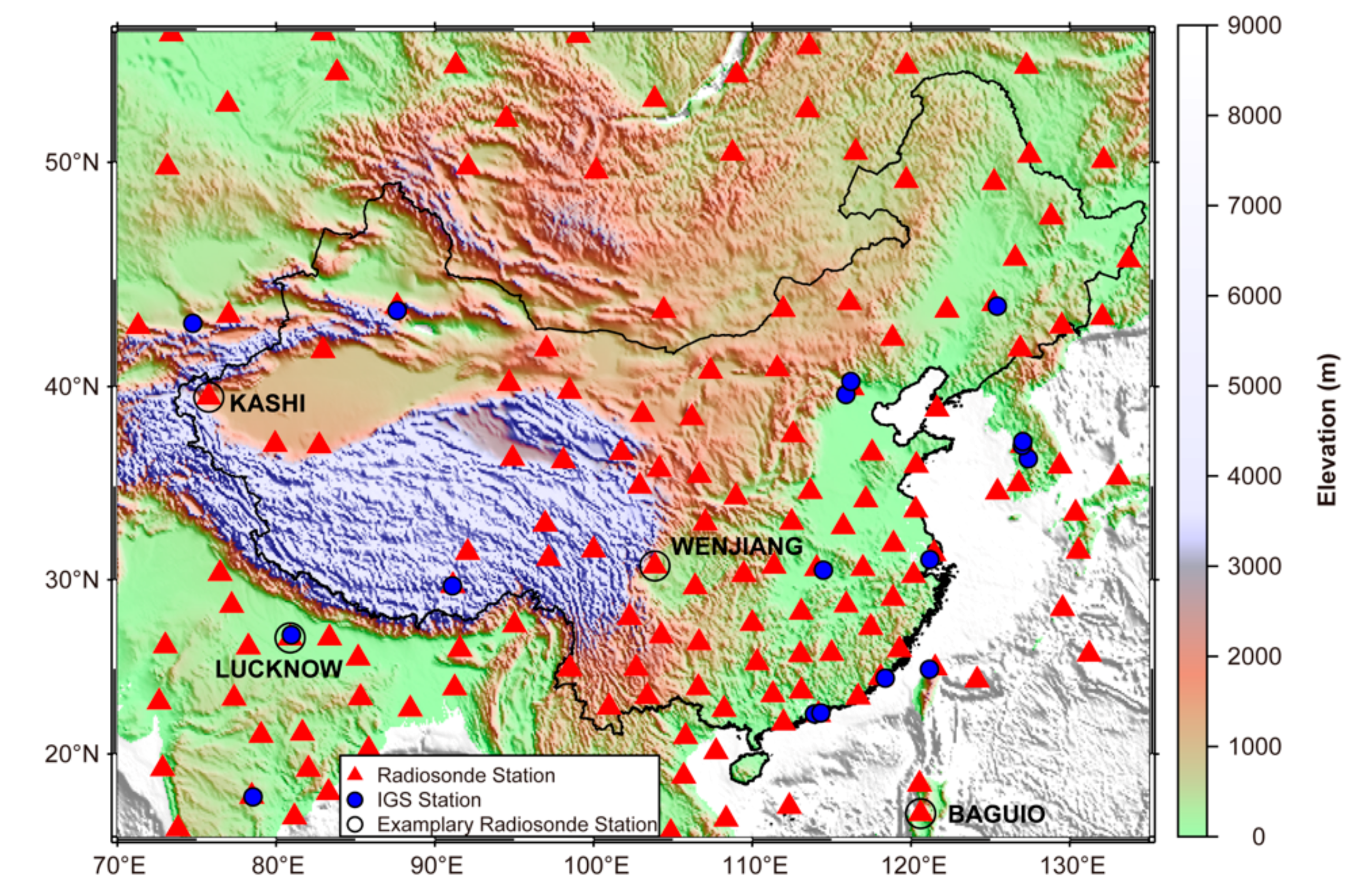
2.1. Data Description

The research area is 15° N to 55° N and 70° E to 135° E, covering the whole of mainland China and its surrounding areas. The GRAPES_MESO data, radiosonde data, and International GNSS Service (IGS) data in the research area are used to generate tropospheric delay and Tm estimates.

The GRAPES_MESO is a new generation of numerical weather forecast system for mesoscale weather prediction developed by the China Meteorological Administration, which covers the period from 29 December 2015 to the present [42]. The GRAPES_MESO assimilates GNSS PWV, FY-2E Cloud-Derived Wind, Constellation Observation System for Meteorology Ionosphere and Climate (COSMIC) data, ground-based radar observations, etc. The GRAPES_MESO forecast profiles have a horizontal resolution of 0.1° × 0.1°, a vertical resolution of 8 levels from 1000 hPa to 100 hPa, and a temporal resolution of 3 h. There are 261,051 grid points in the research area and all available vertical profiles at these points are used. The forecast dataset is provided at 00:00 UTC and 12:00 UTC daily for the coming 72 h (with an interval of 3 h). Meteorological profiles of pressure, temperature, water vapor pressure, and geopotential height in 2017 are used to calculate ZHD, ZWD, and Tm in this study.

Integrated Global Radiosonde Archive (IGRA) launches radiosonde twice daily at 00:00 UTC and 12:00 UTC from 1958 to present, which means the temporal resolution of the radiosonde is 12 h. The radiosonde carries sensors to measure profiles of temperature, humidity, wind speed, etc. Radiosonde profiles are accurate and important data for evaluating other observations or model estimates. Radiosonde profiles often have a height resolution of 21 levels from 1000 hPa or surface pressure in hPa to 1 hPa. Radiosonde profiles of pressure, temperature, relative humidity, and geopotential height at 146 IGRA stations in 2017 are employed to compute ZHD, ZWD, and Tm for the purpose of validation.

GNSS ZTD data at 17 IGS stations in the research area are used to validate the tropospheric delay estimates. Figure 2 gives the topography of the research area as well as the used radiosonde stations and GNSS stations.

2.2. Retrieval of ZHD, ZWD, and Tm Using GRAPES_MESO and Radiosonde Data

To start with, we use stratified pressure, temperature, and relative humidity profiles provided by radiosonde data to calculate water vapor pressure according to [43]. The top pressure level (100 hPa) of GRAPES_MESO and radiosonde data is usually above 16 km, above which almost no water vapor is present. This means that the atmosphere above the top level of the GRAPES_MESO and radiosonde data has no contribution to ZWD or Tm. Therefore, we retrieve the ZWD and Tm using Equations (1)–(3) [3,4] based on only the GRAPES_MESO and radiosonde profiles.

$$ZWD={10}^{-6}{\displaystyle {\int }_h^{\infty }{N}_{w}dh}$$

(1)

$$N_w=k_2\times \frac{e}{T}+k_3\times \frac{e}{T^2}$$

(2)

$$T_m=\frac{{\displaystyle {\int }_h^{\infty }\frac{e}{T}dh}}{{\displaystyle {\int }_h^{\infty }\frac{e}{T^2}dh}}$$

(3)

where $N_w$ indicates wet refractivity,$k_2=64.79 \mathrm{K}/\mathrm{hPa}$, $k_3=\mathrm{377,600} {\mathrm{K}}^2/\mathrm{hPa}$, $e$ and $T$ indicate the water vapor pressure (hPa) and the temperature (K) [44].

When computing ZHD, we need to consider the ZHD above the top level since the whole neutral atmosphere contributes to ZHD. Since the Saastamoinen method (Equation (4)) [11] has good accuracy in computing ZHD, we use it to compute the ZHD above the top pressure layer. ZHD below the top level is computed by integrating the hydrostatic refractivity using Equations (5) and (6) [45]. We obtain the complete ZHD by summing the results from Equations (4) and (5).

$$ZH{D}_{\mathrm{top}}=\frac{0.0022767\cdot P_{top}}{1-0.002667\cdot \cos (2\phi )-0.00000028\cdot h_{top}}$$

(4)

where $\phi$ refers to the latitude (radian), $h_{top}$ is the height of the top pressure level (m), and $P_{top}$ is the top pressure level (hPa).

$$ZHD={10}^{-6}{\displaystyle {\int }_h^{\infty }{N}_h\cdot dh}$$

(5)

$$N_h=k_1\times (P-e)/T$$

(6)

where $N_h$ is hydrostatic refractivity, $k_1=77.604K/hPa$, and $P$ represents the atmospheric pressure (hPa) [44].

Using the above method, we calculate the ZHD, ZWD, and Tm at the lowest pressure level from GRAPES_MESO forecast products at 00:00 UTC, 03:00 UTC, 06:00 UTC, 09:00 UTC, 12:00 UTC, 15:00 UTC, 18:00 UTC, and 21:00 UTC in the research area in 2017. The GRAPES_MESO ZHD, ZWD, and Tm (GRAPES product hereafter) have a horizontal resolution of 0.1° × 0.1° and a temporal resolution of 3 h. We also calculate ZHD, ZWD, and Tm based on radiosonde profiles at the 146 stations, and ZTD at 17 GNSS stations.

2.3. Interpolating GRAPES Products to Any Location

Since the GRAPES products are provided at regular grid nodes, we need to do interpolation to obtain ZHD, ZWD, and Tm at any location and height. The interpolation includes vertical and horizontal interpolation. As for horizontal interpolation, we use a bilinear interpolation method to interpolate interested parameters to the interested location from the nearest four grid nodes. As for vertical interpolation, we adopt the Gaussian function (Equation (7)) to do height correction for ZHD and ZWD [46] and the second-order Fourier function (Equation (8)) for Tm height correction [47] since they have desirable performance by far.

$$T{D}_t=T{D}_0\cdot \exp \left\{\frac{{(h_0-b)}^2-{(h_t-b)}^2}{c^2}\right\}$$

(7)

$$\begin{array}{l}T{m}_t=T{m}_0+a_1\cdot (\cos (w\times h_0)-\cos (w\times h_t))+b_1\cdot (\sin (w\times h_0)-\sin (w\times h_t))\\ +a_2\cdot (\cos (2\times w\times h_0)-\cos (2\times w\times h_t))+b_2\cdot (\sin (2\times w\times h_0)-\sin (2\times w\times h_t))\end{array}$$

(8)

where $T{D}_t$ represents the ZHD or ZWD at target height $h_t$, $T{D}_0$ is the ZHD or ZWD at grid point height $h_0$, $b$ and $c$ are the Gaussian coefficients to be solved by fitting the TD profiles to Equation (7); $T{m}_t$ represents the $Tm$ at target height $h_t$, $T{m}_0$ is the $Tm$ at grid point height, $a_1$, $b_1$, $a_2$, $b_2$, and $w$ are the second-order Fourier coefficients to be deduced by fitting Tm profiles to Equation (8).

We use the solved coefficients of Equations (7) and (8) to correct the ZHD, ZWD, and Tm of GRAPES to the heights of the radiosonde profile. Then, we interpolate the corrected ZHD, ZWD, and Tm to the vertical direction of the site through bilinear interpolation. Figure 3 shows an example of interpolated GRAPES product in the vertical direction at a station (38.47° N, 106.20° E) at 12:00 UTC on 14 January 2017. It can be seen from Figure 3 that the GRAPES ZHD performs the best agreement with the reference data. GRAPES Tm does slightly worse, while GRAPES ZWD exhibits the worst performance. This may be possibly because ZWD/Tm is difficult to calculate accurately due to the high spatiotemporal variation in water vapor. Given the relatively poor accuracy of calculating ZWD/Tm, we propose a further analysis of the GRAPES ZWD and Tm.

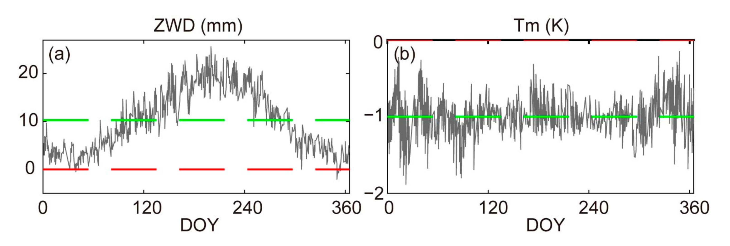
3. Biases in ZWD and Tm

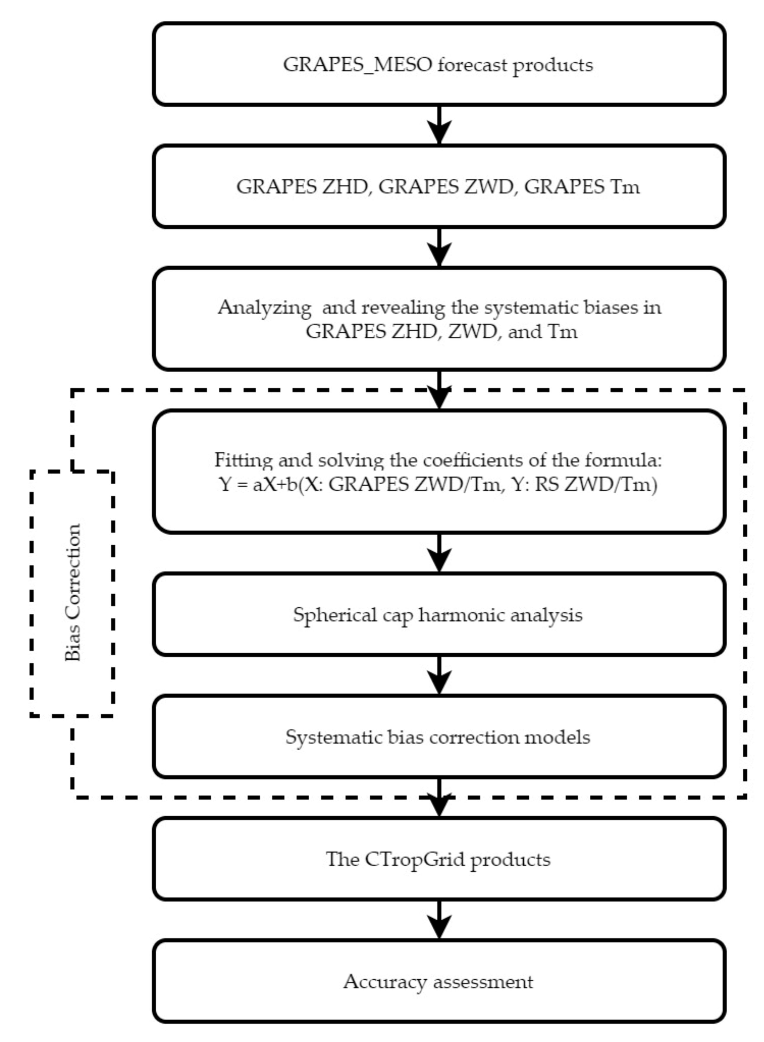
Since the radiosonde based ZHD, ZWD, and Tm have reliable accuracy and are usually used to assess other estimates [37,43,48,49,50], we take the radiosonde based ZHD, ZWD, and Tm as the reference values to validate the GRAPES ZHD, ZWD, and Tm in 2017. After interpolating the GRAPES ZHD, ZWD, and Tm from the coming 00:00 UTC and 12:00 UTC to the 146 radiosonde stations using the methods described in Section 2.2, we first calculate the mean bias, STD, and RMS of the site-specific of the differences between GRAPES-based and radiosonde-based ZHD, ZWD, and Tm (GRAPES products minus radiosonde products). Then, we average all the mean bias, STD, and RMS of the sites-specific to get the station mean bias, standard deviation (STD), and RMS. Three times standard deviation is used as a criterion to remove outliers. Statistical results demonstrates that GRAPES ZWD has a bias of 10.5 mm and Tm has a bias of −1.0 K, which are very large biases given the RMSs of ZWD and Tm are only 25.5 mm and 1.9 K. While GRAPES ZHD has a very small bias, only 1.5 mm, considering the RMS is 8.9 mm. Besides, the STD of GRAPES ZHD, ZWD, and Tm is 5.2 mm, 21.2 mm, and 1.5 K, respectively. To investigate the biases in ZWD and Tm, we calculate daily biases (spatial average of differences between GRAPES ZWD (Tm) and radiosonde ZWD (Tm) in the same day) and show them in Figure 4. We also calculate the temporal average of differences at the same station to obtain the spatial variations of biases, which is shown in Figure 5.

Figure 4a displays that the GRAPES ZWD has positive biases nearly every day of 2017 and its bias has clear seasonal pattern, i.e., greater in summer and smaller in winter, fluctuating around 10 mm. It means that the GRAPES ZWD tends to be larger than the radiosonde ZWD. Figure 4b presents that the GRAPES Tm has negative biases in the whole 2017 ranging between −1.5–−0.5 K, suggesting that the GRAPES Tm is always smaller than the radiosonde Tm. Tm bias does not show any seasonal pattern as the ZWD bias does. These are because the water vapor pressure has a small negative bias (−1.7 hPa), and the temperature has a significant negative bias (−8.9 K) (see Figure A1 in Appendix A). Moreover, Figure 5 reveals that the biases in GRAPES ZWD and Tm are not even in space. Therefore, we need to correct the system biases in GRAPES ZWD and Tm before we use them. We prefer to make corrections directly to ZWD and Tm rather than to the meteorological data since the latter are stratified data which means we need to correct them layer by layer.

4. Bias Correction

4.1. Correcting Systematic Biases between GRAPES-Based and Radiosonde-Based ZWD(Tm)

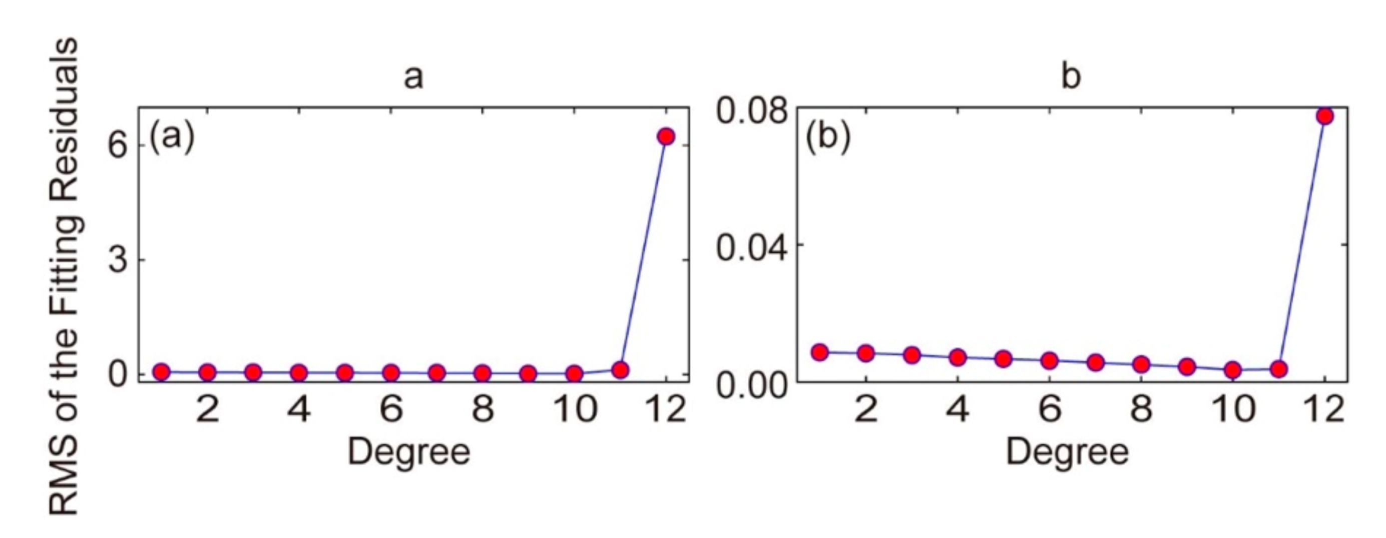
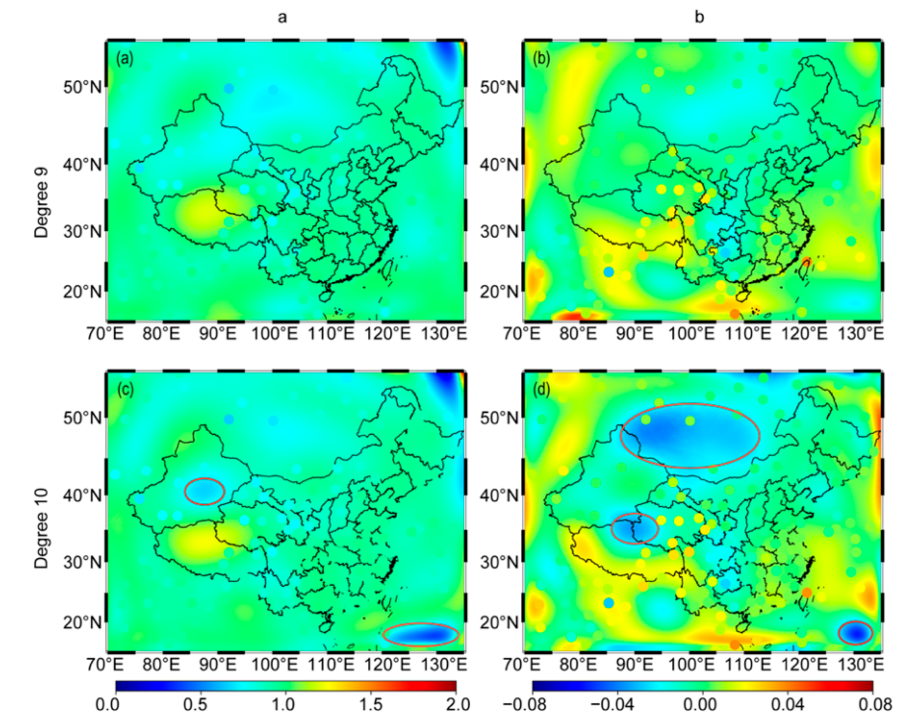
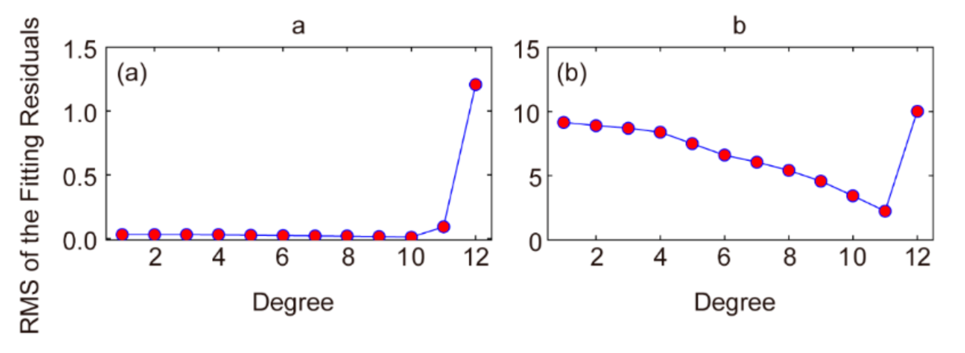
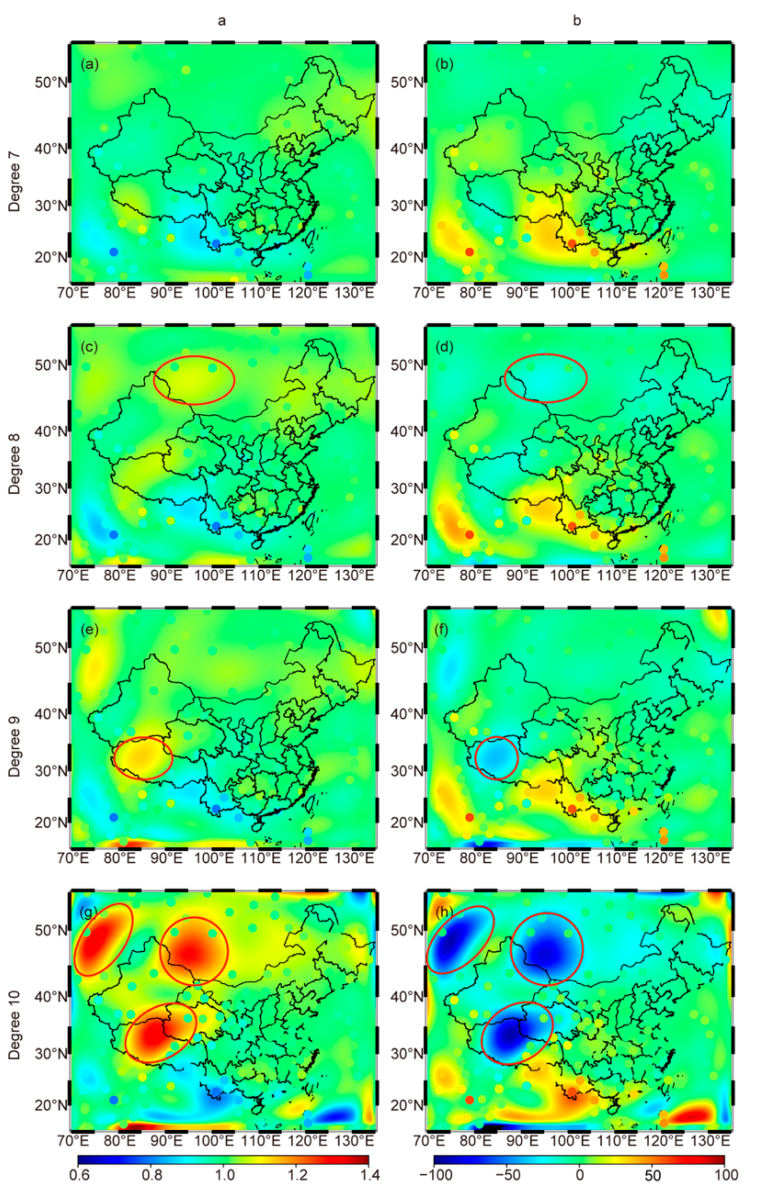
A linear model has been used to describe the systematic bias between two datasets in [51] and has also been used to calibrate the tropospheric products provided by the Technische Universität Wien [52]. This method is expressed as Equation (9) in which $Y$ is the reference value and $X$ is the value to be calibrated. Parameters $a$ and $b$ are used to quantify the proportional bias and constant bias. In this study, we treat radiosonde ZWD (Tm) as the reference values and use them to calibrate the GRAPES ZWD (Tm).

$$Y=a\cdot X+b$$

(9)

We first interpolate GRAPES ZWD and Tm to the 146 radiosonde stations at 00:00 UTC and 12:00 UTC, thereby forming GRAPES-radiosonde ZWD (Tm) pairs, which are then used to fit and solve Equation (9) for $a$ and $b$ yearly using the method of least squares. We do not change them with time until we re-estimate them. We also perform the t-Test [53] on the estimates of $a$ and $b$ to check their statistical significance. The results in Figure A2 show that 100%, 70.0%, 100%, and 62.3% of the stations have $p$ values smaller than 0.05 for $ZWD-a$, $ZWD-b$, $Tm-a$, and $Tm-b$. This demonstrates the estimated $a$ and $b$ are statistically significant overall. After calibration, the biases of GRAPES ZWD and Tm are close to zero. Figure 6 shows examples of ZWD and Tm time series before and after calibration in comparison with the radiosonde result at BAGUIO, WENJIANG, LUCKNOW, and KASHI stations (see Figure 2) in 2017. Figure 6a,c,e,g show that the calibrated GRAPES ZWD agrees better with the radiosonde ZWD after calibration. Figure 6b,d,f,h demonstrate that the calibrated GRAPES Tm has a better agreement with the radiosonde Tm than the GRAPES Tm. After calibration, the ZWD and Tm biases are largely mitigated and even eliminated. These suggest clearly that Equation (9) is effective in calibrating the biases in GRAPES ZWD and Tm.

4.2. Interpolating $a$ and $b$ Using a Spherical Cap Harmonic (SCH) Model

To convert the systematic biases correction to any location of GRAPES data (from point to surface), we propose to use spherical cap harmonic (SCH) functions to fit $a$ and $b$ over all of China using the $a$ and $b$ at 146 radiosonde stations obtained in Section 4.1, then establish some SCH models for systematic bias correction. The SCH analysis has been used to represent the geomagnetic fields [54,55,56], the regional gravity fields [57,58], the ionospheric total electron content [59,60], the sea level [61], and the PWV fields [62], etc. In this study, we use a SCH model to represent the fields of systematic bias embodied by $a$ and $b$. The expression of the SCH model is as follows:

$$C={\displaystyle {\sum }_{k=0}^N{\displaystyle {\sum }_{m=0}^k{a}_e{(\frac{a_e}{r})}^{n_k(m)+1}{P}_{n_k(m)}^m(\cos \theta )\cdot \{g_k^m\cos (m\lambda )+h_k^m\sin (m\lambda )\}}}$$

(10)

where, $C$ represents $a$ or $b$. $a_e$ is the radius of the earth, which is set as 6,378,137 m.$r,\theta ,\lambda$ refer to the radial distance, the colatitude, and the longitude of a point in the spherical cap coordinate system. $P_{n_k(m)}^m$ is the associated Legendre function. $n_k(m)$ and $m$ denote the degree and order of the SCH model, respectively. $N$ represents the maximum degree of the expansion for $a$ or $b$. $g_k^m$ and $h_k^m$ are the coefficients of the spherical cap harmonic expansion to be determined.

In this study, the $n_k(m)$ and $P_{n_k(m)}^m$ are determined based on the methods presented in [62]. When we feed $a$ ($b$), $P_{n_k(m)}^m$ and spherical cap coordinates into Equation (10), we obtain linear equations in which $g_k^m$ and $h_k^m$ are coefficients to be determined. We use a least-square method to solve these linear equations.

To ensure the reliability of the SCH models, only the reliable $a$ ($b$) sets are used. The reliable $a$ ($b$) is identified by two criteria: $i$. the GRAPES data and radiosonde data used to calculate $a$ ($b$) must have a correlation coefficient greater than 0.8; $ii$. among the calculated $a$ ($b$) sets, reliable $a$ ($b$) should be within the triple STD of $a$ ($b$). Moreover, to avoid edge effects, we add some virtual stations outside mainland China, at which $a$ and $b$ are set to 1 and 0.

To determine the best degree and order for the SCH model, we fit the SCH model with degrees that increase from 0 to 12. Note that the maximum order always equals the maximum degree in this work. We fit $a$ and $b$ for ZWD (Tm) using the SCH models with increasing degrees, and we calculate the misfit RMS, which is then used to assess the fitting accuracy. Figure 7 shows the misfit RMS of $a$ and $b$ versus degrees of the SCH model for ZWD. It demonstrates that the misfit RMS of $a$ keeps small when the degree increases from 1 to 10 but sharply increases after degree 10. Figure 7b shows that the misfit RMS of $b$ decreases when the degree increases from 1 to 11 but sharply increases after degree 11. This suggests degree 10 or 11 may be optimal for $a$ and $b$. Figure 8 shows the fitting map of $a$ and $b$, in which Figure 6d and Figure 8c exhibit some distortions (marked by red ellipses). This indicates we overfitted $a$ and $b$. When we set the degree to 9, the main distortions disappeared. Therefore, to balance the fitting accuracy and the number of distortions, we use degree 9 to fit $a$ and $b$ for ZWD. The misfit RMS of $a$ and $b$ versus degrees (see Figure 9) and the fitting map (see Figure 10) of the SCH model for Tm have a similar phenomenon to that for ZWD. Thus, we employ degree 7 to fit $a$ and $b$ for Tm.

When the degrees are determined, we solve the SCH models by computing $g_k^m$ and $h_k^m$ for $a$ and $b$ of ZWD and Tm. We then use the obtained SCH models to interpolate $a$ and $b$ to each GRAPES grid point with a high spatial resolution (0.1° × 0.1°), by which we correct the GRAPES ZWD and Tm over all of China. The corrected gridded ZWD and Tm together with the ZHD are provided online and named CTropGrid product. When using CTropGrid product, users need to do spatial and temporal interpolation. For spatial interpolation, the vertical interpolation and horizontal interpolation methods in Section 2.3 are recommended, and height correction parameters are provided with the CTropGrid products. For temporal interpolation, a cubic spline interpolation [39] is advised.

5. Results

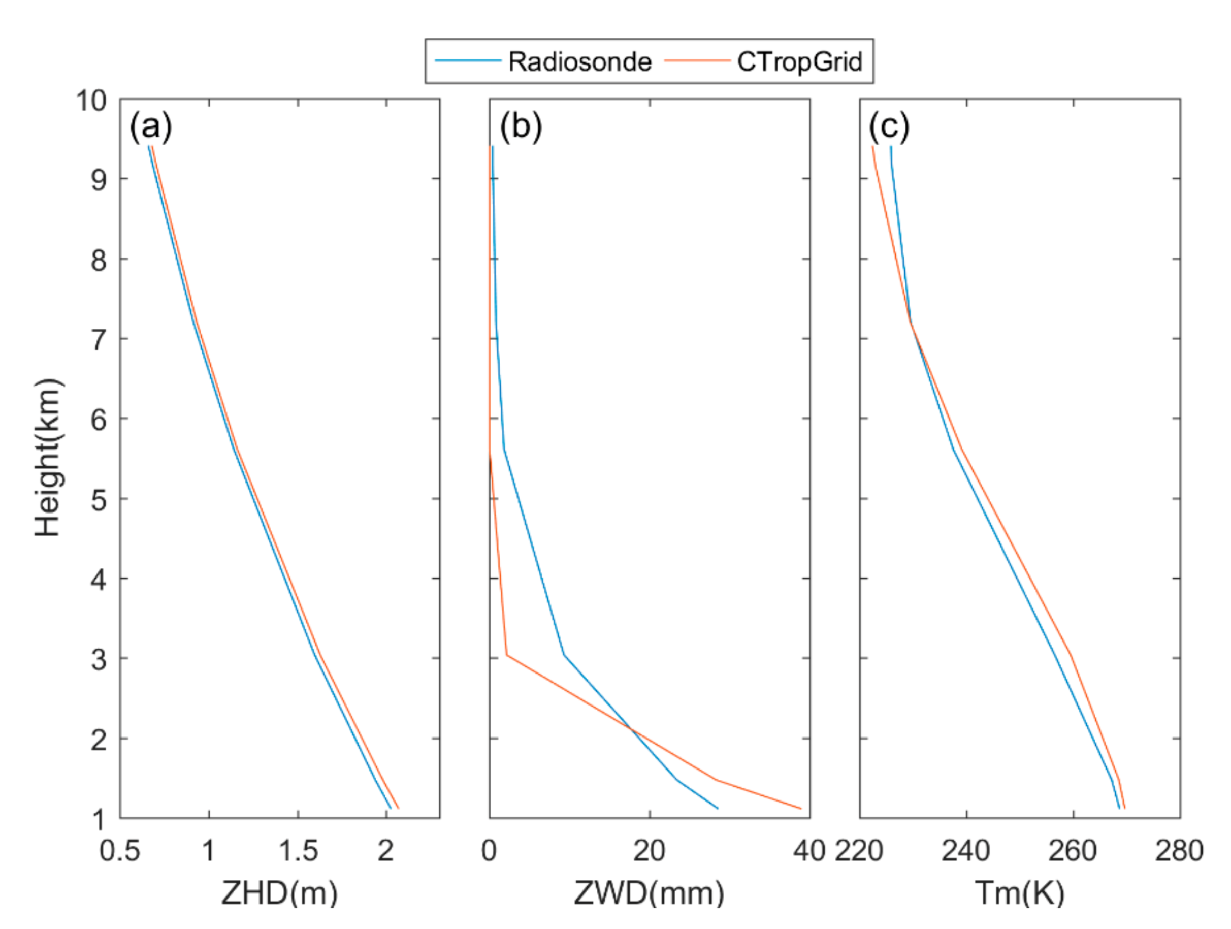
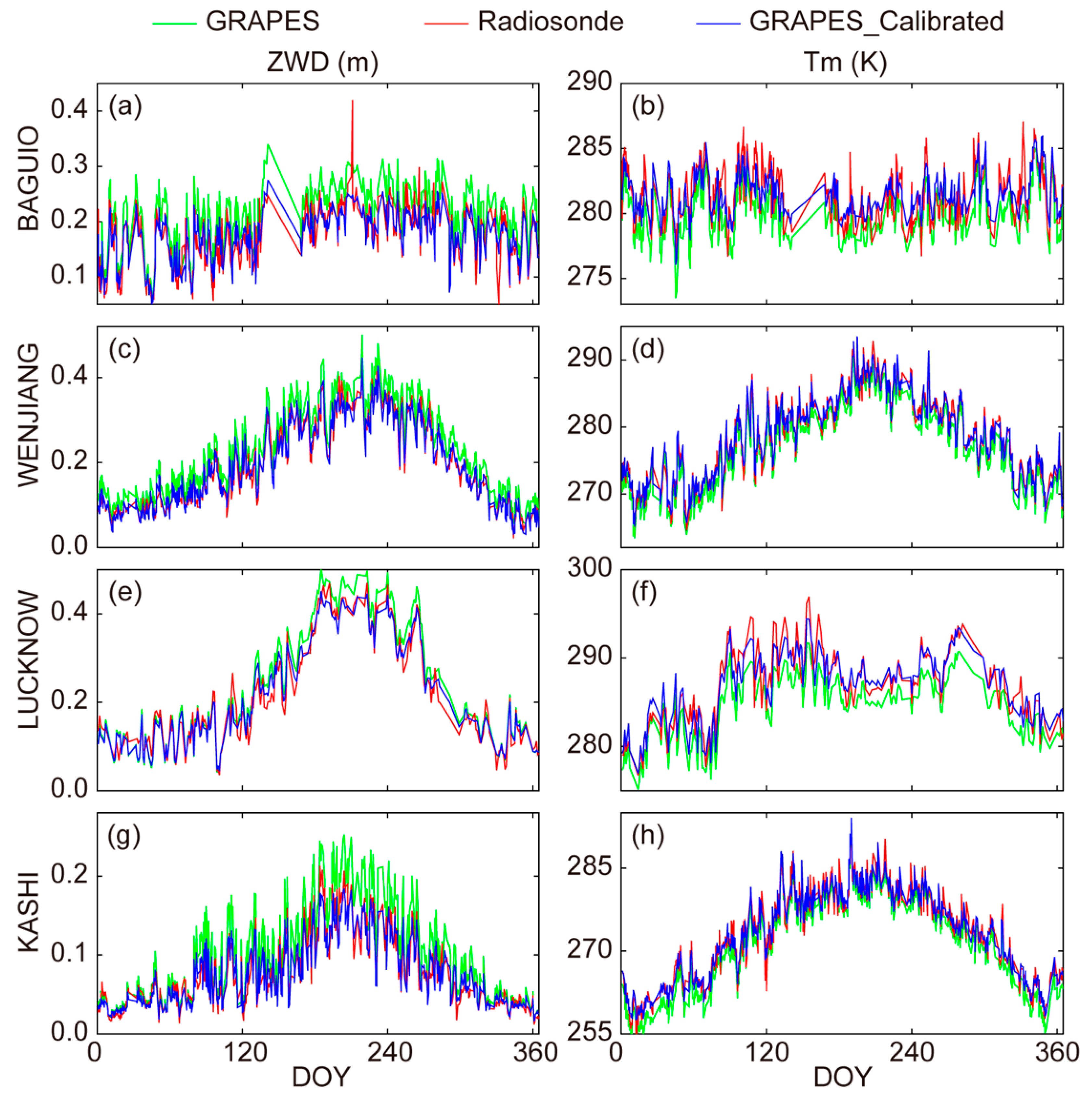
5.1. Validation with Radiosonde Data

5.1.1. Overall Performance

ZHD, ZWD, and Tm derived from radiosonde data at 146 stations in 2017 are employed to validate the CTropGrid ZHD, ZWD, and Tm in comparison with the GPT2w model (1° version).

Table 1. Statistics of the mean bias, STD, and RMS for ZHD, ZWD, and Tm derived from the CTropGrid and the GPT2w model at radiosonde stations in the year 2017. The numbers in the square brackets indicate the range of bias, STD, or RMS.

Method	ZHD (mm)			ZWD (mm)			Tm (K)
	Bias	STD	RMS	Bias	STD	RMS	Bias	STD	RMS
CTropGrid	1.5	5.2	8.9	−0.7	19.0	20.2	−0.1	1.5	1.5
	[−15.8, 35.8]	[0.7, 7.3]	[3.0, 35.9]	[−24.1, 26.2]	[7.9, 38.3]	[10.2, 38.7]	[−2.2, 1.3]	[0.7, 2.5]	[0.7, 2.6]
GPT2w	0.6	9.3	10.1	−7.0	43.8	45.5	−0.7	3.5	3.8
	[−4.0, 45.4]	[4.0, 21.0]	[4.4, 45.8]	[−61.8, 20.5]	[13.8, 78.1]	[13.8, 79.0]	[−7.1, 3.8]	[1.4, 5.7]	[1.4, 7.7]

presents the accuracy information quantified by bias, STD, and RMS. Comparing the statistical results in Section 3 and Table 1, the CTropGrid ZWD and Tm have much smaller biases than the GRAPES ones (−0.7 mm vs. 10.5 mm for ZWD, −0.1 K vs. −1.0 K for Tm), indicating the bias correction method effectively mitigates the bias in ZWD and Tm. Due to this, the RMS is also improved (20.2 mm vs. 25.5 mm for ZWD and 1.5 K vs. 1.9 K for Tm).

Table 1 also shows that the CTropGrid ZHD has a slightly larger bias than that of the GPT2w model (1.5 mm vs. 0.6 mm) but a much smaller mean STD (5.2 mm vs. 9.3 mm) and RMS (8.9 mm vs. 10.1 mm). The total improvements measured by RMS are 11.9%. The CTropGrid ZWD and Tm have much smaller biases than the GPT2w ones (−0.7 mm vs. −7.0 mm for ZWD, −0.1 K vs. −0.7 K for Tm), and the improvements exceed 90.0% for ZWD and 85.8% for Tm. Moreover, the CTropGrid ZWD and Tm have better STD and RMS than the GPT2w ZWD and Tm. The CTropGrid ZWD improves the total accuracy by 55.6% compared to the GPT2w model measured by RMS. The CTropGrid Tm has an accuracy improvement of 60.5% in terms of RMS against the GPT2w model. Overall, all the CTropGrid products exhibit apparent superiority to the GPT2w model in estimating ZHD, ZWD, and Tm.

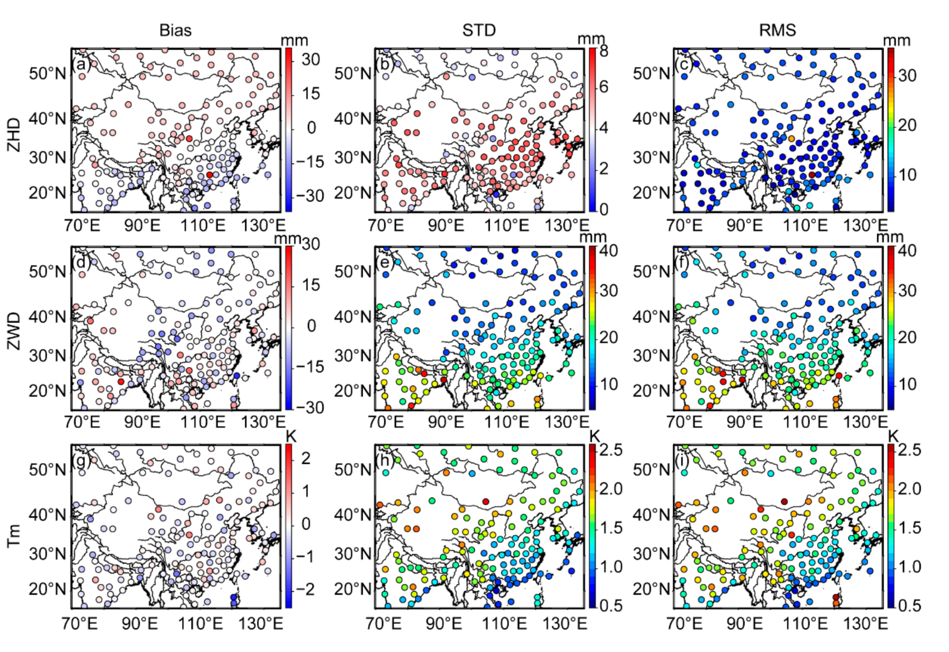
5.1.2. Spatial Variations of Accuracy

To analyze the spatial variations of the accuracy of the CTropGrid products, the mean bias, STD, and RMS of ZHD, ZWD, and Tm are computed at the 146 radiosonde sites and shown in Figure 11. Figure 11a shows that the CTropGrid ZHD has almost the same amount of positive and negative bias, and the positive bias tends to appear at middle- and high-latitude regions while the negative bias mainly appears at the low-latitude regions. Figure 11b,c present that both STD and RMS of the CTropGrid ZHD are uniformly distributed overall, demonstrating that the accuracy of the CTropGrid ZHD has spatially even accuracy in the study area.

After calibration, the biases of the CTropGrid ZWD and Tm are small and evenly distributed (Figure 11d,g), indicating that the proposed calibration method eliminates the spatially varying biases. Figure 11e,f show that the STD and RMS of the CTropGrid ZWD have similar spatial patterns, i.e., larger at low latitudes and smaller at middle and high latitudes. This is attributed to that the water vapor at low latitudes is richer and changes more rapidly than at high latitudes, which causes more uncertainties in ZWD modeling. Even so, the largest RMS is still below 40 mm.

Figure 11h,i demonstrates that the STD and RMS of CTropGrid Tm also have similar spatial patterns, i.e., overall larger in the northwest and smaller in the southeast, but all the RMSs are below 3.0 K. The above results overall imply that the CTropGrid products have satisfactory accuracy in the whole research area.

Figure 12 presents the percentage RMS reductions of the CTropGrid products relative to the GPT2w model. Positive values mean RMS is decreased while negative values mean RMS is increased. It shows that the RMS of the CTropGrid ZHD is reduced at 93 stations but increased at 53 stations in the very southern regions. The RMS of the CTropGrid ZWD is reduced at almost all the stations except for a few in the Qinghai–Tibetan Plateau. The mean RMS reduction of CTropGrid ZWD reaches up to 51.7%. The RMS is mostly reduced in eastern China and less reduced in western China. The RMS of the CTropGrid Tm is reduced at all stations with a percentage reduction of 57.7% in average. Similar to ZWD, the largest RMS reduction appears in eastern China and less reduction in western China. These further demonstrate that the CTropGrid products have better accuracy and spatial representation for describing ZHD, ZWD, and Tm than the GPT2w model in the research area.

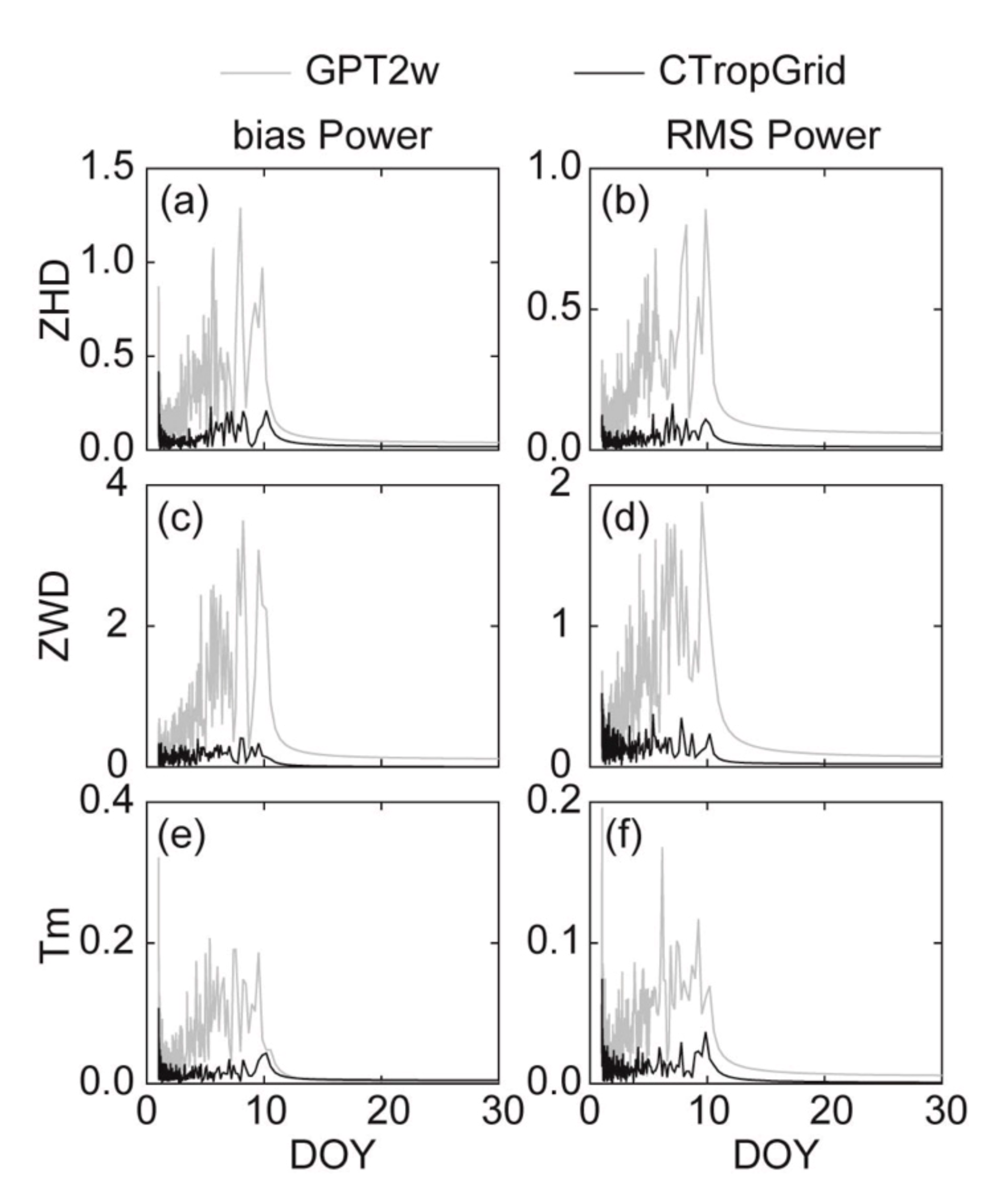
5.1.3. Temporal Variations of Accuracy

We calculate the spatially averaged bias and RMS of the CTropGrid products and the GPT2w model output daily to understand the temporal variations of the data accuracy. The results are shown in Figure 13. Figure 13a,b manifest that the bias and RMS of the CTropGrid ZHD exhibit much smaller temporal variations than the GPT2w results. The biases are closer to zero, and the RMS is much smaller than the GPT2w results. The above indicate again that the CTropGrid provides better ZHD products than the GPT2w model and mitigate the temporal variations of the accuracy. Figure 13c,d show that the CTropGrid ZWD has much smaller daily bias (around zero) and RMS (around 20 mm) than the GPT2w model and the improvement is very apparent. In addition, the seasonal variation in ZWD bias (Figure 4) is greatly weakened due to the systematic bias correction. Similar improvements can also be observed in Tm (Figure 13e,f). The above results suggest that the accuracy of the CTropGrid products is very stable in time and thus further verifies their superiority in computing ZHD, ZWD, and Tm.

To investigate how the accuracy is improved, a fast Fourier transform (FFT) analysis is performed on the daily bias and RMS. Before applying FFT, we use a high-pass filter to remove the signals whose frequency is lower than half month. Then, we focus on analyzing the synoptic-scale signals. Figure 14 shows the power spectrums of the bias and RMS from the GPT2w model and from the CTropGrid products. It is observed that both the bias and RMS of ZHD, ZWD, and Tm from the GPT2w model have strong power at time scales of a few days (1–10 days), which is attributed to the unmodeled synoptic variations. In contrast, the bias and RMS of the three parameters from the CTropGrid products have much weaker power at the same timescales than the GPT2w model, indicating the CTropGrid products well model the synoptic variations in ZHD, ZWD, and Tm. This is also reflected in Figure 13 where the TropGrid products’ uncertainties show much fewer variations at synoptic timescales than the GPT2w model. This is another main advancement of the CTropGrid products than the GPT2w model.

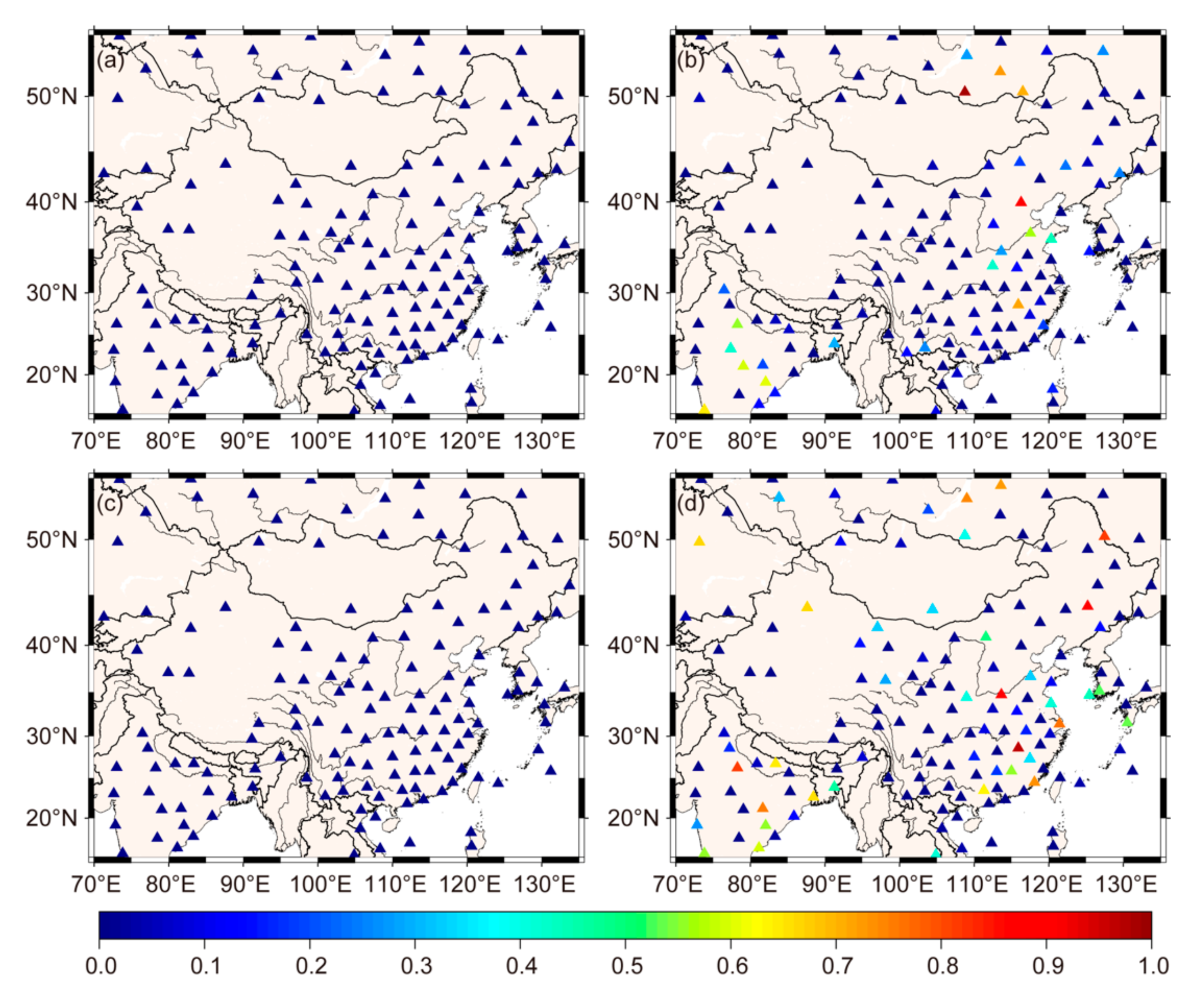
5.2. Validate the CTropGrid Products with IGS ZTD

We employ the IGS ZTD data to validate the CTropGrid ZTD. IGS ZTD estimates are produced through Bernese GPS Software 5.0 using the precise point positioning (PPP) method [63]. IGS Final satellite orbit and clock products are used to determine the position of the satellites and time [63]. Niell model [64] and GMF mapping functions [65] are used to provide a priori tropospheric delay. The IGS ZTD has a specified accuracy of 4 mm, which is commonly used to validate other observations and model ZTD [5,9,22,33,38]. The CTropGrid ZTD is obtained by summing the ZHD and the ZWD. For comparison, we interpolate the CTropGrid ZTD to the epoch of the IGS ZTD using the cubic spline interpolation method [39]. For each IGS site, the bias, STD, and RMS of the differences between IGS ZTD and the CTropGrid ZTD are calculated in 2017. The same processing is also applied to the GPT2w ZTD. The statistical results are displayed in

Table 2. Statistics of bias, STD, and RMS for ZTD from the CTropGrid product and the GPT2w model at IGS stations in the year 2017.

Model	Bias (mm)	STD (mm)	RMS (mm)
GPT2w	1.0 [−13.9, 21.8]	45.2 [17.5, 67.0]	46.3 [20.9, 67.2]
CTropGrid	−0.7 [−16.8, 23.6]	34.1 [22.7, 49.6]	35.8 [24.7, 49.8]

. It shows that the absolute bias of the CTropGrid ZTD is slightly improved compared to that of the GPT2w model (0.7 mm vs. 1.0 mm). The STD of the CTropGrid ZTD is 11.1 mm (24.6%) smaller than that of the GPT2w model, and the site-dependent STDs also have a smaller range (22.7–49.6 mm vs. 17.5–67.0 mm). The RMS of the CTropGrid ZTD is 10.5 mm (22.7%) smaller than the GPT2w model, and the range of site-dependent RMSs apparently becomes narrower. All the above demonstrates that the CTropGrid products provide more accurate and stable tropospheric delay than the GPT2w model, and the overall improvement reaches 22.7% in terms of RMS.

To further analyze the temporal variations of the CTropGrid ZTD’s accuracy, we also calculate the spatially averaged bias and RMS of the CTropGrid and the GPT2w ZTD twice daily and show them in Figure 15. As observed in Figure 15, during the year 2017, most of the biases and RMSs of the CTropGrid ZTD are smaller than that of the GPT2w ZTD. In addition, the bias and RMS of ZTD from the CTropGrid products have weaker sub-daily and seasonal variations than the GPT2w model. These indicate that the CTropGrid products are more accurate and stable than the GPT2w model for forecasting ZTD.

6. Conclusions

We yield the zenith hydrostatic/wet delay and weighted mean temperature products based on GRAPES_MESO forecasting products in China but found systematic biases in ZWD and Tm. We then use a linear model and a spherical cap harmonic model to calibrate the biases. Finally, we provide calibrated ZHD, ZWD, and Tm products at 0.1° grid nodes with a temporal resolution of 3 h and term them the “CTropGrid” products.

Validated by the radiosonde data, the CTropGrid products improve the total accuracy of ZHD by 11.9% in terms of RMS compared to the GPT2w model. The improvements become 55.6% and 60.5% for the ZWD and Tm. The CTropGrid products also greatly reduced the biases for ZWD and Tm, the reductions are as high as 90.0% and 85.8%. Validated by the IGS ZTD data, the absolute bias and RMS of the ZTD from the CTropGrid are 30% and 22.7% smaller than that of the GPT2w model. All these results verify that the CTropGrid products are more accurate and stable than the GPT2w model in estimating tropospheric delay and Tm. This great improvement is attributed to the well modeling of the synoptic variations in the three parameters, which cannot be modeled by the empirical models.

Since the CTropGrid products can provide better forecasted tropospheric delay and Tm products than the empirical models, it will be a very useful dataset for real-time GNSS applications and GNSS meteorology. Due to this, the CTropGrid products are a meaningful contribution to the GNSS community.

References

1. Chen, Q.; Song, S.; Heise, S.; Liou, Y.-A.; Zhu, W.; Zhao, J. Assessment of ZTD derived from ECMWF/NCEP data with GPS ZTD over China. GPS Solut. 2011, 15, 415–425. [Google Scholar] [CrossRef]
2. Jin, S.; Park, J.-U.; Cho, J.-H.; Park, P.-H. Seasonal variability of GPS-derived zenith tropospheric delay (1994–2006) and climate implications. J. Geophys. Res. 2007, 112, D09110. [Google Scholar] [CrossRef]
3. Davis, J.L.; Herring, T.A.; Shapiro, I.I.; Rogers, A.E.E.; Elgered, G. Geodesy by radio interferometry: Effects of atmospheric modeling errors on estimates of baseline length. Radio Sci. 1985, 20, 1593–1607. [Google Scholar] [CrossRef]
4. Bevis, M.; Businger, S.; Herring, T.A.; Rocken, C.; Anthes, R.A.; Ware, R.H. GPS meteorology: Remote sensing of atmospheric water vapor using the global positioning system. J. Geophys. Res. Atmos. 1992, 97, 15787–15801. [Google Scholar] [CrossRef]
5. Li, W.; Yuan, Y.; Ou, J.; Chai, Y.; Li, Z.; Liou, Y.-A.; Wang, N. New versions of the BDS/GNSS zenith tropospheric delay model IGGtrop. J. Geod. 2014, 89, 73–80. [Google Scholar] [CrossRef]
6. Askne, J.; Nordius, H. Estimation of tropospheric delay for microwaves from surface weather data. Radio Sci. 1987, 22, 379–386. [Google Scholar] [CrossRef]
7. Tregoning, P.; Herring, T.A. Impact of a priori zenith hydrostatic delay errors on GPS estimates of station heights and zenith total delays. Geophys. Res. Lett. 2006, 33. [Google Scholar] [CrossRef] [Green Version]
8. Wang, X.M.; Zhang, K.F.; Wu, S.Q.; Fan, S.J.; Cheng, Y.Y. Water vapor-weighted mean temperature and its impact on the determination of precipitable water vapor and its linear trend. J. Geophys. Res. Atmos. 2016, 121, 833–852. [Google Scholar] [CrossRef]
9. Chen, P.; Ma, Y.; Liu, H.; Zheng, N. A New Global Tropospheric Delay Model Considering the Spatiotemporal Variation Characteristics of ZTD with Altitude Coefficient. Earth Space Sci. 2020, 7, e2019EA000888. [Google Scholar] [CrossRef]
10. Li, S.; Xu, T.; Jiang, N.; Yang, H.; Wang, S.; Zhang, Z. Regional Zenith Tropospheric Delay Modeling Based on Least Squares Support Vector Machine Using GNSS and ERA5 Data. Remote Sens. 2021, 13, 1004. [Google Scholar] [CrossRef]
11. Saastamoinen, J.H. Atmospheric Correction for the Troposphere and the Stratosphere in Radio Ranging Satellites. Use Artif. Satell. Geod. 1972, 15, 247–251. [Google Scholar] [CrossRef]
12. Hopfield, H.S. Two-quartic tropospheric refractivity profile for correcting satellite data. J. Geophys. Res. 1969, 74, 4487–4499. [Google Scholar] [CrossRef]
13. Collins, J.P.; Langley, R.B. A Tropospheric Delay Model for the User of the Wide Area Augmentation System; Department of Geodesy and Geomatics Engineering, University of New Brunswick: Fredericton, NB, Canada, 1997. [Google Scholar]
14. Bohm, J.; Moller, G.; Schindelegger, M.; Pain, G.; Weber, R. Development of an improved empirical model for slant delays in the troposphere (GPT2w). GPS Solut. 2015, 19, 433–441. [Google Scholar] [CrossRef] [Green Version]
15. Lagler, K.; Schindelegger, M.; Bohm, J.; Krasna, H.; Nilsson, T. GPT2: Empirical slant delay model for radio space geodetic techniques. Geophys. Res. Lett. 2013, 40, 1069–1073. [Google Scholar] [CrossRef] [Green Version]
16. Landskron, D.; Böhm, J. VMF3/GPT3: Refined discrete and empirical troposphere mapping functions. J. Geod. 2017, 92, 349–360. [Google Scholar] [CrossRef] [PubMed]
17. Boehm, J.; Kouba, J.; Schuh, H. Forecast Vienna Mapping Functions 1 for real-time analysis of space geodetic observations. J. Geod. 2008, 83, 397–401. [Google Scholar] [CrossRef]
18. Krueger, E.; Schüler, T.; Arbesser-Rastburg, B. The standard tropospheric correction model for the European satellite navigation system Galileo. In Proceedings of the XXVIIIth general assembly of International Union of Radio Science (URSI), New Delhi, India, 23–29 October 2005. [Google Scholar]
19. Schuler, T. The TropGrid2 standard tropospheric correction model. GPS Solut. 2014, 18, 123–131. [Google Scholar] [CrossRef]
20. Penna, N.; Dodson, A.; Chen, W. Assessment of EGNOS tropospheric correction model. J. Navig. 2001, 54, 37–55. [Google Scholar] [CrossRef] [Green Version]
21. Li, J.; Zhang, B.; Yao, Y.; Liu, L.; Sun, Z.; Yan, X. A Refined Regional Model for Estimating Pressure, Temperature, and Water Vapor Pressure for Geodetic Applications in China. Remote Sens. 2020, 12, 1713. [Google Scholar] [CrossRef]
22. Li, W.; Yuan, Y.; Ou, J.; He, Y. IGGtrop_SH and IGGtrop_rH: Two Improved Empirical Tropospheric Delay Models Based on Vertical Reduction Functions. IEEE Trans. Geosci. Remote Sens. 2018, 56, 5276–5288. [Google Scholar] [CrossRef]
23. Yao, Y.; Hu, Y.; Yu, C.; Zhang, B.; Guo, J. An improved global zenith tropospheric delay model GZTD2 considering diurnal variations. Nonlinear Process. Geophys. 2016, 23, 127–136. [Google Scholar] [CrossRef] [Green Version]
24. Yao, Y.; He, C.; Zhang, B.; Xu, C. A new global zenith tropospheric delay model GZTD. Chin. J. Geophys. 2013, 56, 2218–2227. [Google Scholar] [CrossRef]
25. Sun, Z.; Zhang, B.; Yao, Y. An ERA5-Based Model for Estimating Tropospheric Delay and Weighted Mean Temperature Over China With Improved Spatiotemporal Resolutions. Earth Space Sci. 2019, 6, 1926–1941. [Google Scholar] [CrossRef]
26. Sun, J.L.; Wu, Z.L.; Yin, Z.D.; Ma, B. A simplified GNSS tropospheric delay model based on the nonlinear hypothesis. GPS Solut. 2017, 21, 1735–1745. [Google Scholar] [CrossRef]
27. Zhang, H.; Yuan, Y.; Li, W.; Zhang, B.; Ou, J. A grid-based tropospheric product for China using a GNSS network. J. Geod. 2017, 92, 765–777. [Google Scholar] [CrossRef]
28. Chen, B.; Liu, Z. A Comprehensive Evaluation and Analysis of the Performance of Multiple Tropospheric Models in China Region. IEEE Trans. Geosci. Remote Sens. 2016, 54, 663–678. [Google Scholar] [CrossRef]
29. Yao, Y.B.; Zhu, S.; Yue, S.Q. A globally applicable, season-specific model for estimating the weighted mean temperature of the atmosphere. J. Geod. 2012, 86, 1125–1135. [Google Scholar] [CrossRef]
30. Yao, Y.B.; Zhang, B.; Yue, S.Q.; Xu, C.Q.; Peng, W.F. Global empirical model for mapping zenith wet delays onto precipitable water. J. Geod. 2013, 87, 439–448. [Google Scholar] [CrossRef]
31. Yao, Y.B.; Xu, C.Q.; Zhang, B.; Cao, N. GTm-III: A new global empirical model for mapping zenith wet delays onto precipitable water vapour. Geophys. J. Int. 2014, 197, 202–212. [Google Scholar] [CrossRef] [Green Version]
32. Huang, L.; Jiang, W.; Liu, L.; Chen, H.; Ye, S. A new global grid model for the determination of atmospheric weighted mean temperature in GPS precipitable water vapor. J. Geod. 2019, 93, 159–176. [Google Scholar] [CrossRef]
33. Zhang, H.; Yuan, Y.; Li, W.; Ou, J.; Li, Y.; Zhang, B. GPS PPP-derived precipitable water vapor retrieval based on Tm/Ps from multiple sources of meteorological data sets in China. J. Geophys. Res. Atmos. 2017, 122, 4165–4183. [Google Scholar] [CrossRef]
34. Huang, L.; Liu, L.; Chen, H.; Jiang, W. An improved atmospheric weighted mean temperature model and its impact on GNSS precipitable water vapor estimates for China. GPS Solut. 2019, 23, 1–16. [Google Scholar] [CrossRef]
35. Emardson, T.R.; Derks, H.J.P. On the relation between the wet delay and the integrated precipitable water vapour in the European atmosphere. Meteorol. Appl. 2000, 7, 61–68. [Google Scholar] [CrossRef]
36. Yang, F.; Guo, J.; Meng, X.; Shi, J.; Zhang, D.; Zhao, Y. An improved weighted mean temperature (Tm) model based on GPT2w with Tm lapse rate. GPS Solut. 2020, 24, 1–13. [Google Scholar] [CrossRef] [Green Version]
37. Ding, M. A second generation of the neural network model for predicting weighted mean temperature. GPS Solut. 2020, 24, 1–6. [Google Scholar] [CrossRef]
38. Hadas, T.; Teferle, F.N.; Kazmierski, K.; Hordyniec, P.; Bosy, J. Optimum stochastic modeling for GNSS tropospheric delay estimation in real-time. GPS Solut. 2016, 21, 1069–1081. [Google Scholar] [CrossRef] [Green Version]
39. Yuan, Y.; Holden, L.; Kealy, A.; Choy, S.; Hordyniec, P. Assessment of forecast Vienna Mapping Function 1 for real-time tropospheric delay modeling in GNSS. J. Geod. 2019, 93, 1501–1514. [Google Scholar] [CrossRef]
40. Bevis, M.; Businger, S.; Chiswell, S.; Herring, T.A.; Anthes, R.A.; Rocken, C.; Ware, R.H. GPS Meteorology: Mapping Zenith Wet Delays onto Precipitable Water. J. Appl. Meteorol. 1994, 33, 379–386. [Google Scholar] [CrossRef]
41. Lu, C.; Li, X.; Li, Z.; Heinkelmann, R.; Nilsson, T.; Dick, G.; Ge, M.; Schuh, H. GNSS tropospheric gradients with high temporal resolution and their effect on precise positioning. J. Geophys. Res. Atmos. 2016, 121, 912–930. [Google Scholar] [CrossRef] [Green Version]
42. Wang, L. Assimilation of soil moisture and temperature in the GRAPES_Meso model using an ensemble Kalman filter. Meteorol. Appl. 2019, 26, 483–489. [Google Scholar] [CrossRef] [Green Version]
43. Hagemann, S.; Bengtsson, L.; Gendt, G. On the determination of atmospheric water vapor from GPS measurements. J. Geophys. Res. Atmos. 2003, 108. [Google Scholar] [CrossRef] [Green Version]
44. Thayer, G.D. An improved equation for the radio refractive index of air. Radio Sci. 1974, 9, 803–807. [Google Scholar] [CrossRef]
45. Rüeger, J. Refractive index formulae for radio waves, JS28 integration of techniques and corrections to achieve accurate engineering. In Proceedings of the FIG XXII International Congress, Washington, DC, USA, 19–26 April 2002. [Google Scholar]
46. Hu, Y.; Yao, Y. A new method for vertical stratification of zenith tropospheric delay. Adv. Space Res. 2019, 63, 2857–2866. [Google Scholar] [CrossRef]
47. Yao, Y.; Sun, Z.; Xu, C.; Xu, X. Global Weighted Mean Temperature Model Considering Nonlinear Vertical Reduction. Geomat. Inf. Sci. Wuhan Univ. 2019, 44, 106–111. [Google Scholar] [CrossRef]
48. Zhao, Q.; Liu, Y.; Ma, X.; Yao, W.; Yao, Y.; Li, X. An Improved Rainfall Forecasting Model Based on GNSS Observations. IEEE Trans. Geosci. Remote Sens. 2020, 58, 4891–4900. [Google Scholar] [CrossRef]
49. Wang, J.; Zhang, L.; Dai, A. Global estimates of water-vapor-weighted mean temperature of the atmosphere for GPS applications. J. Geophys. Res. 2005, 110. [Google Scholar] [CrossRef] [Green Version]
50. Zhang, W.; Liu, J.; Shi, C.; Huang, J.; Zheng, G.; Zhang, R.; Haase, J.S.; Lou, Y. The Use of Ground-Based GPS Precipitable Water Measurements over China to Assess Radiosonde and ERA-Interim Moisture Trends and Errors from 1999 to 2015. J. Clim. 2017, 30, 7643–7667. [Google Scholar] [CrossRef]
51. Twisk, J.W. Applied Longitudinal Data Analysis for Epidemiology: A Practical Guide; Cambridge University Press: Cambridge, UK, 2013. [Google Scholar]
52. Yao, Y.; Xu, X.; Xu, C.; Peng, W.; Wan, Y. GGOS tropospheric delay forecast product performance evaluation and its application in real-time PPP. J. Atmos. Sol. Terr. Phys. 2018, 175, 1–17. [Google Scholar] [CrossRef]
53. Boneau, C.A. The effects of violations of assumptions underlying the t test. Psychol. Bull. 1960, 57, 49–64. [Google Scholar] [CrossRef] [PubMed] [Green Version]
54. Thébault, E.; Mandea, M.; Schott, J.J. Modeling the lithospheric magnetic field over France by means of revised spherical cap harmonic analysis (R-SCHA). J. Geophys. Res. Solid Earth 2006, 111. [Google Scholar] [CrossRef] [Green Version]
55. Haines, G.V.; Torta, J.M. Determination of equivalent current sources from spherical cap harmonic models of geomagnetic feld variations. Geophys. J. Int. 1994, 118, 499–514. [Google Scholar] [CrossRef] [Green Version]
56. Desantis, A. Translated Origin Spherical Cap Harmonic-Analysis. Geophys. J. Int. 1991, 106, 253–263. [Google Scholar] [CrossRef] [Green Version]
57. De Santis, A.; Torta, J.M. Spherical cap harmonic analysis: A comment on its proper use for local gravity feld representation. J. Geod. 1997, 71, 526–532. [Google Scholar] [CrossRef]
58. Li, J.; Chao, D.; Ning, J. Spherical cap harmonic expansion for local gravity feld representation. Manuscr. Geod. 1995, 20, 265. [Google Scholar]
59. Liu, J.B.; Chen, R.Z.; Wang, Z.M.; Zhang, H.P. Spherical cap harmonic model for mapping and predicting regional TEC. GPS Solut. 2011, 15, 109–119. [Google Scholar] [CrossRef]
60. De Franceschi, G.; Desantis, A.; Pau, S. Ionospheric Mapping by Regional Spherical Harmonic-Analysis—New Developments. Adv. Space Res. 1994, 14, 61–64. [Google Scholar] [CrossRef]
61. Hwang, C.; Chen, S.-K. Fully normalized spherical cap harmonics: Application to the analysis of sea-level data from TOPEX/POSEIDON and ERS-1. Geophys. J. Int. 1997, 129, 450–460. [Google Scholar] [CrossRef] [Green Version]
62. Zhang, B.; Yao, Y.; Xin, L.; Xu, X. Precipitable water vapor fusion: An approach based on spherical cap harmonic analysis and Helmert variance component estimation. J. Geod. 2019, 93, 2605–2620. [Google Scholar] [CrossRef]
63. Hackman, C.; Byram, S.M. IGS troposphere working group 2013. IGS Cent. Bur. 2012, 183. [Google Scholar] [CrossRef]
64. Niell, A.E. Global mapping functions for the atmosphere delay at radio wavelengths. J. Geophys. Res. 1996, 101, 3227–3246. [Google Scholar] [CrossRef]
65. Boehm, J.; Niell, A.; Tregoning, P.; Schuh, H. Global Mapping Function (GMF): A new empirical mapping function based on numerical weather model data. Geophys. Res. Lett. 2006, 33. [Google Scholar] [CrossRef] [Green Version]
Figure 1. Flowchart of the main steps of generating ZHD, ZWD, and Tm in China and its surrounding areas using GRAPES_MESO forecasting products.
Remotesensing 13 02644 g001
Figure 2. Research area with topography and distribution of radiosonde stations and IGS stations.
Remotesensing 13 02644 g002
Figure 3. The radiosonde ZHD (a), ZWD (b), and Tm (c) profile and the interpolated ZHD (a), ZWD (b), and Tm (c) from GRAPES product.
Remotesensing 13 02644 g003
Figure 4. Daily biases from GRAPES ZWD (a) and Tm (b) in 2017. The dashed red lines indicate the values 0. The dashed green lines represent the mean bias.
Remotesensing 13 02644 g004
Figure 5. Spatial distribution of biases of GRAPES ZWD (a) and Tm (b) at 146 radiosonde stations.
Remotesensing 13 02644 g005
Figure 6. ZWD (a,c,e,g) and Tm (b,d,f,h) time series from GRAPES, radiosonde, and calibrated GRAPES at BAGUIO, WENJIANG, LUCKNOW, and KASHI stations in 2017.
Remotesensing 13 02644 g006
Figure 7. The variation of the RMS of fitting a (a) and b (b) for the GRAPES ZWD at each degree.
Remotesensing 13 02644 g007
Figure 8. a (a,c) and b (b,d) fields represented by the SCH models with different degrees for the GRAPES ZWD. Circles mark the radiosonde stations. Red ellipses mark the distortions.
Remotesensing 13 02644 g008
Figure 9. The variation of the RMS of fitting a (a) and b (b) for the GRAPES Tm at each degree.
Remotesensing 13 02644 g009
Figure 10. The distribution of a (a,c,e,g) and b (b,d,f,h) for the GRAPES Tm expanded by the SCH models with different degrees. Circles mark the radiosonde stations. Red ellipses mark the distortions.
Remotesensing 13 02644 g010
Figure 11. Bias, STD, and RMS of CTropGrid ZHD (ac), ZWD (df), and Tm (gi) at radiosonde stations.
Remotesensing 13 02644 g011
Figure 12. Percentage RMS reductions of the CTropGrid ZHD (a), ZWD (b), and Tm (c) in comparison with the GPT2w model.
Remotesensing 13 02644 g012
Figure 13. Time series of the accuracy from ZHD (a,b), ZWD (c,d), and Tm (e,f) derived by the CTropGrid products and the GPT2w model.
Remotesensing 13 02644 g013
Figure 14. Power spectrums of bias and RMS for ZHD (a,b), ZWD (c,d), and Tm (e,f) derived by the CTropGrid products and the GPT2w model.
Remotesensing 13 02644 g014
Figure 15. Time series of twice-daily bias (a) and RMS (b) of the CTropGrid and the GPT2w ZTD tested by IGS ZTD data in 2017.
Remotesensing 13 02644 g015