
Oilseed Rape (Brassica napus L.) Phenology Estimation by Averaged Stokes-Related Parameters


1
College of Forestry, Southwest Forestry University, Kunming 650224, China
2
School of Geography and Ecotourism, Southwest Forestry University, Kunming 650224, China
3
Institute of Forest Resource Information Techniques, Chinese Academy of Forestry, Beijing 100091, China
*
Author to whom correspondence should be addressed.
Remote Sens. 2021, 13(14), 2652; https://0-doi-org.brum.beds.ac.uk/10.3390/rs13142652
Submission received: 8 June 2021
/
Revised: 2 July 2021
/
Accepted: 3 July 2021
/
Published: 6 July 2021
(This article belongs to the Special Issue Advances in Remote Sensing for Crop Monitoring and Yield Estimation)
Abstract
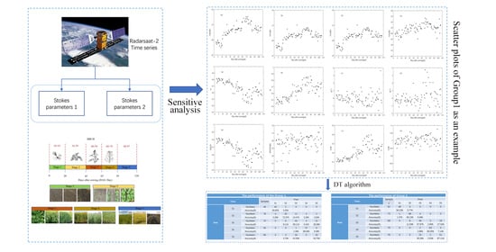
:Accurate and timely knowledge of crop phenology assists in planning and/or triggering appropriate farming activities. The multiple Polarimetric Synthetic Aperture Radar (PolSAR) technique shows great potential in crop phenology retrieval for its characterizations, such as short revisit time, all-weather monitoring and sensitivity to vegetation structure. This study aims to explore the potential of averaged Stokes-related parameters derived from multiple PolSAR data in oilseed rape phenology identification. In this study, the averaged Stokes-related parameters were first computed by two different wave polarimetric states. Then, the two groups of averaged Stokes-related parameters were generated and applied for analyzing averaged Stokes-related parameter sensitivity to oilseed rape phenology changes. At last, decision tree (DT) algorithms trained using 60% of the data were used for oilseed rape phenological stage classification. Four Stokes parameters (, , and ) and eight sub parameters (degree of polarization , entropy , ellipticity angle , orientation angle , degree of linear polarization , degree of circular polarization , linear polarization ratio and circular polarization ratio ) were extracted from a multi-temporal RADARSAT-2 dataset acquired during the whole oilseed rape growth cycle in 2013. Their sensitivities to oilseed rape phenology were analyzed versus five main rape phenology stages. In two groups (two different wave polarimetric states) of this study, , , , , , , and showed high sensitivity to oilseed rape growth stages while , , and showed good performance for phenology classification in previous studies, which were quite noisy during the whole oilseed rape growth circle and showed unobvious sensitivity to the crop’s phenology change. The DT algorithms performed well in oilseed rape phenological stage identification. The results were verified at the parcel level with left 40% of the point dataset. Five phenology intervals of oilseed rape were identified with no more than three parameters by simple but robust decision tree algorithm groups. The identified phenology stages agree well with the ground measurements; the overall identification accuracies were 71.18% and 79.71%, respectively. For each growth stage, the best performance occurred at stage S1 with the accuracy of 95.65% for Group 1 and 94.23% for Group 2, and the worst performance occurred at stage S3 and S5 with the values around 60%. Most of the classification errors may resulted from the indistinguishability of S3 and S5 using Stokes-related parameters.
1. Introduction
Knowledge of crop phenology is significant to precision farming for planning or triggering cultivation practice such as irrigation, fertilization and so on. Timely and accurate knowledge of crop phenology is crucial for government organizations giving precise crop productivity forecasts and making correct agriculture policy decisions [1,2,3]. Remote sensing data, with the capability to monitor crop growth conditions by spatial-temporal image acquiring, have been used for large-scale crop phenology estimation for decades. This definitely requires the frequent acquisition of images over the entire crop growth cycle or at least at key growth stages. Optical sensors have the ability to identify several crop growth stages but are limited in data coverage at some key growth stages due to haze, cloud and rain impeding its effective data acquisition [4,5]. Synthetic aperture radar (SAR) sensors, with the capability of all-weather data acquiring, penetrating deeper into vegetation than optical sensors, are sensitive to the shape, structure and dielectric constant of vegetation scatterers, have the capability to provide a better temporal data coverage and crop structure interpretation than optical sensors. Polarimetric synthetic aperture radar (PolSAR) sensors, given not only their day/night and all-weather monitoring capabilities but also their capabilities to detect target shape/scattering orientation changes, seem sensitive to vegetation structure and show great potentiality in crop phenology retrieval and attract lots of interest [3,4,6].
Many studies have exploited the capabilities of polarimetric parameters in crop phenology estimation [1,2,3,4,5,7,8,9]. The potential of polarimetric SAR data for crop phenology monitoring has been well demonstrated in these studies. For example, a large polarimetric SAR feature sets were generated for crop phenology estimation, including backscattering coefficients and their ratios [1,2,8], coherence between different polarimetric channels [1,2,7,8], phase difference between polarimetric channels [1,2,7,8] and decomposition parameters and developed parameters from different polarimetric decomposition algorithms [3,4,5,9]. Since SAR sensors, especially polarimetric SAR sensors have a relatively low temporal resolution than optical sensors, in several previous studies, crop phenology estimations using SAR data had been approached as a classification problem. Then, the questions such as how many stages can be identified and how should the optimal boundaries of the stages been determined were discussed [8,9]. In addition, dynamic filtering algorithms including Kalman filtering and Particle filtering approaches were developed to estimate crop phenology. These algorithms determined crop phenology along a numerical scale rather than phenology intervals in classification methods. Transition matrix construction is the key of using dynamic filtering algorithms for phenology estimation [5,7]. As the revisit time intervals of the polarimetric SAR sensors decrease, machine learning algorithms such as random forest (RF) [3], K-Nearest Neighbor (KNN) [10], Support Vector Machine (SVM) [8], Complex Wishart Classifier [11] and the Multi-class relevant vector machine (mRVM) [9] are applied in crop phenology estimation.
Although previous studies indicate that crop phenology could be retrieved from polarimetric parameters, most of the extracted polarimetric parameters focus on the target scattering mechanism but ignore the characterizations of the scattering waves, which also show better performance in crop monitoring [12,13,14]. Moreover, parameters extracted according to scattering wave characterizations could not only be used for fully polarimetric data but also for dual-polarimetric data, especially in the period when we can utilize freely accessible dual-pol SAR datasets from the Sentinel-1 mission and more compact polarimetric datasets from RADARSAT Constellation Mission (RCM) and Advanced Land Observing Satellite 2 and Phased Array type L-band Synthetic Aperture Rader 2 (ALOS-2 PALSAR-2). Moreover, these datasets are also effective complement datasets for the low temporal resolution of present quad-polarimetric SAR data acquisition.
Stokes parameters and their developed parameters, which describe the scattering powers directly, are more powerful for dealing with the depolarization information than the decomposition parameters extracted from coherence/covariance () matrix since they can describe the partially polarized scatter based on Born–Wolf wave decomposition theory [15]. Several recent studies on compact polarimetric application utilized these parameters for crop biophysical parameter estimation, and satisfactory results have been achieved for rice, rape oilseed growth monitoring and rice phenology estimation [2,16,17,18]. Since each Stokes vector is related to a polarization state of the incident wave, the averaged Stokes parameters with different assumed incident wave states can provide more information for crop monitoring. Previous studies focused more on compact polarization, which also uses the Stokes-related parameters, but it only has one mode polarization state. Other polarization states, which can also be described using averaged Stokes parameters, were not fully explored, especially for crop phenological stage identification [17,18]. In this study, the concept of averaged Stokes parameters developed based both on compact polarimetric SAR parameter extraction theorem and Poincare sphere were proposed and exploited to estimate rape oilseed phenological stages. We assess the performance of the averaged Stokes-related parameters in oilseed phenological stages over the joint experiment for the crop monitoring test site in Hailar of Inner Mongolia, China. The averaged Stokes-related theory was interpreted and analyzed in this study. Phenological stage estimation was thought as a classification problem in this study and decision tree (DT) methods were selected as the classifiers.
2. Materials and Method
2.1. Study Area and Ground Campaign
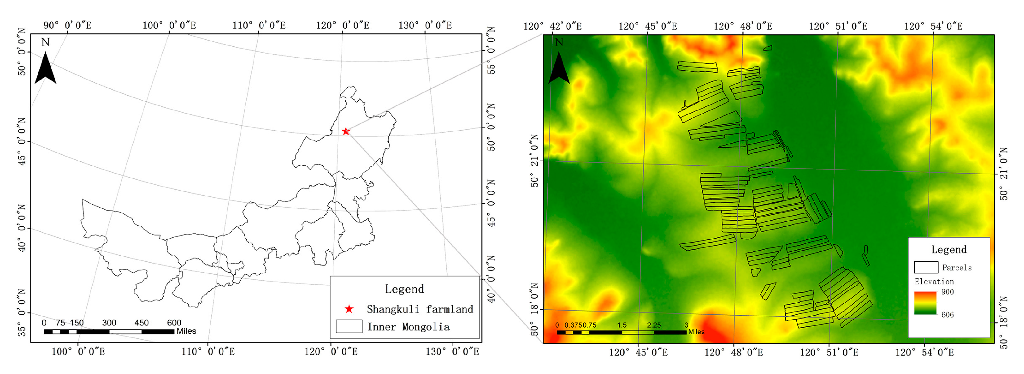
The study was carried out over the parts of Shangkuli farmland located in Hailar of Inner Mongolia, Northeast China (Figure 1). The land is relatively flat with slopes less than 3°. Oilseed rape and wheat constituted the major crops while other minor crops such as soybean was also planted in a few fields. Rape is cultivated once a year during the May to August season. The cultivation period lasts about 115–140 days; among the 85 samples data used in this paper, the earliest sowing date of the oilseed rape was on 8 May 2013, and the latest sowing date was on 31 May 2013. Readers are referred to our previous work [16] for further description of the terrain and climate details of the study area.
A complete description of the ground measurement methodologies was provided in [16]. We measured several crop biophysical parameters including leaf area index (LAI), plant height, surface soil moisture, above-ground biomass (fresh and dry weight per square meter) and plant water content. These parameters were collected synchronous with satellite overpass within a lag of no more than one day of the date that each RADARSAT-2 data acquired. In each campaign, 11–14 representative oilseed rape fields were surveyed. For each field, the sowing date was recorded and its phenology was described according to the BBCH-scale developed by Weber and Bleholder [19]. The field states were recorded by GPS tagged photos.
2.2. SAR Data Set
During the oilseed rape cultivation period in 2013, five full polarization RADARSAT-2 data were acquired from 23 May to 27 August, imaging the entire oilseed rape phenological cycle. Five RADARSAT-2 SLC (Single Look Complex) images taken on May 23, June 16, July 10, August 3 and August 27, respectively, were used in this study. All of the images were collected with the same mode, beam, incident angle and orbit pass to reduce the influence of sensor parameters. Precipitation and temperature were recorded by the in- situ weather station to provide meteorological conditions for image collections as well as for field campaigns. The detailed information of image acquisition parameters, precipitation and temperature information can be found in [16,17].
2.3. Definition of Phenological Stages
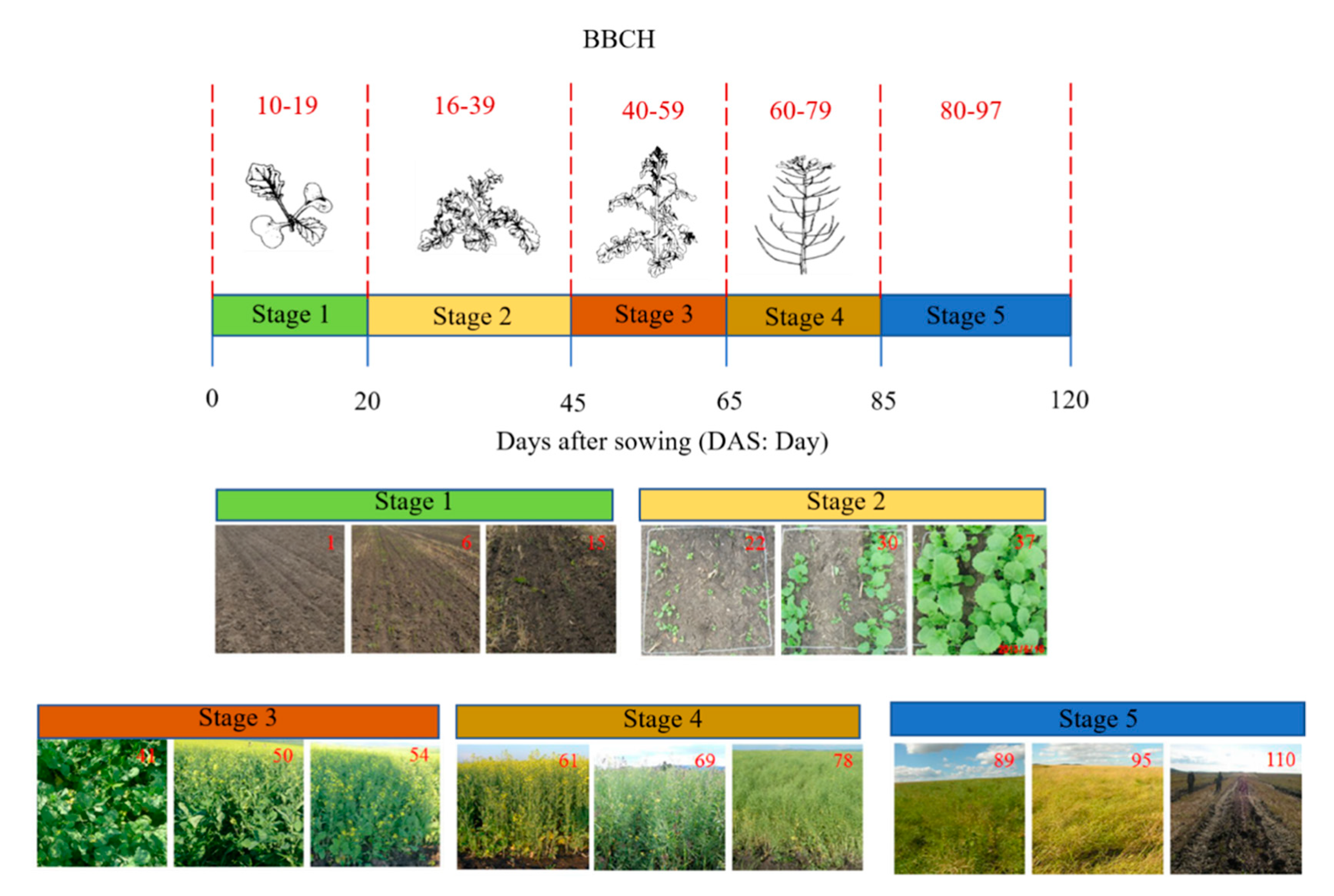
In this study, oilseed rape phenology estimation is thought of as a classification problem. Each phenological stage is considered as an individual class. Each class of oilseed rape phenology is defined on the base of the crop appearance inside its life cycle and also the SAR data available to date. The appearance of oilseed rape results from its morphological and physiological development. By considering the appearance within one stage does not change much but differs strongly between two different stages, the phenology of oilseed rape in this study is divided into 5 stages. The BBCH-scale developed by Weber and Bleiholder (1990) is used to code the plant’s appearance at each phenological stage. However, BBCH code, which is defined by a small set of integer values specific for each crop group, is unsuitable for use as the state variable in crop growth stage estimation [5]. Thanks to the relationship between day after sowing (DAS), growing degree days (GDD) and crop phenological stages [5,9], DAS is selected as the proxy variable of oilseed rape phenology to describe the temporal profile of polarimetric SAR information during the oilseed rape entire growing season. The phenological stages, their corresponding BBCH-codes, DAS and plant images taken from Weber and Bleiholder (1990) and taken at each field campaign time are illustrated in Figure 2.
2.4. Analysis of Phenological Stages
In this study, five main phenological stages were defined for the entire growth cycle of oilseed rape. At each stage of them, oilseed rape has particular features and aspects of the plant development as the change of DAS. At the phase of Stage 1, when the first RADARSAT-2 image was acquired, most oilseed rape fields had just been sown or were at the beginning of crop emergence. This stage is characterized by development from dry seed to hypocotyl with cotyledons growing towards soil surface. The next main stage (Stage 2) starts from plant emergence and ends with fully developed plants. At first, cotyledons are completely unfolded; then the first leaf is clearly visible and additional leaves are unfolded up. Following side shoots begin to develop and 9 or more side shoots are developed and detectable at the end of this stage. The phase of Stage 3 comprises a wide range of plant conditions including stem elongation with extended internodes, flower buds presented from being enclosed by leaves to first petals being visible, first flowers opening to the end of flowering. At stage 4, oilseed rape begins to pod and it is characterized by increasing pod size and number. Finally, Stage 5, including ripening and senescence, also constitutes a period with many changes in the plants. Oilseeds appear green and pod cavities become filling. Then, 10% oilseeds appear dark and hard, pods become ripe until nearly all pods ripe, seeds dark and hard. At the end of this stage, on the moment of harvest, water content of the plants changes up and down, the plants become dead and dry, their structure is mostly random and number of leaves decrease.
2.5. Extraction of Averaged Stokes-Related Parameters
2.5.1. Rationale
The objective of selecting Stokes-related parameters is to generate a group of unbiased polarimetric characterizations of the observed scene. Radar generates the transmitted wave and backscattered wave is a quasi-monochromatic partially polarized electromagnetic wave which is backscattered from the radar irradiation scene. This kind electromagnetic wave could be represented by four members from the Stokes vector containing all of the available polarimetric and un-polarimetric information. We also call these four members Stokes parameters [20,21,22]. The names of the Stokes parameters vary depending on the specific discipline preferred by their user. In this study, their forms are shown as in equation (1), where means the member of Jones vectors. For the detail information about the equation, readers are referred to the literature [15,22].
The four members were determined from information conveyed in the observed filed. Each of the Stokes parameters is an averaged quantity. The first Stokes parameter is directly proportional to the power density being carried by the backscattered wave. It includes the polarized and depolarized backscattered signals. The other three parameters represent the polarized portion of the backscattered wave. The second parameter indicates the tendency of the polarization to be more horizontal or vertical, while the third and fourth indicate the ellipticity of the wave’s polarization. The four Stokes parameters for a pixel show a polarization state of the backscattered wave and they could be located on/in a unit sphere named Poincare sphere geometrically. Since the Stokes parameters are based on a wave polarimetry framework, they allow for analyzing the average polarization state of the backscattered wave. It has the following characters: (1) Stokes parameters could be used for extracting depolarization information of a partially polarized wave; (2) Stokes parameters could be extracted directly from the 2 × 2 Jones matrix without any assumptions; (3) The decomposition expressed by three physical components of the averaged Stokes parameters, i.e., the total scattered intensity , the degree of polarization and the completely polarized wave components () obey the general physical laws and avoid the conflict among the physical meaning, uniqueness and completeness. Meanwhile, the completely polarized wave components can also be described by several parameters coming from the Poincare sphere, which make the parameters visible to the readers.
The key theory for averaged Stokes-related parameters proposed in this study is the “polarization synthesis” based on the four Stokes parameters (Woodhouse, 2006). As we know, if a target has a preferred shape or orientation, then differently polarized incident waves will result in backscattered echoes, whose polarization state is, in principle, related to the target’s shape or orientation. Using four Stokes parameters and polarization synthesis technique, we can simulate the response for any arbitrary combination of transmit and receive polarization. Then we can collect the target response at each polarimetric states. The polarimetric synthesis procedure is often achieved by multiplication of by the Stokes vectors for the transmitted and receive polarizations. is the Kennaugh matrix, in which the scattered wave is described in the receiving antenna reference frame so that both the incident wave and the scattered wave are described from the point of view of the antenna. Here, it is given by (2) [23]:
In Equation (2), is a 3 3 Hermitian matrix; it is also called coherence matrix. The backscatter power of the target for a given combination of transmitted and received ellipticity and orientation angles is given by
where and are ellipticity angle and orientation angle for the polarimetric ellipse, respectively, the subscript and describe the received and transmitted polarization, respectively. Since the range of and are polar coordinates within a Poincare sphere, the synthesized polarization response , for any given and , can be considered as an intensity pattern of the target across the sphere.
2.5.2. Stokes-Related Parameter Calculation from the Four-Member Stokes Parameters
According Equation (3), the different values of four Stokes parameters and their sub parameters such as , and mentioned above describe different polarization states of the backscattering wave of the observed target. The averaged Stokes-related parameters of several polarization states give more information of the observed target than only one polarization state. Among the synthesized polarization, three special polarization states were often used. The three polarization states are transmitting with a H linearly polarized field and receiving the resulting H and V backscatter components coherently, transmitting with right a circular polarized field and receiving the resulting H and V backscatters components coherently, and transmitting with a linearly polarized field at 45° and receiving the resulting H and V backscatters components coherently. The last two polarization states are commonly used as and compact polarization [15,22]. is the most effective compact polarization proposed in recent two decades, and many research studies confirmed its effectiveness in crop phenology identification [2,18]. Classification accuracy acquired by compact polarization data was proven to be very nearly as good as fully polarized data and the difference between them is negligible [22]. However, the linear polarization with H or V transmitting but receiving with H and V, the dual polarization of which is usually used in classical dual-pol modes, has not been fully explored with a Stokes-related theorem so far.
In this paper, two sets of averaged Stokes-related parameters based on linear polarization were calculated to analyze their potentiality in crop phenology identification. One set of averaged Stokes-related parameters was calculated from the linear polarization with H transmitting but H and V receiving (Group1), and the other was from the linear polarization with V transmitting but H and V receiving (Group2). The performance of the two group-averaged Stokes-related parameters on oilseed rape phenology estimation was presented here. In this paper, the averaged Stokes-related parameters including the four basic Stokes members , the degree of polarization (), entropy (), ellipticity angle (), orientation angle (), degree of linear polarization (), degree of circular polarization (), linear polarization ratio () and circular polarization ratio () were calculated as parameter sets of Group 1 and Group 2, respectively. The physical interpretation of each Stokes-related parameter and their equations are shown in Table 1 [24,25].
2.6. Decision Tree (Dt) Algorithm Training and Validation
Previous studies, which evaluated the classification performance of the different classifiers, have reported that the DT classifier provides high accuracy and efficiency classification results, especially for the case of nonlinear relationships between features and classes [1,2]. In this study, a univariate DT with the Gini index attribute is used for distinguishing the different phenological stages of oilseed rape. The performance of the DT algorithm relies on the representativeness of the training datasets. In this study, Stokes-related parameters were computed from each pixel of the parcels and then averaged at parcel level according to the value of day after sowing. In total, 85 data points were used for DT training and validation. Of this total, we randomly selected 60% of them as training data, while the left 40% of the datasets were considered for validation. Since the 60% training data are randomly selected, the DT functions are more flexible and can produce different classification results, the classification procedure for oilseed rape phenological stages estimation were repeated 10 times and the averaged result was selected as the classification results and terminal accuracy.
2.7. Oilseed Rape Phenological Stages Estimation Scheme
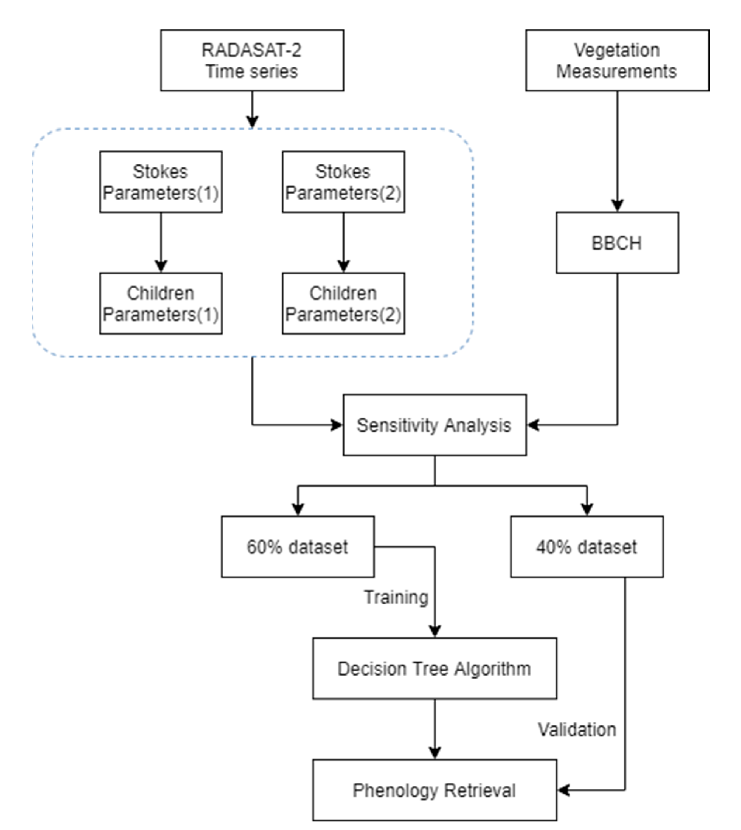
The current study aims to explore the potential of averaged Stokes-related parameters in oilseed rape phenological stage identification. Figure 3 shows the flowchart of the oilseed rape phenology estimation procedure with averaged Stokes-related parameters. At the first step, three groups of Stokes parameters were calculated according to [24] and then the one with averaged values were chose for analyzing their response to oilseed rape during its entire growth season. In the flowchart, Stokes parameters (1) and Sub parameters (1) are the calculated as 12 Stokes-related parameters from Group1, Stokes parameters (2) and Sub parameters (2) are calculated as 12 Stokes-related parameters from Group2 in Section 2.5.2. Then, the sensitivity analysis was centered on the evolution of the Stokes-related parameters for the monitored parcels over the entire growth cycle. For each parcel, we calculated one averaged observation by averaging performance in the whole area of the parcel. Next, all of the analyzed Stokes-related parameters had been computed for all of the images and have been averaged by DAS. Finally, the Stokes-related parameters had been plotted as a function of DAS. At last, the phenology estimation by exploiting the temporal behavior of 12 averaged Stokes parameters were classified by decision tree algorithms.
In this procedure, Full polarimetric data measured objects in each resolution element with complex scattering matrix ; it was extracted from the original RADARSAT-2 SLC images using PolSARpro4.2 toolbox, followed by boxcar filter to moderate speckle effects. The incident waves were supposed and used to calculate Stokes parameters by a unit Jones vector through Equation (1), respectively.
3. Results and Discussion
3.1. Stokes and Child Parameter Response to Rape Phenology
Twelve key Stokes and their sub parameters are analyzed and presented in the following. They are divided into three main categories as follows according to their physical interpretations.
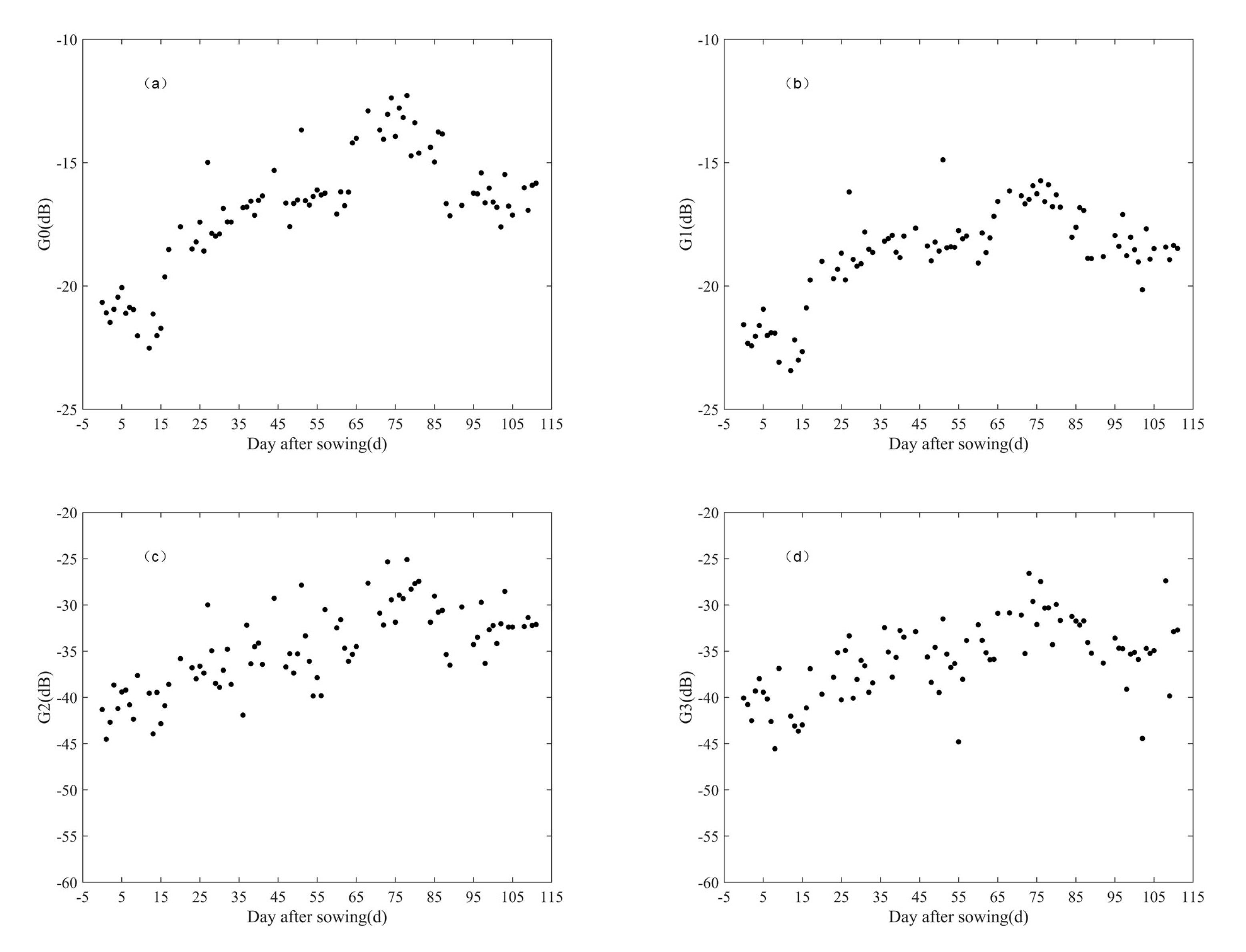
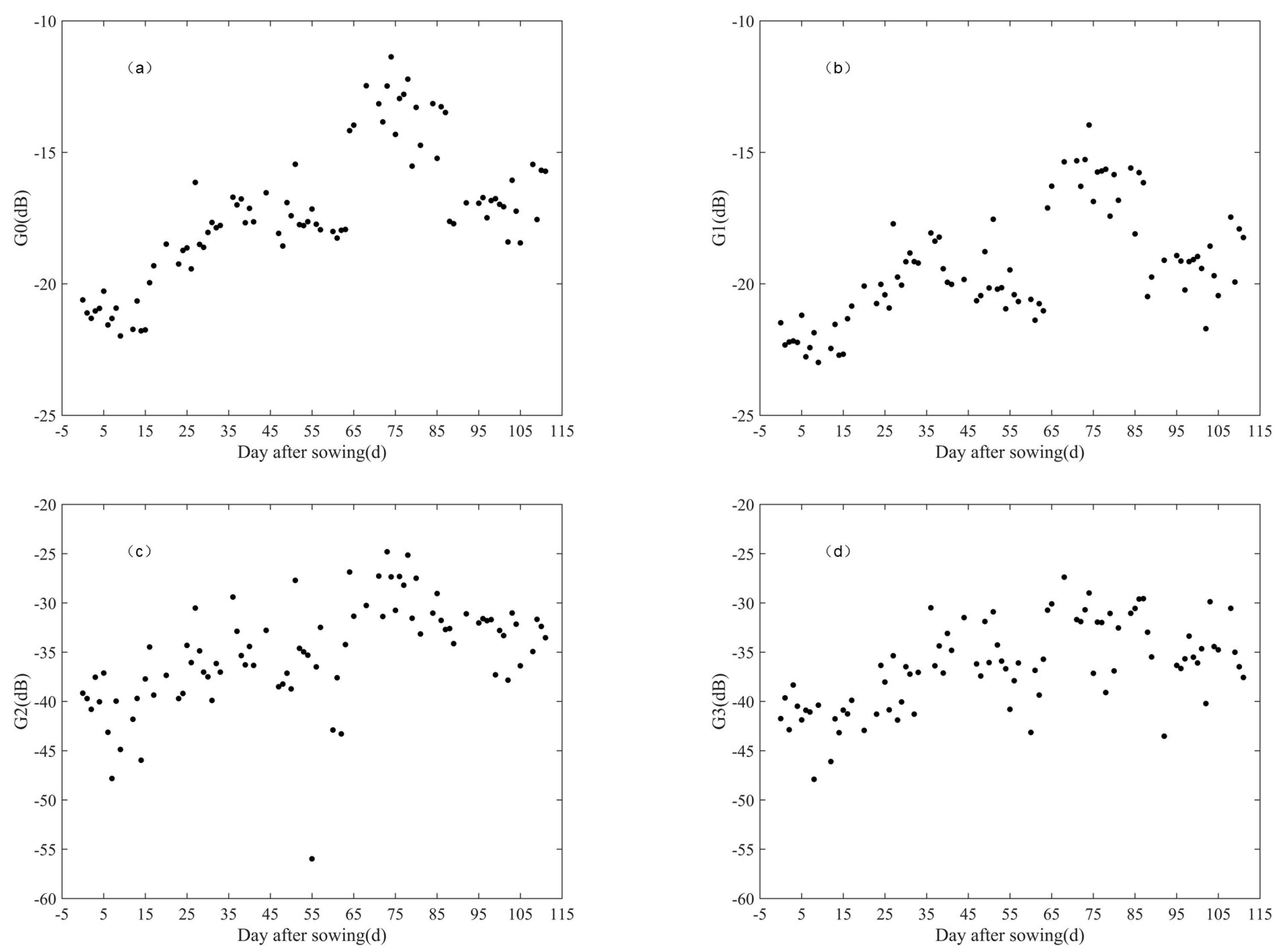
The original Stokes parameters, including , , and were divided as the first category. The response of the original averaged Stokes parameters to the advancement of oilseed development was measured by DAS at parcel level. The response of each parameter was described by each subplot of Figure 4 and Figure 5. A total of 85 samples are graphed in each scatter plot in Figure 4 and Figure 5, the trends of original Stokes parameters of Group 1 shown in Figure 4 were similar with the trends of Group 2 shown in Figure 5. The trends of , , and in Figure 4 and Figure 5 during the whole oilseed growth cycle were coincident with the evolution of three growth parameters, biomass, crop height and Leaf area index (LAI), which we gave in our previous work [16]. Among the three crop growth parameters, the biomass evolution trend shows a best fit for these original Stokes parameters. At stage 1, all values of the four Stokes parameters showed lowest and kept steady during the entire stage 1, then they began a gently increasing slope at stage 2. They showed a gently decreasing trend at stage 3 and form a peak with a sharp slope at stage 4 and rising to a maximum at approximately DAS = 75. The curve of the scatter plots ended in an obvious decrease at stage 5. Although all of the four parameters had a similar trend during the whole oilseed rape growth cycle, showed best performance for oilseed rape phenological period response. Among them, had the highest values during the whole growth cycle, its dynamic range were from −22 dB to −12 dB for Group1 and from −21 dB to −11 dB for Group2. At stage 1, had the lowest value of in two groups, the lower scattering value in this stage may result from the dominated soil scattering since the plant was just sown or emerging through the soil surface with plant heights not exceeding 5 cm. At stage 2, the values of were gently increased to −19 dB since the increasing of plant scattering increases with the growth of oilseed rape leaves. Group 1 and Group 2 kept increasing around 16 dB at the earlier stage of stage 3 with more leaves adding and growing up. At the later stage of stage 3, the values were shown to be gently decreasing, which may result from the falling of large leaves at the oilseed rape canopy and more soil under the canopy showing up. With the main stem emerging at approximately DAS = 61, increased to −16 dB then decreased to −10 dB at stage 4 since the dihedral response from the main stem and ground surface. At stage 5, the ripening and senescing of plants resulted in the falling of leaves and decreasing of water content that led to the decreasing of values around −17 dB in two groups. showed a smaller dynamic range from −23 dB to −14 dB during the whole oilseed rape growth cycle compared with , while the trend of was similar with . Its tendency was quite different with our previous study where the distinction between and was obvious. In the HCP compact mode, the values of , and showed even poorer performance varying with the evolution of plant growth. However, during the whole process of rape growth, the values of the Group 1 of Stokes parameters were more aggregated than those in the Group 2.
The performances of and agreed well with our previous work [16] on compact polarization data applying in crop growth parameters estimation; however, the results of and were quite different. It was probably explained by the fact that our previous research assumed right circular polarization as the transmitting channel, which may lead to different backscattering from objects. The potentiality of averaged for land-cover classification was also stated by Shang et al. (2015) in [15]; however, the capabilities of , and were left unexplored in their study.
3.1.1. Sub Parameters from Poincare-Sphere or Decomposition Methods
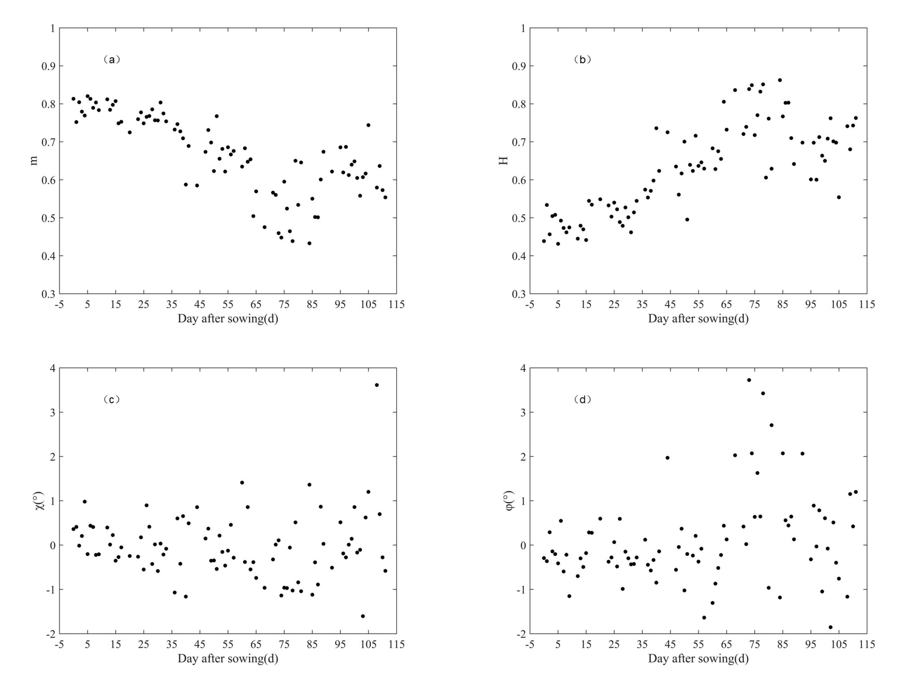
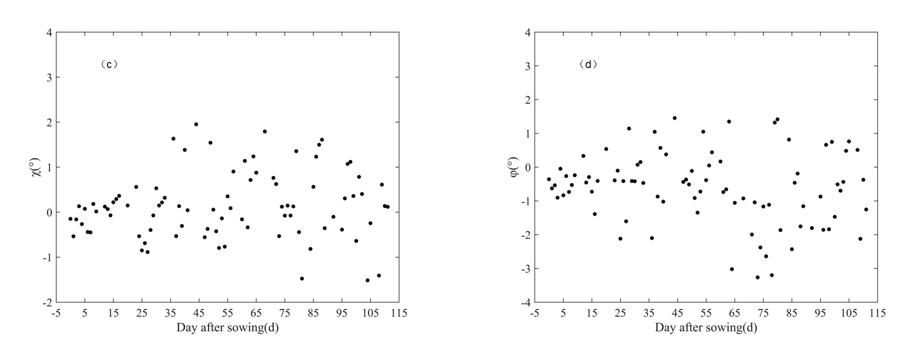
Previous studies on compact polarization applications proved that Stokes sub parameters were useful for crop mapping and monitoring. Figure 6 and Figure 7 presented the evolution of the four more useful sub parameters in both of Group 1 and Group 2 as a function of DAS. The four Stokes-related parameters were the degree of polarization (), entropy (), ellipticity angle () and orientation angle (). Among them, and were two different ways to describe the degree of randomness of target scattering, and derived from Poincare-sphere were robust choices for describing the shape and orientation of polarized ellipticity. The shape and orientation of polarized ellipticity characterized the scattering information of objects in the scattering scene.
In accordance with Figure 4 and Figure 5, the trends of , , and in Group 1 and Group 2 were also similar. Figure 6a and Figure 7a resampled with four different ranges during the whole oilseed rape growth cycle: 0.7–0.8 during stage 1 and stage 2 while the values from Group 1 were slightly higher than those from Group 2; the values for stage 3 in the group 1 were 0.5–0.7; while the values for stage 3 in the group 2 were 0.4–0.6, and in the group 1, 0.4–0.6 was in stage 4, while in the group 2, 0.5–0.6 was in stage 4 and the value of stage 5 in both the first and second groups was around 0.6. Note that low degrees of polarization were equivalent with high entropies and vice versa. Entropy in Figure 6b and Figure 7b was less than 0.5 during stage 1 and 2 before stem elongation, and increased to 0.7 at stage 3 with stem elongating but large leaves withering and falling. reached its peak when it increases around 0.9 and then kept a flat line during the whole stage and stage 5. The higher values of lower m values in stage 4 and stage 5 may result from the crop leaves accumulating, bolts and flowers developing, canopy expanding that lead to greater scattering randomness. tapered to 0.8 at stage 5 with ranging from 0.5 to 0.6 meant withering leaves and pods decreased some scattering randomness. The combination of the two parameters showed their capability of distinguishing the early phenological stage. The findings in our study agreed with [2,17], even though the crops were different in these studies. However, compared our previous work on compact polarimetric parameters, the range of values in this study were quietly different. In this study, the values of Group 1 ranged from 0.82 to 0.43 and in the Group 2 it ranged from 0.85 to 0.45, while in previous works they ranged from 0.7 to 0.25 [16]. values in the study of Lopez–Sanchez on rice ranged from 0.9 to 0.2 [2]. The phenomenon demonstrated that the average procedure of Stokes-related parameters reduced the sensitivity of m values to the crop growth stage changes.
and were addressed as robust parameters for classification in previous studies, especially , which was used for distinguish odd and even scattering mechanism with its negative and positive sign. However, they had poor performance in this study. The trends of and in Group 1 and Group 2 shown in Figure 6 and Figure 7c,d respectively presented the contribution of and in different phenological stages. Both of them showed small dynamic range during the whole crop growth cycle. For , the value of Group 1 was approximately −0.03° and the value of Group 2 was around 0.12°. For , the value of group 1 was approximately 0.06° and the value of group 2 was around 0.06°. The reason for the small dynamic probably because the assumed transmit was linear polarization or the averaged values without signs decreased their sensitivity to target scattering. In converse with this finding in our study, previous studies showed better evolution performance of versus crop phenology. Note that, parameter, used in previous studies, was assumed the transmit polarization of circular [2,16,17].
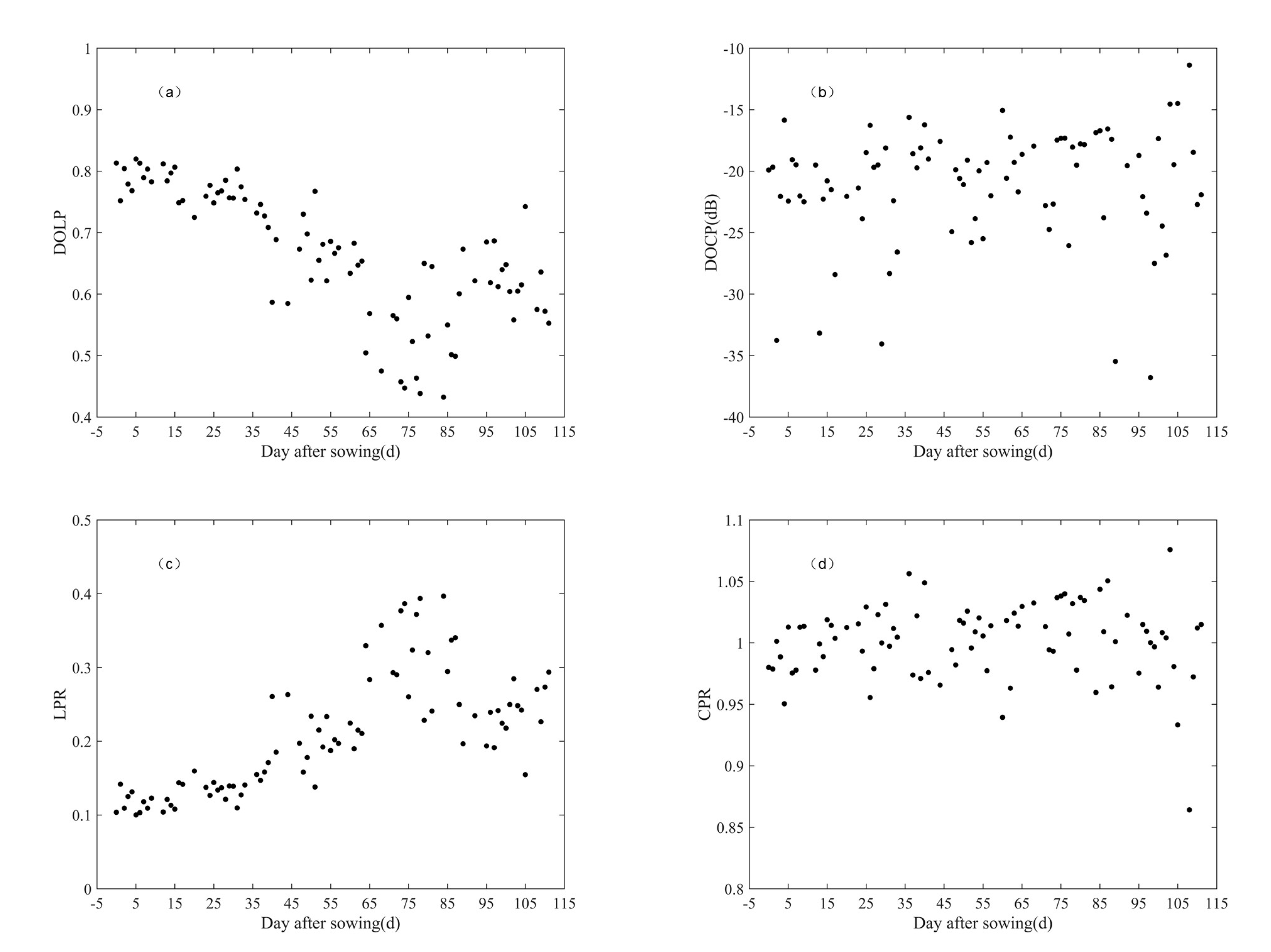
3.1.2. Sub Parameters Related to Linear of Circularity Ratio and Degree
, , and were first published by George Gabriel Stokes for optical field observation and quantitative measuring. They were first applied in SAR information extraction in 2006 by Raney for dual-polarized SAR data [24]. Then, several of them were used for compact SAR data applications. In this study, Figure 8 and Figure 9 showed the evolution of the four averaged parameters versus DAS. and , which had better performance in compact SAR data for crop classification and phenology retrieval in previous studies, were quite noisy in more parts of the phenological cycle and seemed difficult to distinguish oilseed rape growth stages. Conversely, and showed obvious sensitivity to the evolution of oilseed rape growth stages when their range scales were stretched with logarithmic function. decreased as the oilseed rape grows because of the increased non-linear polarization components from volume scattering of developed oilseed rape. Then, it gently increased at stage 4 with the contribution of even scattering mechanism caused by elongated stem and falling crop leaves. kept increasing during almost all of the crop growth cycle. The dynamic range varied with the change of each growth stage. The finding agreed with [6] in which HH/VV were sensitive to the rice structure and may be helpful in monitoring crop growth.
3.2. Oilseed Rape Phenology Classification Using DT Method
After analyzing the sensitivity of averaged Stokes-related parameters to changes in oilseed rape phenology, in this section we represented the classified oilseed rape phenology stages using DT algorithms. Since the algorithms were trained by randomly selecting 60% of the dataset, the constructed DTs were different at each training operation procedure. We repeated DT algorithm 10 times to reduce the classification randomness and also improve the objectiveness of the classification results. In each repetition process, 52 samples were randomly selected from 85 samples for training, and the remaining 34 samples were verified for classification results, Table 2 showed the phenological classification results of Group 1, Table 3 showed the results of Group 2. Since the available ground data were expressed at parcel level, the procedures of classification and validation were carried out at parcel level too. The comparisons of the ground data against the estimated results were performed by computing the number and percentage of parcels assigned to each phenological stage correctly and wrongly. In each table, to ease the reading of the tables, the correct classified numbers were colored with yellow color while the wrong ones were colored with orange color.
Note the result of repeating DT 10 times given in Table 2 and Table 3; the DT algorithm combined with Stokes-related features showed different classification performance at different crop phenological stages. In the Group 1, S1 had the highest value of the frequency of average overall classification accuracy equaling 95.65%, the second one was stage 4 (S4, 89.06%), then S2 (72.37%), S3 (58.11%) and the last one was stage 5 (S5, 53.75%). In the Group 2, similar as the Group 1, S1 had the highest value of the frequency of average overall classification accuracy equaling to 94.23%, but the second one was stage 2(S2, 93.15%), then S4(90.00%), S5 (67.11%) and the last one was stage 3 (S5, 57.97%). Among the five phenological stages, S1 had the highest correct rate, but the classification errors showed that S1 was always wrongly classified as S2. For the later growth stage of S1 and the early growth stage of S2, the vegetation was small and SAR backscattering was thus mainly influenced by soil roughness and moisture which resulted in the difficulty to distinguish these two stages [17,26]. For the case of S4, the correct rate of S4 of the two groups was around 90%, and it revealed the capacity of Stokes-related parameters in identifying the oilseed rape growth state at stage 4. At S4, the oilseed rape began to pod, a large volume of pods created significant multiple scattering and resulted in the obvious difference of the value of , , , , , and . When these features were input in DT algorithms for both training or validation, single feature of them was sufficient to identify the stage [3]. Next S4 and S1 was S2, in the Group 2, the correct classification was 93.15%, 5.48% were misclassified as S3 and 1.37% as S1; in the Group 1, the correct classification was 72.37%, and S2 was wrongly classified to S1, S3, S4 and S5. The misclassification rate of S3 was high; for example, both in Group 1 and Group 2, only about 58% results of the classification were correct, while about 30% of the classification results were wrong. For S5, S5 was always wrongly classified into S3, 50% of the S5 in Group 1 were misclassified as S3, and 60% of the S5 in Group 2 were misclassified as S3. At the early stage of S3, large leaves in the bottom canopy layer kept growth or began to wither and fall, while at the middle or later stage of S3, stem elongation began to occurred or got more visibly extended internodes. The growth of crop state at S3 resulted in mixed scattering mechanisms at this stage. Meanwhile, at S5, the mixture of scattering mechanisms was still obvious, although the mixture of scattering mechanisms was different from S3, but the features extracted from Stokes were inefficient to distinguish them. Even at S5, the crop began to ripen with decline of plant water content and then resulted in a decrease of scattering power as shown the variation of , it was difficult to distinguish by the features that characterizing the power variation. Several literatures reported the ratio of several polarimetric features had an ability to distinguish the variation of scattering power; however, the combination of Stokes-related features need to further explored to distinguish the difference between S3 and S5 [9,17,25].
In general, the overall classification accuracy of the Group 1 was 71.18%, and the value for Group 2 was 79.71%. Previous research demonstrated good performances on phenological estimation with different stage boundaries (different phenological labelling cases), which included three major stages, five stages, and seven stages. The highest accuracy of these studies for the overall phenological stages estimation was 96%, while the lowest was around 67.0%. For the accuracy of each stage, the highest value was 100%, while the lowest value was 48.4% [8,9,10]. The study combined SAR polarimetric features and DT algorithm performed on rice showed highest accuracy of 91.4% and lowest one of 48.8% [8]. Yang et al. compared the difference of estimation results with different rice phenological labelling cases, including 6 stages, 8 stages and 10 stages. Their results demonstrated the influence of phenological labelling on the estimation accuracy of crop phenological stages. They also concluded that 8 stages were best phenological labelling way to get the best phenological estimation results, the highest accuracy was got at stage 1 with the value of 93.5%, while the lowest value was got at stage 6 with the value of 83.2% [9]. Denoting the phenological estimation results obtained by combining Stokes-related features and DT algorithms in this study, and the comparison with previous related studies, then it could be seen that the Stokes-related SAR features had great potentiality to estimate crop phenological stage.
4. Conclusions
The study aimed to explore the potentiality of averaged Stokes-related parameters for the estimation of oilseed rape phenological stages at a parcel level by using decision tree algorithms. In this study, four Stokes parameters and several sub parameters calculated from four original Stokes parameters were computed with the assumption of receiving orthogonal horizontal and vertical waves but transmitting horizontal and vertical waves, respectively. Then the averaged Stokes parameters and their sub parameters derived from the two groups of Stokes parameters were applied for analyzing sensitivity to oilseed rape phenology. Then, five phenology intervals of oilseed rape were identified with three parameters by simple but robust decision tree algorithms. Most Stokes-related parameters showed high sensitivity to the development of the oilseed rape structure. Given the dramatic changes in the structure of oilseed rape during the whole growth cycle as it moves from the accumulation of leaves, elongation of stems, formation of flower buds, filling and ripening of buds, senescence of plants, Stokes-related parameters including , , , , , , and showed obvious evolution versus the oilseed rape growth. A comprehensive analysis of the relationship between these parameters and rape growth stages revealed the potential of averaged Stokes-related parameters for oilseed rape phenological stage identification. However, other Stokes-parameters, including , , and , which showed good performance for classification in previous studies, were quite noisy during the whole oilseed rape growth circle and showed unobvious sensitivity to the crop’s phenology change. The reason may because of the assumed incident wave’s horizontal and vertical polarization, which have few other polarized powers in the received channel. However, it needs to be studied further in the future. With the inputs of Stokes-related parameters, the DT algorithm provided robust phenology retrieval results; the overall average estimation accuracy of five oilseed rape phenological stages in two Groups is 71.18% and 79.71%, respectively. Meanwhile, the best estimation accuracy for each stage was 95.65%. The results revealed the potentiality of Stokes-related parameters in crop phenological stage estimation, especially for the oilseed rapes growing at S1, S2 and S4 stages. The novelty of this study stems from the fact that it is a first step towards the retrieval of crop phenology using averaged Stokes parameters and their sub parameters. The analytical findings have the potential to serve as a reference for further studies that would attempt to relate the crop phenological stages to averaged Stokes parameters, which can describe depolarization information better than polarimetric decomposition parameters. An obvious limitation of this study was its application in real dual polarization data. In future studies, more dual polarization data should be explored, moreover, the performance and estimation accuracy of crop phenological stages are affected by phenological labelling ways and classification algorithms. In the future, the performance of Stokes-related parameters should be explored with different phenological labelling ways and different classification algorithms.
Author Contributions
W.Z. is the principal author of this manuscript and she had written the majority of the manuscript and also contributed during one phase of the investigation. Y.Z. and Y.Y. contributed to the experiment performance, the selection and interpretation of the methods and some portions of the written manuscript. E.C. supervised the method and the written of this manuscript. All authors contributed to interpreting results and improving the quality of the paper. All authors have read and agreed to the published version of the manuscript.
Funding
The research was funded by National Natural Science Foundation of China, grant number 31860240 and Science Foundation of Yunnan Education Department, grant number of 2019J0182 and 2020Y0393.
Institutional Review Board Statement
Not Applicable.
Informed Consent Statement
Not Applicable.
Acknowledgments
We thank the National Natural Science Foundation of China (31860240) and the Science Foundation of Yunnan Education Department (2019J0182, 2020Y0393). The authors would like to thank Lu Dendsheng for improving this paper’s language and structure. The authors would like to thank all the crews of field campaign for collecting this successful dataset and the anonymous reviewers for improving the paper.
Conflicts of Interest
The authors declare no conflict of interest.
References
- Lopez-Sanchez, J.M.; Cloude, S.R.; Ballester-Berman, J.D. Rice Phenology Monitoring by Means of SAR Polarimetry at X-Band. IEEE Trans. Geosci. Remote Sens. 2012, 50, 2695–2709. [Google Scholar] [CrossRef]
- Lopez-Sanchez, J.M.; Vicente-Guijalba, F.; Ballester-Berman, J.D.; Cloude, S.R. Polarimetric Response of Rice Fields at C-Band: Analysis and Phenology Retrieval. IEEE Trans. Geosci. Remote Sens. 2014, 52, 2977–2993. [Google Scholar] [CrossRef] [Green Version]
- Wang, H.; Magagi, R.; Goïta, K.; Trudel, M.; McNairn, H.; Powers, J. Crop Phenology Retrieval via Polarimetric SAR Decomposition and Random Forest Algorithm. Remote Sens. Environ. 2019, 231, 111234. [Google Scholar] [CrossRef]
- Canisius, F.; Shang, J.; Liu, J.; Huang, X.; Ma, B.; Jiao, X.; Geng, X.; Kovacs, J.M.; Walters, D. Tracking Crop Phenological Development Using Multi-Temporal Polarimetric Radarsat-2 Data. Remote Sens. Environ. 2018, 210, 508–518. [Google Scholar] [CrossRef]
- McNairn, H.; Jiao, X.; Pacheco, A.; Sinha, A.; Tan, W.; Li, Y. Estimating Canola Phenology Using Synthetic Aperture Radar. Remote Sens. Environ. 2018, 219, 196–205. [Google Scholar] [CrossRef]
- Wiseman, G.; McNairn, H.; Homayouni, S.; Shang, J. RADARSAT-2 Polarimetric SAR Response to Crop Biomass for Agricultural Production Monitoring. IEEE J. Sel. Top. Appl. Earth Obs. Remote Sens. 2014, 7, 4461–4471. [Google Scholar] [CrossRef]
- Vicente-Guijalba, F.; Martinez-Marin, T.; Lopez-Sanchez, J.M. Crop Phenology Estimation Using a Multitemporal Model and a Kalman Filtering Strategy. IEEE Geosci. Remote Sens. Lett. 2014, 11, 1081–1085. [Google Scholar] [CrossRef] [Green Version]
- Kucuk, C.; Taskin, G.; Erten, E. Paddy-Rice Phenology Classification Based on Machine-Learning Methods Using Multitemporal Co-Polar X-Band SAR Images. IEEE J. Sel. Top. Appl. Earth Obs. Remote Sens. 2016, 9, 2509–2519. [Google Scholar] [CrossRef]
- Yang, Z.; Shao, Y.; Li, K.; Liu, Q.; Liu, L.; Brisco, B. An Improved Scheme for Rice Phenology Estimation Based on Time-Series Multispectral HJ-1A/B and Polarimetric RADARSAT-2 Data. Remote Sens. Environ. 2017, 195, 184–201. [Google Scholar] [CrossRef]
- Yuzugullu, O.; Erten, E.; Hajnsek, I. Rice Growth Monitoring by Means of X-Band Co-Polar SAR: Feature Clustering and BBCH Scale. IEEE Geosci. Remote Sens. Lett. 2015, 12, 1218–1222. [Google Scholar] [CrossRef]
- Mascolo, L.; Lopez-Sanchez, J.M.; Vicente-Guijalba, F.; Nunziata, F.; Migliaccio, M.; Mazzarella, G. A Complete Procedure for Crop Phenology Estimation With PolSAR Data Based on the Complex Wishart Classifier. IEEE Trans. Geosci. Remote Sens. 2016, 54, 6505–6515. [Google Scholar] [CrossRef] [Green Version]
- Singha, M.; Dong, J.; Zhang, G.; Xiao, X. High Resolution Paddy Rice Maps in Cloud-Prone Bangladesh and Northeast India Using Sentinel-1 Data. Sci. Data 2019, 6, 26. [Google Scholar] [CrossRef]
- Fikriyah, V.N.; Darvishzadeh, R.; Laborte, A.; Khan, N.I.; Nelson, A. Discriminating Transplanted and Direct Seeded Rice Using Sentinel-1 Intensity Data. Int. J. Appl. Earth Obs. Geoinf. 2019, 76, 143–153. [Google Scholar] [CrossRef] [Green Version]
- Mandal, D.; Kumar, V.; Ratha, D.; Dey, S.; Bhattacharya, A.; Lopez-Sanchez, J.M.; McNairn, H.; Rao, Y.S. Dual Polarimetric Radar Vegetation Index for Crop Growth Monitoring Using Sentinel-1 SAR Data. Remote Sens. Environ. 2020, 247, 111954. [Google Scholar] [CrossRef]
- Shang, F.; Hirose, A. Averaged Stokes Vector Based Polarimetric SAR Data Interpretation. IEEE Trans. Geosci. Remote Sens. 2015, 53, 4536–4547. [Google Scholar] [CrossRef]
- Zhang, W.; Li, Z.; Chen, E.; Zhang, Y.; Yang, H.; Zhao, L.; Ji, Y. Compact Polarimetric Response of Rape (Brassica Napus L.) at C-Band: Analysis and Growth Parameters Inversion. Remote Sens. 2017, 9, 591. [Google Scholar] [CrossRef] [Green Version]
- Yang, H.; Li, Z.; Chen, E.; Zhao, C.; Yang, G.; Casa, R.; Pignatti, S.; Feng, Q. Temporal Polarimetric Behavior of Oilseed Rape (Brassica Napus L.) at C-Band for Early Season Sowing Date Monitoring. Remote Sens. 2014, 6, 10375–10394. [Google Scholar] [CrossRef] [Green Version]
- Zhi, Y.; Li, K.; Long, L.; Shao, Y.; Brisco, B.; Li, W. Rice growth monitoring using simulated compact polarimetric C band SAR. Radio Sci. 2015, 49, 1300–1315. [Google Scholar]
- Weber, E.; Bleiholder, H. Erläuterungen Zu Den BBCH-Dezimal-Codes Für Die Entwicklungsstadien von Mais, Raps, Faba-Bohne, Sonnenblume Und Erbse-Mit Abbildungen. Gesunde Pflanz. 1990, 42, 308–321. [Google Scholar]
- Stokes, G.G. Mathematical and Physical Papers; Cambridge University Press: Cambridge, UK, 2009; ISBN 978-0-511-70226-6. [Google Scholar]
- Born, M. Emil Wolf Principles of Optics; Cambridge University Press: Cambridge, UK, 1999; ISBN 978-0-521-64222-4. [Google Scholar]
- Raney, R.K. Hybrid Dual-Polarization Synthetic Aperture Radar. Remote Sens. 2019, 11, 1521. [Google Scholar] [CrossRef] [Green Version]
- Cloude, S.R. Polarisation: Applications in Remote Sensing; Oxford Univ. Press: New York, NY, USA, 2010. [Google Scholar]
- Raney, R.K. Hybrid-Polarity SAR Architecture. IEEE Trans. Geosci. Remote Sens. 2007, 45, 3397–3404. [Google Scholar] [CrossRef] [Green Version]
- Raney, R.K.; Cahill, J.T.S.; Patterson, G.W.; Bussey, D.B.J. The Mchi Decomposition of Hybrid Dualpolarimetric Radar Data with Application to Lunar Craters. J. Geophys. Res. Planets 2012, 117, E12. [Google Scholar] [CrossRef]
- Yang, H.; Yang, G.; Gaulton, R.; Zhao, C.; Li, Z.; Taylor, J.; Wicks, D.; Minchella, A.; Chen, E.; Yang, X. In-Season Biomass Estimation of Oilseed Rape (Brassica Napus L.) Using Fully Polarimetric SAR Imagery. Precis. Agric. 2019, 20, 630–648. [Google Scholar] [CrossRef] [Green Version]
Figure 1.
The location of study site and the oilseed rape parcels distribution in it.

Figure 2.
Oilseed rape phenological stages, their corresponding BBCH-codes, DAS, plant images taken from Weber and Bleiholder (1990) and field photos taken during field campaign.
Figure 2.
Oilseed rape phenological stages, their corresponding BBCH-codes, DAS, plant images taken from Weber and Bleiholder (1990) and field photos taken during field campaign.

Figure 3.
Flowchart of oilseed rape phenology retrieval from RADARSAT-2 multi-temporal data and DT algorithm.
Figure 3.
Flowchart of oilseed rape phenology retrieval from RADARSAT-2 multi-temporal data and DT algorithm.

Figure 4.
Evolution of the Group1 Stokes parameters versus oilseed rape phenology.

Figure 5.
Evolution of the Group2 Stokes parameters versus oilseed rape phenology.

Figure 6.
The evolution of , , and in Group 1 versus rapeseed phenology.

Figure 7.
The evolution of , , and in Group 2 versus rapeseed phenology.


Figure 8.
The Group 1 , , and on the evolution of rapeseed phenology.

Figure 9.
The Group 2 , , and on the evolution of rapeseed phenology.


Table 1.
The equation and physical interpretation of each Stokes-related parameter.
| Parameter | Equation | Physical Interpretation |
|---|---|---|
| evaluates the degree of polarized wave within the reflect wave in the object scattering scene. When there is no un-polarized component and the reflect wave is then completely polarized. When the polarized component is absent and the reflect wave is then completely un-polarized. In all other cases with , we say that the reflect wave is partially polarized. | ||
| is an alternative way to characterize the randomness in the scattering scene. means completely polarized component, and it will increase monotonically toward unity as the depolarized component increases. In contrast, means the signal is noise-like, which we call completely depolarized wave. | ||
| is closely related to the ellipticity of the scattered wave. Encompassing we can reconstruct scattering components from dielectric dihedral reflections and rough surface because the sign of is an unambiguous indicator to even and odd bounce scatterers. Moreover, the sign of also indicates rotation sense even when the radiated electromagnetic wave is not perfectly circularly polarized. | ||
| describes the orientation of the strongest linear polarization present in the backscattered field. It is also an alternative way to characterize the scattering direction of the target. It is calculated by and . | ||
| which is known as from the Poincare sphere, evaluates the degree of linear polarization components in the polarized scattering electromagnetic wave. It is obtained by division of linear polarized power and the total scattering power. | ||
| , which is known as from Poincare sphere, evaluates the degree of circular components in the scattering electromagnetic wave. It is calculated as the ratio between and . It is often used in or decomposition method to distinguish single-bounce and double-bounce scattering components. is defined as scattering angle of target and equal to . | ||
| considers the normalized difference between the total polarized intensity of the radar’s backscatter field and the intensity after subtracting vertical components from horizontal components. | ||
| considers the normalized difference between the total polarized intensity of the radar’s backscatter field and the intensity of circular polarized wave. |
Table 2.
The performance of the Group 1.
| Class | Samples | Pred | ||||||
|---|---|---|---|---|---|---|---|---|
| S1 | S2 | S3 | S4 | S5 | ||||
| Real | S1 | Numbers | 46 | 44 | 2 | 0 | 0 | 0 |
| Accuracy (%) | 95.65% | 4.35% | ||||||
| S2 | Numbers | 76 | 4 | 55 | 11 | 4 | 2 | |
| Accuracy (%) | 5.26% | 72.37% | 14.47% | 5.26% | 2.63% | |||
| S3 | Numbers | 74 | 0 | 6 | 43 | 4 | 21 | |
| Accuracy (%) | 8.11% | 58.11% | 5.41% | 28.38% | ||||
| S4 | Numbers | 64 | 0 | 0 | 1 | 57 | 6 | |
| Accuracy (%) | 1.56% | 89.06% | 9.38% | |||||
| S5 | Numbers | 80 | 0 | 3 | 34 | 0 | 43 | |
| Accuracy (%) | 3.75% | 42.50% | 53.75% | |||||
Total samples: 340, Right classification: 242, 71.18%, Wrong classification: 98, 28.82%.
Table 3.
The performance of Group 2.
| Class | Samples | Pred | ||||||
|---|---|---|---|---|---|---|---|---|
| S1 | S2 | S3 | S4 | S5 | ||||
| Real | S1 | Numbers | 52 | 49 | 3 | 0 | 0 | 0 |
| Accuracy(%) | 94.23% | 5.77% | ||||||
| S2 | Numbers | 73 | 1 | 68 | 4 | 0 | 0 | |
| Accuracy(%) | 1.37% | 93.15% | 5.48% | |||||
| S3 | Numbers | 69 | 0 | 8 | 40 | 2 | 19 | |
| Accuracy(%) | 11.59% | 57.97% | 2.90% | 27.54% | ||||
| S4 | Numbers | 70 | 0 | 0 | 2 | 63 | 5 | |
| Accuracy(%) | 2.86% | 90.00% | 7.14% | |||||
| S5 | Numbers | 76 | 0 | 0 | 23 | 2 | 51 | |
| Accuracy(%) | 30.26% | 2.63% | 67.11% | |||||
Total samples:340, Right classification:271,79.71%, Wrong classification:69, 20.29%.
Publisher’s Note: MDPI stays neutral with regard to jurisdictional claims in published maps and institutional affiliations. |
© 2021 by the authors. Licensee MDPI, Basel, Switzerland. This article is an open access article distributed under the terms and conditions of the Creative Commons Attribution (CC BY) license (https://creativecommons.org/licenses/by/4.0/).
Share and Cite
MDPI and ACS Style
Zhang, W.; Zhang, Y.; Yang, Y.; Chen, E. Oilseed Rape (Brassica napus L.) Phenology Estimation by Averaged Stokes-Related Parameters. Remote Sens. 2021, 13, 2652. https://0-doi-org.brum.beds.ac.uk/10.3390/rs13142652
AMA Style
Zhang W, Zhang Y, Yang Y, Chen E. Oilseed Rape (Brassica napus L.) Phenology Estimation by Averaged Stokes-Related Parameters. Remote Sensing. 2021; 13(14):2652. https://0-doi-org.brum.beds.ac.uk/10.3390/rs13142652
Chicago/Turabian StyleZhang, Wangfei, Yongxin Zhang, Yue Yang, and Erxue Chen. 2021. "Oilseed Rape (Brassica napus L.) Phenology Estimation by Averaged Stokes-Related Parameters" Remote Sensing 13, no. 14: 2652. https://0-doi-org.brum.beds.ac.uk/10.3390/rs13142652
Note that from the first issue of 2016, this journal uses article numbers instead of page numbers. See further details here.