
An Adaptive Piecewise Harmonic Analysis Method for Reconstructing Multi-Year Sea Surface Chlorophyll-A Time Series


1
CAS Key Laboratory of Coastal Environmental Processes and Ecological Remediation, Yantai Institute of Coastal Zone Research, Chinese Academy of Sciences, Yantai 264003, China
2
Shandong Key Laboratory of Coastal Environmental Processes, Yantai Institute of Coastal Zone Research, Chinese Academy of Sciences, Yantai 264003, China
3
Center for Ocean Mega-Science, Chinese Academy of Sciences, Qingdao 266071, China
*
Author to whom correspondence should be addressed.
Remote Sens. 2021, 13(14), 2727; https://0-doi-org.brum.beds.ac.uk/10.3390/rs13142727
Submission received: 19 May 2021
/
Revised: 1 July 2021
/
Accepted: 9 July 2021
/
Published: 11 July 2021
(This article belongs to the Special Issue GIS and RS in Ocean, Island and Coastal Zone)
Abstract
:High-quality remotely sensed satellite data series are important for many ecological and environmental applications. Unfortunately, irregular spatiotemporal samples, frequent image gaps and inevitable observational biases can greatly hinder their application. As one of the most effective gap filling and noise reduction approaches, the harmonic analysis of time series (HANTS) method has been widely used to reconstruct geographical variables; however, when applied on multi-year time series over large spatial areas, the optimal harmonic formulas are generally varied in different locations or change across different years. The question of how to choose the optimal harmonic formula is still unanswered due to the deficiency of appropriate criteria. In this study, an adaptive piecewise harmonic analysis method (AP-HA) is proposed to reconstruct multi-year seasonal data series. The method introduces a cross-validation scheme to adaptively determine the optimal harmonic model and employs an iterative piecewise scheme to better track the local traits. Whenapplied to the satellite-derived sea surface chlorophyll-a time series over the Bohai and Yellow Seas of China, the AP-HA obtains reliable reconstruction results and outperforms the conventional HANTS methods, achieving improved accuracy. Due to its generic approach to filling missing observations and tracking detailed traits, the AP-HA method has a wide range of applications for other seasonal geographical variables.
1. Introduction
Satellite remote sensing is a useful tool for obtaining global-scale datasets synoptically [1,2]. Over the past several decades, numerous earth observation satellites have been specially designed to monitor land and oceans, and they have repeatedly collected information on the surface of the earth [3,4,5]. Remote sensing has been widely applied in many fields, providing various geographical and biological datasets [6,7,8,9]; however, it is challenging to obtain temporally and spatially continuous data series of high quality, mainly due to cloud coverage and other disturbances, such as atmospheric contamination, instrumentation malfunctions and the complexity of sea surface conditions [10,11,12]. Even though many noise reduction and image fusion studies have been performed to promote quality during the generation of these products, there gaps and noise in the produced time series probably remain that hinder their further application [13,14,15]. For example, a completed dataset is necessary for many statistical analysis approaches (e.g., cluster analysis and empirical orthogonal function (EOF) analysis) and is used to force physical models. In addition, for specific applications such as phenological studies, the missing data may lead to systematic biases in the calculation of phenological metrics [13]; therefore, an effective time series reconstruction technique is necessary to fill in missing observations and reduce residual noise in satellite products in order to acquire high-quality data series. For seasonal time series reconstructions, one needs to track not only the causes of persistent periodic patterns, which are generally represented by average annual models, but also aperiodic transient variations and inter-annual fluctuations [15,16,17,18]. Additionally, it is necessary to ensure accurate reconstruction and to maintain stable behaviors in various gap conditions in order to minimize the effects of missing values [13,14,19]. Ultimately, our goal here is to create an algorithm whereby one size fits all, i.e., an algorithm that can adapt to closely track a range of data variables with a minimum of hands-on fine-tuning of parameters [20].
In the last two decades, considerable effort has been concentrated on developing smoothing and reconstruction techniques for time series, which have mainly examined on seasonal terrestrial vegetation indexes (e.g., normalized difference vegetation index (NDVI)) [6], such as time domain local filters (e.g., Savitzky–Golay filter [21] and Whittaker filter [22]), function-based fitting (e.g., asymmetric Gaussian function fitting (AG) [23] and double logistic function fitting (DL) [6]), wavelet-based transform methods (e.g., Fourier transform) [24] and others [25,26,27]. In general, each method has its own advantages and drawbacks, and the choice of a method mainly depends upon the characteristics of the target dataset and its application [25]. Among these methods, the harmonic analysis of time series algorithm (HANTS) was found to reconstruct time series well due to its flexible capacity in modeling seasonal observations with multiple growth cycles [25,28]. The HANTS algorithm is flexible and can satisfy various purposes through specific modifications. For instance, the classical HANTS method is commonly used to address the average annual behavior of time series, while the non-classical HANTS method was mainly designed to accommodate uneven time samples and various gap conditions in order to delineate different annual behaviors over multiple years [24,29]. In addition, the schemes used for gap prefilling and spatial–temporal information integration significantly improved the performance of the HANTS algorithm when it was applied for time series reconstruction with frequent gaps [30]; however, two major issues remain to be addressed in order to further promote confidence in and the convenience of the HANTS method. First, the harmonic orders in previous HANTS methods were generally empirically defined, meaning there is a need for objective criteria [28]. Second, to our knowledge, few studies have examined the performance of HANTS when applied for long-term data series reconstruction, particularly with extensive missing observations. To date, although previous studies have mentioned that the piecewise scheme might be useful in improving the capability of harmonic-based methods in tracking profile traits [20,28,29], there have been no dedicated study performing systematic experiments on this subject.
In this study, we propose an adaptive piecewise harmonic analysis (AP-HA) approach for reconstructing long-term satellite time series with various seasonal periodicities. First, a global harmonic fitting approach embedding a cross-validation scheme is used to determine the optimal harmonic order adaptively and provide initial estimates of the missing observations. Second, an iterative piecewise fitting procedure is applied to improve the capability of the harmonic method in tracking local intra-annual and inter-annual traits of the profile. We examine the use of the AP-HA method for the reconstruction of a satellite-derived sea surface chlorophyll-a dataset and achieve significant improvements in performance when compared with conventional HANTS methods.
2. Materials and Methods
2.1. Conventional HANTS Algorithm
The HANTS algorithm was primarily developed based on the Fourier transform to deal with irregularly spaced time series and to remove contaminated values in terrestrial NDVI time series [31,32]. This algorithm considers only the most significant frequencies expected to be present in the time series and represents the periodic function as a summation or integration of simple functions of sines and cosines. In practice, this method applies a least squares fit to the data series by using a harmonic-based composite model. The basic formula for the HANTS model generally consists of a polynomial trend and a harmonic cycle, which is expressed as:
where Yr, Y and ε are the reconstructed, original and error series, respectively. T is the characteristic fundamental period (which is typically one year), ti is the time when Y is observed and k is the harmonic order with a maximum of N. Here, j is the polynomial degree, with a maximum of L, while ak and bk are the coefficients of the corresponding cosine and sine components, respectively, and cj is the coefficient of each polynomial term.
2.2. Algorithm of Adaptive Piecewise HANTS (AP-HA) Method
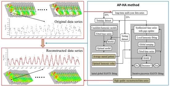
The AP-HA algorithm was mainly designed based on the principles of conventional HANTS algorithms [29]. Two main innovate strategies were developed to improve the reconstruction performance. One strategy involves model selection based on the cross-validation method, which adaptively chooses the optimal harmonic formula. The other strategy is an iterative piecewise fitting procedure, which aims to better track the short-term intra-annual variations and long-term inter-annual fluctuations. In the following, we describe the main steps of the AP-HA implementation using the flowchart shown in Figure 1.
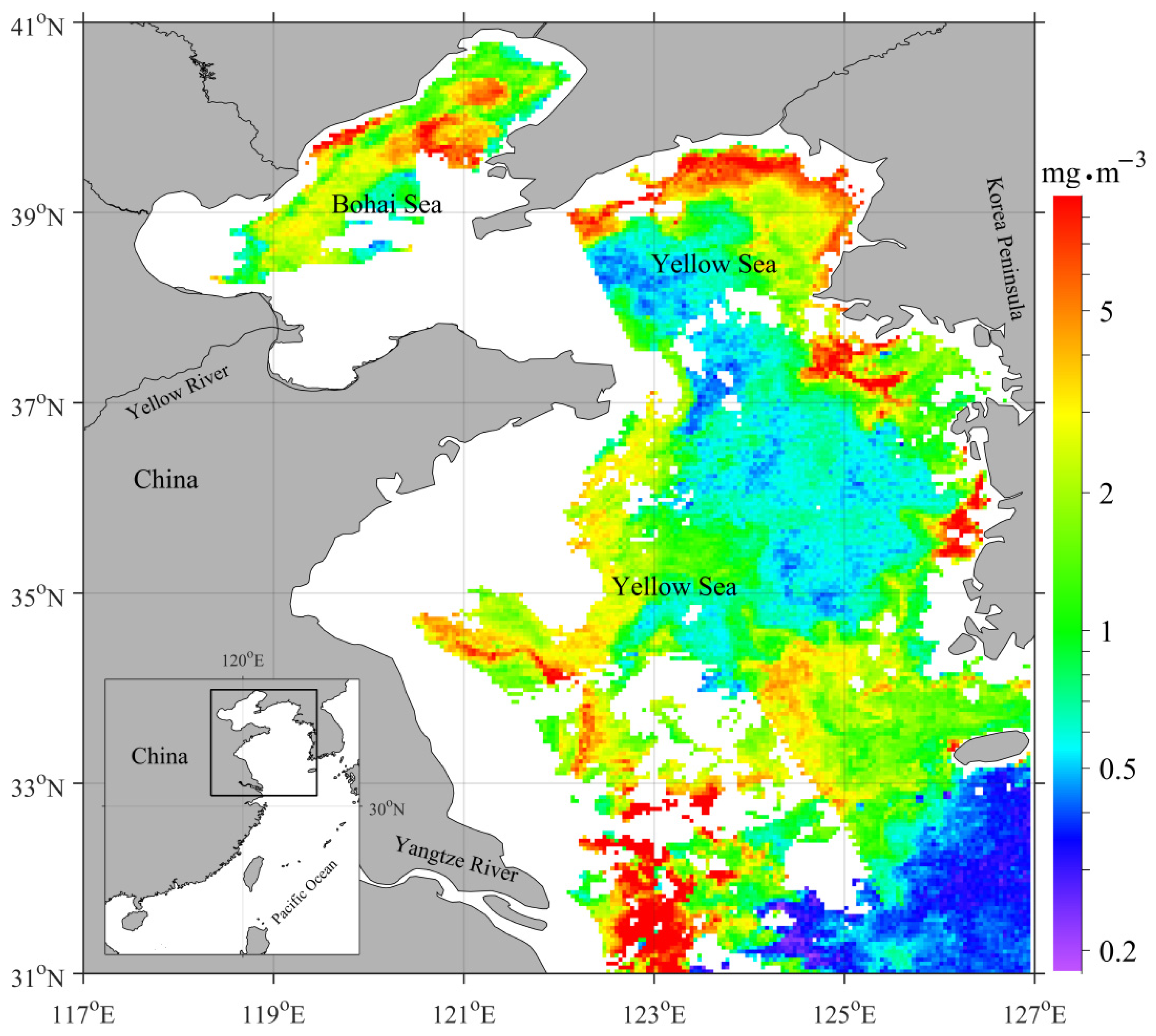
2.2.1. Step 1: Preprocessing of the Original Data Series
The original data series of a pixel contains both existing and missing observations. Before reconstruction, 20% of the existing observations in the target data series were randomly selected as the testing dataset and the remaining 80% of the existing observations were the training dataset. The training dataset was mainly used for model fitting, while the testing dataset was used for progressive cross-validation of the fitted results.
2.2.2. Step 2: Initial Global HANTS Fitting
In this step, a global HANTS fitting process (shown in Equation (1)) was preliminarily carried out on the training dataset to construct a simple average annual model for the target data series (see Figure 1). Here, both the maximum of the polynomial degree (L in Equation (1)) and the harmonic order (N in Equation (1)) were set in the range of 0 to 13, which resulted in a total of 196 candidate models. The optimal harmonic formula was determined through cross-validation as the one with the minimum RMSE (root mean squared error) values between the fitted and original values over the testing dataset. The established global harmonic model serves a two-fold purpose. First, it provides an initial estimate of missing observations in the data series, particularly for extensive continuous data gaps, which might generate spurious artifacts in the progressive harmonic fitting procedure [30]. Second, the harmonic order of the global harmonic model can be used for the iterative piecewise fitting procedure, as demonstrated in step 3. As a result, a new cloud-free data series was synthesized by integrating raw values of existing data points with prefilled values of missing data points. Specifically, the existing observations in the training dataset were kept as their original values, while the values for gaps were prefilled by the initial global harmonic model in this step.
2.2.3. Step 3: Iterative Piecewise HANTS Fitting
To better account for local intra-annual and inter-annual traits in the multi-year data series, the piecewise fitting approach could be a potential scheme solution, as proposed in AG and DL methods [23]. When AG and DL methods are applied on long-term data series with multiple cycles, the entire data series are first divided into successive subseries according to the peaks and troughs, then each subseries is individually fitted and finally merged into a global data series. As a consequence, AG and DL methods, which primarily extract the locations of peaks and troughs in the data series, are necessary but time-consuming; however, for harmonic function, it is not necessary to divide the long-term time series around the local peak or trough, as is the case with AG and DL methods. Here, we simply divided the original data record into multiple annual subseries with one year step from the first observation. We then fit a HANTS model consisting of a constant and fixed harmonic order (as the harmonic order of the initial global harmonic model in step 2) to each subseries. A global function could then be merged using the weighted average method.
The local piecewise fitting and subsequent global merging scheme is illustrated in Figure 2 with an example time series. Specifically, the predefined HANTS function was successively fitted to each subseries, resulting in a series of local functions, then the curve of each overlapped segment was merged with the two adjacent local functions. In general, the global functions (Yr*) can be calculated as:
where Yr1 and Yr2 are the local functions of subseries from T1 to T3 and T2 to T4, respectively; α is the weight of each observation.
In fact, the average annual pattern constructed by the global HANTS fitting algorithm in step 2 is not strictly equivalent to the actual profile during a specific year, which might result in unrealistic biases between piecewise fitted values (obtained in step 3) and the original values of existing observations. In order to make the fitted values approach the original values of existing observations as closely as possible, an iterative fitting process based on the cross-validation was designed. After the first piecewise fitting process, the training dataset was updated, with the missing observations being replaced by the new fitted values, then the RMSE between the original and piecewise fitted values for the testing dataset was calculated and recorded. Then, we ran another piecewise fitting procedure on the updated training time series and calculated the RMSE for the testing time series from the new piecewise fitted values. This process iterates as the RMSE gradually decreases. The iterations stop when the RMSE starts to increase, then the final reconstructed data series can be obtained as the piecewise fitted data series from the last iteration, which will have the lowest RMSE value (see Figure 1).
2.3. Evaluation Strategy
The main objective of this study was to construct an improved version of the conventional HANTS algorithms to achieve greater accuracy and to allow adaptive optimization when applied for multi-year time series reconstruction; therefore, to assess the performance of the AP-HA method, it was directly compared with conventional HANTS approaches, which are generally implemented with empirical parameters (i.e., polynomial degree and harmonic order). In this study, the candidate HANTS models were HA31, HA53, HA75 and HA97, with polynomial degrees (L in Equation (1)) and harmonic orders (N in Equation (1)) set to 3 and 1, 5 and 3, 7 and 5 and 9 and 7, respectively. HA-CV refers to the initial global HANTS model obtained through cross-validation in step 2. As stated in Section 2.2.1, the original dataset was randomly divided into training and testing datasets. The root mean square error (RMSE) between the fitted values and original values for the testing dataset was used for quantitative evaluation. Visual inspections of temporal and spatial variations in the reconstructed and original data series and images were used for qualitative evaluation.
2.4. Sea Surface Chlorophyll-a Dataset
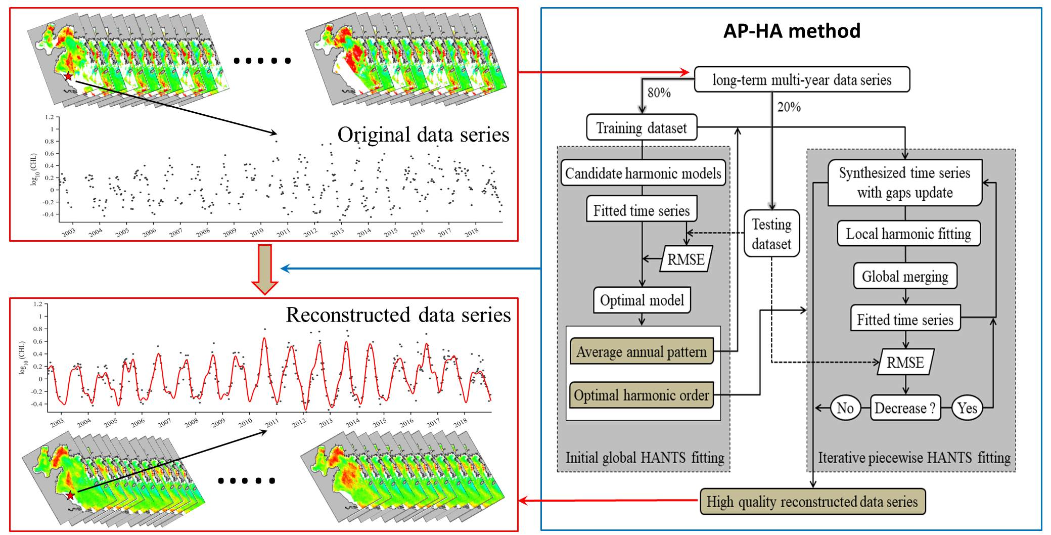
In this study, the weekly composite satellite-derived sea surface chlorophyll-a (CHL) data over the Bohai and Yellow Seas (BYS) of China (Figure 3) were employed to examine and compare the performance of the candidate reconstruction techniques. Level 2 daily remote sensing reflectance (Rrs) images from the moderate-resolution imaging spectroradiometer (MODIS) on the Aqua satellite with local area coverage (LAC) during the period from 4 July 2002 to 31 December 2018 were downloaded for the geographic area of 117–127°E by 31–41°N from the OceanColor website of the Goddard Space Flight Center (http://oceancolor.gsfc.nasa.gov/). The daily Rrs images were remapped onto a common 1/24° × 1/24° grid based on linear interpolation for convenience and to reduce the data volume for data analysis. A regional statistical GAM (generalized additive model) algorithm was used to calculate the daily sea surface CHL based on Rrs datasets, which have improved accuracy in both magnitude and seasonality when compared with the standard OC3M (ocean CHL three-band algorithm for MODIS) algorithm [33]. The daily CHL images were merged to weekly images using median values, and finally a weekly composite dataset with 240 × 240 spatial pixels and 858 temporal steps (with 52 steps in a complete year) spanning from July 2002 to December 2018 was constructed for further analysis. The weekly composite CHL dataset contained lots of missing observations, with a total percentage of 63.6%. The temporal profiles of sea surface CHL in this area are mainly governed by periodic seasonal patterns and can theoretically be fitted with a series of harmonics [34,35]. Therefore, the harmonic-based algorithms could be used to simulate and reconstruct CHL time series; however, due to their log-normal distribution characteristic, the CHL values should be log-transformed (on the base of 10) before all analyses [36].
3. Results
The AP-HA method and other candidate methods were applied to the CHL dataset pixel-by-pixel to reconstruct long-term complete data series of each pixel. In this section, the AP-HA method was first illustrated on a selected CHL time series as an example. Then, the reconstruction performance of all methods was quantitatively evaluated and visually inspected.
3.1. Illustrating the AP-HA Implementation on a Profile
The panels in Figure 4 illustrate the results for each step in the AP-HA algorithm when implemented on a selected CHL time series. Following the AP-HA algorithm, the original data series was randomly divided into training data series and testing data series with percentages of 80% and 20%, respectively (Figure 4a). Then, the global HANTS fitting was applied on the training data series to acquire its average annual model. Through cross-validation based on the testing data series, the optimal average model was constructed with the 9th-order polynomial and 3rd-order harmonic, as shown in Figure 4b. Using the average annual model, the missing values in the training data series were roughly filled, which resulted in an updated training data series without gaps. Then, the iterative piecewise fitting procedure was applied on the new training data series to produce multiple fitted data series, which gradually converged to the final reconstructed data series after 8 iterations, giving the minimum RMSE for the testing data series (Figure 4c). The reconstructed data series reproduced the seasonal patterns quite well and better tracked the traits of intra-annual and inter-annual variations (Figure 4c).
3.2. Overall Quantitative Evaluation
Table 1 presents the RMSE values for the candidate methods over the training and testing datasets, respectively. Among the conventional HANTS methods, the RMSE values of the training dataset continuously decreased with increased harmonic orders in the models, which confirmed that the higher harmonic orders in HANTS better approach the original observations [28]. In contrast, based on the independent testing dataset, the HA53 method achieved the lowest RMSE value of the conventional HANTS methods. These results indicate that the parameters (i.e., the polynomial degree and harmonic order) of the HANTS models should be appropriately defined in order to obtain the best performance for the purpose of reconstructing missing data. The AP-HA method clearly exhibited the best performance out of the two datasets (i.e., training dataset and testing dataset), as indicated by having the lowest RMSE values for the testing dataset. In addition, the lower RMSE achieved by the HA-CV method than by the four conventional methods indicates the effectiveness of cross-validation in improving the reconstruction accuracy. The iterative piecewise fitting further improved the accuracy, as indicated by the lower RMSE of the AP-HA method than that of the HA-CV method.
3.3. Visual Inspection of Typical Data Series
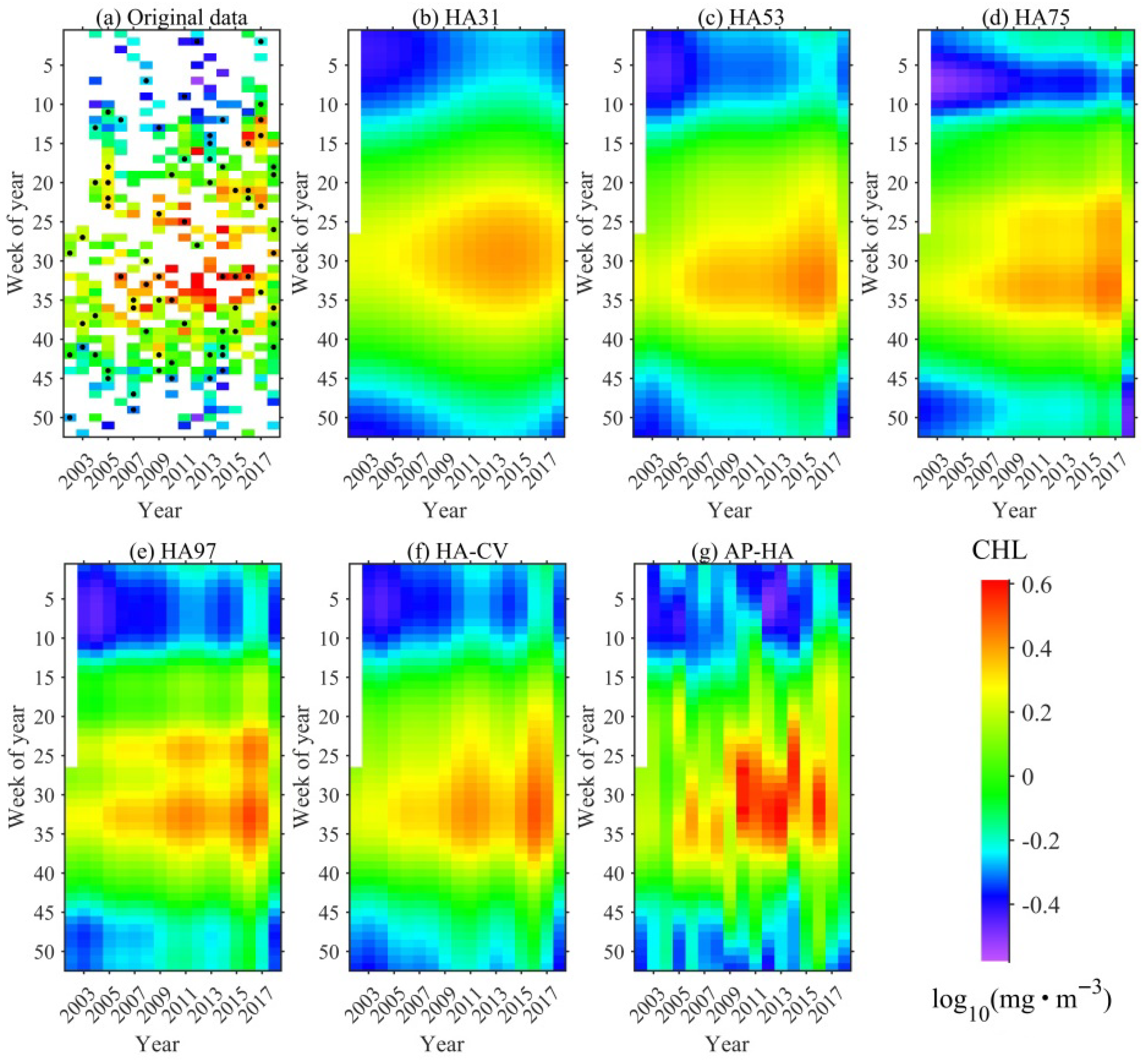
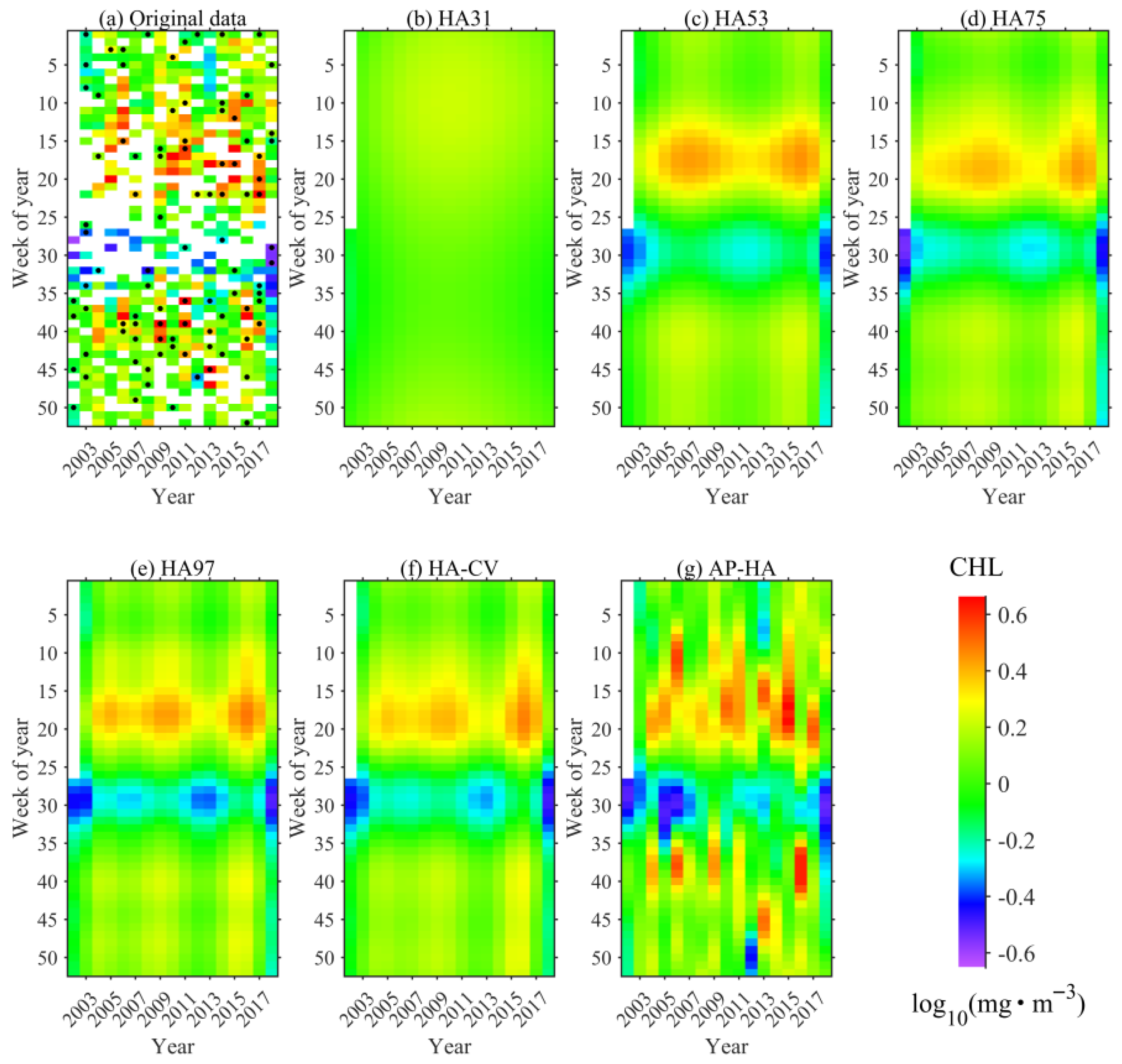
The multi-year CHL time series reconstructed by candidate methods were plotted against different years in order to visually compare their capabilities in tracking the intra-annual and inter-annual traits of the original time series. Two original CHL time series associated with the reconstructed profiles are given as examples in Figure 5 and Figure 6. Figure 5 presents a typical CHL profile with a unimodal annual pattern, while Figure 6 presents a typical CHL profile with a bimodal annual pattern. As Figure 5 shows, all methods did well in reproducing the average seasonal pattern with a single peak in summer and a single trough during winter; however, the reconstructed profiles using conventional methods appeared to be too stiff to track the fine structure of the data series, and were particularly unresponsive to the transient changes in the data series (Figure 5b–f). In comparison, the AP-HA profiles exhibited the best representation of the detail traits of the original data series, capturing the peak and trough values particularly well. In a quantitative assessment, the AP-HA method achieved the highest accuracy with a 9th-order polynomial and 3rd-order harmonic (RMSE = 0.134). Even though the same harmonic order was used, the AP-CV still achieved lower accuracy (RMSE = 0.161) than the AP-HA method, demonstrating the benefits of the iterative piecewise fitting scheme in the AP-HA method. For the bimodal pattern shown in Figure 6, the CHL seasonality with two peaks in spring and autumn and two troughs in summer and winter was well reproduced by all techniques. In comparison, the AP-HA profile exhibited the best representation of the detail traits when compared to the original data series, capturing the peaks and trough values particularly well. (Figure 6). Quantitatively speaking, the AP-HA method performed best using the 7th-order polynomial and 5th-order harmonic formula (RMSE = 0.174), while the RMSE values for all other methods were larger than 0.230. In summary, although all methods did well in reproducing the average annual patterns of CHL time series, although the AP-HA exhibited significantly higher capability in reproducing the details of intra-annual and inter-annual variations in multi-year seasonal time series.
3.4. Results of Reconstructed CHL Images
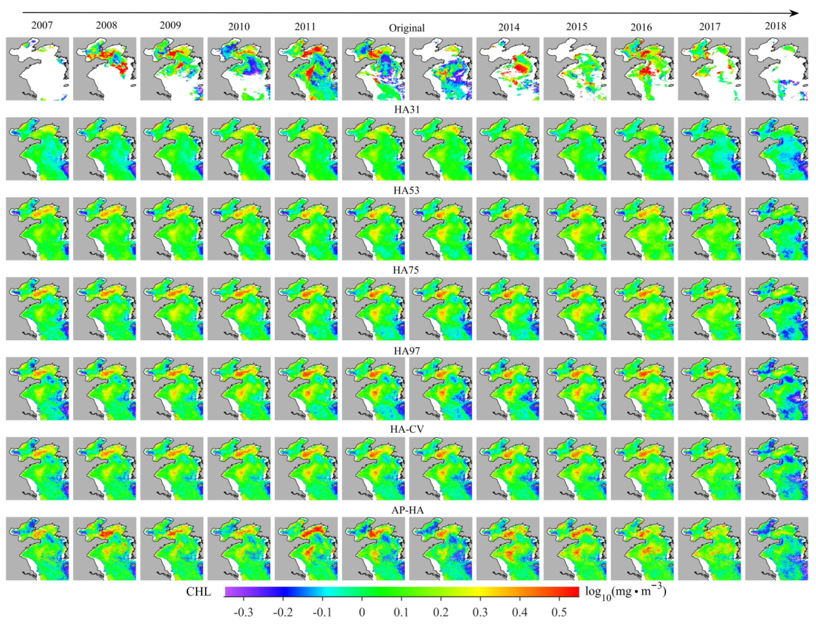
To evaluate and compare the spatial performance of the candidate harmonic-based techniques for CHL data reconstruction, we visually inspected the examples of original CHL and reconstructed images, as shown in Figure 7 and Figure 8. Figure 7 shows an example of a temporal sequence of 12 connected weekly images (13rd‒24th weeks of year 2011), illustrating their ability to track intra-annual traits. Figure 8 shows an example of weekly images for week 13 for different years (week 13 for the years 2007‒2018), emphasizing their inter-annual behaviors. No obvious spatial discontinuity was present in the reconstructed images, demonstrating that all of the methods achieved reasonable spatial patterns, although no spatial information was considered in these methods. As shown in Figure 7, all of the reconstructed images exhibited similar spatial and temporal patterns as the original images; however, the AP-HA method was much better when approaching the high and low values of the original images. As shown in Figure 8, all of the methods did well in delineating the spatial and temporal patterns of the original CHL images, while the AP-HA images better tracked the inter-annual fluctuations of the original CHL images. The results from the image comparison confirmed that all of the candidate harmonic methods did well in tracking the spatial distributions and the average annual patterns, while the proposed AP-HA method better reproduced the detailed intra-annual and inter-annual traits.
4. Discussion
4.1. Improvements in AP-HA Method
We developed an improved harmonic-based fitting approach to reconstruct long-term time series using MODIS satellite-derived weekly CHL data series for the BYS as an example. To our knowledge, this is the first experiment on piecewise harmonic fitting to reconstruct multi-year incomplete data series. As the results show, the AP-HA method was demonstrated to be an adaptive and reliable technique that is capable of reconstructing multi-year CHL time series with various features, including gap distributions and local profiles traits. The improvement of the AP-HA method was mainly due to the following aspects.
First, a preliminary global HANTS fitting method was employed to prefill the missing observations. In fact, various prefilling algorithms had been adopted prior to application of harmonic fitting in previous studies, confirming that the prefilling method is indeed an efficient way to improve accuracy, as well as to promote the stability of the HANTS fitting method, particular for data series with substantial and continuous gaps [19,29,30,37]; however, in this study, we chose the global HANTS algorithm as the prefilling method due to its global nature, ease of implementation and consistency with the next step piecewise in the HANTS fitting method. Although no comparison was made between other prefilling methods reported in previous studies and the HANTS method we used in this study, the results clearly showed that the stated goals of improving the accuracy and maintaining the stability of the harmonic-based algorithms were achieved.
Second, the cross-validation was first introduced as an objective criterion to determine the optimal harmonic formulas in the HANTS fitting method in this study. In practice, the HANTS fitting based on cross-validation RMSE values achieved the ultimate objective of adaptively determining the optimal harmonic model with a combination of polynomial degrees and harmonic orders. As a consequence, the cross-validation scheme was demonstrated to be an effective criterion for optimal model selection in the HANTS algorithm. Furthermore, the iterative process meant the harmonic fitted values gradually approach the detail local traits of the original data series and quantitatively increased the accuracy of the reconstructed results.
In addition, for piecewise-defined AG and DL algorithms, it is essential to identify the local maximum and minimum points in order to segment the complete data series into several subseries [20,23,38]. In contrast, the identification of local maximum and minimum points is not necessary for the harmonic-based functions owing to their flexible nature. For example, in this study, we directly extracted the first subseries from the 1st to the 52th data points, the second subseries from the 27rd to the 78th points, the third subseries from the 79th to the 104th points and so on. From this point of view, the AP-HA method is easy to operate. Furthermore, from an implementation point of view, one cycle of the global HANTS fitting process was able to simultaneously prefill all missing observations, demonstrate its higher efficiency than other local-based prefilling methods.
4.2. Limitations and Perspective
At present, there are no continuous field survey plots in the BYS that can provide concurrent CHL time series information for the study period (2002–2018) that could be used for a direct or an indirect validation of the results from this study; therefore, it is impossible to establish one-to-one relations between the reconstructed values and those measured from field-based observations. In this study, the cross-validation method was adopted to select the best model and to evaluate the reconstructed accuracy. These schemes assumed that the satellite-derived CHL values were unbiased, which is generally not true for optically complex coastal waters such as the BYS. In particular, when a testing dataset contains many noisy observations, the outcome is likely to be highly uncertain. Regardless, for missing data reconstruction purposes, the proposed AP-HA method clearly achieved the stated goals of adaptive parameter selection, robust performance and improved accuracy.
The pixel-wise global HANTS fitting approach to constructing an average annual model provides prefilled values for gaps in any location. The representativeness of the constructed average annual model depends on the inter-annual variability of the time series; that is to say, large inter-annual variability implies a poorer fit of the average annual pattern because the real series generally vary over different years. As such, this method is unsuitable for regions with frequent changes of annual shapes in different years. The method used in this study was performed only on data series of a single pixel; therefore, no spatial coherence was considered, although the reconstructed CHL examples generated using the AP-HA approach were spatially coherent and natural looking (as shown in Figure 7 and Figure 8), demonstrating that temporal information may be adequate for acquiring reliable results using the AP-HA approach.
As a self-adaptive method, the AP-HA method relaxes the constraints on the artificial setting of harmonic orders that occur in conventional HANTS methods, making the implementations more objective; however, several parameters must be predefined before the AP-HA method is implemented, such as the maximum polynomial degree and harmonic order in the initial models. In this respect, further studies are required to solve these issues, or at least to allow a sensitivity analysis of these parameters. Regardless, the AP-HA method is undoubtedly more objective and accurate than the conventional harmonic-based methods. While being substantially more adaptable to a greater variety of practical applications, the AP-HA technique also involves significantly more mathematical overhead owing to the processes involved in optimal model selection and iterative piecewise fitting. In our view, and clearly in the view of others who have previously used such techniques, the added computational effort is well worth the investment.
5. Conclusions
The HANTS method has been widely used in the smoothing and reconstruction of time series. Appropriate modifications to this method could improve its performance for specific applications. In this study, we proposed an adaptive piecewise harmonic-based fitting approach (AP-HA) that can search for the optimal model needed to reconstruct high-quality multi-year cyclic profiles from incomplete satellite data series. By applying the newly developed method to a weekly satellite-derived sea surface CHL product and by comparing the results with those of the conventional HANTS methods, we found that the AP-HA method has the following advantages: (1) the cross-validation process was adopted to choose the optimal parameters in harmonic models, which is more objective than the widely used empirically predetermined method; (2) the iterative piecewise fitting scheme significantly improved the capability of the harmonic models in tracking the intra-annual and inter-annual traits of multiyear time series; (3) the prefilling of missing values using the preliminary global HANTS means the proposed method is suitable for various data gap conditions.
The outputs of the AP-HA are long-term time series without temporal or spatial data gaps. This method is an improvement of the conventional HANTS method for long-term reconstruction, which can effectively restore cyclic patterns of seasonal variables. Although the AP-HA method has only been examined for CHL data in the ocean, due to its nature, this method is expected to be suitable for a wide range of other datasets with cyclic annual patterns.
Author Contributions
Conceptualization, Y.W. and J.N.; methodology, Y.W. and Z.G.; software, Y.W.; formal analysis, Y.W. and J.N.; writing—original draft preparation, Y.W.; writing—review and editing, Y.W., J.N. and Z.G.; funding acquisition, Y.W. All authors have read and agreed to the published version of the manuscript.
Funding
This work was supported by the National Natural Science Foundation of China (grant numbers 41706134 and 42030402), and the Open Fund of the CAS Key Laboratory of Marine Ecology and Environmental Sciences, Institute of Oceanology, Chinese Academy of Sciences (grand number: KLMEES202005).
Acknowledgments
The authors would like to thank the Ocean Biology Processing Group of NASA for providing the MODIS dataset (http://oceancolor.gsfc.nasa.gov/). The authors are thankful to the three anonymous reviewers who contributed to the manuscript with valuable comments.
Conflicts of Interest
The authors declare no conflict of interest.
References
- Piao, S.L.; Fang, J.Y.; Zhou, L.M.; Ciais, P.; Zhu, B. Variations in satellite-derived phenology in China’s temperate vegetation. Glob. Chang. Biol. 2006, 12, 672–685. [Google Scholar] [CrossRef]
- Gregg, W.W.; Conkright, M.E. Decadal changes in global ocean chlorophyll. Geophys. Res. Lett. 2002, 29. [Google Scholar] [CrossRef] [Green Version]
- Gregg, W.W.; Woodward, R.H. Improvements in coverage frequency of ocean color: Combining data from SeaWiFS and MODIS. Trans. Geosci. Remote Sens. 1998, 36, 1350–1353. [Google Scholar] [CrossRef]
- Pottier, C.; Garcon, V.; Larnicol, G.; Sudre, J.; Schaeffer, P.; Le Traon, P.Y. Merging SeaWiFS and MODIS/Aqua ocean color data in North and Equatorial Atlantic using weighted averaging and objective analysis. Trans. Geosci. Remote Sens. 2006, 44, 3436–3451. [Google Scholar] [CrossRef] [Green Version]
- Bai, K.; Chang, N.-B.; Chen, C.-F. Spectral information adaptation and synthesis scheme for merging cross-mission ocean color reflectance observations from MODIS and VIIRS. Trans. Geosci. Remote Sens. 2016, 54, 311–329. [Google Scholar] [CrossRef]
- Zhang, X.Y.; Friedl, M.A.; Schaaf, C.B.; Strahler, A.H.; Hodges, J.C.F.; Gao, F.; Reed, B.C.; Huete, A. Monitoring vegetation phenology using MODIS. Remote Sens. Environ. 2003, 84, 471–475. [Google Scholar] [CrossRef]
- Barale, V.; Jaquet, J.-M.; Ndiaye, M. Algal blooming patterns and anomalies in the Mediterranean Sea as derived from the SeaWiFS data set (1998–2003). Remote Sens. Environ. 2008, 112, 3300–3313. [Google Scholar] [CrossRef]
- Chen, S.; Hu, C. Estimating sea surface salinity in the northern Gulf of Mexico from satellite ocean color measurements. Remote Sens. Environ. 2017, 201, 115–132. [Google Scholar] [CrossRef]
- Demarcq, H.; Reygondeau, G.; Alvain, S.; Vantrepotte, V. Monitoring marine phytoplankton seasonality from space. Remote Sens. Environ. 2012, 117, 211–222. [Google Scholar] [CrossRef]
- Wang, Y.Q.; Gao, Z.Q.; Liu, D.Y. Multivariate DINEOF reconstruction for creating long-term cloud-free chlorophyll-a data records from SeaWiFS and MODIS: A case study in Bohai and Yellow Seas, China. J. Sel. Top. Appl. Earth Obs. Remote Sens. 2019, 12, 1383–1395. [Google Scholar] [CrossRef]
- Liu, X.M.; Wang, M.H. Gap filling of missing data for VIIRS global ocean color products using the DINEOF method. Trans. Geosci. Remote Sens. 2018, 56, 4464–4476. [Google Scholar] [CrossRef]
- Pukhtyar, L.D.; Stanichny, S.V.; Timchenko, I.E. Optimal interpolation of the data of remote sensing of the sea surface. Phys. Oceanogr. 2009, 19, 225–239. [Google Scholar] [CrossRef]
- Cole, H.; Henson, S.; Martin, A.; Yool, A. Mind the gap: The impact of missing data on the calculation of phytoplankton phenology metrics. J. Geophys. Res. Ocean. 2012, 117, C08030. [Google Scholar] [CrossRef]
- Racault, M.-F.; Sathyendranath, S.; Platt, T. Impact of missing data on the estimation of ecological indicators from satellite ocean-colour time-series. Remote Sens. Environ. 2014, 152, 15–28. [Google Scholar] [CrossRef] [Green Version]
- Ferreira, A.S.; Visser, A.W.; MacKenzie, B.R.; Payne, M.R. Accuracy and precision in the calculation of phenology metrics. J. Geophys. Res. Ocean. 2014, 119, 8438–8453. [Google Scholar] [CrossRef]
- Jönsson, P.; Cai, Z.; Melaas, E.; Friedl, M.A.; Eklundh, L. A method for robust estimation of vegetation seasonality from Landsat and Sentinel-2 time series data. Remote Sens. 2018, 10, 635. [Google Scholar] [CrossRef] [Green Version]
- Zeng, L.; Wardlow, B.D.; Xiang, D.; Hu, S.; Li, D. A review of vegetation phenological metrics extraction using time-series, multispectral satellite data. Remote Sens. Environ. 2020, 237, 111511. [Google Scholar] [CrossRef]
- Wasmund, N.; Nausch, G.; Gerth, M.; Busch, S.; Burmeister, C.; Hansen, R.; Sadkowiak, B. Extension of the growing season of phytoplankton in the western Baltic Sea in response to climate change. Mar. Ecol. Prog. Ser. 2019, 622, 1–16. [Google Scholar] [CrossRef] [Green Version]
- Yan, L.; Roy, D.P. Spatially and temporally complete Landsat reflectance time series modelling: The fill-and-fit approach. Remote Sens. Environ. 2020, 241, 111718. [Google Scholar] [CrossRef]
- Hermance, J.F.; Jacob, R.W.; Bradley, B.A.; Mustard, J.F. Extracting phenological signals from multiyear AVHRR NDVI time series: Framework for applying high-order annual splines with roughness damping. Trans. Geosci. Remote Sens. 2007, 45, 3264–3276. [Google Scholar] [CrossRef]
- Chen, J.; Jonsson, P.; Tamura, M.; Gu, Z.H.; Matsushita, B.; Eklundh, L. A simple method for reconstructing a high-quality NDVI time-series data set based on the Savitzky-Golay filter. Remote Sens. Environ. 2004, 91, 332–344. [Google Scholar] [CrossRef]
- Atzberger, C.; Eilers, P.H.C. A time series for monitoring vegetation activity and phenology at 10-daily time steps covering large parts of South America. Int. J. Digit. Earth 2011, 4, 365–386. [Google Scholar] [CrossRef]
- Jonsson, P.; Eklundh, L. Seasonality extraction by function fitting to time-series of satellite sensor data. Trans. Geosci. Remote Sens. 2002, 40, 1824–1832. [Google Scholar] [CrossRef]
- Jakubauskas, M.E.; Legates, D.R.; Kastens, J.H. Harmonic analysis of time-series AVHRR NDVI data. Photogramm. Eng. Remote Sens. 2001, 67, 461–470. [Google Scholar]
- Atkinson, P.M.; Jeganathan, C.; Dash, J.; Atzberger, C. Inter-comparison of four models for smoothing satellite sensor time-series data to estimate vegetation phenology. Remote Sens. Environ. 2012, 123, 400–417. [Google Scholar] [CrossRef]
- Cai, Z.Z.; Jonsson, P.; Jin, H.X.; Eklundh, L. Performance of smoothing methods for reconstructing NDVI time-series and estimating vegetation phenology from MODIS data. Remote Sens. 2017, 9, 1271. [Google Scholar] [CrossRef] [Green Version]
- Liu, R.G.; Shang, R.; Liu, Y.; Lu, X.L. Global evaluation of gap-filling approaches for seasonal NDVI with considering vegetation growth trajectory, protection of key point, noise resistance and curve stability. Remote Sens. Environ. 2017, 189, 164–179. [Google Scholar] [CrossRef] [Green Version]
- Zhou, J.; Jia, L.; Menenti, M. Reconstruction of global MODIS NDVI time series: Performance of Harmonic ANalysis of Time Series (HANTS). Remote Sens. Environ. 2015, 163, 217–228. [Google Scholar] [CrossRef]
- Hermance, J.F. Stabilizing high-order, non-classical harmonic analysis of NDVI data for average annual models by damping model roughness. Int. J. Remote Sens. 2007, 28, 2801–2819. [Google Scholar] [CrossRef]
- Padhee, S.K.; Dutta, S. Spatio-Temporal reconstruction of MODIS NDVI by regional land surface phenology and harmonic analysis of time-series. GISci. Remote Sens. 2019, 56, 1261–1288. [Google Scholar] [CrossRef]
- Huan, Y.; Sun, D.; Wang, S.; Zhang, H.; Qiu, Z.; Bilal, M.; He, Y. Remote sensing estimation of phytoplankton absorption associated with size classes in coastal waters. Ecol. Indic. 2021, 121, 107198. [Google Scholar] [CrossRef]
- Moore, T.S.; Brown, C.W. Incorporating environmental data in abundance-based algorithms for deriving phytoplankton size classes in the Atlantic Ocean. Remote Sens. Environ. 2020, 240, 111689. [Google Scholar] [CrossRef]
- Wang, Y.Q.; Liu, D.Y.; Tang, D.L. Application of a generalized additive model (GAM) for estimating chlorophyll-a concentration from MODIS data in the Bohai and Yellow Seas, China. Int. J. Remote Sens. 2017, 38, 639–661. [Google Scholar] [CrossRef]
- Vargas, M.; Brown, C.W.; Sapiano, M.R.P. Phenology of marine phytoplankton from satellite ocean color measurements. Geophys. Res. Lett. 2009, 36, L01608. [Google Scholar] [CrossRef] [Green Version]
- Wang, Y.Q.; Gao, Z.Q. Contrasting chlorophyll-a seasonal patterns between nearshore and offshore waters in the Bohai and Yellow Seas, China: A new analysis using improved satellite data. Cont. Shelf Res. 2020, 203. [Google Scholar] [CrossRef]
- Campbell, J.W. The lognormal distribution as a model for bio-optical variability in the sea. J. Geophys. Res. 1995, 100, 13237–13254. [Google Scholar] [CrossRef]
- Bradley, B.A.; Jacob, R.W.; Hermance, J.F.; Mustard, J.F. A curve fitting procedure to derive inter-annual phenologies from time series of noisy satellite NDVI data. Remote Sens. Environ. 2007, 106, 137–145. [Google Scholar] [CrossRef]
- Yang, Y.; Luo, J.; Huang, Q.; Wu, W.; Sun, Y. Weighted double-logistic function fitting method for reconstructing the high-quality sentinel-2 NDVI time series data set. Remote Sens. 2019, 11, 2342. [Google Scholar] [CrossRef] [Green Version]
Figure 1.
Flowchart showing the reconstruction process of a time series using the AP-HA method.

Figure 2.
Graphical illustration of the two successive local fittings and their merging. Yr1 and Yr2 are the two local harmonic functions from T1 to T3 and T2 to T4, respectively. Yr* is their merged function for the overlapped period from T2 to T3.
Figure 2.
Graphical illustration of the two successive local fittings and their merging. Yr1 and Yr2 are the two local harmonic functions from T1 to T3 and T2 to T4, respectively. Yr* is their merged function for the overlapped period from T2 to T3.

Figure 3.
Location of the study area overlaid with a composite image of satellite-derived sea surface chlorophyll-a concentrations during 10–16 September 2013.
Figure 3.
Location of the study area overlaid with a composite image of satellite-derived sea surface chlorophyll-a concentrations during 10–16 September 2013.

Figure 4.
Example of a CHL time series and the outputs in the different steps of the proposed AP-HA method. Data series result from the three steps: (a) preprocessing of the original data series; (b) initial global HANTS fitting; (c) iterative piecewise HANTS fitting.
Figure 4.
Example of a CHL time series and the outputs in the different steps of the proposed AP-HA method. Data series result from the three steps: (a) preprocessing of the original data series; (b) initial global HANTS fitting; (c) iterative piecewise HANTS fitting.

Figure 5.
Example of an original unimodal CHL time series associated with the reconstructed time series, which was processed using different methods: (a) original method; (b) HA31; (c) HA53; (d) HA75; (e) HA97; (f) HA-CV; (g) AP-HA. (a) The points indicate testing data being selected.
Figure 5.
Example of an original unimodal CHL time series associated with the reconstructed time series, which was processed using different methods: (a) original method; (b) HA31; (c) HA53; (d) HA75; (e) HA97; (f) HA-CV; (g) AP-HA. (a) The points indicate testing data being selected.

Figure 6.
Example of an original bimodal CHL time series associated with the reconstructed time series, which was processed using different methods: (a) original method; (b) HA31; (c) HA53; (d) HA75; (e) HA97; (f) HA-CV; (g) AP-HA. (a) The points indicate testing data being selected.
Figure 6.
Example of an original bimodal CHL time series associated with the reconstructed time series, which was processed using different methods: (a) original method; (b) HA31; (c) HA53; (d) HA75; (e) HA97; (f) HA-CV; (g) AP-HA. (a) The points indicate testing data being selected.

Figure 7.
Time series of weekly CHL images for weeks 13 to 24 for the year 2011.

Figure 8.
Time series of weekly CHL images for week 13 for different years.


Table 1.
Statistics for the RMSE values for the candidate HANTS methods.
| Dataset | HA31 | HA53 | HA75 | HA97 | HA-CV | AP-HA |
|---|---|---|---|---|---|---|
| Training | 0.224 | 0.198 | 0.192 | 0.188 | 0.195 | 0.155 |
| Testing | 0.229 | 0.207 | 0.281 | 0.303 | 0.197 | 0.188 |
Publisher’s Note: MDPI stays neutral with regard to jurisdictional claims in published maps and institutional affiliations. |
© 2021 by the authors. Licensee MDPI, Basel, Switzerland. This article is an open access article distributed under the terms and conditions of the Creative Commons Attribution (CC BY) license (https://creativecommons.org/licenses/by/4.0/).
Share and Cite
MDPI and ACS Style
Wang, Y.; Gao, Z.; Ning, J. An Adaptive Piecewise Harmonic Analysis Method for Reconstructing Multi-Year Sea Surface Chlorophyll-A Time Series. Remote Sens. 2021, 13, 2727. https://0-doi-org.brum.beds.ac.uk/10.3390/rs13142727
AMA Style
Wang Y, Gao Z, Ning J. An Adaptive Piecewise Harmonic Analysis Method for Reconstructing Multi-Year Sea Surface Chlorophyll-A Time Series. Remote Sensing. 2021; 13(14):2727. https://0-doi-org.brum.beds.ac.uk/10.3390/rs13142727
Chicago/Turabian StyleWang, Yueqi, Zhiqiang Gao, and Jicai Ning. 2021. "An Adaptive Piecewise Harmonic Analysis Method for Reconstructing Multi-Year Sea Surface Chlorophyll-A Time Series" Remote Sensing 13, no. 14: 2727. https://0-doi-org.brum.beds.ac.uk/10.3390/rs13142727
Note that from the first issue of 2016, this journal uses article numbers instead of page numbers. See further details here.