Article

Sentinel-1 Time Series for Crop Identification in the Framework of the Future CAP Monitoring

1
Agriculture, Territory and Technologies Integration Unit, Production in Agriculture Department, Walloon Agricultural Research Centre, rue de Liroux 9, 5030 Gembloux, Belgium
2
Earth and Life Institute, Université Catholique de Louvain, Croix du Sud 2, 1348 Louvain-la-Neuve, Belgium
*
Author to whom correspondence should be addressed.
These authors contributed equally to this work and should be considered as co-first authors.
Remote Sens. 2021, 13(14), 2785; https://0-doi-org.brum.beds.ac.uk/10.3390/rs13142785
Submission received: 31 May 2021 / Revised: 2 July 2021 / Accepted: 12 July 2021 / Published: 15 July 2021

Abstract

:
In this upcoming Common Agricultural Policy (CAP) reform, the use of satellite imagery is taking an increasing role for improving the Integrated Administration and Control System (IACS). Considering the operational aspect of the CAP monitoring process, the use of Sentinel-1 SAR (Synthetic Aperture Radar) images is highly relevant, especially in regions with a frequent cloud cover, such as Belgium. Indeed, SAR imagery does not depend on sunlight and is barely affected by the presence of clouds. Moreover, the SAR signal is particularly sensitive to the geometry and the water content of the target. Crop identification is often a pre-requisite to monitor agriculture at parcel level (ploughing, harvest, grassland mowing, intercropping, etc.) The main goal of this study is to assess the performances and constraints of a SAR-based crop classification in an operational large-scale application. The Random Forest object-oriented classification model is built on Sentinel-1 time series from January to August 2020 only. It can identify crops in the Walloon Region (south part of Belgium) with high performance: 93.4% of well-classified area, representing 88.4% of the parcels. Among the 48 crop groups, the six most represented ones get a F1-score higher or equal to 84%. Additionally, this research documents how the classification performance is affected by different parameters: the SAR orbit, the size of the training dataset, the use of different internal buffers on parcel polygons before signal extraction, the set of explanatory variables, and the period of the time series. In an operational context, this allows to choose the right balance between classification accuracy and model complexity. A key result is that using a training dataset containing only 3.2% of the total number of parcels allows to correctly classify 91.7% of the agricultural area. The impact of rain and snow is also discussed. Finally, this research analyses how the classification accuracy depends on some characteristics of the parcels like their shape or size. This allows to assess the relevance of the classification depending on those characteristics, as well as to identify a subset of parcels for which the global accuracy is higher.

Graphical Abstract

1. Introduction

As part of the upcoming reform of the Common Agricultural Policy (CAP) to be implemented from 1 January 2023, the European Commission (EC) has adopted new rules that will allow to increase the use of modern technologies during verifications related to the area-based CAP payments. The legal and technical framework to make use of the advantages of Earth Observation data in the context of CAP controls was provided in 2018 by the EC. In particular, this covers data coming from the EU’s Copernicus Sentinel satellites.
The actual On-the-Spot-Checks (OTSC) control system is based on a yearly verification done by each EU Member State, who must carry out controls on at least 5% of the farms applying for subsidies. The OTSC are fulfilled either by visiting farms, by interpreting Remote Sensing images or combining both methods (RS imagery and rapid field visits on farms). This system will be replaced by a new monitoring approach (Area Monitoring System—AMS), which is a procedure of regular observation, tracking, and assessment of all eligibility criteria, commitments, and other obligations which can be monitored in a continuous way (for instance by using mainly Copernicus Sentinel satellites images).
This allows to move from an a posteriori control to a continuous assessment of a parcel eligibility. The goal is to warn the farmers in due time about a possible detected discrepancy, in order to avoid penalties. For example, in the case of an activity that must be completed before a given date (such as grass mowing), if it has not been performed approaching the deadline, the farmer could be informed that he should ensure compliance before the deadline to avoid a sanction. This will guarantee that farmers are able to carry out their environmental and other obligations in due time and avoid penalties for non-compliance with CAP rules. Reducing the number of farm visits will also significantly decrease the time spent by farmers with inspectors in the field. This new approach also aims at encouraging farmers to benefit from digital technologies, such as crop monitoring at parcel level, to improve agronomic performances while reducing fertilizer costs and environmental impacts.
In this context of agriculture monitoring by remote sensing, accurate and up-to-date crop type maps are a prerequisite for agriculture practices analyses, such as ploughing or harvest detection. Moreover, identification of land cover types provides basic information for generation of other thematic maps and establishes a baseline for monitoring activities.
High temporal and high spatial resolution remote sensing imagery provides a major asset to monitor agriculture and identify crop types. Satellite image crop classifications are mostly obtained from optical imagery [1,2,3,4,5,6,7]. Indeed, surface reflectances are often key explanatory variables for land cover classification [8,9] as well as indices derived from reflectance data, such as the NDVI, NDWI, and Brightness [8,10,11,12,13]. Temporal metrics derived from time series indices have also been used in several studies [8,11,14,15,16]. However, clouds and cloud shadows remain a major challenge for optical time series, as they lead to gaps and missing data. Furthermore, the reliance of operational applications on cloud-free optical images is a critical issue when precise timeliness is strictly required. The cropland mapping methods applied to time series images have proven to perform better than single-date mapping methods [17]. Indeed, as the phenological status of different crop types evolves differently with time, having information over time allows to better discriminate the crops. Therefore, the use of optical data over large and cloudy areas involves working with composite images (including sometimes spatiotemporal context for residual missing pixels in composite images [18,19]), linearly temporally gap-filled images [20], or pixel-wise weighted least-squares smoothing of the values over time [21,22].
The advantages of SAR images allow meeting the rigid data requirements of operational crop monitoring in the CAP policy context. Unlike optical data, SAR images are not affected by the presence of clouds or haze. The SAR sensors can obtain data during both day and night [23]. As a result, temporal series of high spatial resolution can be regularly and reliably recorded throughout a growing season, whereas optical acquisition is never guaranteed. Agricultural crop mapping performs better with regular information during the whole growing season. Another reason to use microwaves is that they can penetrate more deeply into vegetation than optical wavelengths. SAR signal is very sensitive to plant water content. Polarized microwaves respond differently to shapes and orientations of scattering elements of the plant canopy. Such interactions lead to differences both in the backscattered power in those different polarizations and in the degree of penetration through the canopy. Moreover, the Sentinel-1 sensors present a high temporal resolution and a dual-polarization mode.
Before the launch of Sentinel-1, a number of research works have been carried out to use satellite radar images for crop classification, with different bands of acquisition—L-band [24,25], C-band [24,26,27] (and different polarizations), VV, HH, and HV [27]. The C-band Sentinel-1 SAR data have been analyzed temporally to recognize which agricultural crops grow in fields [28,29,30,31,32,33,34]. In [32], the authors classified 14 crop types in Denmark from SAR Sentinel-1 data time series with an average pixel-base accuracy of 86%.
Studies combining both optical and SAR sensors showed that the synergistic use of radar and optical data for crop classification led to richer information increasing classification accuracies compared to optical-only classification [22,35,36,37,38]. In [39], the authors used a deep learning-based architecture for crop classification using Landsat-8 and Sentinel-1 data and obtained accuracies of more than 85% for five major crops.
While other initiatives already used Sentinel-1 data to classify crops, the main innovation of this research is to highlight which choices lead to the crop map with the highest quality, while discussing the constraints associated to them (e.g., using a longer period implies that the crop map is only available later in the year). This allows to choose the right balance between classification accuracy and the operational interest of keeping the model simple. More specifically, this study documents the effects on the classification performance of different choices that can be made for five parameters: the SAR orbit(related to Ascending or Descending modes), the set of explanatory variables, the quality and size of the training sample, the use of different internal buffers on parcel polygons before SAR signal extraction, and the selected period of the time series.
In order to compare the different models, a statistical analysis is conducted to assess whether the performance differences are significant or solely due to the random fluctuations in the results.
The presence of rain or snow during SAR acquisitions, which is a major constraint of using a SAR dataset, is also discussed. Finally, this research analyses how the classification accuracy depends on some characteristics of the parcels such as their size, shape, and classification confidence level. This allows to assess whether the classification of a parcel is relevant depending on that characteristic (e.g., is the classification relevant for small parcels). Furthermore, considering a threshold on those characteristics allows to identify a subset of the parcels for which the global classification accuracy is higher.

2. Materials and Methods

The study is carried out in the context of the preparation by the Walloon region of their implementation of the Area Monitoring System. The cloud frequency in Belgium is quite significant, and the availability of cloud free image time series over the growing season can be a challenge.
This section first presents the study area and the data used for this research. The data used include the Land Parcel Identification System (LPIS) and the Sentinel-1 images. Then, the method is developed.

2.1. Study Area

The Walloon Region (WR) is located in the south part of Belgium (in grey on Figure 1) and covers 16,901 square kilometers.
In this region, agricultural land represents about half of the total area. As shown on Figure 1, the WR is covered by several Sentinel-1 orbits (see below for details), out of which only two will be used in the present study: 37—Descending and 161—Ascending.
Because those two orbits will be compared and used together, only the part of the WR that is covered by both orbits is considered in the study. It corresponds to the hatched part on Figure 1, which is our study area.

2.2. Data

2.2.1. Land Parcel Identification System (LPIS)

The Land Parcel Identification System (LPIS) was designed as the main instrument for the implementation of the CAP’s first pillar, whereby direct payments are made to the farmer once the land and area eligible for payments have been identified and quantified.
The Walloon LPIS is maintained and updated each year using aerial orthoimages with a spatial resolution of 25 cm. In the context of the CAP, applicants use the LPIS and available RS image to indicate the location of the parcels and the total area under cultivation of a particular crop. In the WR, the farmers do the applications online. The LPIS includes a shapefile with polygons representing the delineation of the parcels as declared by the farmers each year. The declared crop must correspond to the crop type present on field on the 31st of May of each delineated plot. In this study, the 2020 LPIS is used.
At the WR level, the farmers 2020 declarations contain 285,776 parcels, which cover a total area of approximately 764,000 hectares. Only 269,278 parcels, referred as “agricultural field” used for food or feed production and covering 742,173 ha, are considered. Among the discarded parcels, one finds for instance fields that are managed for horticulture or environmental concern only, such as ornamental crops or 6 m wide grassed headlands along watercourses. For this study we considered the part of the WR covered by both orbits 37 and 161, which contains 211,875 agricultural fields and covers 617,077 hectares.
The crop types of the same family (e.g., grain maize and fodder maize) are clustered into different crop groups. These groups were defined by the Walloon authorities in the context of the greening of the CAP in 2013. The selected parcels located in the study area represent 48 crop groups. These 48 crop groups exclude the crop groups with less than 7 occurrences (as consequence 18 agricultural fields with exceedingly rare crop types were not included).
The most represented agricultural groups in our study area are grassland, winter wheat, maize, potato, and sugar beet, as detailed on Table 1.

2.2.2. Sentinel-1 Images-Backscattering Coefficient Time Series (8 Months from January until August 2020)

The Sentinel-1 mission is composed of a constellation of two identical satellites performing C-band Synthetic Aperture Radar (SAR) imaging at 5.6 GHz (5.4 cm wavelength), with an effective revisit time of 12 days (6 days considering both satellites).
Interferometric Wide Swath (IW) Mode is the main operational mode over land and features a 5-by-20-metre spatial resolution and a 250 km swath. The level 1 products made up of Single Look Complex (SLC) and Ground Range-Detected (GRD) outputs in single (HH or VV) or double (HH + HV or VV + VH) polarization.
Four different Sentinel-1 orbits (two descending and two ascending) are covering the majority of the WR area. The hours of acquisition are around 5:30 p.m. and 6:00 a.m. (UTC) for Ascending and Descending orbits, respectively. In order to quantify the impact of different local incidence angle and acquisition time for this study, we considered only data coming from one Ascending orbit (161) and one Descending orbit (37).
GRD products (resolution of 20 × 22 m) are pre-processed to obtain calibrated, geo-coded backscattering coefficients sigma nought (σ0) using the European Space Agency’s SNAP Sentinel-1 toolbox software. The GRD SAR data pre-processing chain include geometric and radiometric calibration, with correction for the local incidence angle, using the Shuttle Radar Topography Mission (STRM 90) digital elevation model (DEM). The images are interpolated at a 6.5 × 6.5 m pixel size during the projection in the UTM-31N coordinate system. The 6.5 m pixel size was considered in order to include in our data set a maximum of small fields, with tiny shapes.
Time series of GRD Sentinel-1 data acquired during the considered period, from January until August 2020, are used to extract explanatory variables for the crop classification of this study. The considered period begins in January as crops are in place in more than half of the parcels, i.e., in grasslands and winter crops, at this time of the year. It ends in August when the winter crops are already harvested but not the spring crops. The reason to end the period no later than August is that, in the operational context of the CAP, a crop map is needed by the Paying Agencies in early autumn to pay the famers. For each orbit, using both Sentinel-1 satellites, one acquisition is available every 6 days. The first available acquisition for orbit 161 is on 12 January 2020 (the 6 January acquisition is missing because of a technical problem on a Sentinel satellite). Since the study aims at comparing orbits 37 and 161, the first acquisition of orbit 37 is taken to be the closest one to the first orbit 161 acquisition, which is on 10 January. For the same reason of keeping similar acquisition dates for the two orbits, the orbit 161 acquisition on 2 September is also used (however, we still refer to the period as extending from January to August). In total, this gives 40 acquisition dates per orbit.

2.3. Methodology

2.3.1. Methodology Overview

This research describes the effect on the classification performance of 5 parameters: the set of explanatory variables, the SAR orbit (related to local incidence angle and acquisition time), the period of the year covered by the time series, the use of different internal buffers on parcel polygons before SAR signal extraction, and the training set characteristics (size of the set and specific parcels kept in the set). To this aim, several scenarios are defined, each corresponding to a different set of choices made for each of those parameters. For all the scenarios, the classification model is chosen to be a random forest. The idea is then to compare the accuracy of the classification model of each scenario using cross-validation. In order to take into account the random fluctuations of the performances due to the inherent randomness of the model calibration and the calibration/validation sampling, 10 random forest models are built for each scenario providing 10 different results. A statistical analysis is conducted to test the significance of the score differences.
In the following, the parameters defining the scenarios are first detailed. Then, the classification model is presented, together with the training and validation procedure. Finally, the statistical analysis is explained.

2.3.2. Parameters and Scenarios

Here follow the possible choices made for the 5 parameters, which define the different scenarios.
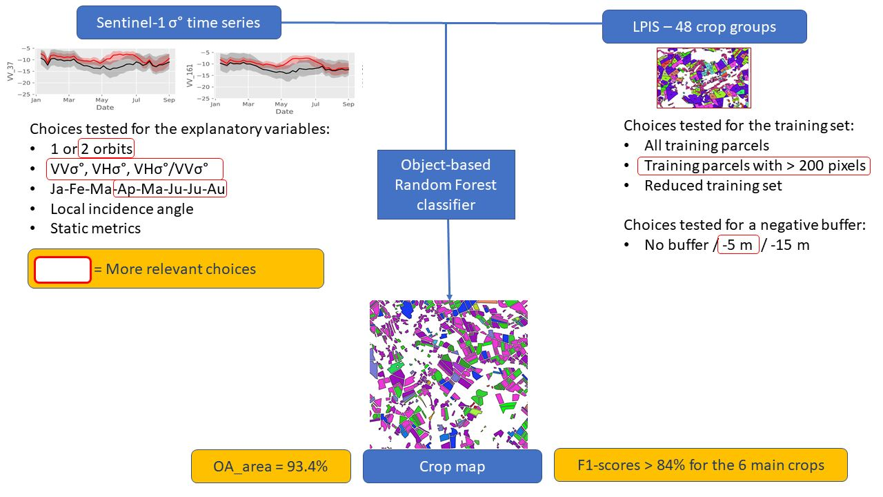
Parameter 1: the SAR input dataset
The explanatory variables used to build the classification model are computed from data coming either from the orbit 37 only, or from the orbit 161 only, or from both orbits 37 and 161. This impacts the number of images used during a considered period and the acquisition time of the images.
Comparing the results obtained from both orbits and from a single one allows to know if a higher temporal resolution (by doubling the number of acquisitions for a considered period) improves the quality of the crop type identification.
Images are acquired at different times depending on the orbit: early in the morning or late in the afternoon. The interest of testing each orbit separately is also to assess whether the acquisition time is important. For instance, images acquired early in the morning could be affected by dew.
Parameter 2: the explanatory variables
The starting idea is that the different crop types can be distinguished using temporal profiles of spectral features extracted from the SAR signal, these features are the explanatory variables of the model to be calibrated. Object-based features are preferred over pixel-based features because of the speckle effect, which needs to be filtered out or averaged out by working at object level. In the context of this study, this is possible since the parcel boundaries are known, and this is also true in each member states in the context of the CAP.
In this study, we have used the per-field mean backscattering coefficient (σ0), which is extracted for each parcel and each available date. The mean is computed as the average over the pixels whose center falls inside the parcel polygons after internal buffer application. Notice that all computations are done in linear units. This is done for both VV and VH polarizations. For each parcel, this gives two time series per orbit, which are used in all scenarios.
In addition to VV and VH, the effect of adding a third time series per orbit, called VRAT, is considered. It is defined as the ratio VH/VV. Indeed, in [40], the authors recommend using VH/VV to separate maize, soybean, and sunflower, which could be applied to other crop types. This quantity is also considered as a variable sensitive to crop growth in several other studies [41,42,43] and thus seems to be possibly a variable of interest for our purpose of crops classification.
Finally, the effect of adding some static variables is studied. For each orbit, the per-field mean of the local incidence angle is computed, together with its standard deviation. This is motivated by the fact that all types of cultural practices—that differ depending on the crop type—cannot be carried on in steep parcels and inhomogeneous reliefs. Hence, the local incidence angle and its intra-field variation could be correlated to the crop type cultivated in a parcel. Since the incidence angle is an almost constant value in time, we take it at a unique date only, which is on 3 May 2020 for orbit 37 and on 29 April 2020 for orbit 161. Some temporal statistics are also added: the mean, the minimum, the maximum, the range, the standard deviation, and the variance are computed for each of the VV, VH, and VRAT time series. For each orbit, there are thus 6 static variables for each time series and 2 for the local incidence angle.
The results obtained with and without these additional variables are compared in order to assess whether they are worth the additional model complexity and data preparation.
Parameter 3: the buffer size
The noise in the time series caused by heterogeneous pixels on the borders of parcels might be reduced by introducing an internal buffer before computing the per-field mean of the backscattering coefficient, thus keeping only clean pixels to represent the parcel. In some cases, it might also mitigate the negative effect of the imperfect geometric accuracy of the image. As was suggested in [44] in the context of a Sentinel-2 analysis, a buffer size of −5 m is chosen in the present study. Another possible source of noise is the fact that the edges of the fields are sometimes managed differently from the central part of the fields (different machines passage orientation or inputs interdiction for example), which causes heterogeneity in the parcel signal. From that point of view, a bigger buffer size of −15 m might ensure a higher probability of having homogeneous pixels for a given parcel. However, a bigger buffer size implies that less pixels are used to average the parcel signal, which is less efficient to filter out the speckle. Therefore, the three following buffer sizes are tested in this study: 0 m (no buffer), −5 m and −15 m. In the −5 m scenario, no buffer is used on the parcels whose polygon after the buffer application is either empty or too thin to contain any pixel (1% of the parcels). In the −15 m scenario, for the parcels whose polygon after the −15 m buffer application is either empty or too thin to contain any pixel, the polygon from the −5 m buffer scenario is used (−5 m buffer for 7% of the parcels and no buffer for 1%). Notice that even when no buffer is applied, some parcels are too thin to contain the center of a SAR pixel, which implies that no signal can be extracted (0.007% of the parcels). Moreover, notice that, because of the “cascading” buffer application, the use of a buffer is more computationally demanding. Indeed, the extractions must be done for the buffer for all the parcels, then the extractions must be done for all smaller buffers for subsets of the parcels, since the number of pixels contained in a parcel is only known after the extraction. The percentage of parcels corresponding to each buffer is summarized in Table 2.
Parameter 4: training set
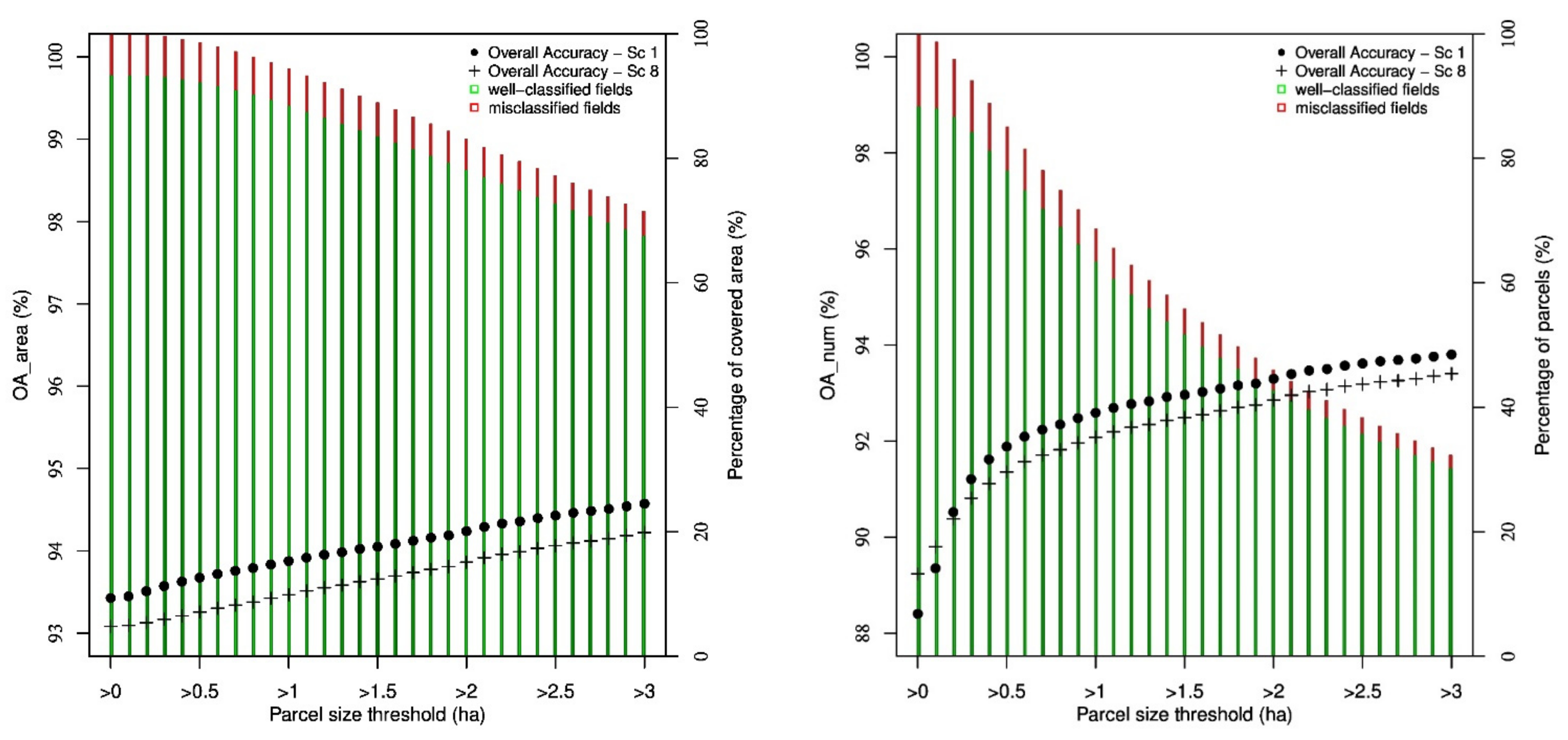
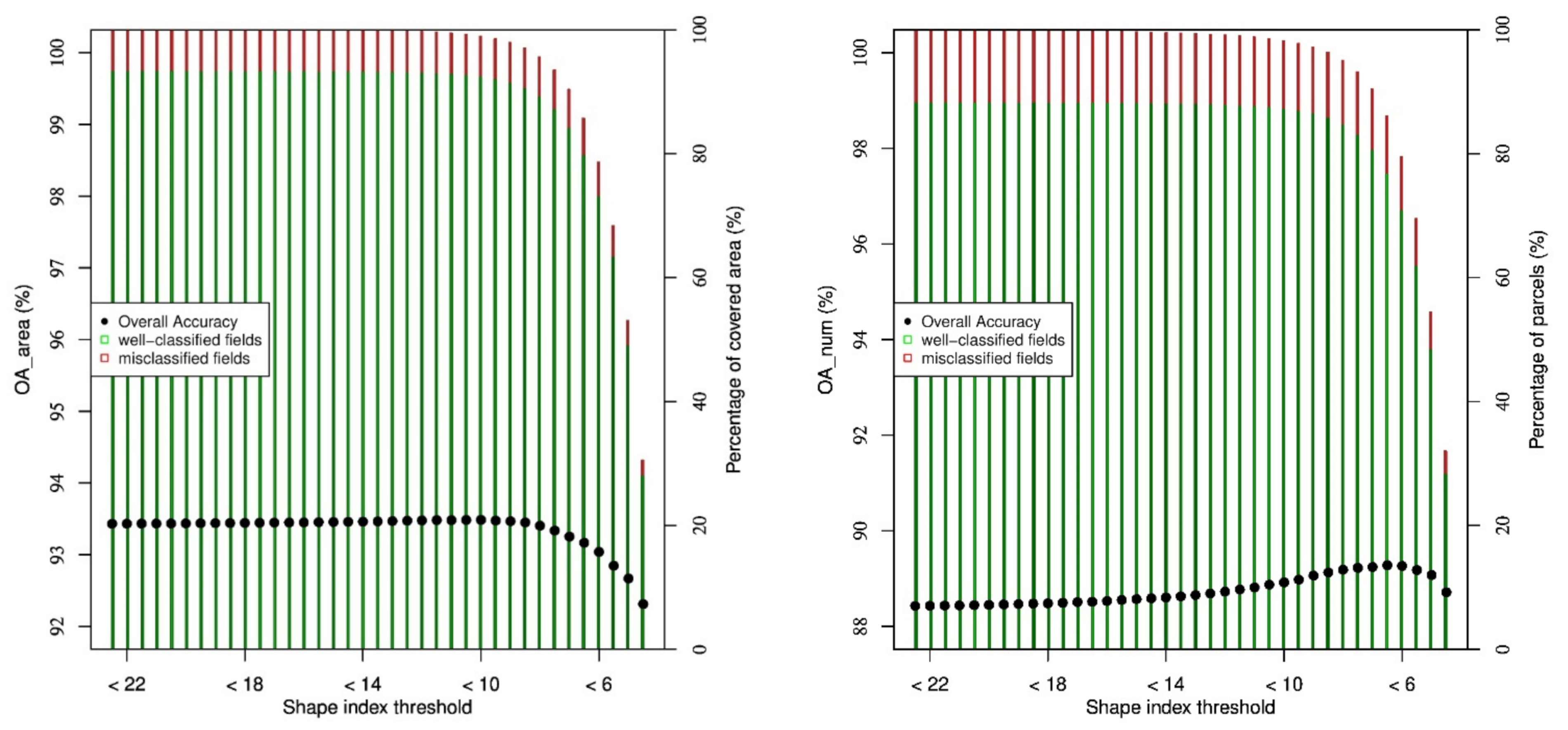
The set of all parcels is split in two disjoint halves, one being used to train the model and the other to score it. In order to improve the model quality, it is trained only on a subset of the training parcels, considered as having a good signal quality. For instance, small parcels are discarded since, because of the statistical uncertainties encountered in the SAR signal due to speckle, [45] recommends averaging the signal over a certain number of pixels. Therefore, a ‘clean’ training dataset is built by selecting only the training parcels which contain at least 200 pixels for all dates after applying the buffer. Notice that in preliminary exploratory studies, some other criteria were considered. For instance, oddly shaped parcels were discarded based on the value of the ratio perimeter over square root of the area. Moreover, the parcel homogeneity was quantified in terms of the per-field standard deviation of the SAR sigma nought. However, these criteria were not retained since they did not seem to lead to significant improvements. The clean dataset contains 64.5% of the parcels in the full training set, and it is used in all the scenarios, unless otherwise specified. To assess the effect of using such a strict screening, a specific scenario is considered that uses the full training dataset to check if the score is then indeed lower.
On another vein, in some situations, only a very small training dataset might be available. In order to investigate the impact on the classification accuracy of a drastically limited training dataset, another scenario is considered where the model is trained using only 10% of the clean dataset. This leads to 3.2% of the full dataset and corresponds to about 6850 parcels. Such a calibration dataset is of the order of magnitude of a large field campaign feasible on the ground.
Parameter 5: the period of SAR acquisitions
This study compares different periods of the year for the time series used by the classification model. First, four periods are defined as starting in January and having different lengths: until May (5 months), June (6 months), July (7 months), or August (8 months). In this case, a shorter period would have the operational advantage of providing classification results earlier in the year, before the harvest time. In addition, 7 periods are defined as ending in August and beginning on different months: from February (7 months) to August (1 month). In this case, the operational advantage of a shorter period would be to deal with a smaller amount of data, which eases the procedure.
Scenarios
Table 3 gives a summary of all the scenarios that are considered, listing the corresponding choices made for each parameter.
In the training set column, “full” means that the full calibration set is used, without any quality filtering, and “10% clean” means that only 10% of the clean parcels are used. The number of acquisition dates for each orbit is also given. Nfeatures is the resulting number of features (i.e., explanatory variables) attached to each parcel that will feed the classification model. For instance, in the reference scenario, for each orbit (37 and 161), there are 2 features for the local incidence angle, plus, for each time series (VV, VH, and VRAT), 40 SAR images and 6 temporal statistics (mean, min, max, std, var, and range). This gives a total of 2*(2 + 3*(40 + 6)) = 280 features. The last two columns give the relative size of the calibration and validation sets compared to the total number (211,875) of considered parcels in the study area.

2.3.3. Classification Model

For our purpose, supervised machine learning is a natural choice since a lot of reference data are available from the farmers’ declaration. Dealing with a large input dataset and a big number of features (but not big enough to require neural networks), a random forest (RF) classifier is chosen as the classification model. Moreover, previous experience carried out in the benchmarking of Support Vector Machine (SVM), decision trees, gradient boosted trees, and RF models in the context of crop classification [20] showed that RF performs generally better, even if SVM is expected to provide better classification results in the specific case of classes with few calibration samples.
The RF is implemented and trained using the python scikit-learn package. Because the goal of this study is not to optimize the machine learning model itself, the default hyper-parameters are kept. Exception is made on the number of trees, which is fixed to 250 in order to reduce the training time without significant performance drop.
Cross-validation is used to assess the model’s performance (full details are given in Section 2.3.4). As previously mentioned, the set of considered parcels consists in those agricultural fields of the LPIS that are located under both orbits 37 and 161. When training a RF model, this set is randomly split in two disjoint equally sized subsets, a validation dataset and a training dataset. The splitting is stratified, that is, each crop group is equally represented in both datasets.
The training dataset is used to calibrate the RF model and is totally independent of the validation dataset.
The validation dataset is used to compute two overall performance scores for the RF: OAnum, the overall accuracy based on the number of parcels (percentage of well-classified parcels compared to the total number of parcels), and OAarea, the overall accuracy based on the area (percentage of well-classified hectares).
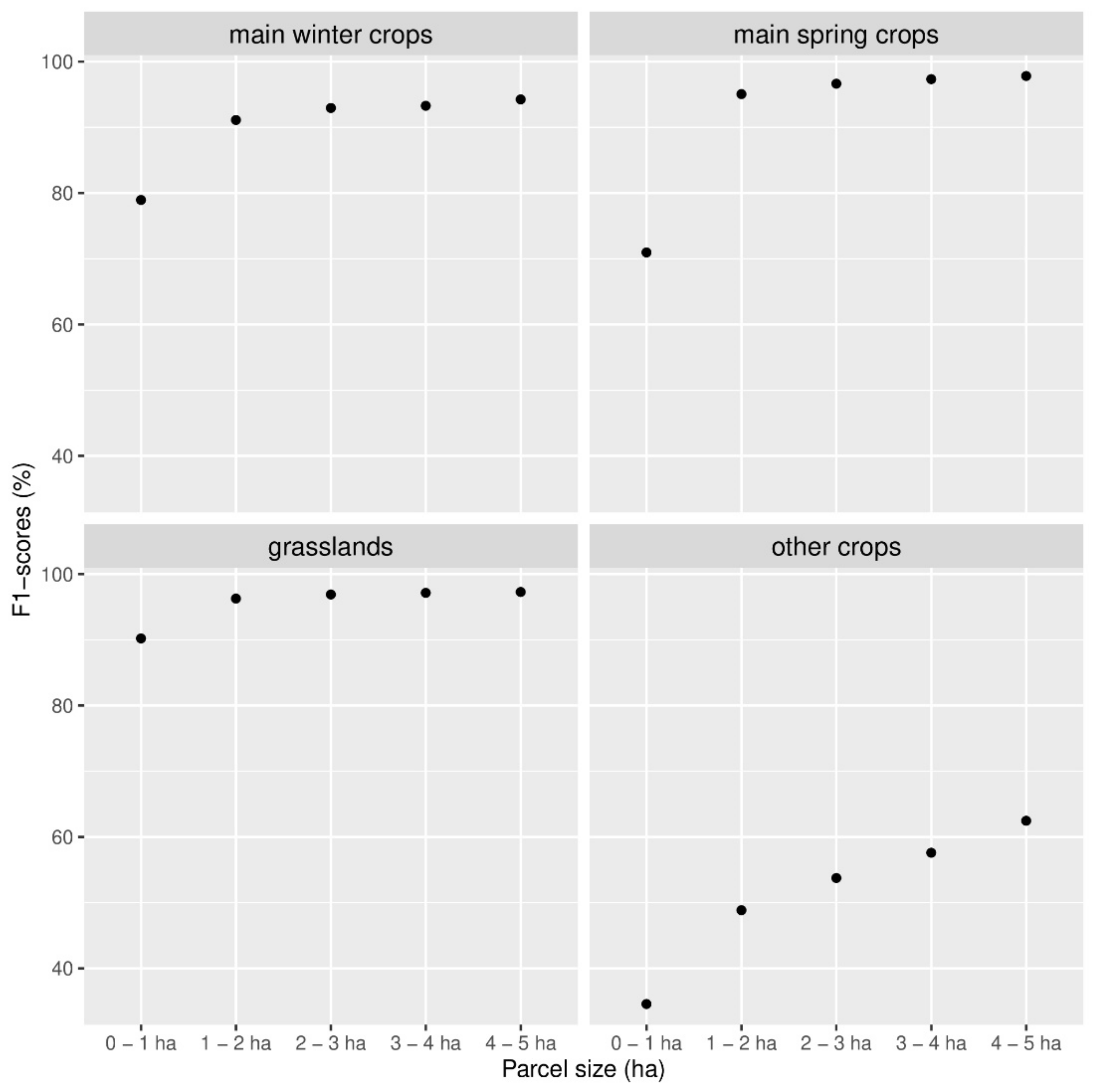
In addition, the F1-score of each crop group is used. In this multi-class classification context, it is defined as the harmonic mean of the group precision and recall (whose definitions are standard):
F 1 g r o u p = g = 2 P r e c i s i o n g r o u p = g     R e c a l l g r o u p = g P r e c i s i o n g r o u p = g   +   R e c a l l g r o u p = g .
For each classified parcel, a confidence level is also assigned to the predicted class. It corresponds to the percentage of trees in the RF that predict the given class.
Notice that the few parcels for which no signal can be extracted because they are too small (see Table 2) are considered as misclassified in the validation set. However, this has a negligeable effect on the scores since they represent 0.007% of the parcels (0.0001% in terms of area).

2.3.4. Test of Statistical Significance

There are several sources of randomness in the building of the RF classification model corresponding to each scenario: the training/validation split and several random choices in the RF initialization and training. This leads to some randomness in their performance scores, and therefore, the best scenario for a given training/validation split might not be the same for another split. This is especially true given that, as will be seen in the next section, the scores are sometimes very close. A test of statistical significance is therefore conducted in order to assess whether the difference in score for two scenarios is significant or if it might just be due to a random fluctuation.
The idea is to define several pairs of training/validation datasets and, for each scenario, to build several RFs, one for each pair. This gives an insight on how strongly the score of each scenario fluctuates. However, naively estimating the variance by computing the standard deviation of the scores is not recommended because the latter are strongly correlated (typically, the training datasets of each pair overlap and are thus not independent (same for the validation datasets)). Using a very high number of pairs would lead to an underestimated variance. This is therefore a complex question, to which many answers are proposed in the literature, some of them being summarized and compared in [46]. Given the situation encountered in this paper, the 5 × 2 cross-validation F-test introduced in [47] is chosen—which is a slight modification of the popular 5 × 2 cross-validation t-test originally defined in [48]. Here is a quick overview of the procedure. As previously mentioned, the goal is to repeat the training/validation several times for each scenario to estimate the score fluctuations, while finding a right balance between having a high number of repetitions, lowering the overlapping between all the training datasets (same for the validation datasets), and keeping enough data in each set. First, the full dataset is randomly split in two equally sized stratified parts, and this is independently repeated 5 times. This leads to 5 pairs of 50–50% disjoint subsets of the full dataset. Then, for each scenario and each pair, two classification models are built: the first one using one part as the training set and the other part as the validation set, and the second one by switching the role of each subset. For each scenario, this gives thus 10 performance scores. When comparing two scenarios, a standard hypothesis test is conducted, taking as null hypothesis that they both lead to the same score. From the 20 scores, a number t is computed—its exact definition can be found in [47]—and the author argues that its statistic approximately follows a F-distribution, allowing to compute the corresponding p-value. If this p-value is higher than a chosen threshold α, the null hypothesis that the scenario scores are equal can be rejected at the corresponding confidence level. Now, the fact that several scenarios are compared has to be taken into account in order to get the expected p-value for the multiple comparisons altogether. The Bonferroni correction is chosen, which suggests using α divided by the total number of comparisons as the p-value threshold of each individual comparison. In this study, α is fixed to 0.05.
Since the goal of this study is to evaluate the effect on the classification performance of each parameter separately, there is no need to compare all the scenarios together. Instead, in order to reduce the number of comparisons, a reference scenario is chosen, against which all the other ones are compared. It corresponds to the scenario with both orbits 37 and 161 considered, all the explanatory variables (VV, VH, and VRAT time series + static variables), the 8 months period, a −5 m buffer, and the clean training set.
As a final note, it should be reminded that all these statistical tests are based on approximate hypotheses and that the numbers should therefore not be blindly taken as an absolute truth.

3. Results

This section first includes a general overview of the results in terms of the overall accuracies. A deeper analysis is then given in terms of the F1-scores of each crop groups. Finally, the classification performance is analyzed considering the scenario’s parameters described in the previous section.

3.1. General Results of the Classifications Using SAR Data

Table 4 summarizes the performance scores for each scenario. For each of them, the values of the parameters described in the previous section are given. The scenario 1 is the reference scenario mentioned earlier. The overall accuracies (OA) correspond to the mean of the OAs of each of the 10 models and are supplemented by their standard deviation. Two kinds of Overall Accuracies are computed: the OAarea which is equal to the percentage of well classified area and the OAnum which is equal to the percentage of the number of well classified fields. This gives two different points of view when comparing the scenarios. In the following, OAarea is generally used, unless when OAnum is more relevant.
A first key finding of this study shows that for most scenarios, the scores are very close, which is the motivation to investigate whether the score differences are statistically significant. In the tables, the p-value corresponds to the aforementioned hypothesis testing that the scenario score (OAarea) is different than the reference one. The significance column indicates whether that p-value is lower than the chosen Bonferroni corrected threshold, i.e., 0.05/18 (18 being the number of comparisons made).
OAarea is always higher than 90% except for the two worst scenarios. For the reference scenario, OAarea reaches 93.43% (both orbits are used, the longest period is considered, all the explanatory variables are included, the clean training set is used, and an internal buffer of −5 m is applied). This is the best score, together with the other six top scores as they are not statistically different from the reference’s one. These scores correspond to the scenarios 5 (−15 m buffer and all variables) and 6 (−5 m buffer and all variables excepted static variables) and to the four scenarios whose period begins in February, March, April, and May.
This method reaches high performance compared to other studies. Indeed, in the optical domain, in [49], the authors reach an overall accuracy of 83% using a random forest classifier for 14 classes from Landsat surface reflectance in Yolo County, California. In [3], the authors discriminated the 5 main crops in three entire countries with overall accuracies higher than 80% using Sentinel-2 and Landsat time series. In the SAR domain, in [32], the authors classified 14 crop types (including grasslands) in Denmark (over 254 thousand hectares) from SAR Sentinel-1 data time series with an average pixel-base accuracy of 86%. In [22], the authors predicted 8 crop types with a maximum accuracy of 82% (OAnum) with a pixel-based random forest classifier and Sentinel-1 and Sentinel-2 dataset over Belgium’s agricultural land that covers more than 1,300,000 hectares. In [39], the authors reach an overall accuracy of 94.6% using 2-d CNNs model for classifying land cover into 11 classes including 8 agricultural classes in Ukraine from LandSAT and Sentinel-1A images. However, regarding their high score, it must be noticed that this study discriminates less classes of crop types and does not focus only on agricultural classes. It includes the classes “water” and “forest”, whose User and Producer Accuracies are very high (near 100). This pushes the overall accuracy higher than if only agricultural crop types were considered.
A first look at the numbers indicates that the four parameters that give some noticeable performance differences are the orbit, the period, the presence of the VRAT in the explanatory variables, and the training sample. Further comments will be made later in the “Impact of the scenarios’ parameters” subsection.

3.2. F1-Scores of the Crop Groups

Table 5 shows the F1-scores (in terms of the number of parcels, not the area) for each crop group, sorted by their prevalence. The prevalence is both given as the percentage of the number of parcels of the group in the validation dataset (Num) and as the percentage of the area covered by the parcels of the group (Area). Recall that, for each scenario, 10 classification models are computed, corresponding to different pairs of training/validation datasets. The prevalence is (almost) the same for all of them, but the F1-score does vary. The F1-score given in the table is the mean of the F1-scores corresponding to each model. Some crop groups, although present in the validation dataset, are never predicted by some models, and their F1-scores are then set to ‘NaN’. The column ‘no grasslands’ will be described later.
In the reference scenario, the 6 most represented crop groups have an F1-score higher than 84%. It is actually higher than 90%, except for “Maize”. In that case, its recall is high, but its F1-score is lowered by its low precision. This is because a large proportion of mis-classified parcels are classified as Maize (this is also the case for the grasslands, but it does not impact their precision as much because of their higher prevalence). Nine crop groups get F1-scores higher than 84%, and they represent 89.5% of the parcels (91.6% of the area).
Table 5 shows that “sugar beet” has the highest F1-score, which is equal to 95.52%. Moreover, F1-scores tend to be higher for the most represented crop groups, always higher than or equal to 83.97% for the six most represented groups. For the groups with lower prevalence, there is no clear relation between the prevalence and the F1-score. It is interesting to notice that three crop groups with a low prevalence get a high F1-score: winter rape, spring pea, and chicory. Figure 2 shows the temporal evolution of the mean of the backscattering coefficient over all winter rape parcels (in red), in comparison with the same profile evolution for all the other agricultural parcels (in grey). This figure highlights a specific behavior of VH for the winter rape during the end of the spring. The winter rape is indeed different from the other winter crops at this period. The end of the spring corresponds to the end of the flowering, the steam elongation and branching, and the pod and seed (fruit) development and ripening of winter rape. The specific geometry of the winter rape with a high stem and a lot of branches at this period certainly explains the higher VH signal since this crop exhibits more non vertical elements compared to the other winter crops.
Now let us look at some low F1-scores. The first three groups which get a low or no F1-score are “Alfalfa”, “Fallows”, and “Others”. These groups are often classified as grasslands: 86%, 64%, and 55% of the parcels for “Alfalfa”, “Fallows”, and “Others”, respectively. This can be explained by the fact that, although these groups are considered as distinct in the farmers’ declarations, the reality on the field is very similar between these three groups. First, the group “Others” includes fodder crops (56% of the parcels of the group) that can be grasslands. Secondly, an alfalfa grassland can be claimed by the farmer either as alfalfa or as temporary grassland. Thirdly, the “Fallows” group includes herbaceous fallows that, on the field, are crop cover similar to grasslands, even if their management differs.
Regarding the bad score of the group “Others”, it should also be noticed that it includes 13 different crop types, sometimes very dissimilar such as greenhouse vegetables, oleaginous or proteaginous crops. Therefore, that group does not really makes sense from an EO point of view. In light of the previous remark on grasslands, it is therefore interesting to notice that this bad score is in fact due to a strength of the classification model: its ability to recognize grasslands within a group of parcels of heterogeneous crop types.
Nevertheless, this illustrates a weakness of using the LPIS as a training set for crop classification. Indeed, the declaration of the farmers can be ambiguous for some crop types, which can confuse the random forest classifier.
Analysis excluding the grasslands
Since the high overall accuracies are driven by the large proportion of grasslands (more than half of the number of parcels), which get a high F1-score, the classification is also done for arable land only, excluding the grasslands. This represents 93,832 parcels, from which 50% are kept as a validation dataset, and 36% are used in the calibration dataset (half of the agricultural parcels excluding grasslands that contains more than 200 pixels after applying the buffer). The other parameters are the same than those used in the reference scenario 1. As for the other scenarios, 10 classification models are computed, corresponding to different random splits of training/validation datasets. OAarea, the percentage of well-classified area, equals 90.44%, which is 3% lower than for our reference scenario 1. Nevertheless, these results give globally better F1-scores for the arable land than the results obtained when the grasslands are included (see Table 5—right column), especially for the groups “alfalfa” and “other” (the latter being the 6th most prevalent crop group). Indeed, as was mentioned earlier, the parcels in these two groups are often grassland in reality, and when grasslands are included in the training sample, these parcels are often classed as grasslands, which is not a real error but an error due to the claim system that permits to a farmer to claim an alfalfa parcel as grassland or alfalfa. The F1-score of “permanent crop” also increases. In scenario 1, 50% of such parcels are classified as grasslands, which can be explained by the fact that fruit tree crops mainly represent this group (92% of the parcels). Hence, they can be mixed up with wooded grasslands. For the other crop groups, which are groups more different from the grasslands on the ground, the F1-score does not change drastically.

3.3. Impact of the Scenarios’ Parameters

In this section, the classification results are further analyzed considering the variation of the five parameters described in the “Methodology” section: the SAR orbit, the explanatory variables set, the period of the time series used for signal extraction, the use of different internal buffers on parcel polygons before SAR signal extraction, and the quality and size of the training sample.

3.3.1. Impact of the SAR Orbit on the Classification Performance

The effect of using different SAR orbits to compute the explanatory variables is described hereafter.
The considered orbits are orbit 161 and orbit 37. They differ by their hours of acquisition—which are around 5:30 p.m. and 6:00 a.m. (UTC)—and their orbit orientation: ascending and descending tracks respectively. The time of acquisition has a global impact on the signal because of the presence of dew during the morning that can enhance the signal [50]. The orbit track orientation also has an impact on the signal at the parcel level since the local incidence angle is different and the relative azimuth angle between the SAR beam and the plant rows differs as well (considering the crops cultivated in rows such as maize, potato and sugar beet).
The results first compare the classification performance corresponding to three different SAR datasets:
-
SAR data acquired on both orbits 37 and 161 (reference scenario 1),
-
SAR data acquired on orbit 37 (scenario 2),
-
SAR data acquired on orbit 161 (scenario 3).
The results show that the higher number of explanatory variables given by combining the two orbits leads to a better overall accuracy (both in terms of area and of number of parcels), but the computing cost is doubled. When using only a single orbit, the score drops by less than 1%. This is a small difference, but the significance test shows that it is not due to random fluctuations. In the specific case of determining the crop type in the context of the CAP, the best accuracy is needed in order to reduce the number of fields visits. Indeed, for 100,000 parcels to monitor by a Member State, a drop of 1% of OAnum leads to 1000 additional misclassified parcels, increasing the required number of fields visits. However, a lower score might be perfectly adequate for other applications such as regional scale agricultural statistics or yield prediction for the main crops, where reducing the computational cost might be more important.

3.3.2. Impact of the Set of Explanatory Variables on the Classification Performance

In all the scenarios, the VV and VH polarizations are used as explanatory variables. The effect of using three additional kinds of explanatory variables is here analyzed: the ratio VH/VV, local incidence angle per-field statistics, and temporal statistics.
In addition to the time series corresponding to the VV and VH polarizations, a third one corresponding to the ratio VH/VV, called VRAT, is added to the explanatory variables. In scenario 7, the ratio VH/VV (called VRAT) is excluded. This decreases the OAarea, by 0.46%, and the significance test shows that the difference is significative from a statistical point of view. Regarding OAnum, the performance drops by 1%. This shows that VRAT contains some useful information that the RF cannot extract solely from the values of VV and VH. However, depending on the application, the additional model complexity and computer processing time might not be worth the performance improvement.
The influence of including some static variables has also been studied. These static variables include, for each orbit, the per-field mean of the local incidence angle, together with its standard deviation. They also include some temporal statistics: the mean, the minimum, the maximum, the range, the standard deviation, and the variance are computed for each of the VV, VH, and VRAT time series and each orbit. This gives 2+36 additional variables per orbit. In order to assess whether these variables are useful, scenario 8 tests the performances of the classification without including them to the explanatory variables. The results show that removing them does not change the classification performance. Looking at the OAnum, one can even see that it even gets better for that scenario.

3.3.3. Impact of the Buffer Size on the Classification Performance

As was explained earlier, applying an internal buffer to the parcel polygons before averaging the pixel values of the SAR signal might help reducing the signal noise. This section compares the use of three different buffer sizes (scenarios 1, 4, and 5): no buffer, −5 m, and −15 m.
Besides removing mixed pixels along the parcel borders, using a higher buffer size might remove noise introduced by different agricultural practices at the edges of the parcel. On the other hand, the application of a higher buffer size reduces the number of pixels considered to compute the per field mean, which might be in contradiction to the necessity of averaging over many pixels to increase the signal consistency regarding the speckle present in the SAR signal. Since the results show no difference between applying a buffer of −5 or −15 m, these two effects seem to either be negligible or to counterbalance themselves. A high buffer should be preferred in some specific cases: poor geometric quality of the polygons or misalignment of images.
Regarding the effect of applying a buffer at all, the results show a statistically significant difference between applying a −5 m buffer and using no buffer. However, because the improvement due to the buffer is very small (0.27% in terms of area), the added complexity might not be worth it, depending on the application.

3.3.4. Impact of the Quality and Size of the Training Sample on the Classification Performance

One of the keys to building a good model is to have a good and big enough ground truth dataset for the training sample.
Comparison of the scenarios 1 and 8 focuses on the quality of the training dataset. Recall that it has been chosen to train the model using a ‘clean’ dataset, which contains only parcels containing at least 200 pixels, since they are considered to have a cleaner signal. Such parcels represent 64% of the parcels; thus, the training dataset contains 32% of the whole number of parcels. In order to assess whether such selection is useful, in scenario 8, no filtering is done, and the calibration dataset counts thus 50% of the whole number of parcels. The results show that the cleaning of the training set leads to slightly better results, increasing the OAarea by 0.35%. As this cleaning is easy to perform and also allows to reduce the processing time, it is thus advisable to apply it to the calibration dataset before training the model. However, it must be noticed that when considering OAnum, using the full calibration dataset leads to a better score. This is more deeply discussed in the “Discussion” section of this paper.
In another vein, to assess the impact of the size of the training dataset, scenario 9 uses a smaller training dataset. From the clean dataset used in scenario 1, only 10% of the parcels are used to train the model, which is about 6850 parcels, i.e., 3.2% of the whole number of parcels. When reducing the training sample size in such a drastic way, the OAarea drops by 1.78% only, from 93.43% to 91.65%.
The high OAarea obtained in each case presents very promising results for regions where poor ground data are available and field surveys are required. Moreover, considering that the declaration of the farmers can be ambiguous for certain crop types (for instance, the confusion between fodder, grasslands, and alfalfa which was mentioned earlier) or erroneous; a field visit of 6850 parcels could, at the Walloon Region scale, be considered to improve the training dataset quality.

3.3.5. Impact of the Period of the SAR Time Series on the Classification Performance

One of the significant changes to be considered for the next CAP reform is to provide Near Real Time information to the farmers all along the year concerning their agricultural practices and changes observed by remote sensing images. To assess this issue, the evolution of crop identification quality over time is also analyzed by comparing scenarios 1, 10, 11, and 12. From the results of Table 6, one can see that the overall accuracies increase with the length of the period of the SAR time series, both in terms of area and number of parcels. To have a better insight of the impact of the period length on each crop group, Table 6 gives the F1-scores of each crop group for the 4 different periods. The F1-score of grasslands reaches more than 93.7% for all considered periods. Regarding the two most represented winter crops, which are harvested in July, they are classified with a F1-score of at least 0.86% already since the end of May, but the F1-scores increase by at least 3% if the considered period includes the whole winter crops season up to the harvest. Regarding the main spring crops, the F1-scores increase strongly between the first two considered periods and then increase more slightly. The spring crops are harvested in September or October. The present analysis shows that 5 of the 6 most represented crop groups can be recognized before their harvesting dates with a F1-score higher than 89%. The maize does not reach such high score and its F1-score equals 84% about 2 months before its harvest. As explained before, the lower F1-score of maize is due to the fact that a large proportion of the mis-classified parcels are classified as maize, which lowers its precision score. As before, some crop groups are never predicted by some models, in which case their F1-scores are set to ‘NaN’.
Since three of the most represented crop groups (maize, potato, and sugar beet) are spring crops which are sown from March to May, the classification has also been tested for periods beginning later in the season. Indeed, the information derived from time series before their sowing date can bring noise for these crops as different field practices are encountered on these parcels before the sowing (presence of different types of catch crops or absence of catch crop for instance). Considering OAarea, the results in Table 7 do not show any significant score differences whether the classification starts in May or before. However, it should be noticed that from the point of view of OAnum, there appears to be a noticeable decrease in the performance. A higher decrease of the score is met if the three first months including March are excluded from the time series.
As before, the F1-scores of each crop group for the different periods are listed in Table 7. This gives a deeper insight on the performances in terms of the percentage of parcels. It also allows to see whether beginning later in the season might be beneficial for some crops by removing some noise coming from irrelevant months.
The best F1-scores for each crop group are highlighted in bold black in Table 7. One could have expected that the period giving the best results for a given crop would depend on when the crop is in place. For grasslands and winter crops (the latter being mainly sewed in Autumn and harvested in July), this would correspond to the longest period, from January to August. For crops starting later in the season (like maize, potato and sugar beet which are sewed mainly in April and harvested in Autumn), one could think that the first months of the year would be irrelevant. However, the present results show that reality is more complex. Among the most represented crops that are in place during the beginning of the season, only grasslands and winter wheat get a higher score if the whole period is used. For the 2nd and 3rd most represented winter crops (winter barley and spelt), the best F1-scores are reached when the considered SAR time series begins in April. Regarding the spring crops, the conclusions are also diverse. Contrary to the previous hypothesis, maize gets a significantly better score when starting in January rather than in April or May. The January score is also better for sugar beet, although the scores are similar up to April (but lower starting from May). For potato, the best score is reached when starting in May, although longest periods show similar results.
Thus, the considered period may be adapted to the user’s goal. Depending on whether the aim is to obtain an early map of the crop types, or to more accurately recognize crops appearing later in the season, a different ending month for the time series can be chosen. For some specific crops, using a times series starting later in the season can be beneficial. Subsequent classifications could thus be performed to first discriminate some crops and then the other ones.

4. Discussion

This section first addresses a major constraint linked to the use of SAR images: the presence of rain or snow that affects the SAR signal. The robustness of the classification regarding that aspect is discussed in Section 4.1.
Secondly, the discussion analyses how the classification accuracy depends on some characteristics of the parcels: their classification confidence level, their size, and their shape. The objective is two-fold. First, this allows to understand whether the classification is relevant on the whole range of that characteristic (for instance, is the classification accurate for oddly shaped parcels?). Furthermore, considering a threshold on those characteristics allows to identify a subset of the parcels for which the global classification accuracy is higher.

4.1. Impact of Rain and Snow on the SAR Signal

The SAR signal is not affected by the presence of clouds, but it is sensitive to rain and to the water drops on the vegetation. The presence of rain or water drops during the time acquisition of the SAR data used in the present study can be assessed thanks to ground truth meteorological data. The PAMESEB meteorological stations provide in situ precipitation measures recorded on an hourly basis at 30 locations in the WR (Source: CRA-W/Pameseb network—www.agromet.be—2 February 2021).
On the 80 selected SAR Sentinel-1 acquisitions on tracks 37 and 161 between 10 January 2020 and 02 September 2020, 52 images were acquired less than 2 h after or during a rainfall in at least one of the PAMESEB stations located in our study area. The average number of images from all Pameseb stations acquired just before or during a rainfall at the station is five. Thus, on average, the number of rain-free SAR images at a station is 75.
Comparatively, out of the 95 optical Sentinel-2 acquisitions over the T31UFR tile during the same period of eight months, only 24 acquisitions are useable (i.e., cloud-free) on average at the agricultural parcel level.
Moreover, the presence of snow also affects the SAR signal. On the 80 SAR Sentinel-1 acquisitions on tracks 37 and 161, 11 images were acquired when the presence of snow was recorded by the Royal Meteorological Institute of Belgium.
Despite the inclusion in the dataset of these images acquired when rain and snow occurred, the combination of the high number of acquisitions and the automatic selection of the most meaningful explanatory variables by the random forest seems to overcome the problem.

4.2. Evolution of the Classification Performance in Terms of the Classification Confidence Level

To the class assigned to a parcel by the classification model is linked a confidence level of belonging to this class (percentage of the trees in the forest that predict the given class). Figure 3 shows the evolution of the overall accuracy in function of a threshold on the confidence level. For each value of the threshold, the corresponding OA is computed only on the parcels of the validation dataset which are classified with a confidence level higher than the given threshold. Recall that 10 models are trained for each scenario: the represented OA is, as before, the mean of the 10 corresponding overall accuracies. On the left graph, the OA is computed in terms of the area (OAarea), while on the right, in terms of the number of parcels (OAnum). The OA (black dots on the graph) increases with the confidence level threshold. However, this must be balanced by the fact that less parcels are classified since the number of parcels meeting the threshold criterion decreases. This is shown by the bars on the graph, which represent the proportion of parcels in the validation dataset which satisfy the confidence level threshold. For OAarea, this proportion is given as the percentage of the area covered by these parcels, and for OAnum, as the percentage of the number of parcels. These bars also represent the proportion of well- and mis-classified parcels (green and red bars, respectively).
Considering a threshold on the confidence level allows to identify a subset of parcels on which the global accuracy is higher. For instance, considering only the subset of parcels classified with a confidence level higher than 92%, OAarea reaches 99.03%. However, the downside is that this subset covers only 64.7% of the total area of the validation dataset. This kind of analysis allows to choose the best compromise between the accuracy of the classification and the area covered by the classification. In this case, a good compromise is a threshold of 32% on the confidence level: it leads to an OAarea of 95% while still covering 97% of the area. In the case of OAnum, the decrease in the number of parcels is faster. If one is more concerned about keeping a high number of parcels instead of a high covered area, a threshold of 24% is therefore preferable: 95.7% of the parcels are classified and OAnum is 90.9%. Figure 3 also shows that the confidence level is linked to the size of the parcel as one can see that the parcels having a confidence level higher than 96% covers more than half of the area of the WR while it concerns only about 33% of the number of parcels.
In the framework of the CAP, a progressive classification process could be imagined over time. The classification could be done several times during the growing season and a parcel would be considered as “well-classified” as soon as its confidence level reaches a chosen threshold.

4.3. Evolution of the Classification Performance in Terms of the Parcels Size

In Table 4, the percentage of well classified area is always higher than the percentage of well-classified number of fields. This can be explained by a worse capacity of the classification model to classify small fields. Indeed, because of the statistical uncertainties in the SAR signal, the SAR speckle has a strong effect on the signal when considering a single pixel or an average over a small number of pixels. In order to analyze this constraint, Figure 4 shows the evolution of the overall accuracy when considering a threshold on the parcel size. For each value of the threshold, the corresponding overall accuracy is computed only on the parcels of the validation dataset whose area is higher than the threshold. This evolution of the OA is given for the reference scenario (black points) and the scenario 8 which includes all the parcels in the training dataset (black crosses). The bars on the graphs show, for the reference scenario, the proportion of the parcels in the validation dataset (in terms of the area on the left graph and of the number of parcels on the right graph) that satisfy the size threshold. The green and red bars represent the proportion of well- and mis-classified parcels, respectively.
The overall accuracy increases with the parcel size threshold, but at the same time, the number of fields for which a class is obtained decreases. When all the parcels in the validation dataset are included (as in Table 4), OAnum reaches 88.4%. At the other extreme, OAnum reaches 93.8% if only the parcels in the validation sample that are bigger than three hectares are considered, which represents 32.3% of the parcels. The steepest increase of OAnum happens in the range from 0 to 0.5 hectares. Over 1 ha, the increase is not yet significant. This clearly illustrates the difficulty of working at pixel level or with pixels averaging for a small number of pixels with SAR data due to the speckle.
Recall that in the reference scenario, only the ‘clean’ parcels (i.e., covering a minimum number of pixels) are included in the training dataset. Scenario 8 includes all the parcels in the training dataset, and it could be supposed that such scenario would be better at classifying small parcels (since the model is also trained with similar parcel sizes). To quantify this, the black crosses on Figure 4 show the evolution of OAnum for that scenario. One can see that, for small thresholds, the percentage of well classified parcels is indeed higher for scenario 8. However, for a threshold of 0.2 hectare or higher, scenario 1 is better. Notice that the same comparison can be made in terms of OAarea, and in that case, scenario 1 is always better.
Figure 5 shows the value of the F1-score of four different crop categories for five areas ranges. The crop categories are: the main spring crops (maize, potato, and sugar beet, representing 17.3% of the number of parcels and 20% of the area), the main winter crops (winter wheat and winter barley, representing 14.2% of the number of parcels and 21% of the area), the grasslands (55.7% of the parcels, 47% of the area), and the other crops (12.8% of the parcels, 12% of the area). For each of these categories, the F1-score is computed on the subsets of parcels whose size is contained in ranges of one hectare. Notice that we consider ranges here and not a threshold as before. The steepest increase of the F1-score is met for the main spring crops and for the other crops. For the main spring crops, the F1-score is significantly lower for parcels smaller than one hectare, which represent about 24% of the parcels in that category. Except for the other crops, beyond one hectare, the increase of the area has no significant impact on the F1-score anymore.
In landscapes such as Belgian landscape where the agriculture is mainly intensive, the size of the parcel is not an excessively big challenge for working with Sentinel-1 data (the mean of the parcel areas is equal to three hectares). Nevertheless, in other regions, either the use of higher spatial resolution images or the aggregation of adjacent parcels considered as Feature of Interest (i.e., homogeneous areas covered by the same crop, uniformly managed) should be investigated. In [51], the authors demonstrated that the classification performance is much more dependent on the type of cropping systems (including the fields size) than on the classification method.

4.4. Evolution of the Classification Performance in Terms of the Parcels Shape

Other parcels can have very few numbers of pixels inside their polygons, despite having an honorable size: the oddly shaped parcels. For instance, a very long and thin parcel might have a big area but still contain very few pixels. A way to quantify this is to consider the shape index: the ratio between the perimeter of the parcel and the square root of its area. The smaller the shape index, the closer the parcel looks to a nice circle. In the LPIS, the shape index ranges from 3.7 to 57.1, and 99.9% of the parcels (99.98% of the area) have a shape index lower than 20. In order to analyze this constraint, Figure 6 shows the evolution of the overall accuracy in function of a threshold on the shape index. Only the parcels in the validation dataset whose shape index is under the given threshold are considered in the OA computation. On the left, the overall accuracy is computed in terms of the area of the parcels, and on the right, in terms of the number of parcels. As before, the bars represent the proportion of parcels in the validation dataset which meet the threshold criterion (in terms of the area on the left, and on the right, in terms of the number of parcels). The green and red bars correspond to the well- and mis-classified parcels, respectively.
When considering OAarea, the threshold does not lead to any significant score improvement. When considering OAnum, a slight score improvement can be observed, but it must be put in balance with the drop in the number of classified parcels. For instance, a threshold of 8 gives an overall accuracy of 89.2% on the subset of parcels meeting that threshold (instead of 88.4% when all parcels are considered), but this subset only counts 95% of the parcels.

5. Conclusions and Perspectives

In the particular context of the CAP crop monitoring, there is much interest in improving the performances of the crop classification, since it leads to less field visits, i.e., less work for the Paying Agencies.
Moreover, since the availability of optical images is often a problem in region with a frequent cloud cover, such as Belgium, Sentinel-1 SAR images give very promising results to identify the agricultural crop groups. Indeed, this study shows that the combination of the high number of acquisitions and the automatic selection of the most meaningful explanatory variables by the random forest seems to overcome the negative impact of rain and snow on the SAR signal. Using an object-level random forest classifier, 48 crop groups could be classified with an overall accuracy of 93.4% of well-classified area, which is a very nice result compared to the literature. The F1-scores of the six most represented crop groups are always higher than or equal to 84%.
Furthermore, one of the significant changes to be considered for the next CAP reform is the regular information to be provided to the farmers along the season about their agricultural practices. In this respect, the results show that five of the six most represented crop groups can be recognized before their harvesting dates with a F1-score higher than 89%.
Given the several kinds of information that can be extracted for one parcel from Sentinel-1 sensor, one of this study’s aim is to define which are the most relevant explanatory variables that have to be used to improve the classification results quality while not unnecessarily increasing the model’s complexity. The goal is to get the easiest and best performing model. The results show that the addition of the VHσ0/VVσ0 ratio in the explanatory variables and the use of information derived from two orbits (one ascending and one descending) increase the performances. The most relevant period of the time series to consider starts at the beginning of the spring crops growing season until the month after the harvest of the winter crops.
Other choices can improve the classification performances: the use of an internal buffer on the parcel polygons before signal extraction, the selection of the parcels containing more than 200 pixels for the signal extraction in the training sample.
In another vein, this study shows how the classification accuracy depends on some characteristics of the parcels. It is shown that small parcels are still difficult to classify. Indeed, the classification performance is significantly lower for parcels smaller than one hectare. On the other hand, considering a threshold on such a characteristic allows to identify a subset of parcels for which the global accuracy is higher. This kind of analysis helps to choose the best compromise between accuracy and the proportion of parcels that are still taken into account, depending on the user’s need.
This study also addresses the main challenge of have good ground truth data to calibrate a model. Our results show that using a small training dataset (containing 3.2% of the total number of the fields, i.e., about 6850 parcels) leads to an overall accuracy of 91.65% of well-classified area. This is a promising result for regions where poor ground data are available but also in our region since it allows to improve the training dataset with a limited number of field visits.
Here are some perspectives to go beyond the present analysis.
In addition to the per-field mean of the SAR data, the intra-field heterogeneity might be relevant to the classification. The use of time series of, for instance, the intra-field standard deviation, should be investigated.
Moreover, other kinds of explanatory variables computed from the remote sensing data could be used (date of maximum/minimum backscattering coefficient, highest slope of the backscattering coefficient, period during which the backscattering coefficient is higher/lower than a threshold, etc.).
As mentioned earlier, subsequent classifications, using different time periods, could be performed in order to classify the crops one after the others, depending on when they are best recognized. Indeed, in the case of the Walloon crop calendar, a first classification could differentiate grasslands and orchards from other agricultural lands using a period covering autumn and winter since these crops would already be in place during that period. Then, winter crops could be separated from the spring and summer crops using the end of autumn, winter, and beginning of spring periods.
Beyond the improvement of the classification accuracy, the possibility of transferring the model calibration to subsequent crop seasons should be analyzed. On that respect, it should be mentioned that the analyses done in this paper have also been conducted on the 2019 data and that the results and conclusions are similar. However, this is different than using a model calibrated on one season and validated on the next growing season, which might be useful from an operational point of view.

Author Contributions

Conceptualization, P.D., E.B. and C.L.-D.; methodology, A.J. and E.B.; software, A.J. and E.B.; validation, A.J. and E.B.; formal analysis, A.J. and E.B.; investigation, E.B. and A.J.; resources, A.J. and E.B.; data curation, A.J. and E.B.; writing—original draft preparation, initial draft, E.B. and A.J.; review of the writing including results interpretation, A.J., E.B., P.D. and C.L.-D.; writing—review and editing, E.B. and A.J.; visualization, A.J. and E.B.; supervision, E.B.; project administration, E.B. and V.P.; funding acquisition, V.P. All authors have read and agreed to the published version of the manuscript.

Funding

This work was carried out within the framework of the SAGRIWASENT project founded by the Walloon region.

Institutional Review Board Statement

Not applicable.

Data Availability Statement

The SENTINEL data presented in this study are available freely through the COPERNICUS program of ESA. The parcel delineation data are available on request through https://geoportail.wallonie.be/ (13 July 2021). Meteorological data may be requested through https://agromet.be/ (2 February 2021). The exact details about crop groups may be requested from the authors.

Acknowledgments

We would like to thank the agents of the “Direction des Surfaces” of the “Service Public de Wallonie” (SPW) for their collaboration. We also would like to thank Emilie Mulot (CRA-W) for her contribution to the pre-processing of SAR data.

Conflicts of Interest

The authors declare no conflict of interest.

References

  1. Belgiu, M.; Csillik, O. Sentinel-2 Cropland Mapping Using Pixel-Based and Object-Based Time-Weighted Dynamic Time Warping Analysis. Remote Sens. Environ. 2018, 204, 509–523. [Google Scholar] [CrossRef]
  2. Cai, Y.; Guan, K.; Peng, J.; Wang, S.; Seifert, C.; Wardlow, B.; Li, Z. A High-Performance and in-Season Classification System of Field-Level Crop Types Using Time-Series Landsat Data and a Machine Learning Approach. Remote Sens. Environ. 2018, 210, 35–47. [Google Scholar] [CrossRef]
  3. Defourny, P.; Bontemps, S.; Bellemans, N.; Cara, C.; Dedieu, G.; Guzzonato, E.; Hagolle, O.; Inglada, J.; Nicola, L.; Rabaute, T.; et al. Near Real-Time Agriculture Monitoring at National Scale at Parcel Resolution: Performance Assessment of the Sen2-Agri Automated System in Various Cropping Systems around the World. Remote Sens. Environ. 2019, 221, 551–568. [Google Scholar] [CrossRef]
  4. Hao, P.; Zhan, Y.; Wang, L.; Niu, Z.; Shakir, M. Feature Selection of Time Series MODIS Data for Early Crop Classification Using Random Forest: A Case Study in Kansas, USA. Remote Sens. 2015, 7, 5347–5369. [Google Scholar] [CrossRef] [Green Version]
  5. Heupel, K.; Spengler, D.; Itzerott, S. A Progressive Crop-Type Classification Using Multitemporal Remote Sensing Data and Phenological Information. PFG–J. Photogramm. Remote Sens. Geoinf. Sci. 2018, 86, 53–69. [Google Scholar] [CrossRef] [Green Version]
  6. Rahman, M.S.; LiPing, D.; Yu, E.; Chen, Z.; Mohiuddin, H. In-Season Major Crop-Type Identification for US Cropland from Landsat Images Using Crop-Rotation Pattern and Progressive Data Classification. Agriculture 2019, 9, 17. [Google Scholar] [CrossRef] [Green Version]
  7. Xiong, J.; Thenkabail, P.S.; Gumma, M.K.; Teluguntla, P.; Poehnelt, J.; Congalton, R.G.; Yadav, K.; Thau, D. Automated Cropland Mapping of Continental Africa Using Google Earth Engine Cloud Computing. ISPRS J. Photogramm. Remote Sens. 2017, 126, 225–244. [Google Scholar] [CrossRef] [Green Version]
  8. Friedl, M.A.; Sulla-Menashe, D.; Tan, B.; Schneider, A.; Ramankutty, N.; Sibley, A.; Huang, X. MODIS Collection 5 Global Land Cover: Algorithm Refinements and Characterization of New Datasets. Remote Sens. Environ. 2010, 114, 168–182. [Google Scholar] [CrossRef]
  9. Radoux, J.; Lamarche, C.; Van Bogaert, E.; Bontemps, S.; Brockmann, C.; Defourny, P. Automated Training Sample Extraction for Global Land Cover Mapping. Remote Sens. 2014, 6, 3965–3987. [Google Scholar] [CrossRef] [Green Version]
  10. Bellon De La Cruz, B.; Bégué, A.; Lo Seen, D.; Aparecido de Almeida, C.; Simoes, M. A Remote Sensing Approach for Regional-Scale Mapping of Agricultural Land-Use Systems Based on NDVI Time Series. Remote Sens. 2017, 9, 600. [Google Scholar] [CrossRef] [Green Version]
  11. Matton, N.; Canto, G.; Waldner, F.; Valero, S.; Morin, D.; Inglada, J.; Arias, M.; Bontemps, S.; Koetz, B.; Defourny, P. An Automated Method for Annual Cropland Mapping along the Season for Various Globally-Distributed Agrosystems Using High Spatial and Temporal Resolution Time Series. Remote Sens. 2015, 7, 13208–13232. [Google Scholar] [CrossRef] [Green Version]
  12. Wardlow, B.; Egbert, S. Large-Area Crop Mapping Using Time-Series MODIS 250 m NDVI Data: An Assessment for the U.S. Central Great Plains. Remote Sens. Environ. 2008, 112, 1096–1116. [Google Scholar] [CrossRef]
  13. Zheng, B.; Myint, S.; Thenkabail, P.S.; Aggarwal, R. A Support Vector Machine to Identify Irrigated Crop Types Using Time-Series Landsat NDVI Data. Int. J. Appl. Earth Obs. Geoinf. 2015, 34, 103–112. [Google Scholar] [CrossRef]
  14. Clark, M.L.; Aide, T.M.; Riner, G. Land Change for All Municipalities in Latin America and the Caribbean Assessed from 250-m MODIS Imagery (2001–2010). Remote Sens. Environ. 2012, 126, 84–103. [Google Scholar] [CrossRef]
  15. Gebhardt, S.; Wehrmann, T.; Ruiz, M.A.M.; Maeda, P.; Bishop, J.; Schramm, M.; Kopeinig, R.; Cartus, O.; Kellndorfer, J.; Ressl, R.; et al. MAD-MEX: Automatic Wall-to-Wall Land Cover Monitoring for the Mexican REDD-MRV Program Using All Landsat Data. Remote Sens. 2014, 6, 3923–3943. [Google Scholar] [CrossRef] [Green Version]
  16. Jia, K.; Liang, S.; Wei, X.; Yao, Y.; Su, Y.; Jiang, B.; Wang, X. Land Cover Classification of Landsat Data with Phenological Features Extracted from Time Series MODIS NDVI Data. Remote Sens. 2014, 6, 11518–11532. [Google Scholar] [CrossRef] [Green Version]
  17. Gómez, C.; White, J.C.; Wulder, M.A. Optical Remotely Sensed Time Series Data for Land Cover Classification: A Review. ISPRS J. Photogramm. Remote Sens. 2016, 116, 55–72. [Google Scholar] [CrossRef] [Green Version]
  18. Hermosilla, T.; Wulder, M.A.; White, J.C.; Coops, N.C.; Hobart, G.W. An Integrated Landsat Time Series Protocol for Change Detection and Generation of Annual Gap-Free Surface Reflectance Composites. Remote Sens. Environ. 2015, 158, 220–234. [Google Scholar] [CrossRef]
  19. Weiss, D.J.; Atkinson, P.M.; Bhatt, S.; Mappin, B.; Hay, S.I.; Gething, P.W. An Effective Approach for Gap-Filling Continental Scale Remotely Sensed Time-Series. ISPRS J. Photogramm. Remote Sens. 2014, 98, 106–118. [Google Scholar] [CrossRef] [Green Version]
  20. Inglada, J.; Arias, M.; Tardy, B.; Hagolle, O.; Valero, S.; Morin, D.; Dedieu, G.; Sepulcre-Canto, G.; Bontemps, S.; Defourny, P.; et al. Assessment of an Operational System for Crop Type Map Production Using High Temporal and Spatial Resolution Satellite Optical Imagery. Remote Sens. 2015, 7, 12356–12379. [Google Scholar] [CrossRef] [Green Version]
  21. Swets, D.; Reed, B.C.; Rowland, J.; Marko, S.E. A Weighted Least-Squares Approach to Temporal NDVI Smoothing. In Proceedings of the From Image to Information: 1999 ASPRS Annual Conference, Portland, OR, USA, 17–21 May 1999. [Google Scholar]
  22. Van Tricht, K.; Gobin, A.; Gilliams, S.; Piccard, I. Synergistic Use of Radar Sentinel-1 and Optical Sentinel-2 Imagery for Crop Mapping: A Case Study for Belgium. Remote Sens. 2018, 10, 1642. [Google Scholar] [CrossRef] [Green Version]
  23. Wooding, M.G. Satellite Radar in Agriculture; ESA Publications Division ESTEC: Noordwijk, The Netherlands, 1995. [Google Scholar]
  24. McNairn, H.; Shang, J.; Jiao, X.; Champagne, C. The Contribution of ALOS PALSAR Multipolarization and Polarimetric Data to Crop Classification. IEEE Trans. Geosci. Remote Sens. 2009, 47, 3981–3992. [Google Scholar] [CrossRef] [Green Version]
  25. Silva, W.F.; Rudorff, B.F.T.; Formaggio, A.R.; Paradella, W.R.; Mura, J.C. Discrimination of Agricultural Crops in a Tropical Semi-Arid Region of Brazil Based on L-Band Polarimetric Airborne SAR Data. ISPRS J. Photogramm. Remote Sens. 2009, 64, 458–463. [Google Scholar] [CrossRef]
  26. Dey, S.; Mandal, D.; Robertson, L.D.; Banerjee, B.; Kumar, V.; McNairn, H.; Bhattacharya, A.; Rao, Y.S. In-Season Crop Classification Using Elements of the Kennaugh Matrix Derived from Polarimetric RADARSAT-2 SAR Data. Int. J. Appl. Earth Obs. Geoinf. 2020, 88, 102059. [Google Scholar] [CrossRef]
  27. Schulthess, U.; Kunze, M. Crop Classification with Optical (RapidEye) and C-Band Radar Data (RADARSAT-2); AgriSAR 2009 Final Project Report (ESA Contract No. 22689/09/NL/FF/ef.); MDA: Richmond, BC, Canada, 2011; p. 39. [Google Scholar]
  28. Bargiel, D. A New Method for Crop Classification Combining Time Series of Radar Images and Crop Phenology Information. Remote Sens. Environ. 2017, 198, 369–383. [Google Scholar] [CrossRef]
  29. Boryan, C.; Yang, Z.; Haack, B. Evaluation of Sentinel-1 A C-Band Synthetic Aperture Radar for Citrus CROP Classification in Florida, United States. In Proceedings of the IGARSS 2018—2018 IEEE International Geoscience and Remote Sensing Symposium, Valencia, Spain, 22 July 2018; pp. 7369–7372. [Google Scholar]
  30. Ndikumana, E.; Ho Tong Minh, D.; Baghdadi, N.; Courault, D.; Hossard, L. Deep Recurrent Neural Network for Agricultural Classification Using Multitemporal SAR Sentinel-1 for Camargue, France. Remote Sens. 2018, 10, 1217. [Google Scholar] [CrossRef] [Green Version]
  31. Mullissa, A.G.; Persello, C.; Tolpekin, V.A. Fully Convolutional Networks for Multi-Temporal SAR Image Classification. In Proceedings of the IGARSS 2018—2018 IEEE International Geoscience and Remote Sensing Symposium, Valencia, Spain, 22–27 July 2018; pp. 3338–6635. [Google Scholar]
  32. Teimouri, N.; Dyrmann, M.; Jørgensen, R. A Novel Spatio-Temporal FCN-LSTM Network for Recognizing Various Crop Types Using Multi-Temporal Radar Images. Remote Sens. 2019, 11, 990. [Google Scholar] [CrossRef] [Green Version]
  33. Wei, S.; Zhang, H.; Wang, C.; Wang, Y.; Xu, L. Multi-Temporal SAR Data Large-Scale Crop Mapping Based on U-Net Model. Remote Sens. 2019, 11, 68. [Google Scholar] [CrossRef] [Green Version]
  34. Arias, M.; Campo-Bescós, M.Á.; Álvarez-Mozos, J. Crop Classification Based on Temporal Signatures of Sentinel-1 Observations over Navarre Province, Spain. Remote Sens. 2020, 12, 278. [Google Scholar] [CrossRef] [Green Version]
  35. Ban, Y. Synergy of Multitemporal ERS-1 SAR and Landsat TM Data for Classification of Agricultural Crops. Can. J. Remote Sens. 2003, 29, 518–526. [Google Scholar] [CrossRef]
  36. Blaes, X.; Vanhalle, L.; Defourny, P. Efficiency of Crop Identification Based on Optical and SAR Image Time Series. Remote Sens. Environ. 2005, 96, 352–365. [Google Scholar] [CrossRef]
  37. Zhao, W.; Qu, Y.; Chen, J.; Yuan, Z. Deeply Synergistic Optical and SAR Time Series for Crop Dynamic Monitoring. Remote Sens. Environ. 2020, 247, 111952. [Google Scholar] [CrossRef]
  38. Orynbaikyzy, A.; Gessner, U.; Conrad, C. Crop Type Classification Using a Combination of Optical and Radar Remote Sensing Data: A Review. Int. J. Remote Sens. 2019, 40, 6553–6595. [Google Scholar] [CrossRef]
  39. Kussul, N.; Lavreniuk, M.; Skakun, S.; Shelestov, A. Deep Learning Classification of Land Cover and Crop Types Using Remote Sensing Data. IEEE Geosci. Remote Sens. Lett. 2017, 14, 778–782. [Google Scholar] [CrossRef]
  40. Veloso, A.; Mermoz, S.; Bouvet, A.; Le Toan, T.; Planells, M.; Dejoux, J.-F.; Ceschia, E. Understanding the Temporal Behavior of Crops Using Sentinel-1 and Sentinel-2-like Data for Agricultural Applications. Remote Sens. Environ. 2017, 199, 415–426. [Google Scholar] [CrossRef]
  41. Blaes, X.; Defourny, P.; Wegmuller, U.; Della Vecchia, A.; Guerriero, L.; Ferrazzoli, P. C-Band Polarimetric Indexes for Maize Monitoring Based on a Validated Radiative Transfer Model. IEEE Trans. Geosci. Remote Sens. 2006, 44, 791–800. [Google Scholar] [CrossRef]
  42. Della Vecchia, A.; Ferrazzoli, P.; Guerriero, L.; Ninivaggi, L.; Strozzi, T.; Wegmuller, U. Observing and Modeling Multifrequency Scattering of Maize During the Whole Growth Cycle. IEEE Trans. Geosci. Remote Sens. 2008, 46, 3709–3718. [Google Scholar] [CrossRef]
  43. Lin, H.; Chen, J.; Pei, Z.; Zhang, S.; Hu, X. Monitoring Sugarcane Growth Using ENVISAT ASAR Data. IEEE Trans. Geosci. Remote Sens. 2009, 47, 2572–2580. [Google Scholar] [CrossRef]
  44. Vajsova, B.; Fasbender, D.; Wirnhardt, C.; Lemajić, S.; Devos, W. Assessing Spatial Limits of Sentinel-2 Data on Arable Crops in the Context of Checks by Monitoring. Remote Sens. 2020, 12, 2195. [Google Scholar] [CrossRef]
  45. Fellah, K.; Bally, P.; Besnus, Y.; Meyer, C.; Rast, M.; De Fraipont, P. Impact of SAR Radiometric Resolution in Hydrological and Agro-Environemental Applications; CNES: Toulouse, France, 1995. [Google Scholar]
  46. Demšar, J. Statistical Comparisons of Classifiers over Multiple Data Sets. J. Mach. Learn. Res. 2006, 7, 1–30. [Google Scholar]
  47. Alpaydm, E. Combined 5 × 2 Cv F Test for Comparing Supervised Classification Learning Algorithms. Neural Comput. 1999, 11, 1885–1892. [Google Scholar] [CrossRef] [PubMed]
  48. Dietterich, T.G. Approximate Statistical Tests for Comparing Supervised Classification Learning Algorithms. Neural Comput. 1998, 10, 1895–1923. [Google Scholar] [CrossRef] [PubMed] [Green Version]
  49. Zhong, L.; Hu, L.; Zhou, H. Deep Learning Based Multi-Temporal Crop Classification. Remote Sens. Environ. 2019, 221, 430–443. [Google Scholar] [CrossRef]
  50. Auquière, E. SAR Temporal Series Interpretation and Backscattering Modelling for Maize Growth Monitoring; Presses Univ. de Louvain: Louvain-la-Neuve, Belgium, 2001. [Google Scholar]
  51. Waldner, F.; De Abelleyra, D.; Verón, S.R.; Zhang, M.; Wu, B.; Plotnikov, D.; Bartalev, S.; Lavreniuk, M.; Skakun, S.; Kussul, N.; et al. Towards a Set of Agrosystem-Specific Cropland Mapping Methods to Address the Global Cropland Diversity. Int. J. Remote Sens. 2016, 37, 3196–3231. [Google Scholar] [CrossRef] [Green Version]
Figure 1. Walloon Region (South part of Belgium) and the Sentinel-1 orbits covering the biggest parts of the Walloon Region.
Remotesensing 13 02785 g001
Figure 2. Evolution of the mean and interval between percentiles 5 and 95 of the backscattering coefficient for winter rape (in red) and all the crops (in grey).
Remotesensing 13 02785 g002
Figure 3. Evolution of the overall accuracy considering only the parcels in the validation dataset whose confidence level is above a given threshold (for scenario 1). (Left): OA in terms of the area. (Right): OA in terms of the number of parcels.
Remotesensing 13 02785 g003
Figure 4. Evolution of the overall accuracy when considering a threshold on the parcel area. (Left): OA in terms of the area. (Right): OA in terms of the number of parcels.
Remotesensing 13 02785 g004
Figure 5. F1-scores of four crop categories computed on five subsets of parcels regrouped by their area.
Remotesensing 13 02785 g005
Figure 6. Evolution of the overall accuracy considering a threshold on the shape index. (Left): OA in terms of the area. (Right): OA in terms of the number of parcels.
Remotesensing 13 02785 g006
Table 1. Most represented agricultural groups, with their relative appearance in terms of number of fields and of area.
Agricultural Group% of Number of Fields% of Area
Grassland55.7%46.8%
Winter wheat11.31%17.1%
Maize9.9%8.5%
Potato3.8%5.9%
Sugar beet3.6%5.4%
Table 2. Total number of parcels and percentage of parcels for which a buffer of 0 m, −5 m, and −15 m is applied for each buffer scenario.
ScenarioN_tot%_buf00%_buf05%_buf15No Data
Buffer 0 m211,875100%--0.007%
Buffer −5 m211,8751%99 %-0.007%
Buffer −15 m211,8751%7%92%0.007%
Table 3. Values of the parameters for the different scenarios.
OrbitsExpl. Var.PeriodBufferTraining SetDates per OrbitNfeatures%cal%val
1 (reference)37 + 161allJan–Aug−5 mclean4028032%50%
237allJan–Aug−5 mclean4014032%50%
3161allJan–Aug−5 mclean4014032%50%
437 + 161allJan–Aug0 mclean4028032%50%
537 + 161allJan–Aug−15 mclean4028032%50%
637 + 161VV + VH + VRATJan–Aug−5 mclean4024032%50%
737 + 161VV + VH + staticJan–Aug−5 mclean4018832%50%
837 + 161allJan–Aug−5 mfull4028050%50%
937 + 161allJan–Aug−5 m10% clean402803.20%50%
1037 + 161allJan–May−5 mclean2418432%50%
1137 + 161allJan–Jun−5 mclean2921432%50%
1237 + 161allJan–Jul−5 mclean3424432%50%
1337 + 161allFeb–Aug−5mclean3625632%50%
1437 + 161allMar–Aug−5mclean3122632%50%
1537 + 161allApr–Aug−5mclean2619632%50%
1637 + 161allMay–Aug−5 mclean2116632%50%
1737 + 161allJun–Aug−5 mclean1613632%50%
1837 + 161allJul–Aug−5 mclean1110632%50%
1937 + 161allAug–Aug−5 mclean67632%50%
Table 4. Results of the classifications using different SAR datasets, different sizes for the internal buffer applied to the parcels geometry, different sets of explanatory variables, different numbers of parcels in the training set, and different periods of SAR data acquisition. (The significance includes a Bonferroni correction.)
ScenarioOrbitsExpl. Var.PeriodBufferTraining SetOAarea (%)p-ValueSignificanceOAnum (%)
1 (reference)37 + 161AllJan–Aug−5 mclean93.43 ± 0.06 88.4 ± 0.03
237AllJan–Aug−5 mclean92.76 ± 0.075.89 × 10−5TRUE88.03 ± 0.05
3161AllJan–Aug−5 mclean92.8 ± 0.074.86 × 10−5TRUE87.66 ± 0.04
437 + 161AllJan–Aug0 mclean93.16 ± 0.067.49 × 10−4TRUE88.52 ± 0.03
537 + 161AllJan–Aug−15 mclean93.42 ± 0.076.56 × 10−1FALSE87.56 ± 0.06
637 + 161VV + VH + VRATJan–Aug−5 mclean93.46 ± 0.043.77 × 10−1FALSE89.33 ± 0.04
737 + 161VV + VH + staticJan–Aug−5 mclean92.97 ± 0.051.60 × 10−4TRUE87.35 ± 0.05
837 + 161AllJan–Aug−5 mfull93.08 ± 0.094.41 × 10−4TRUE89.24 ± 0.05
937 + 161AllJan–Aug−5 m10% clean91.65 ± 0.137.53 × 10−6TRUE86.83 ± 0.14
1037 + 161AllJan–May−5 mclean88.2 ± 0.102.90 × 10−8TRUE84.04 ± 0.08
1137 + 161AllJan–Jun−5 mclean91.52 ± 0.072.06 × 10−6TRUE86.93 ± 0.06
1237 + 161AllJan–Jul−5 mclean93.16 ± 0.064.46 × 10−5TRUE88.27 ± 0.06
1337 + 161AllFeb–Aug−5 mclean93.48 ± 0.071.12 × 10−1FALSE88.24 ± 0.05
1437 + 161AllMar–Aug−5 mclean93.54 ± 0.059.93 × 10−3FALSE87.94 ± 0.06
1537 + 161AllApr–Aug−5 mclean93.53 ± 0.068.31 × 10−2FALSE87.21 ± 0.12
1637 + 161AllMay–Aug−5 mclean93.32 ± 0.077.82 × 10−2FALSE87.17 ± 0.08
1737 + 161AllJun–Aug−5 mclean92.56 ± 0.074.13 × 10−5TRUE85.47 ± 0.05
1837 + 161AllJul–Aug−5 mclean90.76 ± 0.081.09 × 10−6TRUE83.1 ± 0.09
1937 + 161AllAug–Aug−5 mclean84.34 ± 0.062.69 × 10−9TRUE77.93 ± 0.05
Table 5. F1-score obtained per crop group when considering all crop groups, including grasslands (left), and when considering arable lands only (excluding grasslands) in the training and validation datasets (right).
Crop Groups F1-Scores (%)
Prevalence (%)Scenario 1
Num.AreaAll GroupsNo Grasslands
Grassland55.746.894.51N–
Winter wheat11.317.190.390.66
Maize9.98.583.9788.49
Potato3.85.993.2493.97
Sugar beet3.65.495.5296.43
Winter barley2.93.892.3894.18
Spelt2.12.249.1351.19
Others1.80.91.1130.01
Mixed cereals1.31.240.6146.48
Fallows10.2NaN0.16
Winter rape0.81.292.695.99
Spring pea0.81.691.2491.52
Alfalfa0.80.5251.12
Chicory0.71.287.4487.43
Spring oats0.70.561.3467.02
Permanent crop0.60.532.6545.77
Winter triticale0.40.539.742.84
Spring barley0.40.466.2370.29
Spring wheat0.20.219.6724.78
Bean0.20.376.6779.58
Trefoil0.10.1NaNNaN
Carrot0.10.259.659.82
Bulb0.10.269.9869.11
Strawberry0.10.02NaN0
Winter oats0.10.13.454.55
Spring fava bean0.10.120.3618.53
Winter rye0.10.15.337.82
Sorghum0.10.03NaNNaN
Spring triticale0.040.04NaN4.17
Angelic0.030.036.296.33
Cabbage0.020.02NaNNaN
Spinach0.020.0423.7727.99
Courgette0.020.01NaNNaN
Buckwheat0.020.01NaNNaN
Winter fava bean0.010.01NaNNaN
Sunflower0.010.005NaNNaN
Flax0.010.0222.7323.45
Spring rape0.010.01NaNNaN
Lupin0.010.01NaNNaN
Soybean0.010.01NaNNaN
Tomato0.010.0002NaNNaN
Winter pea0.010.0126.4526.2
Quinoa0.010.01NaNNaN
Butternut0.010.002NaNNaN
Hemp0.010.004NaNNaN
Spring rye0.0040.005NaNNaN
Parsley0.0040.003NaNNaN
Nettle0.0030.003NaNNaN
Table 6. Overall Accuracies and crop group F1-scores considering different periods for the SAR time series, beginning in January and ending in May up to August.
Period of the Time Series
Jan–May (Scenario 10)Jan–June (Scenario 11)Jan–July (Scenario 12)Jan–August (Scenario 1)
OA_area (%)88.291.5293.1693.43
OA_num (%)84.0486.9388.2788.4
Crop GroupsPrevalence (%)F1-Scores (%)
Grassland55.793.7794.1894.4894.51
Winter wheat11.387.5289.0190.3490.3
Maize (spring crop)9.974.4881.2884.3683.97
Potato (spring crop)3.871.2890.193.0893.24
Sugar beet (spring crop)3.684.7792.2195.0895.52
Winter barley2.986.4791.2991.8992.38
Spelt2.132.9542.8850.0549.13
Others1.80.10.340.81.11
Mixed cereals1.331.1936.8138.3640.61
Fallows1NaNNaNNaNNaN
Winter rape0.877.4987.987.3392.6
Spring pea0.862.6386.2891.1291.24
Alfalfa0.81.042.972.312
Chicory0.758.1467.9983.3287.44
Spring oats0.745.1952.2859.5761.34
Permanent crop0.625.9827.9831.9932.65
Winter triticale0.410.1634.0940.5439.7
Spring barley0.436.9958.3366.3966.23
Spring wheat0.22.784.1816.8919.67
Bean0.22.4935.5865.9976.67
Trefoil0.1NaNNaNNaNNaN
Carrot0.18.5637.1454.2459.6
Bulb0.14.8720.4662.8769.98
Strawberry0.11.87NaNNaNNaN
Winter oats0.1NaNNaN4.543.45
Spring fava bean0.107.6615.5420.36
Winter rye0.15.687.7710.395.33
Sorghum0.1NaNNaNNaNNaN
Spring triticale0.04NaNNaN4.17NaN
Angelic0.036.4NaNNaN6.29
Cabbage0.02NaNNaNNaNNaN
Spinach0.023.1721.3326.1823.77
Courgette0.02NaNNaNNaNNaN
Buckwheat0.02NaNNaNNaNNaN
Winter fava bean0.01NaNNaNNaNNaN
Sunflower0.01NaNNaNNaNNaN
Flax0.0117.4214.8620.5422.73
Spring rape0.01NaNNaNNaNNaN
Lupin0.01NaNNaNNaNNaN
Soybean0.01NaNNaNNaNNaN
Tomato0.01NaNNaNNaNNaN
Winter pea0.0126.9429.4925.1626.45
Quinoa0.01NaNNaNNaNNaN
Butternut0.01NaNNaNNaNNaN
Hemp0.01NaNNaNNaNNaN
Spring rye0.004NaNNaN40NaN
Parsley0.004NaNNaNNaNNaN
Nettle0.003NaNNaNNaNNaN
Table 7. Overall Accuracies and crop group F1-scores considering different periods for the SAR time series (beginning from January up to August 2020).
Period of the Time Series
Jan–AugFeb–AugMar–AugApr–AugMay–AugJun–AugJul–AugAugust
OA_area (%)93.4393.4893.5493.5393.3292.5690.7684.34
OA_num (%)88.488.2487.9487.2187.1785.4783.177.93
Crop GroupPrevalence (%)F1-Scores (%)
Grassland55.794.5194.3794.1693.5793.5792.4391.4489.78
Winter wheat11.390.390.1189.8789.5489.6687.7586.3774.08
Maize (spring crop)9.983.9783.782.7681.281.8978.5375.168.7
Potato (spring crop)3.893.2493.3293.3593.5493.6590.0487.5379.46
Sugar beet (spring crop)3.695.5295.4795.4795.393.5392.0893.4190.36
Winter barley2.992.3892.792.8492.8592.0285.1169.2348.27
Spelt2.149.1349.751.5151.8848.0246.2439.7218.74
Others1.81.111.231.311.471.140.970.660.09
Mixed cereals1.340.6139.4138.3135.6834.9331.3618.814.56
Fallows1NaNNaNNaN0NaNNaN0NaN
Winter rape0.892.691.2591.6392.5295.295.6574.0921.78
Spring pea0.891.2491.1791.191.3290.9387.8776.5344.22
Alfalfa0.822.673.193.073.112.150.941.73
Chicory0.787.4487.7687.5287.098684.1279.7669.17
Spring oats0.761.3462.3163.8262.6956.3350.0243.1333.09
Permanent crop0.632.6533.1233.1732.3632.8426.8817.27.27
Winter triticale0.439.740.9843.1744.4545.0838.2511.550.55
Spring barley0.466.2366.5967.1367.6765.9349.1839.952.64
Spring wheat0.219.6723.0929.7832.9429.331.72.96NaN
Bean0.276.6777.9778.7579.1180.1580.8775.2954.14
Trefoil0.1NaNNaNNaNNaNNaNNaNNaNNaN
Carrot0.159.660.0859.555.6954.245.9334.766.47
Bulb0.169.9870.2170.5971.6569.3968.0469.4429.94
Strawberry0.1NaNNaN0NaNNaNNaNNaNNaN
Winter oats0.13.453.036.6810.9513.163.212.33NaN
Spring fava bean0.120.3619.7422.4428.6929.417.633.151.43
Winter rye0.15.337.7611.18.5810.934.692.9NaN
Sorghum0.1NaNNaNNaNNaNNaNNaNNaNNaN
Spring triticale0.04NaN2.782.783.124.17NaNNaNNaN
Angelic0.036.296.326.327.867.087.08NaNNaN
Cabbage0.02NaNNaNNaNNaNNaNNaNNaNNaN
Spinach0.0223.7721.2725.1328.1320.3218.7610.57.19
Courgette0.02NaNNaNNaN10.53NaNNaNNaNNaN
Buckwheat0.02NaNNaNNaNNaNNaNNaNNaNNaN
Winter fava bean0.01NaNNaNNaNNaNNaNNaNNaNNaN
Sunflower0.01NaNNaNNaNNaNNaNNaNNaNNaN
Flax0.0122.7328.528.5129.3331.9219.7717.32NaN
Spring rape0.01NaNNaNNaNNaNNaNNaNNaNNaN
Lupin0.01NaNNaNNaNNaNNaNNaNNaNNaN
Soybean0.01NaNNaNNaNNaNNaNNaNNaNNaN
Tomato0.01NaNNaNNaNNaNNaNNaNNaNNaN
Winter pea0.0126.4530.922.3323.61NaNNaNNaNNaN
Quinoa0.01NaNNaNNaNNaNNaNNaNNaNNaN
Butternut0.01NaNNaNNaNNaNNaNNaNNaNNaN
Hemp0.01NaNNaNNaNNaNNaNNaNNaNNaN
Spring rye0.004NaNNaNNaNNaNNaNNaNNaNNaN
Parsley0.004NaNNaNNaNNaNNaNNaNNaNNaN
Nettle0.003NaNNaNNaNNaNNaNNaNNaNNaN
Publisher’s Note: MDPI stays neutral with regard to jurisdictional claims in published maps and institutional affiliations.

