The Methodology for Identifying Secondary Succession in Non-Forest Natura 2000 Habitats Using Multi-Source Airborne Remote Sensing Data

Abstract

The succession process of trees and shrubs is considered as one of the threats to non-forest Natura 2000 habitats. Poland, as a member of the European Union, is obliged to monitor these habitats and preserve them in the best possible condition. If threats are identified, it is necessary to take action—as part of the so-called active protection—that will ensure the preservation of habitats in a non-deteriorated condition. At present, monitoring of Natura 2000 habitats is carried out in expert terms, i.e., the habitat conservation status is determined during field visits. This process is time- and cost-intensive, and it is subject to the subjectivism of the person performing the assessment. As a result of the research, a methodology for the identification and monitoring of the succession process in non-forest Natura 2000 habitats was developed, in which multi-sensor remote sensing data are used—airborne laser scanner (ALS) and hyperspectral (HS) data. The methodology also includes steps required to analyse the dynamics of the succession process in the past, which is done using archival photogrammetric data (aerial photographs and ALS data). The algorithms implemented within the methodology include structure from motion and dense image matching for processing the archival images, segmentation and Voronoi tessellation for delineating the spatial extent of succession, machine learning random forest classifier, recursive feature elimination and t-distributed stochastic neighbour embedding algorithms for succession species differentiation, as well as landscape metrics used for threat level analysis. The proposed methodology has been automated and enables a rapid assessment of the level of threat for a whole given area, as well as in relation to individual Natura 2000 habitats. The prepared methodology was successfully tested on seven research areas located in Poland.

1. Introduction

Poland, as a member of the European Union, is obliged to monitor the conservation status of Natura 2000 species and habitat types. The European Ecological Network Natura 2000 is a network of protected areas covering the most valuable and endangered species and habitats in Europe, the legal basis that the Birds Directives (Directive 2009/147/EC) and Habitats Directive (Council Directive 92/43/EEC) are based on. The main goal of Natura 2000 network is to preserve certain types of natural habitats and species that are considered valuable and endangered throughout Europe. Its second goal is to protect biodiversity. A common (European-wide) formal methodological assumption behind the currently used monitoring approach can be found in Annex I of the Habitats Directive and relates to the level of a biogeographic region [1]. The conservation status of habitat types is assessed by different parameters, which comprise quantitative and qualitative criteria (e.g., area of habitat, structure and functions), but also the prospects for the protection of the habitat [1]. The existing traditional methods for this monitoring are based on an expert assessment carried out directly in the field. Most often, observations are carried out on research sites located in areas designated as representative of the occurrence of a given Natura 2000 habitat. Their selection assumes representativeness, but it is usually based on knowledge and expert arrangements. The weakness of this method is therefore primarily its subjectivism and lack of spatial continuity. In addition, the scope of observations and the selection of indicators and parameters characterising the state of Natura 2000 habitats is not standardised on a European scale—decisions are made individually by each of the Member States [2,3,4] and should reflect the conditions and dynamics of Natura 2000 habitats in a given country. The different decisions, however, mean that in many countries there are significant differences in the interpretation of Natura 2000 habitats status [2,3,4], i.e., the Natura 2000 network is not a homogeneous system, and the inclusion of many protected objects may vary in neighbouring countries, leading to errors in both the assessment of the resources and the status of habitat protection, as well as difficulties with proper planning of their protection at the supra-regional level [5]. The differences are so large that they prevent direct comparison of habitat resources and their conservation status in neighbouring areas, as demonstrated in research, among others by Lengyel et al. [3], Jermaczek-Sitak [5] and Ellwanger et al. [4].

One of the most important threats to non-forest Natura 2000 habitats in Poland is from secondary succession [6]. Secondary succession is the process of the initiation and development of the plant community, where repetitive treatments (e.g., mowing or grazing) prevent spontaneous regeneration [7]. This process of succession facilitates the encroachment of shrubs and trees and leads to a decline of species typical for managed semi-natural habitats such as meadows or grasslands [6,8,9,10,11]. That leads to changes in the species composition of ecosystems [6,12,13,14], among plant species and also in animal communities [15,16,17]. The process of secondary succession has been studied for about 100 years, but problems regarding the course of the process and its ecological conditions are not sufficiently explained and still remain an issue [18,19].

On the one hand, the succession process has a positive impact on the climate, because it contributes to the increase of CO₂ absorption potential [20] and affects local climatic conditions by storing water, transposing 22% more water than meadows and 34% more than arable land [21]. On the other hand, it often degrades valuable habitats and results in changes in habitat biodiversity [13,22,23,24]. According to the guidelines formulated in the Habitats Directive, the threats to Natura 2000 habitats should be monitored, and if the condition of the habitat deteriorates, active protection measures should be taken, e.g., removing trees and shrubs, and stopping mowing or grazing.

Currently, various types of remote sensing data can be successfully used to monitor the state of habitats. They are objective and repeatable and what, among other factors, makes them useful to identify Natura 2000 habitats [25,26,27], determine the spatial extent of alien invasive and native expansive species [28,29,30,31,32], assess the floristic diversity [33], study desiccation phenomena [34,35,36], study the succession process of trees and shrubs [37,38,39,40,41,42,43,44,45,46,47], as well as their damage and recovery [48]. Monitoring the succession process can now be implemented using airborne laser scanner (ALS) data [49,50,51,52], aerial photography [37,38,39,42,43,44,52,53] and satellite images [20,41,46,54,55,56].

The selection of the type and technical parameters of the data (e.g., ground sampling distance (GSD), laser scanning density) depends mainly on the purpose and requirements of the analysis. In addition, economic factors also influence the choice of data. Satellite data from medium spatial resolution systems (Landsat ETM+, Landsat OLI, Sentinel-2, CHRIS Proba) are available free of charge, but the pixel size of 10–30 m prevents study of the early stages of succession (when trees, shrubs and their groups are still small—up to 1–2 m in height and diameter). It is only possible to determine the location of large groups of shrubs or trees. Very high resolution satellite (VHRS) imagery could be a solution to this problem as the pixel size offered by this data is around 1–2 m. Only a few systems, however, acquire images in more than four broad bands. A set of blue, green, red and near-infrared bands may not be sufficient for mapping species with a high accuracy [57]. These images are also expensive. On the contrary, aerial data allow a more detailed analysis of succession—images are characterised by a very high spatial resolution and can be acquired in hundreds of narrow bands. It is also possible to directly match the imagery with light detection and ranging (LiDAR) data. The drawback of this option is the price of the data. Therefore, it is important to determine the optimal type and parameters of the acquired data for a given study in order to be able to effectively investigate the process of succession.

One of the most commonly used methods for determining of the extent of trees and shrubs with aerial or satellite images is manual photointerpretation [41,42,43] and, less often, stereodigitalisation [37,38,39,40,42]. Sometimes, spectral classification [56,58], object classification [45], and, in recent years, also techniques of dense image matching [59,60,61] or methods of texture and spectral classification [53,62,63,64] are used. In the case of LiDAR data, thresholding methods [61,65,66,67,68,69] or segmentation [52,53] are most often used. With the development of new technologies and computational techniques (machine learning, big data exploration, computer vision) multi-sensor data—LiDAR and multi- or hyperspectral images, are increasingly used to analyse the succession process, thanks to which it is possible to determine not only the spatial extent of trees and shrubs, but also their species. Moreover, machine learning techniques such as support vector machine (SVM) or random forest (RF)—by enabling both spectral (hyperspectral-based features) and geometrical (LiDAR- based features) characteristics to be taken into account in the classification—can also be used to determine forest succession stages [49,63]. A review of the literature shows, however, that until now, the analysis of species diversity has included mostly urban [70,71,72,73,74,75] and forest areas [76,77,78,79,80]. Due to the fact that, in areas covered by succession processes, we are usually dealing with trees of smaller sizes [81,82], they require separate, specially dedicated research.

Being aware of the above-mentioned, the research aimed at developing a methodology for identification and monitoring of the succession process, understood as woody vegetation encroachment on non-forest Natura 2000 areas, done based on the state-of-the-art, well-suited source datasets and methods.

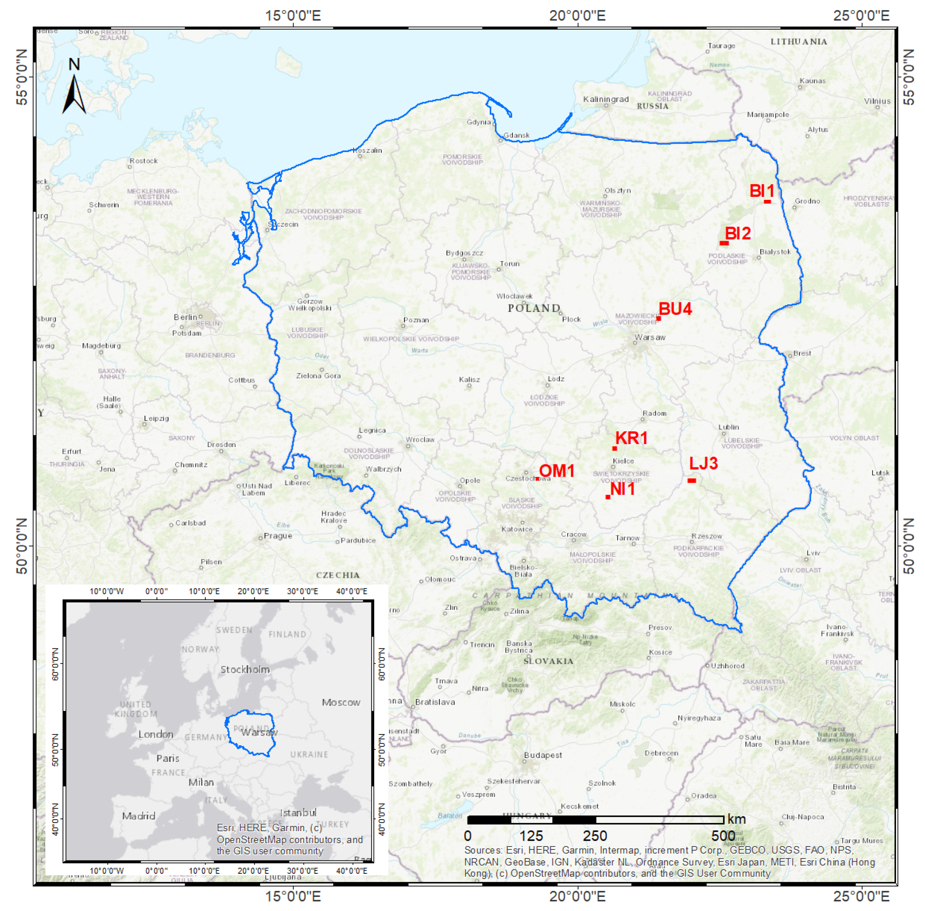
2. Project HabitARS Overview

The presented methodology is a result of the project HabitARS “The innovative approach supporting monitoring of non-forest Natura 2000 habitats, using remote sensing methods”. The main goal of the project was to develop an objective and repeatable method of identification of non-forest habitats and the main threats to these habitats, which are desiccation, secondary succession and encroachment of invasive alien and expansive domestic plant species, using remote sensing methods.

The project was carried out in 37 locations across Poland. The research areas have been selected in a way to consider the impact of different geographical conditions and local climatic conditions affecting the specificity of non-forest Natura 2000 habitats.

The project covered all 11 non-forest Natura 2000 habitats that require agricultural use in Poland, 10 alien invasive taxa, 8 domestic expansive taxa, and the species of trees and shrubs that are succession promotors in the researched habitats. A detailed description of the listed vegetation in provided on HabitARS project’s website: http://habitars.pl/en/o-projekcie/metodyka/ (accessed on 2 June 2021).

Research work on the identification of the succession process at non-forest Natura 2000 habitats was conducted in seven research areas (Figure 1) with diverse habitat conditions and levels of the threat of the succession process (

Table 1. Description of the Natura 2000 sites studied.

Natura 2000 Site (Code)	Acronym	Geographical Coordinates	Type of Natura 2000 Habitat Studied (Code)	Succession Species
Biebrza River Valley (PLH200008)	BI2, BI2	53°17′10″N; 22°37′45″E	Alkaline fens (7230)	Alnus glutinosa, Betula pubescens, Salix cinerea, Salix aurita, Salix rosmarinifolia
Lucynów-Mostówka Inland Dunes (PLH140013)	BU4	52°35′34″N; 21°27′30″E	European dry heaths (4030)	Pinus sylvestris, Betula pendula, Populus tremula, Prunus serotina
Nidziańska Refuge (PLH26003)	NI1	50°32′14″N; 20°30′42″E	Semi-natural dry grasslands and scrubland facies on calcareous substrates (Festuco-Brometalia) (6210)	Pinus sylvestris, Prunus spinosa, Rosa canina
Krasna Valley (PLH260001)	KR1	51°05′45″N; 20°37′00″E	European dry heaths (4030); Species-rich Nardus grasslands on siliceous substrates in mountain areas (6230); Molinia meadows on calcareous, peaty or clayey, silt-laden soils (Molinion caeruleae) (6410)	Salix cinerea, Salix aurita, Frangula alnus, Betula pendula, Pinus sylvestris
Janowskie Forests Ranges (PLH060031)	LJ3	50°43′0″N; 22°0′0″E	European dry heaths (4030); Transition mires and quaking bogs (7140)	Quercus robur, Populus tremula, Betula pendula, Betula pubescens, Pinus sylvestris
Olsztynsko-Mirowska Refuge (PLH240015)	OM1	50°0′45″N; 19°0′17″E	Xeric sand calcareous grasslands (Koelerion glaucae) (6120); Semi-natural dry grasslands and scrubland facies on calcareous substrates (Festuco-Brometalia) (6210)	Pinus sylvestris, Juniperus communis, Betula pendula, Prunus spinosa, Rhamnus cathartica, Crataegus spp., Cornus sanguinea, Corylus avellana

).

For each of the seven described research areas, a set of extensive tests was conducted with the aim of determining the best (quickest, simplest and most accurate) approach to mapping succession. These tests were done during the two research periods—of 2016 and 2017, each comprising of three (spring, summer and autumn) data acquisitions. In order to decide on the most favourable approach to calculating the spatial extent of trees and shrubs, data acquired on three different dates covering the growing period were compared (Figure A1 in Appendix A). Various approaches based on ALS data were tested, including those used for individual tree crown delineation [83,84,85,86], forests [87] and grasslands [88].

The possibilities of automating the processing of archival aerial photos aimed at determining the dynamics of the succession process were also studied, including the effectiveness of dense image matching algorithms and their parametrization [59,61,89], and granulometric maps [64]. The effectiveness of tree and shrub detection was also analysed by assessing the influence of the date and parameters of the aerial images acquisition and the dense image matching effects on the accuracy obtained (

Table A1. The accuracy assessment report of shrubs and trees extent determination (nDSM obtained using a dense image matching algorithm on archival aerial photos), OM1 study area.

nDSM Threshold Value	Parameter	Date of the Archival Photos Acquisition
		11 August 1971	30 May 1996	24 May 2003	29 April 2009	08 August 2015
	No. of polygons	831	1835	3580	4429	3019
1.0 m	OA	0.850	0.833	0.914	0.902	0.926
	Recall	0.963	0.854	0.877	0.774	0.964
	Precision	0.422	0.522	0.794	0.923	0.863
	Kappa	0.512	0.546	0.776	0.772	0.848
	F1-score	0.587	0.648	0.833	0.842	0.911
1.25 m	OA	0.872	0.886	0.919	0.902	0.936
	Recall	0.958	0.814	0.865	0.765	0.955
	Precision	0.461	0.646	0.816	0.932	0.890
	Kappa	0.556	0.650	0.786	0.770	0.867
	F1-score	0.622	0.720	0.840	0.840	0.921
1.5 m	OA	0.889	0.911	0.922	0.901	0.939
	Recall	0.950	0.781	0.854	0.756	0.945
	Precision	0.498	0.739	0.832	0.939	0.904
	Kappa	0.595	0.704	0.791	0.767	0.873
	F1-score	0.653	0.759	0.843	0.837	0.924
1.75 m	OA	0.903	0.922	0.923	0.900	0.942
	Recall	0.934	0.755	0.844	0.747	0.937
	Precision	0.535	0.802	0.844	0.944	0.916
	Kappa	0.630	0.731	0.793	0.763	0.878
	F1-score	0.653	0.778	0.844	0.834	0.926
2.0 m	OA	0.903	0.927	0.924	0.898	0.942
	Recall	0.886	0.734	0.833	0.740	0.928
	Precision	0.588	0.842	0.854	0.948	0.924
	Kappa	0.663	0.742	0.793	0.760	0.878
	F1-score	0.707	0.748	0.844	0.831	0.926

and

Table A2. Area of omission (EO) and area of commission (EC) [in hectares] report of shrubs and trees extent determination (nDSM obtained using a dense image matching algorithm on archival aerial photos), OM1 study area.

nDSM Threshold Value	Parameter	Date of the Archival Photos Acquisition
		11 August 1971	30 May 1996	24 May 2003	29 April 2009	08 August 2015
1.0 m	EO	0.43	3.13	3.70	9.21	1.64
	EC	15.66	12.24	5.46	1.70	5.73
	EO + EC	16.09	15.37	9.16	10.91	7.37
1.25 m	EO	0.49	4.02	4.06	9.62	2.05
	EC	13.13	6.76	4.75	1.50	4.53
	EO + EC	13.62	10.78	8.81	11.12	6.58
1.5 m	EO	0.58	4.77	4.39	9.99	2.51
	EC	11.04	4.08	4.24	1.35	3.87
	EO + EC	11.62	8.85	8.63	11.34	6.38
1.75 m	EO	0.79	5.34	4.70	10.33	2.86
	EC	9.22	2.72	3.86	1.25	3.38
	EO + EC	10.01	8.06	8.56	11.58	6.24
2.0 m	EO	1.45	5.81	5.01	10.66	3.27
	EC	8.90	2.01	3.52	1.16	3.03
	EO + EC	10.35	7.82	8.53	11.82	6.30
Area of the reference mask		13.66	22.58	30.95	42.88	49.78

in Appendix A). The relationship between the parameters characterising succession trees and shrubs (e.g., species, height, diameter, and density of the crown) and the possibility of their automatic detection was also studied [59].

Within the research on differentiating species, the accuracy and processing time of classifications made using different classifiers (e.g., random forest, spectral angle mapper, support vector machine), different ALS point cloud classification methods [90], input products (hyperspectral data-based, LiDAR data-based and the combination of both), different dimensionality reduction methods (e.g., minimum noise fraction, principal component analysis, vegetation indices), different spatial resolutions of hyperspectral data [91] and reference data processing approaches were compared [82,92] (

Table A3. Accuracy assessment report of the influence the spatial resolution of the hyperspectral data has on the results of the species classification (var 1—reference polygons were buffers with a crown diameter of a tree or shrub, var 2—reference polygons were buffers limited using the height criterion, the presence of vegetation and shadows, var 3—same as var 2, but characterized by more stringent threshold values).

Species	Spatial Resolution	1 m	1 m	1 m	0.5 m	0.5 m	0.5 m
	Variant	var 1	var 2	var 3	var 1	var 2	var 3
	Kappa	0.55	0.57	0.67	0.56	0.62	0.68
Betula pendula	F1	0.60	0.65	0.78	0.62	0.68	0.79
Salix spp.	F1	0.80	0.83	0.87	0.80	0.86	0.87
Frangula alnus	F1	0.57	0.56	0.75	0.58	0.61	0.76
Pinus sylvestris	F1	0.70	0.68	0.76	0.70	0.76	0.80
Quercus robur	F1	0.55	0.72	0.75	0.55	0.69	0.72
Pyrus communis	F1	0.28	0.21	0.27	0.25	0.27	0.33
Padus serotina	F1	0.16	0.19	0.10	0.17	0.20	0.15
	Kappa	0.51	0.54	0.65	0.52	0.58	0.66
Betula pendula	F1	0.52	0.51	0.66	0.56	0.57	0.69
Rhamnus catharticus	F1	0.49	0.53	0.59	0.50	0.54	0.64
Prunus spinosa	F1	0.67	0.71	0.82	0.63	0.71	0.78
Pinus sylvestris	F1	0.58	0.61	0.72	0.59	0.69	0.76
Quercus robur	F1	0.49	0.10	0.00	0.46	0.04	0.02
Pyrus communis	F1	0.49	0.47	0.69	0.46	0.47	0.62
Padus serotina	F1	0.56	0.60	0.69	0.57	0.62	0.69
Juniperus communis	F1	0.62	0.62	0.69	0.64	0.69	0.68
Corylus avellana	F1	0.54	0.63	0.72	0.51	0.66	0.74
Robinia pseudoacacia	F1	0.62	0.69	0.75	0.65	0.71	0.78
Cornus sanguinea	F1	0.64	0.67	0.70	0.62	0.67	0.74
Cratageus_spp.	F1	0.47	0.51	0.68	0.47	0.57	0.61

in Appendix A). Similarly to the extent of the succession, the influence of the data acquisition time was also studied [82,93] (

Table A4. The report of the influence the data acquisition date has on the accuracy of species classification.

BI2 Study Area
Species		spring 22 June 2017	summer 12 August 2017	autumn 29 September 2017
	Kappa	0.52	0.57	0.58
Salix cinerea	F1	0.79	0.77	0.79
Pinus sylvestris	F1	0.74	0.75	0.77
Alnus glutinosa	F1	0.51	0.57	0.65
Betula pubescens	F1	0.36	0.49	0.42
BU4 Study Area
Species		spring 28 May 2017	summer 10 July 2017	autumn 9 September 2017
	Kappa	0.79	0.71	0.72
Pinus sylvestris	F1	0.9	0.63	0.78
Betula pendula	F1	0.74	0.78	0.69
Padus serotina	F1	0.92	0.91	0.89
Populus tremula	F1	0.82	0.69	0.74
NI1 study area
Species		spring 18 May 2017	summer 30 July 2017	autumn 27 September 2017
	Kappa	0.52	0.68	0.73
Rhamnus catharticus	F1	0.37	0.33	0.48
Pinus sylvestris	F1	0.75	0.74	0.78
Robinia pseudoacacia	F1	0.65	0.82	0.83
Prunus spinosa	F1	0.71	0.83	0.86
Cratageus_spp.	F1	0.48	0.44	0.33
Cornus sanguinea	F1	0.59	0.84	0.86
OM1 study area
Species		autumn 10–13 September 2016	spring 9 June 2017	summer 11 August 2017
	Kappa	0.53	0.61	0.61
Betula pendula	F1	0.78	0.75	0.76
Rhamnus catharticus	F1	0.41	0.45	0.49
Pinus sylvestris	F1	0.52	0.7	0.7
Juniperus communis	F1	0.48	0.57	0.61
Robinia pseudoacacia	F1	0.71	0.77	0.77
Cratageus_spp. + Pyrus communis	F1	0.43	0.61	0.53
Prunus spinosa	F1	0.68	0.76	0.71
Corylus avellana	F1	0.61	0.72	0.66
Padus serotina	F1	0.44	0.39	0.44

in Appendix A). Finally, the critical botanical characteristics of the research objects affecting the effectiveness of succession species mapping were also analysed [92].

3. Proposed Methodology of Secondary Succession Process Identification—Result of the Project

The objective of the project was to develop a succession process identification methodology for monitoring non-forest Natura 2000 habitats with remote sensing techniques. The prepared methodology consists of six steps (Figure 2):

• Step 1—Data acquisition and pre-processing.
• Step 2—Determining the spatial extent of the potential succession of trees and shrubs.
• Step 3—Determining the level of potential threat of succession for the whole analysed area.
• Step 4—Determining the level of threat of succession for selected individual habitats based on area and height characteristics.
• Step 5—Determining the level of threat of succession for selected individual habitats based on species composition.
• Step 6—Determining the succession dynamics for selected individual habitats.

3.1. Step 1—Data Acquisition and Pre-Processing

Flight and field campaigns are preceded by a preliminary recognition of the study area, which is carried out based on available materials (e.g., remote sensing data, protection plans, reports). From their analysis it can be decided if succession is a threat to the area and, if so, which succession and herein named background species are present there. Background species are tree and shrub species that do not form the process of succession, but still cover a substantial part of the study area. They therefore need to be included in the classification process in order to correctly delineate the spatial extent of succession species. An important goal of preliminary recognition is also to indicate tall species of herbaceous plants (e.g., reeds, sedges) which are present in the analysed area. As these are of a similar height to shrubs and undergrowth of trees, they may potentially mix with them, and therefore cause an overestimation or underestimation of the area of succession.

As a result of the preliminary recognition, knowledge is gathered about: types of habitats threatened by encroaching trees and shrubs; key species for the secondary succession process together with information on the nature of their occurrence in space and dominant features (e.g., height, crown density); and the stages of the advancement of secondary succession in particular parts of the area. All of this information is then used to properly plan the field and flight campaigns. Detailed guidelines for the field campaign are described in Appendix B.

The field measurements are coupled with the flight campaign. The remote sensing data collected include high-resolution hyperspectral imagery and fullwave LiDAR data acquired simultaneously from the common, specially prepared aerial platform built by MGGP Aero. Acquiring both types of data at the same time avoids problems resulting from changes in vegetation cover due to phenology as well as various human activities, and therefore facilitates subsequent data fusion. The technical parameters of the sensors and both data types are shown in

Table 2. Technical parameters of the sensors used, and the remote sensing data obtained using HabitARS platform.

Technical Parameters	Sensor Type
	Airborne Laser Scanner (FWF)	Hyperspectral Camera HySpex
	Riegl LMS-Q680i	VNIR-1800	SWIR-384
Flight altitude AGL [m]	500
Point density [pt/m2]	7	-	-
Spatial resolution [m]	-	0.5	1
Spectral resolution	1.55 µm	430 bands encompassing 0.4–2.4 µm spectral range
Spectral sampling [nm]	-	3.26	5.45
FOV max [degrees]	60	34	32
Scan line overlap area [%]	62.7	30	30
Scan line overlap width [m]	855	450	450

.

In the next step, the data obtained from the HabitARS platform are processed to generate standardised products—hyperspectral mosaic, minimum noise fraction (MNF) components [94], vegetation indices, crown height model (CHM) and other LiDAR-based raster products. A detailed description of the HabitARS platform and the method of preparing individual products can be found in [95].

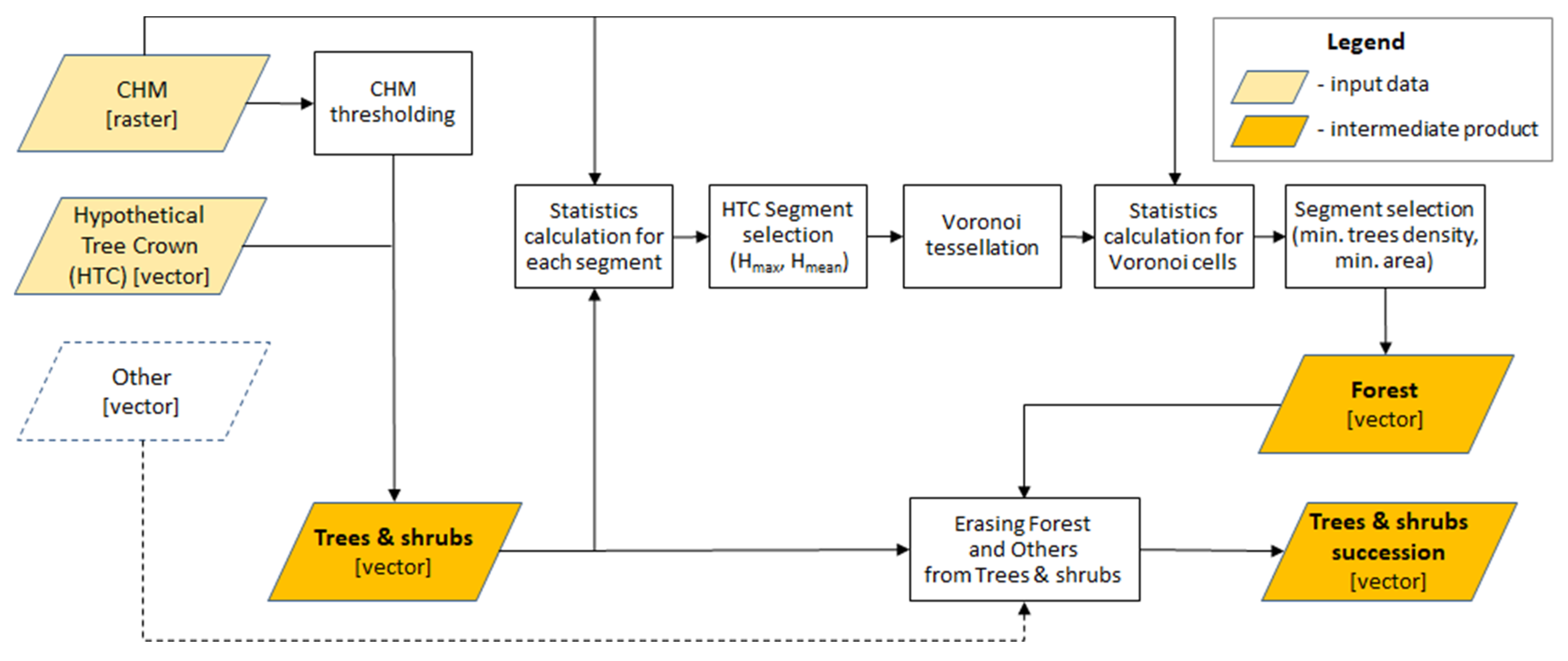
3.2. Step 2—Determining the Spatial Extent of the Potential Succession of Trees and Shrubs

The process of determining the spatial extent of shrubs and undergrowth of trees potentially representing succession consists of two steps. First, the extent of trees and shrubs in the area of study is determined. Then, it is limited by two other layers—the extent of compact forest stands and other types of vegetation that are unrelated to succession. The resulting difference defines the extent of a potential succession for a given area.

In order to create a layer representing the extent of trees and shrubs, all pixels with a height larger than a defined threshold are selected using a CHM. The threshold value is determined by a botanist with knowledge about a specific habitat. As the optimal threshold value depends on both the habitat and the specifics of the study area, the proposed workflow assumes that multiple thresholds could be used for a single study area—different for each habitat. In the next step the extent of trees and shrubs is filtered in order to remove vegetation that is unrelated to succession (for example: green spaces in urban areas, orchards, tall herbaceous plants). The mask used can be created from different external spatial databases (e.g., in Poland BDOT10k country wide database of topographical objects with spatial resolution adequate to a 1:10,000 topographic map). Finally, the spatial extent of forest stands is excluded from the created layer. In order to delineate these areas, a modified method based on Eysn et al. [96] is used. Instead of detecting single treetops, polygons representing hypothetical single tree crowns are used as input data. This polygonal vector layer is the result of watershed segmentation for the single tree delineation algorithm implemented in Toolbox for LiDAR Data Filtering and Forest Studies (TIFFS) [84]. Additionally, the percentage value of crown coverage in the Voronoi cell that is used for the qualification of which hypothetical single tree crowns should be included in the forest area is calculated with Voronoi tessellation instead of triangulation, which was originally proposed by Eysn et al. [96].

A scheme for determining the spatial extent of trees and shrubs potentially forming secondary succession is presented in Figure 3.

As a result of the implementation of the entire procedure, four different extents are provided: all trees and shrubs, forests, and the extent of trees and shrubs potentially causing succession. An example of the resulting map is presented in Figure S1 of the Supplementary Materials.

3.3. Step 3—Determining the Level of Potential Threat of Succession for the Whole Analysed Area

In the next step of the analysis of the secondary succession process, the level of the herein named potential threat of succession is determined, which is defined by the area and height of understory layer of small trees and shrubs present within the whole study area.

The character of this potential threat is defined by a set of landscape metrics describing the properties of the area of succession based on its spatial extent layer obtained in step 2, and height metrics calculated based on the CHM layer obtained in step 1. This set of metrics was specifically selected so that together they characterise the structure of succession in a comprehensive way, at the same time providing objective results—in the form of numbers. The metrics proposed for use in the methodology are described in detail in Appendix C (

Table A5. Metrics characterising the area and the height structure of shrubs and trees patches in the grid or tura 2000 habitat.

Metrics Name	Formula	Units	Metric‘s Description/Interpretation
Metrics characterising the area of shrub and tree patches
Area Metrics
Total area of patches of shrubs and trees in the grid or Natura 2000 habitat	$TA={\displaystyle {\displaystyle \sum }_{i=1}^n}{a}_i$ ai—area of the individual patch of shrubs and trees n— number of patches of shrubs and trees	m2	TA is a measure of landscape composition. It shows to what extent the analysed landscape (grid or Natura 2000 habitat) is comprised of shrub and tree patches. This is the basic parameter describing the encroachment of trees and shrubs into a given area. Its analysis should be combined with the analysis of other metrics. TA takes values greater than or equal to 0. Value 0 means that there are no shrubs and trees in the analysed grid. The upper limit of the value is only limited by the grid size area.
Percentage share of the area covered by patches of shrubs and trees within the grid or Natura 2000 habitat	$\%TA=\frac{TA}{A}·100$ A—area of the analysed grid or Natura 2000 habitat	%	%TA quantifies the proportional abundance of patches of shrubs and trees in the analysed landscape (grid or Natura 2000 habitat). This is a basic parameter describing the encroachment of trees and shrubs into a given area. %TA takes values in the range 0–100. Value 0 means that there are no shrubs and trees in the analysed grid or Natura 2000 habitat. A value of 100 means that the entire landscape consists of only trees and shrubs.
Mean size (area) of patches of shrubs and trees in the grid or Natura 2000 habitat	$MSP=\frac{TA}{n}$	m2	MSP is a metric informing about the average size of patches of shrubs and trees in the analysed area (grid or Natura 2000 habitat). The lower the value of the metric, the smaller (on average) the patches of trees and shrubs. In the case of large and sparse patches of high trees and shrubs, it can be assumed that the succession process is not progressing. On the other hand, a large number of small-area and low-height tree and shrub patches may indicate succession in the analysed area. MPS takes values greater than or equal to 0. The upper limit of the value is limited by the size of the analysed area.
Standard deviation of size of shrub and tree patches (area) in the grid or Natura 2000 habitat	$SDP=\sqrt{\frac{{{\displaystyle \sum }}_{i=1}^n{[a_i-MSP]}^2}{n}}$	m2	SDP measures absolute variation in patch size and is affected by the average patch size. It is a measure of the variation in the size of patches of trees and shrubs in the analysed area (grid or Natura 2000 habitat). The higher SDP value, the greater the variation in the size of tree and shrub patches in this area. High value means that there are patches of trees and shrubs of various sizes. In the case of low values of SDP, the area is characterized by trees and shrubs of similar size. This metric, together with other ones (e.g., MSP, NumP, hmean), allows us to assess whether succession of trees and shrubs is present in a given area. SDP takes values greater than or equal to 0.
Edge Metrics
Total Edge—the sum of the lengths of all edge of shrub and tree patches in the grid or Natura 2000 habitat	$TE={\displaystyle {\displaystyle \sum }_{i=1}^n}{e}_i$ ei—lengths of edge of shrub and tree patches	m	TE is the sum of the lengths of the borders of all patches of trees and shrubs in the analysed area (grid or Natura 2000 habitat). It is an absolute index, and in the case of comparing areas of different sizes, it is of less utility than border density (ED), described below. However, when analysing areas of a similar size or analysing the same area in subsequent periods, it may be very useful. TE gives information about the complexity of shapes of tree and shrub patches. The more complicated the shape, the longer the boundaries are. TE takes values greater than or equal to 0. Value 0 means that there are no patches of trees and shrubs in the analysed area.
Edge Density—the sum of the lengths of all edge of shrub and tree patches, divided by the total grid or Natura 2000 habitat area	$ED=\frac{{{\displaystyle \sum }}_{i=1}^n{e}_i}{A}$	m/m2	ED is a relative measure related to the area of the analysed area—in the grid or Natura 2000 habitat. It enables the comparison of areas with different sizes. ED indirectly indicates of the complexity of shapes of patches within the analysed area. More complex shapes with a smaller area of trees and shrubs patches at the same time indicate the succession process. In the case of forest, TE will be lower, and also TA will be lower. ED takes values greater than or equal to 0. Value 0 means no trees and shrubs are present in the analysed area.
Subdivision Metrics
Number of patches of shrubs and trees in the grid or Natura 2000 habitat	$NumP=n$	-	NumP is a simple measure of the degree of division or fragmentation of the analysed area (grid or Natura 2000 habitat). In general, the information on the number of patches has limited interpretative value as it does not provide information about the analysed area, distribution or density of patches. However, in the case of a comparative analysis of the area NumP can be a useful metric for interpreting the level of succession of trees and shrubs, especially when it is analysed simultaneously with other metrics (e.g., TA, TE, %SS). A large number of tree and shrub patches may indicate a progressive succession process, which can be used in the case of time-series analyses. The lowest possible values of NumP is 0 and has no upper boundary.
Shape Metrics
Area-weighted mean patch (of shrubs and trees) fractal dimension, calculated in the grid or Natura 2000 habitat	$AWMPFD=\frac{{{\displaystyle \sum }}_{i=1}^n\left(\frac{2 \ln (0.25 e_i}{\ln (a_i)}\right)}{n}·\left(\frac{a_i}{{{\displaystyle \sum }}_{i=1}^n{a}_i}\right)$	-	AWMPFD is the surface weighted average fractal dimension, which indicates the complexity of shapes of tree and shrub patches in the study area (grid or Natura 2000 habitat). It is a relative metric taking into account the size of the analysed areas. The higher the value of this metric, the greater the complexity of the shape of trees and shrubs patches in this area. This, in turn, may indicate the intensification of the process of succession of trees and shrubs, in particular when we compare the results of the analysis in subsequent periods.
Metrics characterising the height structure of shrubs and trees
Average height of shrubs and trees in the grid or Natura 2000 habitat	$h_{mean}=\frac{{{\displaystyle \sum }}_{i=1}^n{h}_i}{TA}$	m	The height of trees and shrubs makes it possible to assess what kind of vegetation is present in the studied area (grid or Natura 2000 habitat). However, both the average and maximum height of trees and shrubs should not be considered on their own, without taking into account the area metrics. When there are many patches of low trees and shrubs with a small area, it is highly probable that the succession process is observed in this area. If there are a few high-height patches of trees and shrubs, it is a group of trees.
Maximum height of shrubs and trees in the grid or Natura 2000 habitat	$h_{mean}=\frac{{{\displaystyle \sum }}_{i=1}^n{h}_i}{TA}$	m
Standard deviation of the height of shrubs and trees in the grid or Natura 2000 habitat	$h_{SD}=\sqrt{\frac{{{\displaystyle \sum }}_{i=1}^n{[h_i-h_{mean}]}^2}{TA}}$	m	Standard deviation of the height of shrubs and trees (hSD), calculated for the studied area (grid or Natura 2000 habitat), informs about the variation in the height of trees and shrubs. In the case of low hSD values, shrubs and trees in the study area have similar heights. When hSD value is high, there are trees and shrubs of various heights in the analysed area. In such a case, the area metrics should also be analysed, as it may indicate a succession process.

).

Firstly, the metrics are calculated for a grid of squares (in the herein described methodology with a size of 25 × 25 m²), as shown in Figure 4. Then, specially defined criteria (

Table 3. The criteria used to define the levels of potential threat of succession for the whole analysed area.

Metric	Level of Threat
	No	Small	Medium	High
Percentage share of the area covered by patches of shrubs and trees within the grid [%]	<0–5)	(5;10>	(10;25>	>25
The total length of the boundaries of patches of shrubs and trees within the grid in which the percentage of shrubs and trees is less than or equal to 95% [m]	<1	<1;100>	(100;250>	>250

) are applied to these metrics. This means that the metrics are given thresholds defining logical conditions, which enable different secondary succession threat levels to be indicated. Based on this information, a map of the potential threat of the succession process is prepared for the study area. An example of such a map is presented in Figure S2 of the Supplementary Materials.

The final level of threat for the analysed area is defined as low if all metrics indicate a small level of threat or no threat. A medium level occurs in the situation when at least one metric shows a medium level of threat and none of them indicates a high one. Finally, a high level of threat for the area occurs when at least one metric shows a high threat level.

3.4. Step 4—Determining the Level of Threat of Succession for Selected Individual Habitats Based on Area and Height Characteristics

After assessing the level of potential threat for the whole area, individual habitats are examined to obtain detailed information. Habitat threat level analysis consists of two elements—determining the herein named internal and external threat. The internal threat refers to the area and height of shrubs and undergrowth of trees located within the habitat, while the external threat refers to the vegetation present in the immediate vicinity of the habitat. Similarly to the potential threat described earlier, the level of internal and external threat is determined using specially defined criteria that are applied to a set of landscape metrics.

The metrics used to determine the level of internal threat characterising the habitat are calculated according to the diagram in Figure 5 and include metrics characterising the area and the height of shrub and tree patches (Table 3). In addition, to perform a more detailed analysis of the structure of patches of trees and shrubs in a habitat, more metrics characterising the area and the height structure of shrub and tree patches can be calculated (Table A5 in Appendix C).

After calculating the area and height metrics, and applying the appropriate criteria (their definition may be different for individual Natura 2000 habitats) (

Table 4. The criteria used to define the levels of internal threat of succession for selected individual habitats.

Metric	Level of Threat
	No	Small	Medium	High
Percentage of the area of patches of shrubs and trees in the analysed habitat [%]	<0–1)	<1;10>	(10;25>	>25
Average height of shrubs and trees in the analysed habitat [m]	-	<0;1>	(1;3>	>3
Percentage share of succession species in the area of shrubs and trees (species of succession + other trees and shrubs species = 100%) in the analysed habitat	<0;5)	<5;30>	(30;60>	>60

), a map of the internal threats to habitats from the process of succession can be prepared. An example of such a map is presented in Figure S3 in the Supplementary.

The presented criteria were formulated based on the rules of habitat state valorisation and indices characterising the specific structure and function of the habitat defined in the methodological guide entitled “Monitoring of natural habitats” [1,97] and botanical expert knowledge. Similarly to the potential threat, the final level of internal threat for the analysed habitat is defined as low if all metrics indicate a small level of threat or no threat. A medium level occurs in the situation when at least one metric shows a medium level of threat and none of them indicates a high one. Finally, a high level of threat for the habitat occurs when at least one metric shows a high threat level.

The area of trees and shrubs located near the habitat, in a buffer of up to 50 m from its boundaries, is understood as an external threat to habitats from the succession process. The buffer size was adopted after Michalska-Hejduk [98]. Metrics characterising the neighbourhood of the habitat are calculated according to the diagram in Figure 6 and include the area and distance parameters of tree and shrub patches in a buffer of 50 m from the border of the habitat. A detailed description of the individual metrics is provided in

Table A6. Metrics characterising the area and the height structure of shrub and tree patches in a buffer of 50 m from the border of Natura 2000 habitat.

Metrics Name	Formula	Units	Metric’s Description/Interpretation
Metrics characterising the area of shrub and tree patchesin a buffer of 50 m from the border of the Natura 2000 habitat
Area Metrics
Sum of the area of patches of trees and shrubs in a buffer of 50 m from the border of the habitat	$T{A}_{buffer}={\displaystyle {\displaystyle \sum }_{i=1}^{n_{buffer}}}{a}_i$ ai—area of individual shrub and tree patches in a buffer of 50 m from the border of the habitat nbuffer—number of patches of shrubs and trees in a buffer of 50 m from the border of the habitat	m2	TAbuffer metrics shows to what extent the analysed buffer is comprised of shrub and tree patches. The TAbuffer takes values greater than or equal to 0. Value 0 means that there are no shrubs and trees in the analysed buffer. The upper limit of the value is only limited by the size of the buffer area. If there are many trees and shrubs in the buffer around a Natura 2000 habitat, and they are successive species, then TA shows the presence of threat from the succession process in the habitat.
Percentage of the area of patches of trees and shrubs in a buffer of 50 m from the border of the habitat	$\%T{A}_{buffer}=\frac{T{A}_{buffer}}{A_{buffer}}·100$ Abuffer—area of a buffer of 50 m from the border of a habitat	%	%TAbuffer metric quantifies the proportional abundance of patches of shrubs and trees in the buffer from the border of the analysed Natura 2000 habitat. It is the basic parameter describing the presence of trees and shrubs in the buffer around the Natura 2000 habitat. %TAbuffer takes values in the range 0–100. Value 0 means that there are no shrubs and trees in the buffer from the border of the analysed Natura 2000 habitat. A value of 100 means that the buffer contains only trees and shrubs. If these are successive species, the threat to the conservation of the habitat will be high.
Percentage share of succession species in the area of shrubs and trees (species of succession + other tree and shrubs species = 100%) in a buffer of 50 m from the habitat	$\%S{S}_{buffer}=\frac{S{S}_{buffer}}{T{A}_{buffer}}·100$ SSbuffer—area of the succession species		This metric shows how large the part of the buffer area around the habitat consisting succession species is. The higher the value of this metric, the greater the threat to the preservation of the habitat. %SSbuffer takes values between 0–100. Value 0 means that there are no species of succession in the buffer from the border of the analysed Natura 2000 habitat. A value of 100 means that the buffer contains only species of succession.
Mean size (area) of patches of shrubs and trees in a buffer of 50 m from the habitat	$MS{P}_{buffer}=\frac{T{A}_{buffer}}{n_{buffer}}$	m2	This is a metric informing about the average size of patches of shrubs and trees in a buffer of 50 m from the analysed Natura 2000 habitat. The lower the value of the metric, the smaller the patches of trees and shrubs in the buffer. In the case of large-area, high-height trees and shrubs, it can be presumed that there are forest stands in the buffer. In contrast, the large number of small-area and low-height tree and shrub patches may indicate succession in the area under study. MPSbuffer takes values greater than or equal to 0. The upper limit of the value is limited by the size of the analysed buffer.
Standard deviation of size of shrub and tree patches (area) in in a buffer of 50 m from the habitat	$SD{P}_{buffer}=\sqrt{\frac{{{\displaystyle \sum }}_{i=1}^n{[a_i-MS{P}_{buffer}]}^2}{n_{buffer}}}$	m2	SDPbuffer measures absolute variation in patch sizes and is affected by the average patch size. It is a measure of the variation in the size of patches of trees and shrubs in the buffer around the analysed Natura 2000 habitat. The higher SDPbuffer value, the greater the variation in the size of patches of trees and shrubs in a buffer. This means that there are patches of trees and shrubs of various sizes. In the case of small SDPbuffer values, patches of trees and shrubs are of similar size. This metric with other ones (e.g., MSPbuffer, NumPbuffer) allows us to assess if succession is present in the buffer. SDPbuffer takes values greater than or equal to 0.
Subdivision Metrics
Number of patches of shrubs and trees in in a buffer of 50 m from the habitat	$Num{P}_{buffer}=n_{buffer}$	-	NumPbuffer is a simple measure of the degree of division or fragmentation of the analysed area and may indicate changes taking place. The more patches of trees and shrubs in the buffer around the analysed habitat, the greater is the potential threat of trees and shrubs entering the Natura 2000 site. A combined analysis with %TAbuffer and %SSbuffer metrics will indicate whether the threat is real. NumPbuffer is 0 and has no upper boundary.
Metrics characterising the distance of tree and shrub patches relative to the border of the habitat (in a buffer of 50 m from the border of the habitat)
Minimum distance of the tree or shrub patch border to the border of the habitat in a buffer of 50 m from the habitat	$min{D}_{buffer}=min\left(d_i\right)$ di—the distance of the i-th patch of trees and shrubs from the border of the habitat	m	The distance of trees and shrubs from the Natura 2000 habitat is one of the measures of the threat of the succession process. If succession trees and shrubs occur in the neighbourhood of the Natura 2000 habitat, there is a greater risk of spreading succession species in its area than if they are located at considerable distances from the boundaries of the habitat. If the values of the minDbuffer and meanDbuffer are similar, and there are many trees and shrubs around the habitat, it may mean that there is a threat of succession.
Mean distance of the tree or shrub patch border to the border of the habitat in a buffer of 50 m from the habitat	$mean{D}_{buffer}=\frac{{{\displaystyle \sum }}_{i=1}^{n_{buffer}}{d}_i}{n_{buffer}}$	m

in Appendix C.

After calculating the area and distance metrics and applying the appropriate criteria (their definition may be different for individual Natura 2000 habitats) (

Table 5. The criteria used to define the levels of external threat of succession for selected individual habitats.

Metric	Level of Threat
	No	Small	Medium	High
Percentage of the area of patches of trees and shrubs in a buffer of 50 m from the border of the habitat [%]	<0–5)	<5;10>	(10;50>	>50
Mean distance of the tree or shrub patch border to the border of the habitat in a buffer of 50 m from the habitat [m]	-	>25	(10;25>	<0;10>
Percentage share of succession species in the area of shrubs and trees (species of succession + other trees and shrubs species = 100%) in a buffer of 50 m from the habitat	<0;5)	<5;30>	(30;60>	>60

), a map of the external threat to habitats from the process of succession can be prepared. An example of such a map is presented in Figure S4 in the Supplementary Materials.

The threshold values for the presented criteria are a result of a set of experiments conducted in cooperation with botany experts. Similarly to the two threats mentioned above, the final level of external threat for the analysed habitat is defined as low if all metrics indicate a small level of threat or no threat. A medium level occurs in the situation when at least one metric shows a medium level of threat, and none of them indicates a high one. Finally, a high level of threat for the habitat occurs when at least one metric shows a high threat level.

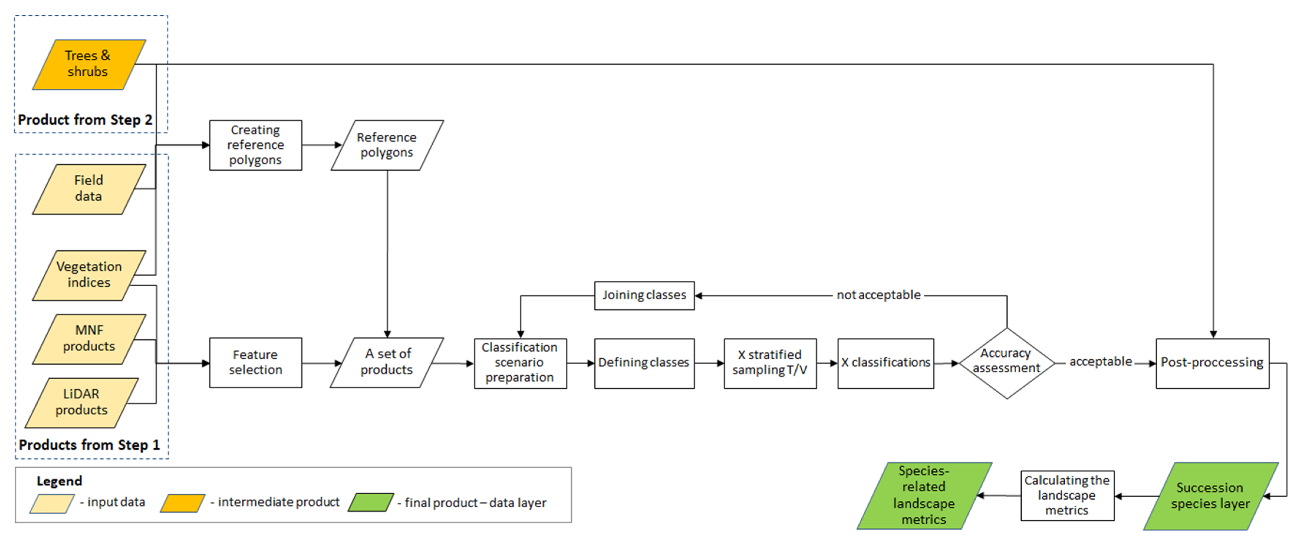
3.5. Step 5—Determining the Level of Threat of Succession for Selected Individual Habitats Based on Species Composition

The next step of the methodology aims to provide a more detailed examination of the analysed habitats by identifying species involved in the process of succession. This information is important, as it determines the type of active protection that is needed. The results of this step include the spatial extent, thus the location and area, of succession species, as well as additional landscape metrics characterising internal and external threats to the habitat. This step includes the following substeps (Figure 7):

• Creating reference polygons;
• Applying a feature selection algorithm to the remote sensing products;
• Iterative classification and determining the spatial extent of individual species;
• Calculating the landscape metric.

As mentioned above, in the first substep, the reference polygons are created using a semi-automatic algorithm that was developed within the project HabitARS (described in detail in Osińska-Skotak et al. [82]). The procedure is based on the spatial extent of trees and shrubs layer developed in step 2, the normalized difference vegetation index (NDVI) and botanical field measurements. It starts with determining the spatial relationship between each measurement point and the trees/shrubs present nearby. It is possible to successfully match these because field data are collected only for isolated specimens or groups of specimens of the same species. Next, the tree/shrub reference objects determined are the subject of pixel-level analysis using NDVI. Finally, the spatial extent of each polygon is limited in order to remove the boundary, mixed pixels and therefore create pure spectral signatures.

In the second substep, the feature selection algorithm—recursive feature elimination [99] is applied to the set of standardised remote sensing products developed in step 1 of the methodology—MNF products, vegetation indices and geometry-related indices calculated based on LiDAR data. Here, the feature selection is intended to reduce the volume of data and at the same time find the optimal set of features (layers) enabling differentiation of the species of interest.

In the third substep, the species classification is done based on the prepared reference polygons and the set of selected remote sensing products. The polygons are divided into two groups—training and validation sets, by stratified sampling, taking into account, e.g., the height, crown diameter and crown density of specimens. The draw is done 50 times to check the stability of the result. Having done this, the classification is performed using the random forest algorithm [100]. The accuracy of the product is assessed by analysing the classification error matrix, Cohen’s kappa coefficient and F1-score for each species, as well as based on the opinion of an expert in the field of botany. The classification process has an iterative nature—if the assessment of classifications indicates too little separation of some species or groups of species, in the next iteration they are aggregated into one class. In order to evaluate the separability of species in the remote sensing feature space, homogeneity analysis can also be done using the t-distributed stochastic neighbour embedding method (t-SNE), which enables the visualisation of high-dimensional data in a low-dimensional space in the form of a two- or three-dimensional graph [101]. A satisfactory result of the classification is characterised by an appropriate statistical accuracy (measured with the Cohen’s Kappa coefficient and F1—above 0.7) and is approved by a specialist in botany. Finally, the chosen classification image is post-processed by limiting the obtained result to the spatial extent of succession. Finally, additional landscape metrics characterising the internal and external threat to the habitat are calculated based on the classification product.

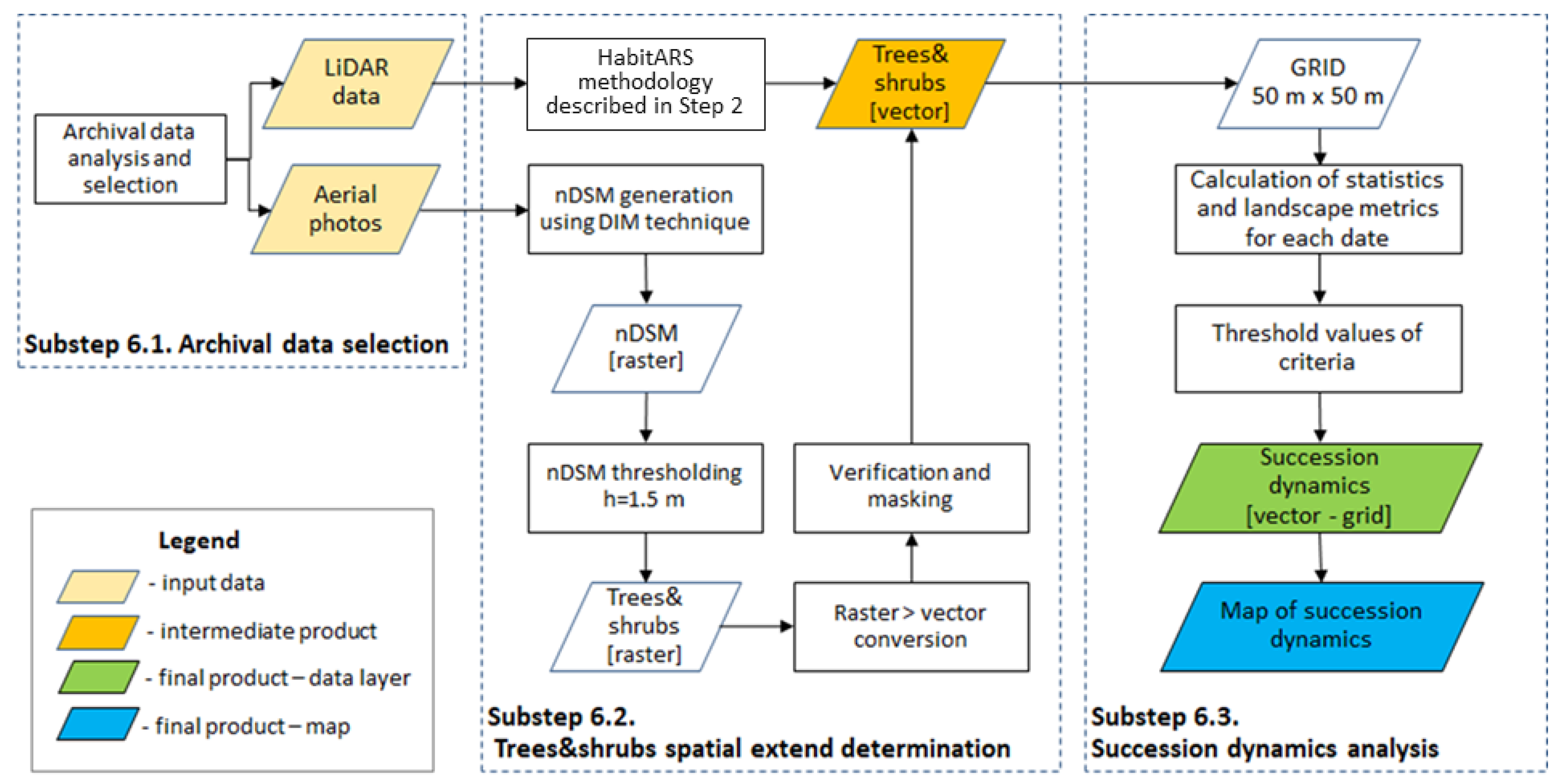
3.6. Step 6—Determining the Succession Dynamics for Selected Individual Habitats

The last step of the developed methodology aims at determining the succession dynamics (Figure 8).

In order to analyse the dynamics of succession using archival data, it is first necessary to review and inventory available archival materials—aerial photographs and LiDAR data, and assess whether:

• They were acquired during the leaf-on season, allowing data acquisition presenting fully developed crowns of trees and shrubs (in Poland it is from the second half of May to the end of September/beginning of October);
• In the case of LiDAR data, the scanning density is at least 7 pt/m²;
• In the case of archival aerial photographs, their scale is at least 1:13,000 (in relation to analogue images) or GSD ≤ 25 cm (in relation to images acquired with digital cameras) and whether they are of good radiometric quality (good contrast and large range of values) shades/colours.

Depending on what kind of archival aerial data are available, the scheme of their processing will differ in the level of complexity. In the case of obtaining data from airborne laser scanning, further stages of the analysis are carried out analogously to what has been described in Step 2. If archival aerial photographs in analogue form were collected, they first need to be scanned, then—in the case of aerial photographs for which the camera parameters are unknown—it is necessary to recreate the camera’s metric, as well as to determine external orientation parameters. With oriented images, generating point clouds using dense image matching techniques can be started. As a result of the research carried out as part of the HabitARS project, it turned out that point clouds of the best quality, i.e., the highest density, for detection of early stages of succession are obtained using the following parameters in the Trimble Inpho software: smoothing—low; feature density—dense; point cloud density—1 pix; parallax threshold: 25 [59,61].

Based on the point clouds obtained in this way, DSM is generated. Particularly noteworthy is the interpolation method, which cannot be a method that broadly averages the heights of points within one cell of a raster, for which the height in the DSM is calculated. Regarding the dense clouds of points obtained from the dense image matching, it should be noted that the maximum altitude method is the most appropriate, as in the case of LiDAR data. Then, using DTM, nDSM is calculated, which is the basis for determining the archival coverage of trees and shrubs. This extent is obtained as a result of thresholding and converting the raster to a vector form. The standard threshold value of the height is 1.5 m, although depending on the study area and quality of aerial photographs, this threshold may vary within the limits of 1.25–2.0 m [61]. The extent created in this way should be verified. In the case of areas with reed or patches of tall herbs, it is necessary to correct the extent of trees and shrubs obtained in this way in order to eliminate areas that are not trees and shrubs. After obtaining the archival extent of the occurrence of trees and shrubs, calculations of landscape metrics in a grid are made. Firstly, a total area and percentage share of patches of trees and shrubs within the grid in a given year are calculated. Then, based on the time series data the following metrics are calculated:

• Change (balance) of the total area of patches of trees and shrubs in the grid calculated for a period of 5 years;
• Change (balance) of the total area of patches of trees and shrubs in the grid calculated for a period of 5 years.

For a more detailed analysis of succession dynamics in each period, it is also worthwhile to calculate the level of increase/decrease in the total area of trees and shrubs in the grid between successive analysed periods.

As the time step between data acquisition dates differs, it was proposed to assess the threat for 5-year periods (

Table 6. The criteria of the threat level in terms of the dynamics of the succession process.

Metric Description	Level of Threat
	No	Small	Medium	High
Percentage increase in shrub and tree area per 5 years	<0;5)	<5;25>	(25;50>	>50

). The criteria and threshold values for each threat level were defined in cooperation with botany experts.

An example map of the dynamics of the succession process of trees and shrubs is presented in Figure S5 in the Supplementary Materials.

4. Discussion

The herein presented methodology is a unique work—to the best of the authors’ knowledge, it is the only methodology for a comprehensive monitoring of the secondary succession process. It includes determining the spatial extent of trees and shrubs forming the process, the level of threat of succession to the analysed area, species taking part in the process and past dynamics of succession in a given area. The research carried out so far has focused on selected elements of this monitoring. Many authors have studied the possibility of determining the spatial extent of trees and shrubs present in the analysed area [60,62,100]. They were therefore determining the vegetation cover potentially forming the succession process. Some researchers also divided the study area into classes based on several environmental factors like vegetation height, species, and soil type [36,41,52] or based on the dominant land cover type [20,39,45,51,54]. Hence, they were defining what can be named as geoenvironmental landscape units, indirectly containing information about the presence of succession. The clearly visible trend in the research done on the topic is also an identification of succession stages related to the level of advancement of the analysed process [41,49,50,52,55,58,60,63].

As stated in the introduction, the mentioned research studies were conducted using diverse data sets and methods. It is important to note that in many of them the researched objects—shrubs and trees—were limited to bigger specimens, and therefore subsequent stages of secondary succession. This was caused by different factors. It was either insufficient data—low spatial resolution of images, lack of LiDAR or other source of height information [20,41,54,56] or intermixing of succession with other vegetation types of similar height like tall herbaceous plants [58]. On the contrary, the approach presented in the methodology herein allows for the detection of relatively small objects—approx. 1.5–2 m in diameter and 0.3–1.5 m in height [59,61,92].

4.1. Determination of Extent of Trees and Shrubs—Limitations and Requirements

The extent of trees and shrubs can be determined with various types of remote sensing data. In the proposed methodology, archival aerial images (and dense image matching techniques) are used to determine the succession dynamics taking place over several years [59,61]. However, because LiDAR data are used for other purposes (DSM from LiDAR data is used for orthorectification of hyperspectral data as well as spatial distribution of LiDAR point clouds which are used as features during classification), multi-instrument fusion during a single flight is one of the fundamental concepts of data acquisition in the presented methodology [95]. Additionally, because LiDAR data are considered to be more reliable and robust than image matching, the primary workflow in the proposed methodology utilises LiDAR data for the determination of the spatial extent of trees and shrubby areas.

The time of LiDAR data acquisition has a notable influence on the extent of foliage determined. The research conducted within the HabitARS project has shown that the most favourable period for delineating areas covered with trees and shrubs is late spring/early summer (Figure A1 in Appendix A), when deciduous trees and shrubs already have well-developed crowns, but herbaceous vegetation (including reeds) have not yet reached their target size. This ensures minimal overestimation of the extent of trees and shrubs. For habitats where tall herbaceous vegetation is not present (or if we have their extent from external sources), LiDAR data can also be acquired during full summer or fall, which could be advantageous when acquiring data synchronously for species identification using hyperspectral data—for example, deciduous trees that are discoloured in the fall show greater spectral diversity. An additional benefit of extent determination from data collected within the period without grown herbaceous vegetation is the correct coverage of reference polygons for species classification.

An essential element affecting the accuracy of the proposed methodology is the accuracy of point cloud classification. Filtering out points representing high objects like elements of transport, transmission or mobile network infrastructure, specific forms of surface formation—rocky outcrops, or elements of a dispersed settlement network from the vegetation is particularly important. That is because it could be present in the study area and as a result of automatic (geometry-based) point cloud classification could subsequently be included in the vegetation class. The research conducted has shown that in special cases (e.g., for pole-like objects), the sole use of NDVI-based masking may not be sufficient for filtering out some types of objects from geometry-based classified point clouds. In order to avoid the tedious procedure of manually checking the classification of LiDAR data, a mask of non-interest areas (built-up areas, along roads, etc.) can be used, which could be automatically created using spatial databases.

The proposed methodology also involves the use of a forest mask, created automatically based on a methodology similar to Eysn et al. [96]. However, our solution differs in two aspects. In the proposed approach, the spatial extents (polygons) and vertices (points) of potential tree crowns created using single-tree watershed segmentation (in TIFFS) is used as the input data for determining the forest extent. As a result, the potential tree positions and tree crown estimation detection step described by Eysn et al. [96] can be omitted entirely. The presented approach is more suitable for deciduous and mixed forests; moreover, it does not require knowledge of empirical parameters to determine the tree crown radius. The second modification is that the space in which the minimum crown coverage criterion is computed is different. Due to the use of Voronoi tessellation (instead of triangulation) based on tree vertices, it is possible to avoid the two-step triangulation algorithm and the repetitive convexhull creation for each triplet of trees. Furthermore, by using Voronoi tessellation, the vertex of a single tree is inside a single polygon rather than being the vertex of multiple triangles.

In our research, we observed that the correct detection of smaller trees with LiDAR data is particularly challenging, similarly to Ørka et al. [78]. The physical characteristics (height, diameter and crown density) of individual trees all have a direct impact on the possibility of their detection. According to the research undertaken, the density of LiDAR point clouds of 7 pt/m², which were acquired for the purposes of the HabitARS project (as mentioned in Section 3.2), allows the detection of trees and shrubs and their groups at most with a diameter of 1.5–2 m [59]. To be able to detect objects with a smaller surface, point clouds of higher density should be obtained.

The presented methodology requires that a height threshold value, cutting off trees and shrubs from herbaceous vegetation, needs to be defined to determine the extent of trees and shrubs. Literature analysis shows that up until now a cut-off threshold of 2 m [65,66,67,68,69,96] or 3 m [102] has generally been used to delineate forested areas, but these studies focused on woodland areas and did not take into consideration earlier stages of succession. Using such a high cut-off threshold would have greatly underestimated the area occupied by smaller trees and shrubs.

According to the research conducted in the HabitARS project, the height threshold value should be selected primarily on the basis of the time of acquisition of LiDAR data and the habitat type (

Table 7. Threshold values (minimum height of trees and shrubs) to determine the extent of trees and shrubs.

Study Area	Natura 2000 Habitat Code	Height Threshold [m]
Biebrza River Valley	7230	1.5
Biebrza River Valley	7230	0.8
Biebrza River Valley	7140	0.8
Janowskie Forests Ranges	7140	1.0
Janowskie Forests Ranges	4030	0.3
Lucynów-Mostówka Inland Dunes	4030	1.0
Krasna Valley	6230	0.7
Krasna Valley	6410	0.7
Olsztyńsko-Mirowska Refuge	6120	0.3
Olsztyńsko-Mirowska Refuge	6210	0.3
Nidziańska Refuge	6210	0.3

).

In addition, information on the occurrence of other herbaceous plants in the study area that may influence the overestimation of the extent of trees and shrubs is very important. For habitats characterised by the presence of low vegetation (e.g., psammophilous or xerothermic grasslands), the threshold value can be ca. 0.3–0.5 m. If, on the other hand, tall herbaceous plants (e.g., rush or sedge communities) are present in the studied area, the threshold value could reach even 1.5 m. If the defined height threshold is too low, the determined ranges may be overestimated, while for a higher threshold they may be underestimated, as they will not consider the early stages of succession. For these reasons, during the definition of threshold values it is necessary to cooperate with expert botanists, who know the specifics of the study area. In addition, verification of automatically generated extents is recommended.

4.2. Tree and Shrub Species Identification—Limitations and Requirements

In order to properly define the level of the threat of succession to Natura 2000 habitats, the information on species—succession promoters—forming the process should be taken into account. The accuracy of the species classification product obtained is dependent on many factors, e.g., the specifics of the analysed habitat, the diversity of species present in the area, the data acquisition time, technical parameters of these data and the chosen set of remote sensing products used.

One of the very important factors influencing the accuracy of the species classification is also the proper acquisition and pre-processing of the remote sensing data—hyperspectral mosaics and LiDAR data. Firstly, it is essential to acquire the imagery in the optimal illumination conditions, so that the mosaic is of a high radiometric quality. Secondly, it is important to set an identical raster grid for both of the mentioned data sets—hyperspectral and LiDAR-based raster products. This is important due to the fact that the DSM derived from the LiDAR point cloud is used to produce the hyperspectral mosaic. Compatibility of the two data sets also facilitates species classification itself, as both types of products are used together in this process. Bearing in mind the size of the research objects—often small trees and shrubs—careful preparation of the base products is key to the correct delimitation of succession and identification of the species.

Equally important is the proper collection of the botanical field data serving as a reference in the species classification. The acquisition of the reference points has to comply with the guidelines indicated in Section 3.1. If this is not the case, the spatial extents of species obtained may be over- or underestimated. For instance, if a reference polygon representing an object that is smaller than indicated is used, the probability of its non-homogeneity is very high, and therefore its use leads to inaccurate results. Additionally, uneven distribution of the reference polygons or an insufficient number of them, being unrepresentative in respect to the species diversity within the analysed area, can also negatively influence the final result.

The results of the research conducted within the HabitARS project show that the differences in the final species classification accuracies, measured with Cohen’s Kappa, obtained for each study area and data acquisition time reached 0.3 [82]. These differences can be associated with the specific species present within individual study areas—the number of species, size of individuals, distribution character (separately or in groups), and the nature of the habitat, together with the type of other, non-successive vegetation present within it. For instance, the lowest Cohen’s Kappa values were obtained for the NI1, OM1 and BI1 research areas, which was due to the high diversity of species present there, as well as by the process of the overgrowth of successive trees and shrubs with other surrounding vegetation.

With the aim of achieving high species classification accuracies, a feature extraction method was applied in the herein presented methodology, which enabled the number of features used in the classification process to be reduced. The results of the research done within the HabitARS project on the effectiveness of feature extraction methods are similar to those obtained by Fassnacht et al. [79]. They compared four feature extraction approaches and found that the use of a subset of the first MNF transformation components significantly outperformed classifications based on all bands. In the HabitARS research, the best classification results were obtained using selected MNF components, vegetation indices and selected features calculated based on LiDAR data. Classifications based solely on hyperspectral features were characterised by lower accuracy coefficients. This means that spectral (hyperspectral-based products) and geometrical (LiDAR-based products) data are complementary in mapping succession tree and shrub species.

As already mentioned before, the species classification accuracies are also influenced by the remote sensing data acquisition time. For the majority of study areas, the highest accuracies were achieved using summer or autumn campaign data [82]. Only for selected ones the spring campaign data turned out to be the most effective, which may be caused by the specific habitat and the blooming character of the tree and shrub species present there. In autumn the discolouration of the leaves of deciduous trees leads to their greater spectral differentiation as compared to other seasons. As a result, their identification is accurate at this time, as confirmed, e.g., by Hill et al. [103], Hovi et al. [104], Pasquarella et al. [105], and Grabska et al. [106]. A significant increase in accuracy when identifying a large number of species is only possible through a multi-temporal analysis that allows the use of the spectral variability of individual species in different phenological periods [106,107,108,109,110,111].

4.3. Trees and Shrubs Succession as a Threat to the Natura 2000 Habitats

As mentioned in the introduction, the currently applied method for secondary succession monitoring is expert assessment done during field visits. In this approach, the threat to habitats is defined as a percentage share of the area of shrubs and trees present within the analysed habitat [1,97]. In some cases, this information is also enriched by a percentage share of the area of specific expansive species. The level of threat of succession is perceived as unfavourable when the area covered by shrubs and trees within the habitat is larger than 10–25%, depending on its type. For the habitats studied in the HabitARS project, this threshold does not exceed 10%. What is recognised as succession objects in the expert approach are not only the shrubs and trees already formed, but also their seedlings up to a few centimetres in height. This vegetation cannot be currently detected using airborne remote sensing techniques, which is due to the spatial resolution of the hyperspectral imagery and the density of LiDAR scanning.

The approach presented in the methodology herein, based on the use of remote sensing data, cannot compete with the field approach in the size of objects detected. However, it has other important advantages. Within the methodology herein the habitats’ threat assessment is divided into two parts—internal and external threat. The first mirrors the field approach as it includes “the percentage share of the area of shrub and tree patches in the habitat” and “the percentage share of succession species in the area of shrubs and trees present within the habitat” metrics, applied with the same thresholds as defined in the field approach. Additionally, the internal threat assessment presented includes “the average height of shrubs and trees in the habitat” metric, conveying information about the stage of the succession process. The characterisation of the internal threat together with the information about the level of external threat—the structure of trees and shrubs present in the close vicinity of the analysed habitat, comprehensively describe the studied process. Other benefits of the use of metrics are the automation of the processing and the objectivity of the numerical results. However, it should be noted that the threshold values of the described metrics should be carefully chosen and adapted to the specific habitat in order not to obtain an under- or overestimated result.

4.4. Succession Dynamics Analysis—Limitations and Requirements

The identification of secondary succession dynamics is based on archival data—airborne imagery (mostly) and LiDAR data. These data are characterised by huge differences in their technical parameters (for airborne imagery: image type, scale or GSD, radiometric resolution; for LiDAR data: point density per square metre), which results from the acquisition technology developed over the last few decades. These parameters greatly influence the possibility of the correct determination of the spatial extent of trees and shrubs used as input to the dynamics analyses. Within the HabitARS project, LiDAR data of 7 pt/m² were acquired. This density enabled the detection of trees and shrubs with a height of 0.5–0.7 m and a minimal crown diameter of 1 m. A higher point density, currently being more often acquired, would allow the mapping of smaller objects forming the earlier succession stages and therefore the earlier implementation of the Natura 2000 habitats protection measures.

The research into the history of the process—the past dynamics of secondary succession, enables botany experts to diagnose the potential threat of secondary succession to the habitats. This research is done using archival airborne imagery which in the past was acquired using analogue cameras. The radiometric quality of this data is usually a lot lower than that of digital cameras, which affects the effectiveness of dense image matching algorithms.

A small dynamic range, low contrast, or damage to the photos causes errors in the operation of dense image matching algorithms [59]. Therefore, in the case of older aerial photos, the accuracy of generating the extent of trees and shrubs will be much lower. Based on the extensive material analysed in the HabitARS project, it was also found that for the detection of small trees and shrubs in aerial photographs their scale should be greater than 1:13,000 for analogue cameras and have a GSD lower than 25 cm for digital [59]. The accuracy of determining the extent of trees and shrubs succession then reaches over 90%, but the date of data acquisition is very important.

The effectiveness of the delimitation of the spatial extent of trees and shrub is dependent on the data acquisition time, for both airborne imagery and LiDAR data. A huge proportion of the archival images, but also LiDAR data available from public databases, was collected in leaf-off seasons (for ground surveying purposes), which makes it difficult to infer the trees’ and shrubs’ parameters (see [59,61]). This issue influences the determination of both the spatial extent and height of secondary succession objects. Using data acquired in a leaf-off season, it is only possible to map coniferous species. In a few habitats, however, they can be key to the research on secondary succession. If so, the delimitation of trees and shrubs could even be easier due to the lack of herbs and other background vegetation.

The time step between consecutive data acquisitions may also pose a challenge to obtaining repetitive information about secondary succession in Natura 2000 areas. There is currently one project in Poland that regularly supplies public databases with high-resolution airborne imagery—the Integrated Administration and Control System (IACS). Previously, however, the airborne imagery was acquired irregularly. Additionally, some data might have been collected in leaf-off seasons. Taking these into account, within the HabitARS project, a 5-year period was selected as a time step for monitoring the secondary succession dynamics, which was done in a normalised approach. This time step can obviously be changed to fit the user’s needs. If so, the definition of the metrics listed in Table 6 should be changed accordingly.

4.5. Flexibility of the Methodology

The information provided so far shows that each element of the methodology was well-thought-out. However, what is also important is the order of their use. One of the main assumptions behind the concept was that the person utilising the methodology already knows that secondary succession is a problem for a given area. This information could have been gained, for example, during field visits made in subsequent time periods. The methodology can be used according to this assumption (blue path in Figure 9), but the order of steps may also be changed. When the user wishes to check if the succession process is occurring in a given area, the methodology can start from the dynamics element and then execute through the rest of the elements including species determination (green path) or without them (red path). The workflow can also finish earlier (pink path) if the user states that the succession process does not pose a threat to a given area. The archival information can be obtained fast and without the need to pay for data acquisition.

In Poland, access to archival remote sensing data (aerial photos, LiDAR point clouds) and their products (including orthophotos, DSM, DTM, nDSM) is now open, which facilitates this type of analysis. The proposed methodology is adapted to both types of data, so it is possible to study the dynamics of succession with the use of archival data and actual photos, as well as LiDAR data.

It is also possible to perform an analysis for any area—a commune, a county, a voivodship, a national park area, a single natural habitat, etc., which considerably increases the scope of its application. Then, depending on the nature of the area or the user’s management needs, it is possible to use a pink path or extend the analysis and also calculate landscape metrics in relation to the area boundaries. This flexibility together with the advantages presented before—the high level of detail and completeness, determines the high application potential of the methodology.

5. Conclusions

In the article, the methodology for identification of the process of secondary succession was proposed as a response to the need for the monitoring of Nature 2000 areas. All of the elements characterising the succession process—the spatial extent of trees and shrubs, levels of internal and external threat posed to the habitats, species forming secondary succession and the process dynamics. Based on the information provided, it can be concluded that the methodology has a huge implementation potential. Firstly, high spatial resolution data were used, which enabled relatively small objects such as individual trees and shrubs to be distinguished. Secondly, the data were multi-source, which allowed the development of a diverse range of methodology elements fully capturing the researched process. Moreover, the methodology is flexible and almost completely automated. It can therefore be applied in a short time for different areas, in various configurations of components. Finally, the selection of methods applied was a result of extensive research followed by tests made on seven study areas, which enabled the formulation of detailed implementation instructions. The presented methodology can therefore be successfully applied now and in the future to monitor the state of protected areas on a large scale.

References

1. Mróz, W. Monitoring Siedlisk Przyrodniczych. Przewodnik Metodyczny. Część I [Natura 2000 Habitat Monitoring. Methodical Guide. Part I]; Biblioteka Monitoringu Środowiska, GIOŚ: Warsaw, Poland, 2010. [Google Scholar]
2. Lengyel, S.; Kobler, A.; Kutnar, L.; Framstad, E.; Henry, P.Y.; Babij, V.; Gruber, B.; Schmeller, D.; Henle, K. A review and a framework for the integration of biodiversity monitoring at the habitat level. Biodivers. Conserv. 2008, 17, 3341–3356. [Google Scholar] [CrossRef]
3. Lengyel, S.; Déri, E.; Varga, Z.; Horvath, R.; Tóthmérész, B.; Henry, P.-Y.; Kobler, A.; Kutnar, L.; Babij, V.; Seliškar, A.; et al. Habitat monitoring in Europe: A description of current practices. Biodivers. Conserv. 2008, 17, 3327–3339. [Google Scholar] [CrossRef]
4. Ellwanger, G.; Runge, S.; Wagner, M.; Ackermann, W.; Neukirchen, M.; Frederking, W.; Müller, C.; Ssymank, A.; Sukopp, U. Current status of habitat monitoring in the European Union according to Article 17 of the Habitats Directive, with an emphasis on habitat structure and functions on Germany. Nat. Conserv. 2018, 29, 57–78. [Google Scholar] [CrossRef] [Green Version]
5. Jermaczek-Sitak, M. Interpretacja i ocena stanu siedlisk–doświadczenia transgraniczne na przykładzie Dolnej Odry (Interpretation and assessment of habitats–cross-border experience in Lower Odra Valley). Przegląd Przyr. 2015, 4, 66–75. [Google Scholar]
6. Barabasz-Krasny, B. Vegetation differentiation and secondary succession on abandoned agricultural large-areas in south-eastern Poland. Biodiv. Res. Conserv. 2016, 41, 35–50. [Google Scholar] [CrossRef] [Green Version]
7. Faliński, J.B. Vegetation dynamics in temperate lowland primeval forest. Ecological studies in Białowieża forest. Geobotany 1986, 8, 1–537. [Google Scholar]
8. Kahmen, S.; Poschlod, P. Plant functional trait responses to grassland succession over 25 years. J. Veg. Sci. 2004, 15, 21–32. [Google Scholar] [CrossRef]
9. Rosenthal, G. Secondary succession in a fallow central European wet grassland. Flora 2010, 205, 153–160. [Google Scholar] [CrossRef]
10. Uematsu, Y.; Koga, T.; Mitsuhashi, H.; Ushimaru, A. Abandonment and intensified use of agricultural land decrease habitats of rare herbs in semi-natural grasslands. Agric. Ecosyst. Environ. 2010, 135, 304–309. [Google Scholar] [CrossRef]
11. Adamowski, W.; Bomanowska, A. Udział traw w sukcesji wtórnej na niekoszonej łące grądowej w Puszczy Białowieskiej [Share of grasses in secondary succession on unmown meadow in Białowieża]. Forest. Fragm. Flor. Geobot. Polonica 2011, 18, 375–385. [Google Scholar]
12. Peter, M.; Edwards, P.J.; Jeanneret, P.; Kampmann, D.; Lüscher, A. Changes over three decades in the floristic composition of fertile permanent grasslands in the Swiss Alps. Agric. Ecosyst. Environ. 2008, 125, 204–212. [Google Scholar] [CrossRef]
13. Kącki, Z.; Michalska-Hejduk, D. Assessment of biodiversity in Molinia Meadows in Kampinoski National Park based on biocenotic indicators. Pol. J. Environ. Stud. 2010, 19, 351–362. [Google Scholar]
14. Kucharski, L. Vegetation in abandoned meadows in central Poland: Pilsia valley. Case Study. Acta Sci. Pol. Agric. 2015, 14, 37–47. [Google Scholar]
15. Tews, J.; Brose, U.; Grimm, V.; Tielbörger, K.; Wichmann, M.C.; Schwager, M.; Jeltsch, F. Animal species diversity driven by habitat heterogeneity/diversity: The importance of keystone structures. J. Biogeogr. 2004, 31, 79–92. [Google Scholar] [CrossRef] [Green Version]
16. Quesada, M.; Sánchez-Azofeifa, G.A.; Álvarez-Añorve, M.; Stoner, K.E.; Ávila-Cabadilla, L.; Calvo-Alvarado, J.; Castillo, A.; Espírito-Santo, M.M.; Fagundes, M.; Fernandes, G.W.; et al. Succession and management of tropical dry forests in the Americas: Review and new perspectives. For. Ecol. Manag. 2009, 258, 1014–1024. [Google Scholar] [CrossRef]
17. Neves, F.S.; Oliveira, V.H.F.; Espírito-Santo, M.M.; Vaz-de-Mello, F.Z.; Louzada, J.; Sanchez-Azofeifa, G.A.; Fernandes, G.W. Successional and Seasonal Changes in a Community of dung beetles (Coleoptera: Scarabaeinae) in a Brazilian Tropical Dry Forest. Nat. Conserv. 2010, 8, 160–164. [Google Scholar] [CrossRef]
18. Glenn–Lewin, D.C.; Peet, R.K.; Veblen, T.T. (Eds.) Plant Succession. Theory and Prediction; Chapman & Hall: London, UK; Glasgow, UK; New York, NY, USA; Tokyo, Japan; Melbourne, Australia; Madras, India, 1992. [Google Scholar]
19. Falińska, K. Plant population processes in the course of forest succession in abandoned meadows. II. Demography and succession promotors. Acta Soc. Bot. Pol. 1989, 58, 467–491. [Google Scholar] [CrossRef] [Green Version]
20. Sánchez-Reyes, U.J.; Niño-Maldonado, S.; Barrientos-Lozano, L.; Treviño-Carreón, J. Assessment of land use-cover changes and successional stages of vegetation in the natural protected area Altas Cumbres, Northeastern Mexico, using Landsat satellite imagery. Remote Sens. 2017, 9, 712. [Google Scholar] [CrossRef] [Green Version]
21. Kędziora, A.; Ryszkowski, L. Ocena wpływu struktury krajobrazu na bilans cieplny i wodny zlewni wraz z określeniem jej modyfikującej roli dla efektów zmian klimatycznych. In Funkcjonowanie Geoekosystemów w Zróżnicowanych Warunkach Morfoklimatycznych—Monitoring. Ochrona. Edukacja; Karczewski, A., Zwoliński, Z., Eds.; Stowarzyszenie Geomorfologów Polskich: Poznań, Poland, 2001; pp. 202–223. [Google Scholar]
22. Michalik, S. Przemiany roślinności kserotermicznej w czasie 20−letniej sukcesji wtórnej na powierzchni badawczej “Grodzisko” w Ojcowskim Parku Narodowym. Prądnik. Prace Muz. Szafera 1990, 2, 43–52. [Google Scholar]
23. Matthews, J.W.; Endress, A.G. Rate of succession in restored wetlands and the role of site context. Appl. Veg. Sci. 2010, 13, 346–355. [Google Scholar] [CrossRef]
24. Suder, A. Purple-moor grass meadows (alliance Molinion caeruleae Koch 1926) in the eastern part of Silesia Upland: Phytosociological diversity and aspects of protection. Nat. Conserv. 2008, 65, 63–77. [Google Scholar]
25. Schuster, C.; Schmidt, T.; Conrad, C.; Kleinschmit, B.; Förster, M. Grassland habitat mapping by intra-annual time series analysis—Comparison of RapidEye and TerraSAR-X satellite data. Int. J. Appl. Earth Obs. Geoinf. 2015, 34, 25–34. [Google Scholar] [CrossRef]
26. Perennou, C.; Guelmami, A.; Paganini, M.; Philipson, P.; Poulin, B.; Strauch, A.; Tottrup, C.; Truckenbrodt, J.; Geijzendorffer, I.R. Mapping mediterranean wetlands with remote sensing: A good-looking map is not always a good map. Adv. Ecol. Res. 2018, 58, 243–277. [Google Scholar] [CrossRef]
27. Mahdianpari, M.; Salehi, B.; Mohammadimanesh, F.; Homayouni, S.; Gill, E. The first wetland inventory map of Newfoundland at a spatial resolution of 10 m using Sentinel-1 and Sentinel-2 data on the Google Earth engine cloud computing platform. Remote Sens. 2019, 11, 43. [Google Scholar] [CrossRef] [Green Version]
28. Huang, C.Y.; Asner, G.P. Applications of remote sensing to alien invasive plant studies. Sensors 2009, 9, 4869–4889. [Google Scholar] [CrossRef] [Green Version]
29. Dorigo, W.; Lucieer, A.; Podobnikar, T.; Carni, A. Mapping invasive Fallopia japonica by combined spectral. spatial. and temporal analysis of digital orthophotos. Int. J. Appl. Earth Obs. Geoinf. 2012, 19, 185–195. [Google Scholar] [CrossRef]
30. Bradley, B.A. Remote detection of invasive plants: A review of spectral, textural and phenological approaches. Biol. Invasions 2014, 16, 1411–1425. [Google Scholar] [CrossRef]
31. Marcinkowska-Ochtyra, A.; Jarocińska, A.; Bzdęga, K.; Tokarska-Guzik, B. Classification of expansive grassland species in different growth stages based on hyperspectral and LiDAR data. Remote Sens. 2018, 10, 2019. [Google Scholar] [CrossRef] [Green Version]
32. Kopeć, D.; Sabat-Tomala, A.; Michalska-Hejduk, D.; Jarocińska, A.; Niedzielko, J. Application of airborne hyperspectral data for mapping of invasive alien Spiraea tomentosa L.: A serious threat to peat bog plant communities. Wet. Ecol. Manag. 2020, 28, 357–373. [Google Scholar] [CrossRef] [Green Version]
33. Marzialetti, F.; Cascone, S.; Frate, L.; Di Febbraro, M.; Acosta, A.T.R.; Carranza, M.L. Measuring Alpha and Beta Diversity by Field and Remote-Sensing Data: A Challenge for Coastal Dunes Biodiversity Monitoring. Remote Sens. 2021, 13, 1928. [Google Scholar] [CrossRef]
34. Dabrowska-Zielinska, K.; Budzynska, M.; Tomaszewska, M.; Bartold, M.; Gatkowska, M.; Malek, I.; Turlej, K.; Napiorkowska, M. Monitoring wetlands ecosystems using ALOS PALSAR (L-Band, HV) supplemented by optical data: A case study of Biebrza Wetlands in northeast Poland. Remote Sens. 2014, 6, 1605–1633. [Google Scholar] [CrossRef] [Green Version]
35. Dabrowska-Zielinska, K.; Musial, J.; Malinska, A.; Budzynska, M.; Gurdak, R.; Kiryla, W.; Bartold, M.; Grzybowski, P. Soil moisture in the Biebrza Wetlands retrieved from Sentinel-1 imagery. Remote Sens. 2018, 10, 1979. [Google Scholar] [CrossRef] [Green Version]
36. Ciężkowski, W.; Szporak-Wasilewska, S.; Kleniewska, M.; Jóźwiak, J.; Gnatowski, T.; Dąbrowski, P.; Góraj, M.; Szatyłowicz, J.; Ignar, S.; Chormański, J. Remotely Sensed Land Surface Temperature-Based Water Stress Index for Wetland Habitats. Remote Sens. 2020, 12, 631. [Google Scholar] [CrossRef] [Green Version]
37. Holopainen, M.; Jauhiainen, S. Detection of peatland vegetation types using digitized aerial photographs. Can. J. Remote Sens. 1999, 25, 475–485. [Google Scholar] [CrossRef]
38. Miller, M.E. Use of historic aerial photography to study vegetation change in the Negrito Creek watershed, southwestern New Mexico. Southwest. Nat. 1999, 44, 121–131. [Google Scholar]
39. Pitt, D.; Runesson, U.; Bell, F.W. Application of large- and medium-scale aerial photographs to forest vegetation management: A case study. For. Chron. 2000, 76, 6. [Google Scholar] [CrossRef] [Green Version]
40. Ligocki, M. Zastosowanie zdjęć lotniczych do badania sukcesji wtórnej na polanach śródleśnych. Teledetekcja Sr. 2001, 32, 143–151. [Google Scholar]
41. Batistella, M.; Lu, D. Integrating field data and remote sensing to identify secondary succession stages in the Amazon. In Proceedings of the 29th International Symposium on Remote Sensing of Environment, Buenos Aires, Argentina, 8–12 April 2002. [Google Scholar]
42. Jauhiainen, S.; Holopainen, M.; Rasinmäki, A. Monitoring peatland vegetation by means of digitized aerial photographs. Scand. J. For. Res. 2007, 22, 168–177. [Google Scholar] [CrossRef]
43. Próchnicki, P. The implementation of GIS and remote sensing to analysis of shrub succession in the Narew National Park. Ann. Geomat. 2006, I, 127–134. [Google Scholar]
44. Rahmonov, O.; Oleś, W. Vegetation succession over an area of a medieval ecological disaster. The case of the Błędów Desert. Poland. Erkunde 2010, 64, 241–255. [Google Scholar] [CrossRef]
45. Oikonomakis, N.; Ganatsas, P. Land cover changes and forest succession trends in a site of Natura 2000 network (Elatia forest), in northern Greece. For. Ecol. Manag. 2012, 285, 153–163. [Google Scholar] [CrossRef]
46. Szostak, M.; Wȩżyk, P.; Hawryło, P.; Puchała, M. Monitoring the secondary forest succession and land cover/use changes of the Błȩdów Desert (Poland) using geospatial analyses. Quaest. Geogr. 2016, 35, 5–13. [Google Scholar] [CrossRef] [Green Version]
47. Kopeć, D.; Sławik, Ł. How to effectively use long-term remotely sensed data to analyze the process of tree and shrub encroachment into open protected wetlands. Appl. Geogr. 2020, 125, 102345. [Google Scholar] [CrossRef]
48. Olmo, V.; Tordoni, E.; Petruzzellis, F.; Bacaro, G.; Altobelli, A. Use of Sentinel-2 Satellite Data for Windthrows Monitoring and Delimiting: The Case of “Vaia” Storm in Friuli Venezia Giulia Region (North-Eastern Italy). Remote Sens. 2021, 13, 1530. [Google Scholar] [CrossRef]
49. Falkowski, M.J.; Evans, J.S.; Martinuzzi, S.; Gessler, P.E.; Hudak, A.T. Characterizing forest succession with LIDAR data: An evaluation for the Inland Northwest, USA. Remote Sens. Environ. 2009, 113, 946–956. [Google Scholar] [CrossRef] [Green Version]
50. Castillo, M.; Rivard, B.; Sánchez-Azofeifa, A.; Calvo-Alvarado, J.; Dubayah, R. LIDAR remote sensing for secondary tropical dry forest identification. Remote Sens. Environ. 2012, 121, 132–143. [Google Scholar] [CrossRef]
51. Martinuzzi, S.; Gould, W.A.; Vierling, L.A.; Hudak, A.T.; Nelson, R.F.; Evans, J.S. Quantifying tropical dry forest type and succession: Substantial improvement with LiDAR. Biotropica 2013, 45, 135–146. [Google Scholar] [CrossRef] [Green Version]
52. Kolecka, N.; Kozak, J.; Kaim, D.; Dobosz, D.; Ginzler, C.; Psomas, A. Mapping secondary forest succession on abandoned agricultural land with LiDAR point clouds and terrestrial photography. Remote Sens. 2015, 7, 8300–8322. [Google Scholar] [CrossRef] [Green Version]
53. Abbas, S.; Nichol, J.E.; Wong, M.S. Object-based multi-sensor habitat mapping of successional age classes for effective management of a 70-year secondary forest succession. Land Use Policy 2020, 99, 103360. [Google Scholar] [CrossRef]
54. Chan, J.C.W.; Spanhove, T.; Ma, J.; Borre, J.V.; Paelinckx, D.; Canters, F. Natura 2000 habitat identification and conservation status assessment with superresolution enhanced hyperspectral (CHRIS/Proba) imagery. In Proceedings of the GEOBIA 2010 Geographic Object-Based Image Analysis, Ghent, Belgium, 29 June–2 July 2010. [Google Scholar]
55. Garcia-Millan, V.E.; Sanchez-Azofeifa, G.A.; Malvárez, G.C. Mapping tropical dry forest succession with CHRIS/PROBA hyperspectral images using nonparametric decision trees. IEEE J. Sel. Top. Appl. Earth Obs. Remote Sens. 2014, 8, 1–14. [Google Scholar] [CrossRef]
56. Szostak, M.; Hawryło, P.; Piela, D. Using of Sentinel-2 images for automation of the forest succession detection. Eur. J. Remote Sens. 2017, 51, 142–149. [Google Scholar] [CrossRef]
57. Immitzer, M.; Atzberger, C.; Koukal, T. Tree species classification with random forest using very high spatial resolution 8-band WorldView-2 satellite data. Remote Sens. 2012, 4, 2661–2693. [Google Scholar] [CrossRef] [Green Version]
58. Hościło, A. Sukcesja roślinności zaroślowej na obszarze basenu środkowego Biebrzańskiego Parku Narodowego. Prace Instytutu Geodezji i Kartografii 2004, XL, 117–124. [Google Scholar]
59. Osińska-Skotak, K.; Jełowicki, Ł.; Bakuła, K.; Michalska-Hejduk, D.; Wylazłowska, J.; Kopeć, D. Analysis of using dense image matching techniques to study the process of secondary succession in non-forest Natura 2000 habitats. Remote Sens. 2019, 11, 893. [Google Scholar] [CrossRef] [Green Version]
60. Berveglieri, A.; Tommaselli, A.M.G.; Imai, N.N.; Ribeiro, E.A.W.; Guimaraes, R.B.; Honkavaara, E. Identification of successional stages and cover changes of tropical forest based on Digital Surface Model analysis. IEEE J. Sel. Top. Appl. Earth Obs. Remote Sens. 2016, 9, 5385–5397. [Google Scholar] [CrossRef]
61. Osińska-Skotak, K.; Bakuła, K.; Jełowicki, Ł.; Podkowa, A. Using canopy height model obtained with dense image matching of archival photogrammetric datasets in area analysis of secondary succession. Remote Sens. 2019, 11, 2182. [Google Scholar] [CrossRef] [Green Version]
62. San Emeterio, J.L.; Mering, C. Granulometric analysis on remote sensing images: Application to mapping retrospective changes in the Sahelian Ligneous cover. ISPRS Int. J. Geo-Inf. 2016, 5, 192. [Google Scholar] [CrossRef] [Green Version]
63. Zhang, W.; Hu, B.; Woods, M.; Brown, G. Characterizing forest succession stages for wildlife habitat assessment using multispectral airborne imagery. Forests 2017, 8, 234. [Google Scholar] [CrossRef] [Green Version]
64. Kupidura, P.; Osińska-Skotak, K.; Lesisz, K.; Podkowa, A. The efficacy analysis of determining the wooded and shrubbed area in archival aerial imagery using texture analysis. ISPRS Int. J. Geo-Inf. 2019, 8, 450. [Google Scholar] [CrossRef] [Green Version]
65. Nilsson, M. Estimation of tree heights and stand volume using an airborne LiDAR system. Remote Sens. Environ. 1996, 56, 17. [Google Scholar] [CrossRef]
66. Næsset, E. Predicting forest stand characteristics with airborne scanning laser using a practical two-stage procedure and field data. Remote Sens. Environ. 2002, 80, 8899. [Google Scholar] [CrossRef]
67. Nurminen, K.; Karjalainen, M.; Yu, X.; Hyyppa, J.; Honkavaara, E. Preformance of dense digital surface models based on image matching in the estimation of plot-level forest variables. ISPRS J. Photogramm. 2013, 83, 104115. [Google Scholar] [CrossRef]
68. Vastaranta, M.; Wulder, M.A.; White, J.C.; Pekkarinen, A.; Tuominen, S.; Ginzler, C.; Kankare, V.; Holopainen, M.; Hyyppa, J.; Hyyppa, H. Airborne laser scanning and digital stereo imagery measures of forest structure: Comparative results and implications to forest mapping and inventory update. Can. J. Remote Sens. 2013, 39, 382–395. [Google Scholar] [CrossRef]
69. Stepper, C.; Straub, C.; Pretzsch, H. Using semi-global matching point clouds to estimate growing stock at the plot and stand levels: Application for a broadleaf-dominated forest in central Europe. Can. J. For. Res. 2015, 45, 111–123. [Google Scholar] [CrossRef]
70. Voss, M.; Sugumaran, R. Seasonal effect on tree species classification in an urban environment using hyperspectral data, LiDAR, and an object-oriented approach. Sensors 2008, 8, 3020–3036. [Google Scholar] [CrossRef] [Green Version]
71. Pu, R.; Liu, D. Segmented canonical discriminant analysis of in situ hyperspectral data for identifying 13 urban tree species. Int. J. Remote Sens. 2011, 32, 2207–2226. [Google Scholar] [CrossRef]
72. Jensen, R.R.; Hardin, P.J.; Hardin, A.J. Classification of urban tree species using hyperspectral imagery. Geocarto Int. 2012, 27, 443–458. [Google Scholar] [CrossRef]
73. Zhang, K.; Hu, B. Individual urban tree species classification using very high spatial resolution airborne multi-spectral imagery using longitudinal profiles. Remote Sens. 2012, 4, 1741–1757. [Google Scholar] [CrossRef] [Green Version]
74. Alonzo, M.; Bookhagen, B.; Roberts, D.A. Urban tree species mapping using hyperspectral and LIDAR data fusion. Remote Sens. Environ. 2014, 148, 70–83. [Google Scholar] [CrossRef]
75. Liu, L.; Coops, N.C.; Aven, N.W.; Pang, Y. Mapping urban tree species using integrated airborne hyperspectral and LiDAR remote sensing data. Remote Sens. Environ. 2017, 200, 170–182. [Google Scholar] [CrossRef]
76. Dalponte, M.; Bruzzone, L.; Gianelle, D. Fusion of hyperspectral and LIDAR remote sensing data for classification of complex forest areas. IEEE Trans. Geosci. Remote Sens. 2008, 46, 1416–1427. [Google Scholar] [CrossRef] [Green Version]
77. Dalponte, M.; Bruzzone, L.; Gianelle, D. Tree species classification in the Southern Alps based on the fusion of very high geometrical resolution multispectral/hyperspectral images and LiDAR data. Remote Sens. Environ. 2012, 123, 258–270. [Google Scholar] [CrossRef]
78. Ørka, H.O.; Dalponte, M.; Gobakken, T.; Næsset, E.; Ene, L.T. Characterizing forest species composition using multiple remote sensing data sources and inventory approaches. Scand. J. For. Res. 2013, 28, 677–688. [Google Scholar] [CrossRef]
79. Fassnacht, F.E.; Latifi, H.; Stereńczak, K.; Modzelewska, A.; Lefsky, M.; Waser, L.T.; Straub, C.; Ghosh, A. Review of studies on tree species classification from remotely sensed data. Remote Sens. Environ. 2016, 186, 64–87. [Google Scholar] [CrossRef]
80. Shen, X.; Cao, L. Tree-species classification in subtropical forests using airborne hyperspectral and LiDAR data. Remote Sens. 2017, 9, 1180. [Google Scholar] [CrossRef] [Green Version]
81. Radecka, A.; Michalska-Hejduk, D.; Osińska-Skotak, K.; Kania, A.; Górski, K.; Ostrowski, W. Mapping secondary succession species in agricultural landscape with the use of hyperspectral and ALS data. J. Appl. Remote Sens. 2019, 13, 034502. [Google Scholar] [CrossRef]
82. Osińska-Skotak, K.; Radecka, A.; Piórkowski, H.; Michalska-Hejduk, D.; Kopeć, D.; Tokarska-Guzik, B.; Ostrowski, W.; Kania, A.; Niedzielko, J. Mapping succession on agricultural areas by means of remote sensing: Is the data acquisition time critical for species discrimination? Remote Sens. 2019, 11, 2629. [Google Scholar] [CrossRef] [Green Version]
83. Laserdata GmbH. 2017. Available online: www.laserdata.atm (accessed on 26 July 2020).
84. Sterenczak, K.; Moskalik, T. Use of LIDAR-based digital terrain model and single tree segmentation data for optimal forest skid trail network. IForest Biogeosci. For. 2014, 8, 661. [Google Scholar] [CrossRef] [Green Version]
85. Li, W.; Guo, Q.; Jakubowski, M.; Kelly, M. A New Method for Segmenting Individual Trees from the Lidar Point Cloud. PE&RS 2012, 78, 75–84. [Google Scholar]
86. Chen, Q.; Baldocchi, D.; Gong, P.; Kelly, M. Isolating Individual Trees in a Savanna Woodland using Small Footprint LIDAR data. PE&RS 2006, 72, 923–932. [Google Scholar] [CrossRef] [Green Version]
87. Miltiadou, M.; Warren, M.A.; Grant, M.; Brown, M. Alignment of Hyperspectral Imagery and full-waveform LiDAR data for visualisation and classification purposes. In Proceedings of the 36th International Symposium of Remote Sensing of the Environment, Berlin, Germany, 11 May 2015. [Google Scholar]
88. Zlinszky, A.; Deák, B.; Kania, A.; Schroiff, A.; Pfeifer, N. Biodiversity mapping via natura 2000 conservation status and EBV assessment using airborne laser scanning in alkali grasslands. ISPRS Arch. 2016, 41, 1293. [Google Scholar]
89. Osińska-Skotak, K.; Bakuła, K.; Jełowicki, Ł.; Michalska-Hejduk, D.; Wylazłowska, J.; Kopeć, D. Using archival aerial photos in the assessment of secondary succession process. In Proceedings of the 38th Annual EARSeL Symposium: Earth Observation Supporting Sustainability Research, Chania, Crete, Greece, 9–12 July 2018. [Google Scholar]
90. Górski, K.; Ostrowski, W.; Kania, A.; Ochtyra, A.; Kopeć, D.; Pilarska, M.; Osińska-Skotak, K.; Sławik, Ł. Influence of ALS point cloud classification on results of pixel-based non-forest species classification with ALS and hyperspectral data. In Proceedings of the 37th EARSeL Symposium: Smart Future with Remote Sensing, Prague, Czech Republic, 27–30 June 2017. [Google Scholar]
91. Osińska-Skotak, K.; Radecka, A.; Niedzielko, J.; Kopeć, D.; Michalska-Hejduk, D.; Tokarska-Guzik, B.; Kania, A.; Górski, K.; Ostrowski, W.; Sławik, Ł.; et al. The Importance of Remote Sensing Data Spatial Resolution in Mapping Vegetation Succession Species on Non-forest Natura 2000 Protected Areas. In Proceedings of the 38th EARSeL Symposium: Earth Observation Supporting Sustainability Research, Chania, Crete, Greece, 9–12 July 2018. [Google Scholar]
92. Radecka, A.; Osińska-Skotak, K.; Piórkowski, H.; Kania, A.; Ostrowski, W.; Górski, K.; Niedzielko, J.; Sławik, Ł.; Borzuchowski, J. The research into the critical botanical factors affecting the effectiveness of succession species mapping on the example of Wydmy Lucynowsko-Mostowieckie Natura 2000 protected area (PLH140013). In Proceedings of the Sixth International Conference on Remote Sensing and Geoinformation of Environment, Paphos, Cyprus, 26–29 March 2018. [Google Scholar]
93. Osińska-Skotak, K.; Radecka, A.; Michalska-Hejduk, D.; Kopeć, D.; Wylazłowska, J.; Kania, A.; Ostrowski, W.; Niedzielko, J.; Sławik, Ł.; Borzuchowski, J. 218c. Wpływ okresu fenologicznego na skuteczność klasyfikacji gatunków drzew i krzewów. In Proceedings of the XXIII Ogólnopolska Konferencja Fotointerpretacji i Teledetekcji, Łódź, Poland, 24–25 September 2018. [Google Scholar]
94. Green, A.A.; Berman, M.; Switzer, P.; Craig, M.D. A transformation for ordering multispectral data in terms of image quality with implications for noise removal. IEEE Trans. Geosci. Remote Sens. 1988, 26, 65–74. [Google Scholar] [CrossRef] [Green Version]
95. Sławik, Ł.; Niedzielko, J.; Kania, A.; Piórkowski, H.; Kopeć, D. Multiple flights or single flight instrument fusion of hyperspectral and ALS data? A comparison of their performance for vegetation mapping. Remote Sens. 2019, 11, 970. [Google Scholar] [CrossRef] [Green Version]
96. Eysn, L.; Hollaus, M.; Schadauer, K.; Pfeifer, N. Forest delineation based on airborne LIDAR data. Remote Sens. 2012, 4, 762–783. [Google Scholar] [CrossRef] [Green Version]
97. Mróz, W. Monitoring Siedlisk Przyrodniczych. Przewodnik Metodyczny. Część II [Natura 2000 Habitat Monitoring. Methodical Guide. Part II]; Biblioteka Monitoringu Środowiska, GIOŚ: Warsaw, Poland, 2012. [Google Scholar]
98. Michalska-Hejduk, D. Kierunki sukcesji wtórnej w zbiorowiskach nieleśnych Kampinoskiego Parku Narodowego. Acta Bot. Warm. Masuriae 2007, 4, 95–104. [Google Scholar]
99. Guyon, I.; Weston, J.; Barnhill, S.; Vapnik, V. Gene selection for cancer classification using support vector machines. Mach. Learn. 2002, 46, 389–422. [Google Scholar] [CrossRef]
100. Breiman, L. Random forest. Mach. Learn. 2001, 45, 1–33. [Google Scholar] [CrossRef]
101. Van der Maaten, L.J.P.; Hinton, G.E. Visualizing high-dimensional data using t-SNE. J. Mach. Learn. Res. 2008, 9, 2579–2605. [Google Scholar]
102. Straub, C.; Weinacker, H.; Koch, B. A fully automated procedure for delineation and classification of forest and non-forest vegetation based on full waveform laser scanner data. ISPRS Arch. 2008, 37, 1013–1019. [Google Scholar]
103. Hill, R.A.; Wilson, A.K.; George, M.; Hinsley, S.A. Mapping tree species in temperate deciduous woodland using time-series multi-spectral data. Appl. Veg. Sci. 2010, 13, 86–99. [Google Scholar] [CrossRef]
104. Hovi, A.; Raitio, P.; Rautiainen, M. A spectral analysis of 25 boreal tree species. Silva Fenn. 2017, 51, 1–16. [Google Scholar] [CrossRef] [Green Version]
105. Pasquarella, V.J.; Holden, C.E.; Woodcock, C.E. Improved mapping of forest type using spectral-temporal Landsat features. Remote Sens. Environ. 2018, 210, 193–207. [Google Scholar] [CrossRef]
106. Grabska, E.; Hostert, P.; Pflugmacher, D.; Ostapowicz, K. Forest stand species mapping using the Sentinel-2 time series. Remote Sens. 2019, 11, 1197. [Google Scholar] [CrossRef] [Green Version]
107. Mickelson, J.G.; Civco, D.L.; Silander, J.A. Delineating forest canopy species in the northeastern United States using multi-temporal TM imagery. PE&RS 1998, 64, 891–904. [Google Scholar]
108. Key, T.; Warner, T.A.; McGraw, J.B.; Fajvan, M.A. A comparison of multispectral and multitemporal information in high spatial resolution imagery for classification of individual tree species in a temperate hardwood forest. Remote Sens. Environ. 2001, 75, 100–112. [Google Scholar] [CrossRef]
109. Dymond, C.C.; Mladenoff, D.J.; Radeloff, V.C. Phenological differences in Tasseled Cap indices improve deciduous forest classification. Remote Sens. Environ. 2002, 80, 460–472. [Google Scholar] [CrossRef]
110. Richter, R.; Reu, B.; Wirtha, C.; Doktor, D.; Vohland, M. The use of airborne hyperspectral data for tree species classification in a species-rich Central European forest area. Int. J. Appl. Earth Observ. Geoinform. 2016, 52, 464–474. [Google Scholar] [CrossRef]
111. Hościło, A.; Lewandowska, A. Mapping forest type and tree species on a regional scale using multi-temporal Sentinel-2 Data. Remote Sens. 2019, 11, 929. [Google Scholar] [CrossRef] [Green Version]
Figure 1. Location of the study areas of the succession process.
Remotesensing 13 02803 g001
Figure 2. Methodology scheme.
Remotesensing 13 02803 g002
Figure 3. Scheme of Step 2—determining the spatial extent of the potential succession of trees and shrubs.
Remotesensing 13 02803 g003
Figure 4. Scheme of Step 3—determining the level of potential threat of the succession process for the analysed area.
Remotesensing 13 02803 g004
Figure 5. Scheme of the assessment of the level of internal threat for a habitat from the succession process.
Remotesensing 13 02803 g005
Figure 6. Scheme of the assessment of the level of external threat for a habitat from the succession process.
Remotesensing 13 02803 g006
Figure 7. Scheme of Step 5—determining the level of threat of succession for selected individual habitats based on species composition.
Remotesensing 13 02803 g007
Figure 8. Scheme of Step 6—determining the succession dynamics for selected individual habitats.
Remotesensing 13 02803 g008
Figure 9. The possible approaches to execution of the methodology.
Remotesensing 13 02803 g009