
Mapping Plastic Greenhouses with Two-Temporal Sentinel-2 Images and 1D-CNN Deep Learning


1
State Key Laboratory of Watershed Water Cycle Simulation and Regulation, China Institute of Water Resources and Hydropower Research, Beijing 100048, China
2
School of Spatial Information and Geomatics Engineering, Anhui University of Science and Technology, Huainan 232001, China
*
Author to whom correspondence should be addressed.
Remote Sens. 2021, 13(14), 2820; https://0-doi-org.brum.beds.ac.uk/10.3390/rs13142820
Submission received: 29 June 2021
/
Revised: 13 July 2021
/
Accepted: 14 July 2021
/
Published: 18 July 2021
(This article belongs to the Special Issue Remote Sensing of Agricultural Greenhouses and Plastic-Mulched Farmland)
Abstract
:Plastic greenhouses (PGs) are widely built near cities in China to produce vegetables and fruits. In order to promote sustainable agriculture, rural landscape construction, and better manage water resources, numerous remote sensing methods have been developed to identify and monitor the distribution of PGs, of which many map PGs based on spectral responses and geometric shapes. In this study, we proposed a new fine- and coarse-scale mapping approach using two-temporal Sentinel-2 images with various seasonal characteristics and a one-dimensional convolutional neural network (1D-CNN). Having applied this approach in a pilot area study, the results were summarized as follows: (1) A time-series analysis of Sentinel-2 images showed that the reflectance of greenhouses changes during crop growth and development. In particular, the red-edge and near-infrared bands undergo a significant increase and then decrease during the whole crop growth period. Thus, two critical period images, containing a substantial difference in greenhouse reflectance, were sufficient to carry out an accurate and efficient mapping result. (2) The 1D-CNN classifier was used to map greenhouses by capturing subtle details and the overall trend of the spectrum curve. Overall, our approach showed higher classification accuracy than other approaches using support vector machines (SVM) or random forests (RF). In addition, the greenhouse area identified was highly consistent with the existing surfaces observed in very high-resolution images, with a kappa co-efficient of 0.81. (3) The narrow band feature differences (red-edge and near infrared narrow bands) in two-temporal Sentinel-2 images played a significant role in high-precision greenhouse mapping. The classification accuracy with narrow band features was much better than the maps produced without narrow band features. This scheme provided a method to digitize greenhouse precisely and publish its statistics for free, which enable advanced decision support for agriculture management.
1. Introduction
Plasticulture is a new type of efficient farmland cultivation characterized by the use of plastic. In particular, plastic greenhouses (PGs) have revolutionized the food industry worldwide and are extensively used [1]. A unique feature is that their covers are gas-tight. This regulates the temperature and prevents water vapor from escaping, to control the microclimate inside [2,3]. In a PG, the time to harvest crops is reduced, and the crop yield is increased [4,5]. In addition, PGs are used to cultivate off-season vegetables [6]. Thus, they are often referred to as “crop factories” because of their high productivity. There is evidence that PGs has reached a coverage of 3019 × 103 hectares worldwide since their invention, mainly distributed in China (91.4%), Korea (1.9%), Spain (1.7%), Japan (1.6%), Turkey (1.1%), and Italy (0.9%) [7]. Significantly, China has grown from 4200 ha in 1981 to 1250 × 103 ha in 2002 (30% per year) [8]. The statistics on Chinese usage amount of plastic film in agriculture from 1.45 million tons in 2001 to 2.41 million tons in 2019 revealed a steady increase in past decades. In the long term, negative effects that occur with PGs increased. Plastic covered farmland (not including paddy fields) has several adverse effects, such as productivity degradation [9], soil acidification, and the transfer of heavy metals from the soil to crops [10,11]. Additionally, the rapid expansion of PGs and the generation of plastic waste have an impact on the rural landscape [12,13]. Therefore, establishing a large-scale, efficient, and high-precision PGs monitoring system can address the environmental problems connected with the rapid development of PGs.
Remote sensing technology, a non-contact and long-distance object identification method, has become widely accepted for resource surveys [14]. It is a rapid and objective technique, which is highly suitable for PGs and crops monitoring in changing seasons. Numerous studies have been conducted on PG mapping with remote sensing images. Very High spatial Resolution (VHR) images, such as WorldView-2, IKONOS, and GF-2, have been applied to detect PGs regionally [15,16,17,18,19,20]. The methods based on VHR images were precise and desirable. However, there were also drawbacks, such as substantial data requirements, high costs, and great demand for computing power. These have limited the use of VHR images in producing timely large-scale PGs maps. Some practical problems still exist to achieve low-cost and high-precision mapping for agriculture applications in large areas.
Landsat satellite imagery has the advantages of medium spatial resolution, large-scale surface monitoring, and free access [21]. Many studies on PGs and plastic film farmland (PMF) have obtained promising results with Landsat satellite images. Yang et al. [22] designed a new spectral index (plastic greenhouses index, PGI) with medium-spatial-resolution Landsat 8 satellite data. Meanwhile, their analysis of PG spectra shows that retrogressive PGI (RPGI) has a higher R2 than PGI, and is more suitable for PG mapping. Hasituya et al. [23] monitored PMF by Landsat imagery using spectral and textural features. Novelli et al. [24] detected plastic-covered vineyards combining ad hoc spectral indices from Landsat 8 imagery. Of special interest is the case of multi-temporal satellite imagery, which have been proposed to map PGs, PMF, and even to identify horticultural crops [25,26]. Hasituya et al. [27] and Lu et al. [28] mapped PMF with multi-temporal Landsat series imagery, and concluded that multi-temporal features perform better than single temporal features. Furthermore, their extended conclusion indicated that mapping PMF with fewer temporal remote sensing images (the sowing stage and the emergence stage of plastic mulching) is feasible and practical. These achieved ideal results. However, substantial challenges remain for Landsat imagery—with a 30 m Ground Sample Distance (GSD)—to achieve precision agriculture. In precision agriculture, identifying each crop field would allow for a detailed temporal analysis at the individual field level and reveal the field boundaries that accurately separate single small areas [29]. The technological improvements in globally satellite sensors, such as S2, create new possibilities for generating fine- and coarse-scale maps of crops [30].
Sentinel-2 Satellite Image Time Series (S2 SITS) data, with high spatio-temporal resolution and improved vegetation species detection capabilities, have much potential for crop mapping. Belgiu et al. [31] utilized dense S2 SITS and time-weighted dynamic time warping analysis to provide a scheme for accurate cropland mapping. Amanda et al. [32] studied on the temporal behavior of crops with a dense time series Sentinel-2 and Sentinel-1 imagery, using SAR backscatter and NDVI temporal profiles of fields to interpret crops development under varied conditions and management practices. Novelli et al. [33] researched on the performance evaluation of greenhouse detection from Sentinel-2 MSI and Landsat 8 OLI data, and a higher accuracy was obtained using S2 data with the 10 m GSD because the PG extraction was much influenced by the spatial resolution of the images and the heterogeneity of the landscape. In addition, the S2 imagery incorporates innovative narrow bands (red-edge and near infrared narrow bands), which provide information about the crops at distinct stages of the vegetative cycle [34,35]. Many applications have demonstrated that red-edge bands are more sensitive for vegetation dynamics, and availed to crop delicacy identification and vegetation nutrition monitoring [36,37]. However, the importance of the narrow bands of S2 for PGs mapping has still not been fully explored. PGs are a particular type of farmland (or agricultural facilities), their characteristics displayed in a remote sensing image affected by internal crops. The narrow bands are so sensitive to vegetation conditions that it has the potential to excavate more details of PGs and inner crops to improve the mapping accuracy. In addition, farmers usually uncover the roof of a PG during the high-temperature season. At this moment, crops are displayed in remote sensing images. As a result, substantial variation appears in the SITS data because of the replacement of film material by vegetation. However, the unique management is rarely considered.
Inspired by these considerations, the mapping strategy shall be focused on the characteristics of PGs at dense SITS rather than the reflectance of few bands in single-temporal imagery. Bearing in mind the high temporal resolution of S2 SITS, we analyzed the seasonal characteristics of PGs appearing in time-series images and searched for an obvious seasonal variation in spectrum. On this basis, the critical two period S2 images (i.e., there is a remarkable difference in the PGs’ spectral curves) were selected to detect PGs. For fine- and coarse-scale mapping, the proposal fulfills minimum data requirements and the ability to identify crop field boundaries.
A classifier needs to be constructed to incorporate spectral changes of PGs caused by inner crops growth and human intervention. This classifier should amplify spectral differences of two-temporal S2 images, extract detailed spectrum increasing and decreasing trends, and distinguish objects on the basis of these features. Wang et al. [38] collected long time-series land-use classification with a bidirectional long- and short-term memory neural networks. Xi et al. [39] mapped tree species composition by employing a one-dimensional convolutional neural network (1D-CNN) to mine hyperspectral features. These advanced data-driven approaches can deeply mine valuable information and learn a detailed spectrum, thereby attaining desired targets. Benefiting from multiple convolutional layers, 1D-CNN can extract the spectral information change and determine high-level feature representations automatically [40,41]. Thus, this approach is effective to learn detailed spectral increasing and decreasing trends to detect PGs.
In this paper, we explored the potential of fewer S2 images for the high-precision mapping of PGs. The following steps were performed: (1) The seasonal and spectral characteristics of PGs were analyzed in S2 SITS data, and the two critical period images and invaluable information are discovered. (2) For good and true detection, the 1D-CNN classifier was applied to grasp spectral changes and learn the in-depth features, and by that means achieve classification. Then, a series of contrast experiments to demonstrate the effectiveness and superiority of the 1D-CNN classifier, and to prove two-temporal S2 images is applicable. (3) Moreover, the importance of innovative narrow bands was explored by a comparative experiment (PG mapping based on two-temporal S2 images with and without the narrow bands). Furthermore, the proposed method was applied to detect PGs of three years to explain its application. Finally, its spatial distribution in the region was analyzed.
2. Study Area and Datasets
2.1. Study Area
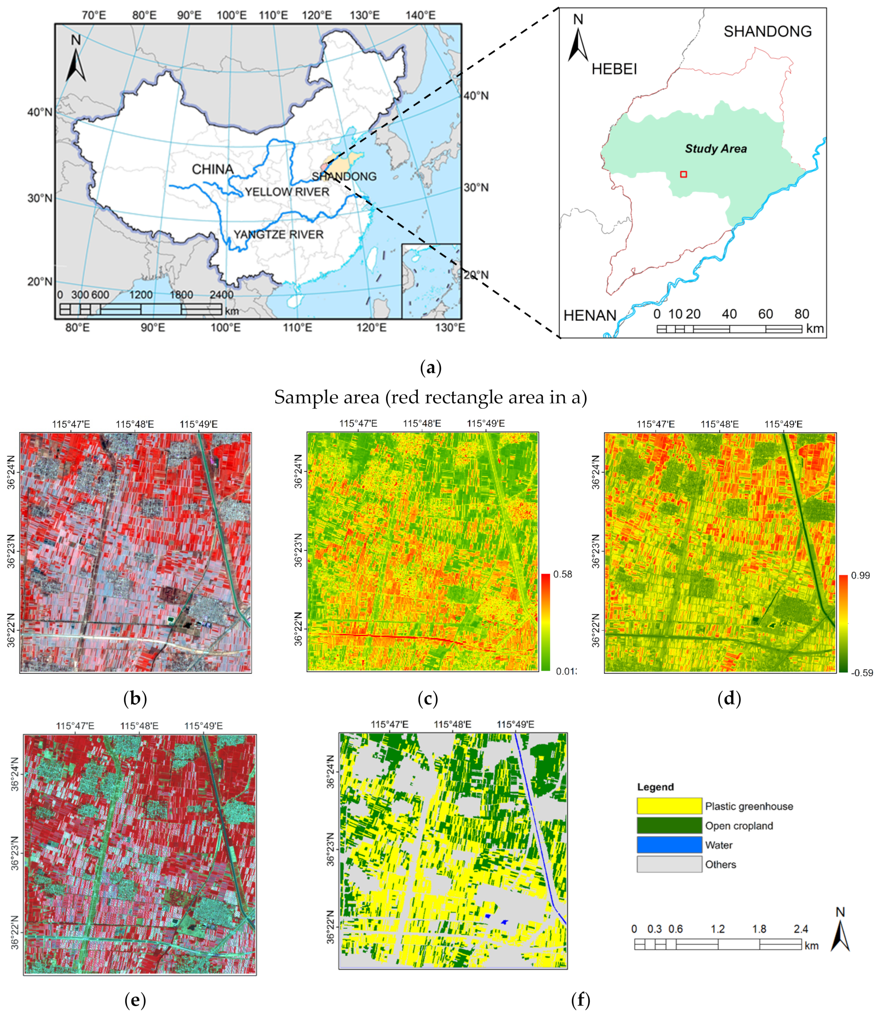
The Weishan Irrigation District is located in Shandong Province, China. It is the largest irrigation area at the lower Yellow River. Irrigation water for most of the cultivated land in this region is diverted from the Yellow River, and a large amount of water is required to alleviate the impact of drought every year. However, water use permits for the Yellow River to irrigate farmland are very expensive, and water diversion brings a large amount of sediment to the irrigation area too. It is necessary to map the regional planting areas, especially greenhouse facilities, and develop water conservation agriculture in the irrigation areas. This investigation was conducted in four counties within the irrigation district, including the Dongchangfu District, Guan County, Chipping County, and Dong’e County, which cover almost 4334 km2 (36°7’ N ~36°45’ N, 115°16’ E ~116°33’ E). In the Weishan irrigation district, more than 90% of PGs distributed in the study area. The study area and satellite data are shown in Figure 1.
2.2. Datasets and Pre-Processing
2.2.1. Sentinel-2 Multispectral Satellite Images (S2 MSI)
The Sentinel-2A satellite carried an innovative wide swath high-resolution multispectral imager with 13 spectral bands for a new perspective of monitoring land, forests, and crops. These working bands with three different geometric resolutions ranging from 10 to 60 m. Specifically, the High-Resolution Visible Images (Red, Green, Blue, and Near-Infrared bands) with 10 m GSD, and the red-edge, narrow near infrared, and shortwave infrared bands with 20 m GSD. With the launch of satellite Sentinel-2B, two sensors in orbit have significantly shortened the revisit time resulting in a five-day interval for Sentinel-2 images. Its superiority about spatio-temporal resolution provides adequate and high-quality data in areas, facilitating the broad application of the satellite images.
The S2 Level-1C images (S2 L1C) were top-of-atmosphere (TOA) reflectance products that were geometrically corrected (within one pixel) and radiation converted (absolute error of <5%). It provides spatio-temporal TOA reflectance products divided into 100 × 100 km2 UTM/WGS84 projected tiles. Atmospheric correction was performed using the Sen2cor plugin v2.3.1 to transform TOA reflectance into Bottom of Atmosphere (BOA) reflectance images (S2 L2A). Considering that our main task is object identification; thus, the Coastal aerosol, Water vapor, and Shortwave infrared cirrus bands of the S2 image were abnegated. In reference to the spatial scale of the High-Resolution Visible Images, fusing multispectral images to a higher GSD have a small damage on classification [42]. Hence, based on the Gram–Schmidt image fusion algorithm [43], newly red-edge and narrow near infrared bands that were registered to 10 m GSD rely on the High-Resolution Visible Images of S2 imagery.
In a word, 10 bands in the single-temporal S2 image are mainly considered in this research (1: Blue 458-523 nm; 2: Green, 543-578 nm; 3: Red, 650-680 nm; 4: Red-edge I (R-edge I), 698-713 nm; 5: Red-edge II (R-edge II), 733-748 nm; 6: Red-edge III (R-edge III), 773-793 nm; 7: Near infrared (NIR), 785-900 nm; 8: Narrow Near infrared (NNIR), 855-875 nm, 9: Shortwave infrared-1 (SWIR1), 1566-1651 nm; 10: Shortwave infrared-2 (SWIR2), 2100-2280 nm). S2 images from January to June 2019 in the study area were combined into dense S2 SITS data to support next experiments. Other two-temporal S2 images are aimed at detecting PGs of 2017 and 2021. The processed S2 SITS used in this research is shown in Table 1.
2.2.2. High-Resolution Image
GF-6 satellite (China) panchromatic and multispectral sensor (PMS) provided a panchromatic band with 2 m GSD, and four High-Resolution Visible Images with 8 m GSD. In this work, the PMS image derived samples for accuracy assessment. We processed the image with orthographic correction and image fusion to acquire a VHR image with 2 m GSD. Later, the VHR image was registered with S2 images to ensure that S2 and GF-6 images had the same coordinate system.
2.2.3. Survey Data
The field-level photos with Global Navigation Satellite System (GNSS) positional information provided locations, which are not as accurate as professional surveying equipment, but are simple and feasible for collecting sample data in agriculture [44]. Several brief field campaigns were conducted in January, June, and July 2019 to gather geofield photos of open-cropland, PGs, and PMF. These field-level photos were aimed at assisting artificial interpretation of VHR images and establishing a sample database. As shown in Table 2, numerous samples were selected to establish the database. The whole study area’s sample data were split randomly into training and test sets, approximately following the ratio of 60%:40%. In addition, two sets should keep class distributions in all groups that are similar and independent from each other. Finally, the training set and test sets were to train an individual classifier and optimize the model, respectively.
3. Methodology
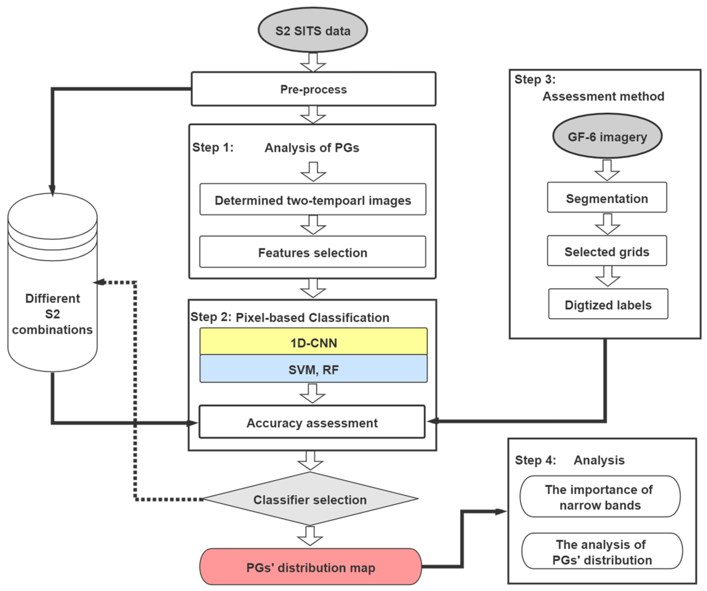
This research is mainly composed of four parts. In Figure 2, the middle section of the main flow describes the PGs mapping technique with two-temporal S2 images. With dense S2 SITS data, we searched PG’s characteristics and determined the two periods S2 images and vital features (Step1). Then, a 1D-CNN classifier was adopted to deeply mine the linear arrangement’s features, thereby achieving PG detection. To verify the proposed method’s superiority, we conducted comparative experiments for pixel-based classifiers (1D-CNN, SVM, and RF) simultaneously (Step 2). Assessment reports of comparisons desperately need requisite and objective assessment methods. Therefore, Step 3 of the framework describes the production of labels. On the left side of the framework, PG maps using single-temporal and multi-temporal S2 data were compared to verify this study’s reliability. In addition, we explored the importance of the narrow bands with a comparative experiment. On the basis of achieved maps, we undertake a meaningful investigation of the PGs’ spatial distribution. The framework of the scheme is shown in Figure 2.
3.1. Analysis of PGs
3.1.1. Spectral Characteristics of PGs
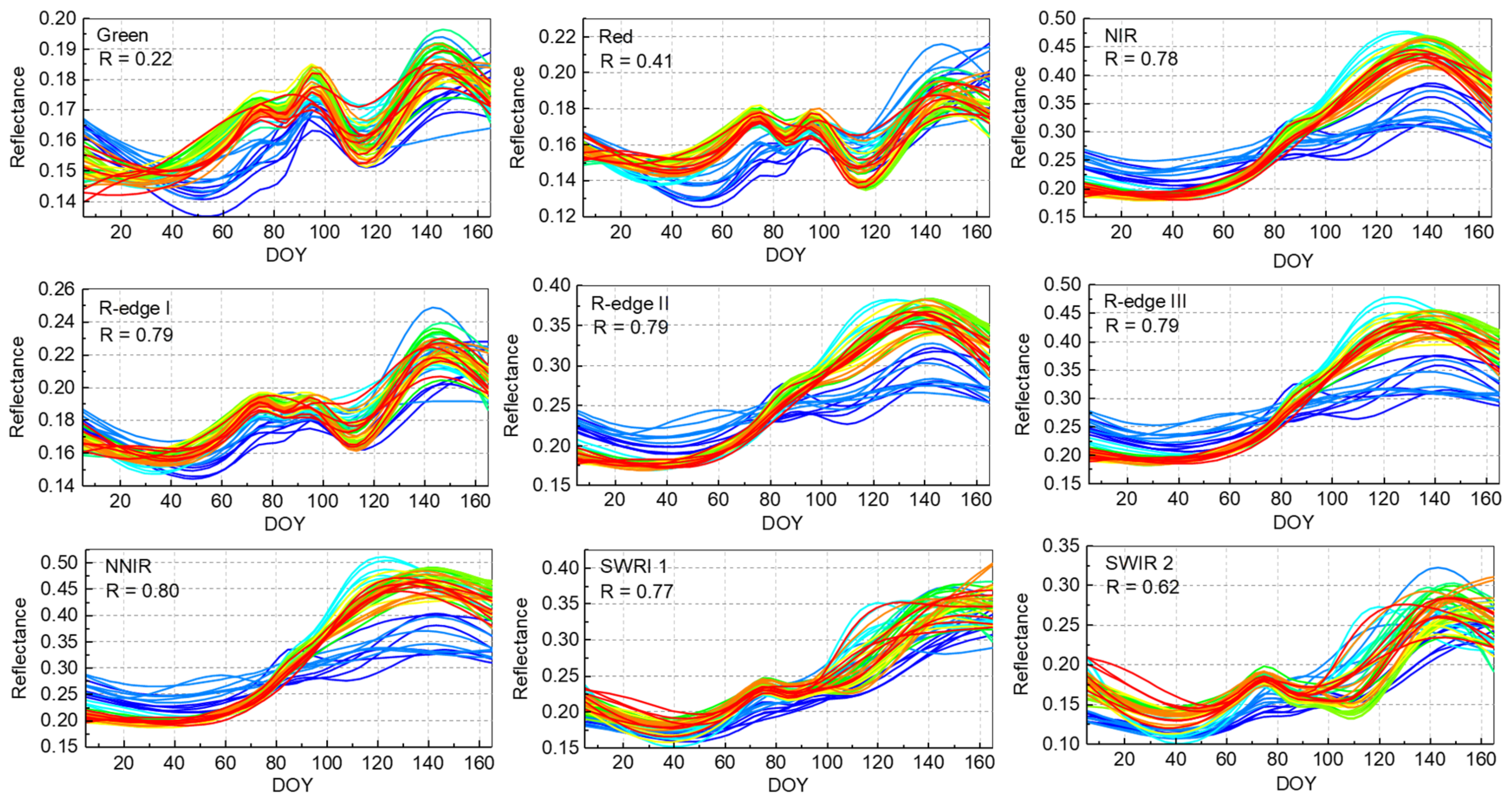
Spectrum analysis is necessary for object recognition and information interpretation [45]. The spectrum of 50 representative PG fields (total 1156 pixels) of different materials and shapes were obtained from S2 SITS. First, the acquisition date of S2 SITS was converted to the day of year (DOY). Then, we obtained average reflectance value for each field to simplify the following analysis. Finally, the correlation between the time variables (DOY) and the PG’s reflectance in each band was analyzed in the Statistical Package for the Social Sciences software. The changes in different bands of 50 PGs were also visualized (the blue wavelength is not shown because it has no obvious pattern).
From Figure 3, the PG’s reflectance at 705–865 nm was positively correlated with time. Specifically, the reflectance at 865 nm and 740 nm was most remarkable, with an average determination coefficient (R) of 0.80 and 0.79, respectively. The results show that the reflectance of PGs in the red-edge and near-infrared bands increased in the vegetative cycle of inner crops. It indicates that the crop growth characteristics were also revealed in remote sensing images, even though the crops were covered by plastic film. The seasonal characteristics are innovative features to detect PGs. Meanwhile, the R-edge I~III, NIR, and NNIR band reflectance with the most regular changes announced that S2 images provided more additional information than Landsat imagery. With these remarkable features, detecting PGs with fewer S2 images is reasonable.
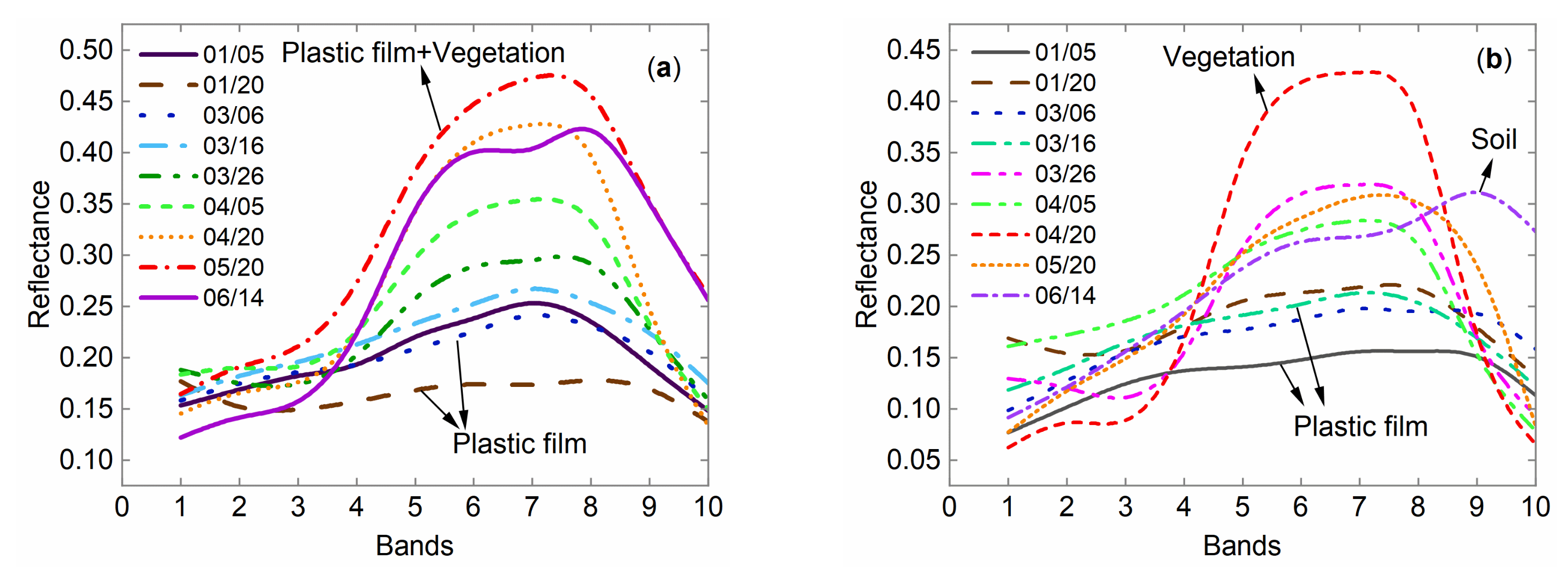
To determine the crucial period images, the unique spectral response with the time of PGs and PMF were also revealed in Figure 4a,b. In March, the PG spectrum is untouched by the crops in a PG. However, in May, the reflectance is affected by both the plastic film and the crops inside. As a result, the R-edge I~III, NIR, and NNIR bands increased and reached the peak in May, then declined over time in the crop vegetation cycle. In addition, the reflectance of PMF reached the maximum value in April and remained relatively high in May. In agriculture, plastic film is regarded as a protective screen for crops in cold waves. When the temperature rises, the plastic film is removed. Thus, in April, PMF reflects the characteristics of vegetation entirely during the vigorous growth period.
We adopt a strategy that combines two crucial period S2 images in which the most obvious difference of the PG spectrum embodied to form a special spectral curve. Figure 4c demonstrated that two-temporal stacked S2 imagery (March 6 and May 20). This unique curve has the double advantage of both the characteristics of the plastic film and the interior vegetation, increasing the weight of extracting PGs. From Figure 4d, NDVI also plays an important role in differentiating open-farmland and plastic-covered farmland. The NDVI of open-farmland was significantly higher than that of plastic-covered farmland. From January to June, the NDVI of PGs that contained crops increased gradually. However, the PMF showed a significant increase in late April and early May.
The aforementioned analysis for several typical features reinforces that dense S2 SITS data detected PGs and even PMF easily. Note that the S2 SITS data are complicated and hysteretic to support the PG fast-monitoring system. The combinations of two crucial periods’ S2 images are effective to reduce the complexity of project. Therefore, in this research, the first attempt about detecting PGs relied on the aforementioned two-temporal S2 imagery.
3.1.2. Building Features to Highlight PGs
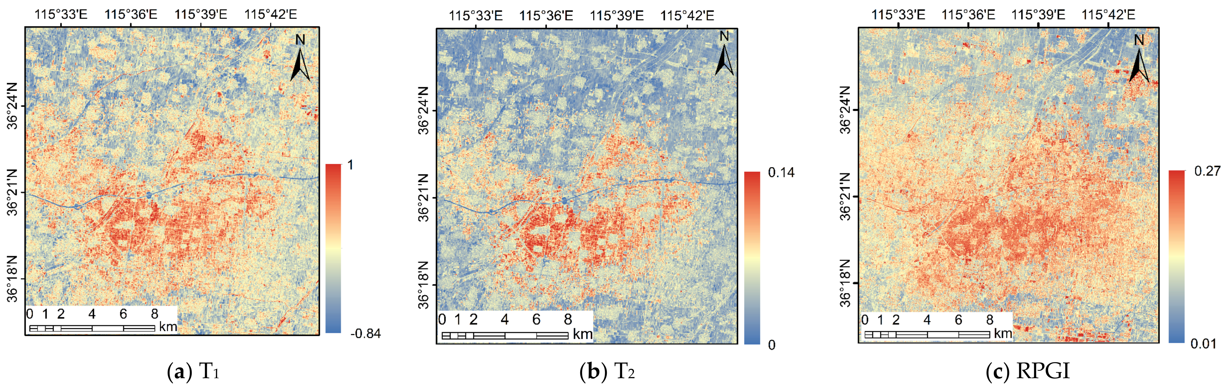
The analysis provides some enlightenment to a certain degree. The reflectance of PGs in R-edge I~III and NNIR bands maintained a low value in March, reaching the peak in May. Note that the NNIR band revealed the most regular changes (i.e., its determination coefficients were most remarkable). In reference to the establishment of the normalized differential vegetation index (NDVI), the enhanced feature of PGs (T1) was calculated by the difference in reflectivity of different periods’ S2 images. Specifically, our idea is to quantitatively describe the reflectance difference of NNIR band in March and May, and scale the difference between 0 and 1. According to the aforementioned analytical knowledge, PG’s reflectance difference in March and May is obvious. Thus, its value is higher than other surface objects. In addition, T2, that is, the second calculated feature, is the combination of T1 and RPGI. The target of T2 was to bring the seasonal characteristics of PGs to the RPGI for obtaining a new prominent feature:
where is the NNIR band of the 20 May S2 image, and is the NNIR band of the 6 March S2 image. In particular, the red-edge bands also met the requirements for the calculation of the combinations.
3.1.3. Features Participated in the Classification Process
The classification features used in this work (Table 3) were retrieved from two-temporal S2 images. First, a distinct spectral sequence of two-temporal S2 images is a pivotal identification code for PGs. Next, the PG enhanced features were selected to improve mapping results. On the one hand, the features representing the seasonal characteristics of PGs, such as T1 and T2, were well organized. On the other hand, some commonly used PGs indexes (proposed by previous research) were also utilized. The features were organized as shown in Table 3.
3.2. Image Classification Methods
To obtain the PGs’ spatial distribution based on two-temporal S2 imagery, a strategic approach is needed to represent the spectral variation and mine in-depth information. The pixel-based 1D-CNN algorithm is a neural network specially designed to process spectrum time series data and has achieved excellent performance [47]. By employing a multi-layer network to mine and extract high-dimensional data features, deep learning 1D-CNN can automatically learn the relationships hidden inside the data [48].
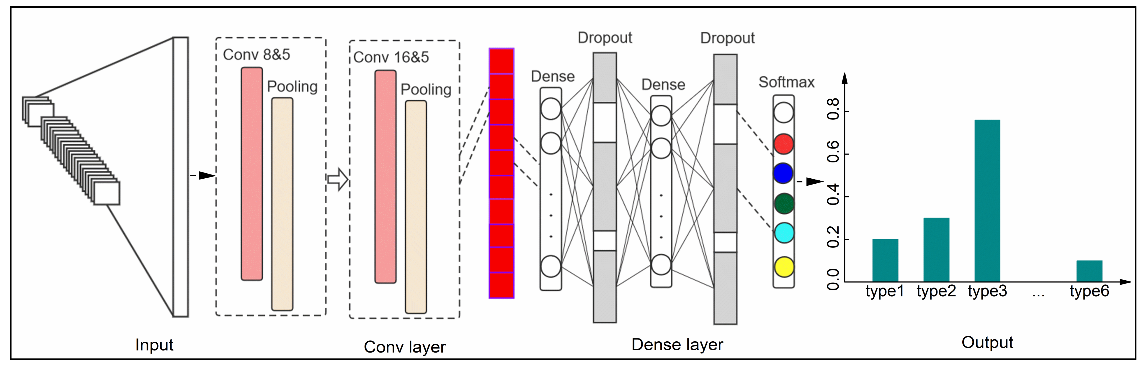
A complete 1D-CNN model comprises four parts: input, output, convolution layer (Conv layer), and dense connection layer (Dense layer). First, the input part throws the spectral and index features into the network model. The convolution part consists of two convolution layers and two pooling layers. Using these convolution layers, the subtle features of sequence data are amplified and captured intelligently. The Conv layer captures the changes spectral by traversing the continuous curve deeply. This is indispensable and crucial to realize our theory of detecting PGs with two-temporal S2 images. In this study, we initially applied eight convolution kernels of size 5 to extract the features. Then, in the second convolution layer, we applied 16 kernels of the same size as that previous step to mine the components further. In addition, the two pooling layers aimed to refine features and reduce redundant information. The dense layer consists of a flattening layer, dense layer, and dropout layer. The function of the flattening layer is that it puts the learned multi-dimensional features as a linear arrangement to support the next work. The dense layers adopt feedforward transmission mechanism to map the distributed features to the sample space, whereas the dropout layer mainly prevents overfitting. Finally, we convert the output of the last layer into the probability of a certain class through a series of operations. The structure of 1D-CNN is shown in Figure 5.
3.3. Assessment Methods
The confusion matrix analysis is a commonly used method to assess classification results. Typically, two main methods are commonly used. The first is confusion matrix analysis using real areas of interest in the classified images. This method is subject to much human interference. Additionally, the selected area of interest lacks an adequate representation and cannot accurately assess the classification results in all respects. The second method is confusion matrix analysis using ground truth images. The core of the second assessment method is the production of ground truth images. Unfortunately, it is almost impossible to obtain vectored labels for a large-scale area on time. The assessment reports absolutely rely on ground truth labels only under ideal conditions; in practice, they are far behind real-world conditions.
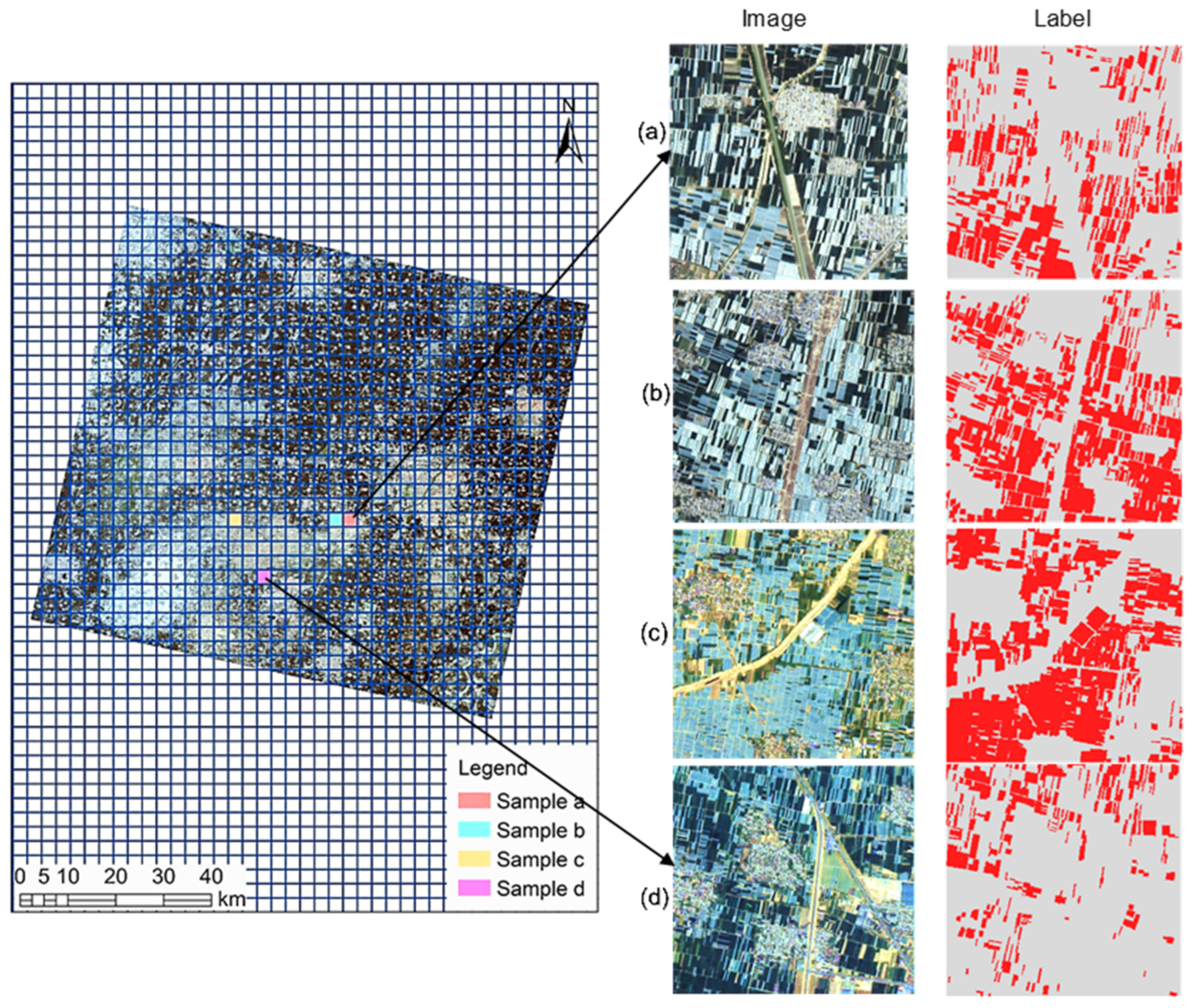
Thus, we adopted a new method that combines the advantages of two conventional evaluation methods to cope with the binary classification in PG and non-PG classes. As shown in Figure 6, we divided the GF-6 image of the study area into a 3 × 3 km grid. Then, we randomly selected "grids image" to represent the PGs’ distribution in the study area on a divided checkerboard. We artificially interpreted every grid image (manually drew labels) to obtain the ground truth labels and resampled to 10 m GSD. Ultimately, the binary classification accuracies (PGs or non-PGs) were assessed quantitatively by the confusion matrix based on manually drawn labels (i.e., the assessment results from the error matrix of the sub-image classification maps and labels). To guarantee the evaluation objectively and comprehensively, four samples with two grids with a dense PG distribution and two with a sparse distribution were selected to evaluate the corresponding classification results synthetically. The main reason was to provide a realistic representation of PG distribution in the study area and ensure the assessment was convective. Meanwhile, the work of various sample productions was reduced.
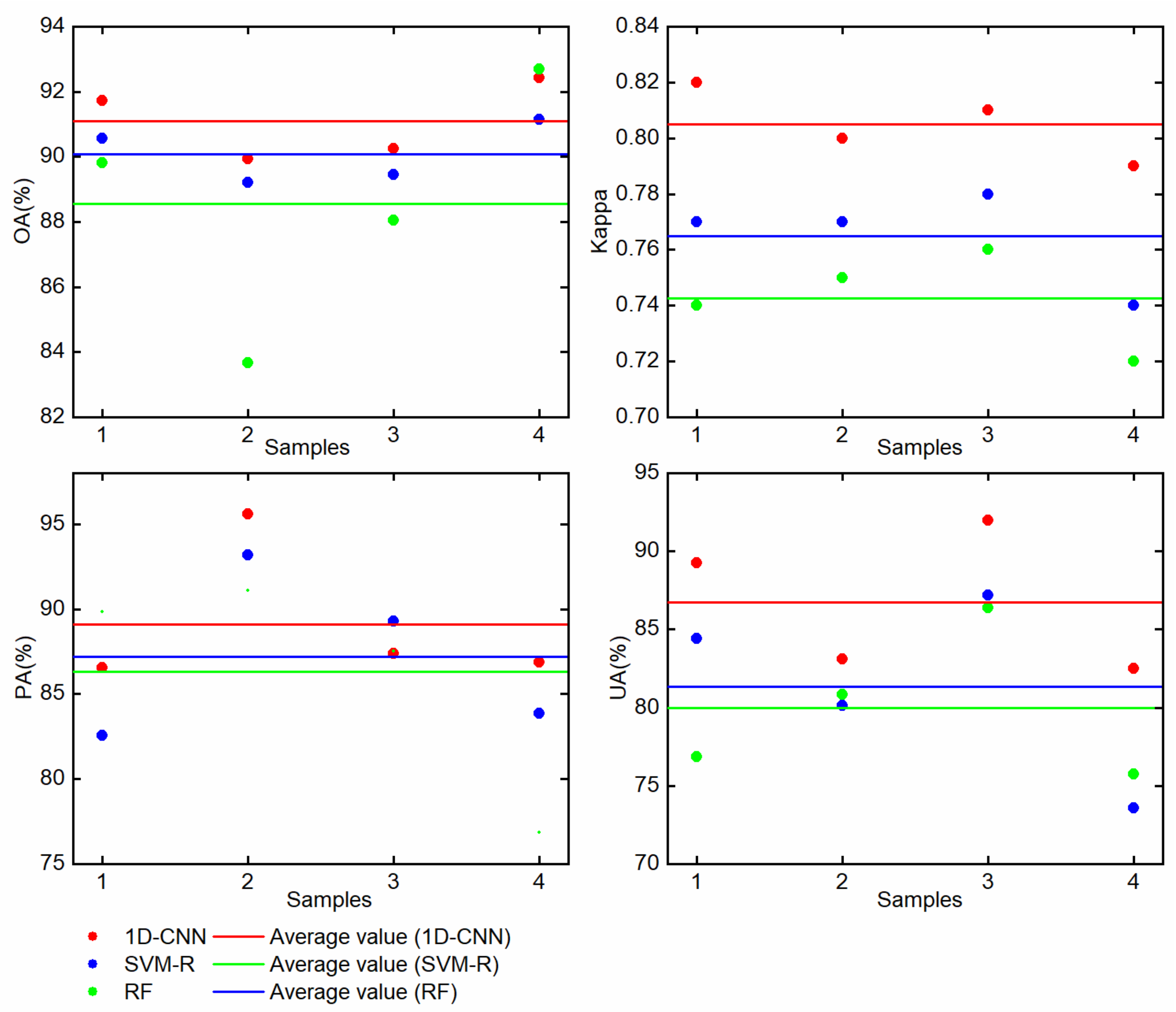
In this work, we used four indices to evaluate the PG detecting results: overall accuracy (OA), kappa coefficient (kappa), producer accuracy (PA), and user accuracy (UA). The aforementioned method offers a reliable assessment which matches a 3 × 3 km classification map with the same real labels. Moreover, the final assessment results were an average of the assessment results of the four grids.
4. Results
4.1. PGs’ Spatial Distribution Map
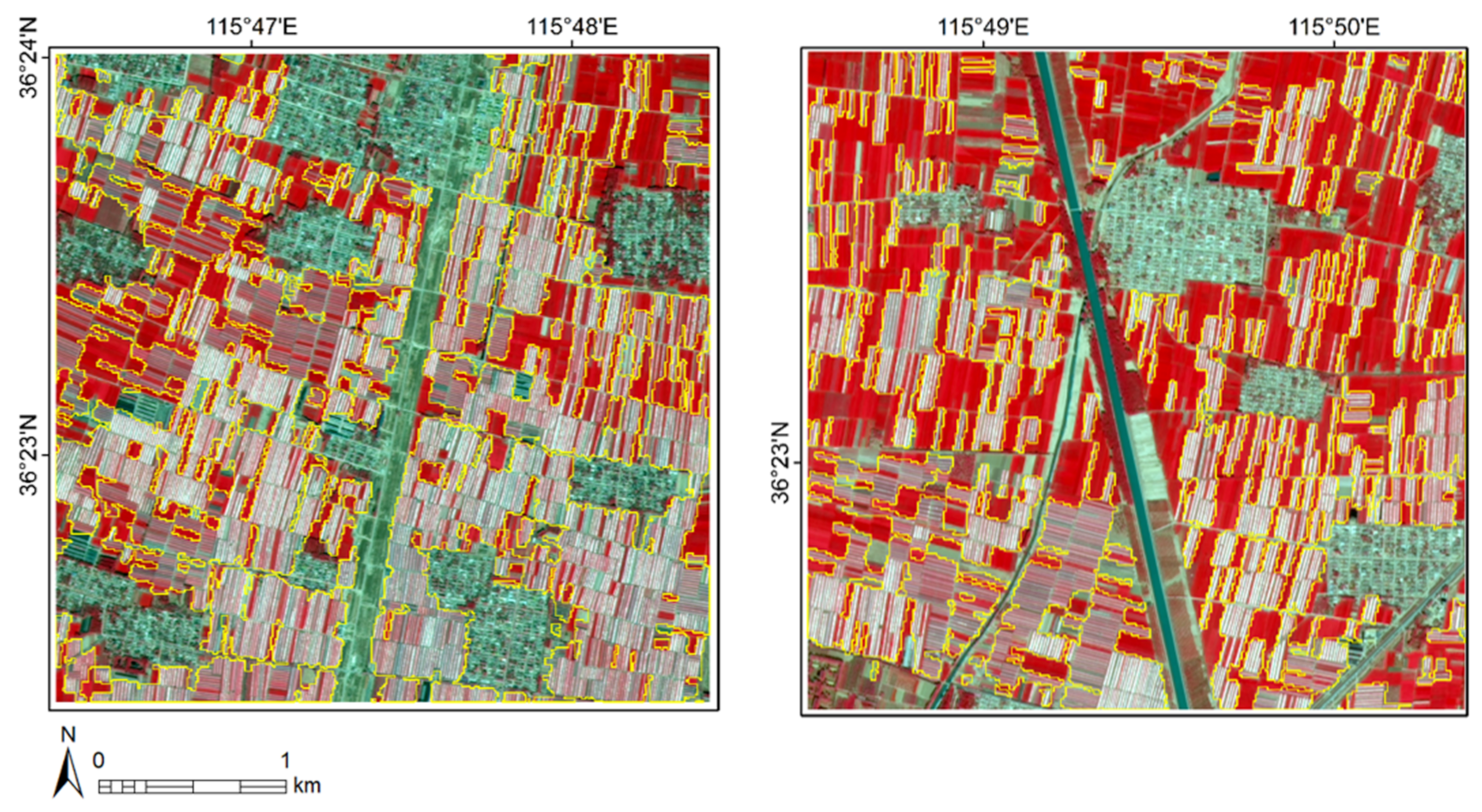
Feature selection for the two aforementioned temporal S2 combinations provided the significant spectral difference of the PGs. The PGs’ spatial distributions from per-pixel classifier matched the natural surface and field survey results of the same area. From Figure 7, the 1D-CNN approach drew the accurate boundaries of PGs of different materials and shapes. Additionally, the results displayed in the visible VHR image (GF-6) of a typical region showed that dense and scattered PGs were also extracted accurately. As another implication, the PG maps using 1D-CNN and S2 imagery maintained fine-grained mapping while applying to a large scope.
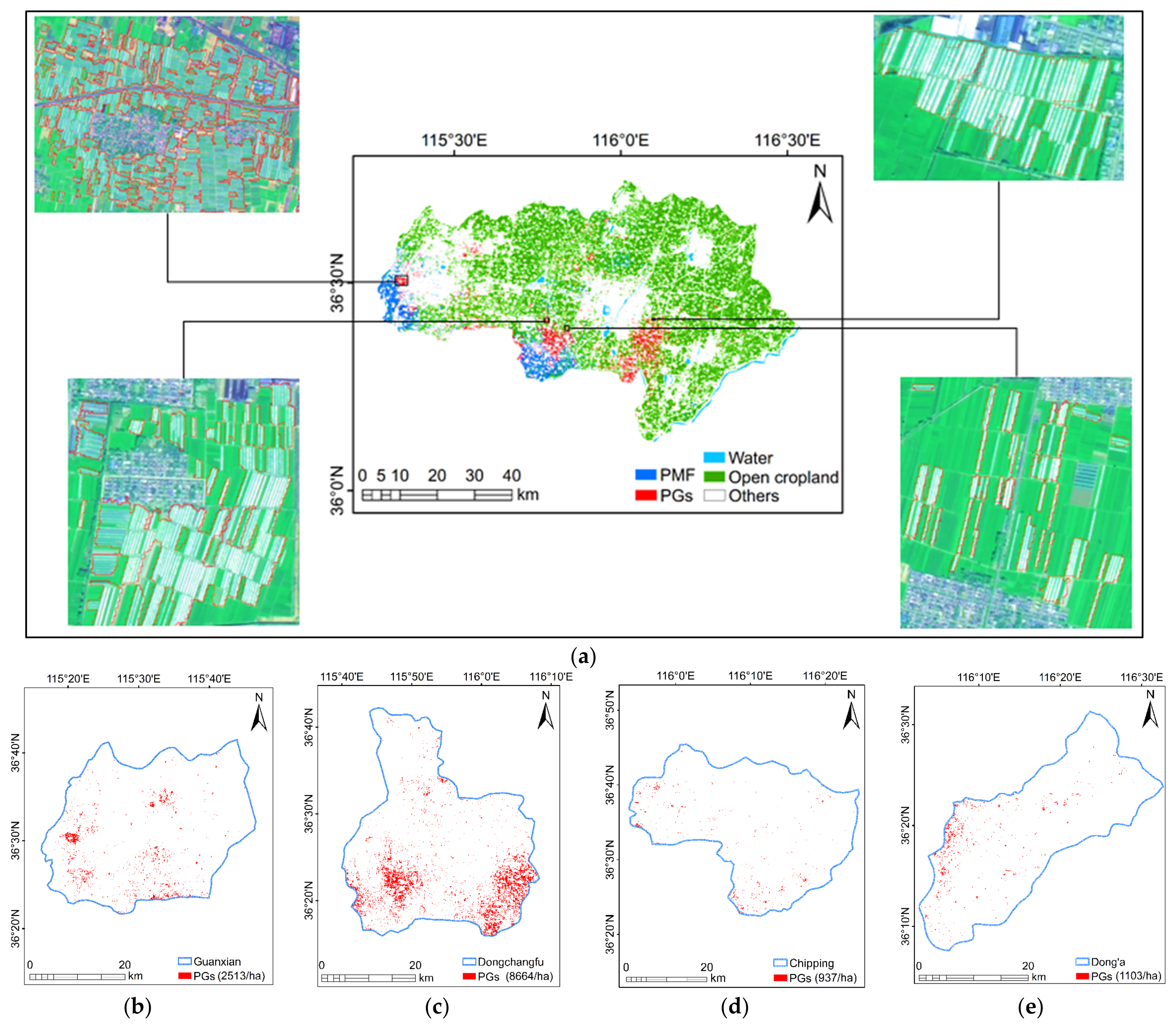
In addition, the regional PG distribution was also obtained efficiently by the proposed method (Figure 8). This project provided the thematic maps and necessary statistical data (Dongchangfu District, 8664 ha; Guan County, 2513 ha; Chipping County, 937 ha; and Dong’e County, 1103 ha), which is valuable for local agricultural management and policy implementation. Under the fewer limitations of the data source and computation, the two-temporal images increased the feasibility of practical applications. In addition, the crucial data were not limited to the combination of March and May images. Instead, they principally used the obvious red-edge and near-infrared changes of the PGs in the S-2 embodiments.
4.2. Accuracy Assessment
4.2.1. Accuracy Assessment of Different Classifiers
For pixel-based classifiers, comparative results are indispensable for accounting for the advancements of the 1D-CNN method. Therefore, in this experiment, we carried out three commonly used pixel-based classifiers 1D-CNN, SVM-R (SVM method with RBF kernel), and RF to detect PGs. The gamma and the penalty coefficient of SVM-R were 0.043 and 100, respectively. In addition, the estimator and depth of the RF model were set to 200, and 8 was an appropriate choice. Specifically, all the optimal parameters of SVM and RF shall be explored according to the training samples. Ultimately, in Figure 9, various assessment reports were produced by four acknowledged indicators to provide discernible information about three per-pixel classifiers.
The SVM and RF classifiers both achieved favorable PG maps with an average kappa coefficient of 0.77 and 0.75, respectively. These are consistent with real labels from VHR images, and imply that extracted PGs with two-temporal S2 images are workable. The RF results had an average PA of 86.32% and UA of 79.96%. The results of SVM-R classifier were better than those of RF, particularly in favored indicators of users that kappa and UA improved by 0.02 and 1.38%. From the auxiliary line of Figure 9, the 1D-CNN classifier gets a promotion compared with SVM and RF, and various assessment indicators showed that OA, kappa, PA, and PA increased minimally by 0.67%, 0.04, 4.36%, and 5.38%, respectively. This classifier provided a map with an average kappa coefficient of 0.81, derived the optimal PG maps from all sides. Impressively, the Kappa and UA of the ideal maps improved significantly.
4.2.2. Accuracy Assessment of Different Combinations
In the foregoing assessment, the 1D-CNN classifier achieved an optimum result. Therefore, the PG maps of different combinations were explored with a 1D-CNN classifier. From Table 4, the single S2 data failed to obtain the desired results, with an average kappa coefficient of 0.69, PA of 74.55%, and UA of 85.70%. Multi-spectral S2 imagery with a few bands was insufficient and limited for high-precision PG mapping. Depending on the time continuity and sufficient spectrum, dense S2 SITS data were excellent for detailed crop recognition, PGs, PMF, crop growth state monitoring, and growth cycle monitoring. However, no optimization of feature selection or selecting special features to enhance a type, the classification process incurred data redundancy and a locally optimal solution. In Table 4, the PG maps with a dense distribution (sample (b)) failed to meet expectations. In the convolution process, the 1D-CNN model so overlearned the features required to map PGs as accurately that the PG map lost the rational shape of farmland. Additionally, a similar problem occurred for sample (b).
Compared with dense S2 SITS, two-temporal crucial images were competent for detecting PGs and even have better results. First, the PG spectrum in two-temporal stacked imagery was gradually raised because of the effects of crops on later-temporal images. Moreover, the changes of other objects, such as PMF, cropland, roads, built-up, and blue factories, were entirely different. Thus, the 1D-CNN model effectively detects PGs by traversing curves and extracting features. Then, the quantitative features of PGs promoted accurate recognition. The last can be summarized as two-temporal crucial images vastly reduce data redundancy. The dense S2 SITS data are often shadowed by clouds, resulting in the absence of satellite images. For large-scale projects, the massive amount of computation is also a burden, which limits its practical application. Conversely, two-temporal combinations were not limited to the combination of images in March and May. Instead, it just considered the spectral differences theory of PGs. Small restrictions, less data computation, and simple methods are conducive to the rapid establishment of a regional PG monitoring system.
4.3. Analysis of PGs’ Distribution
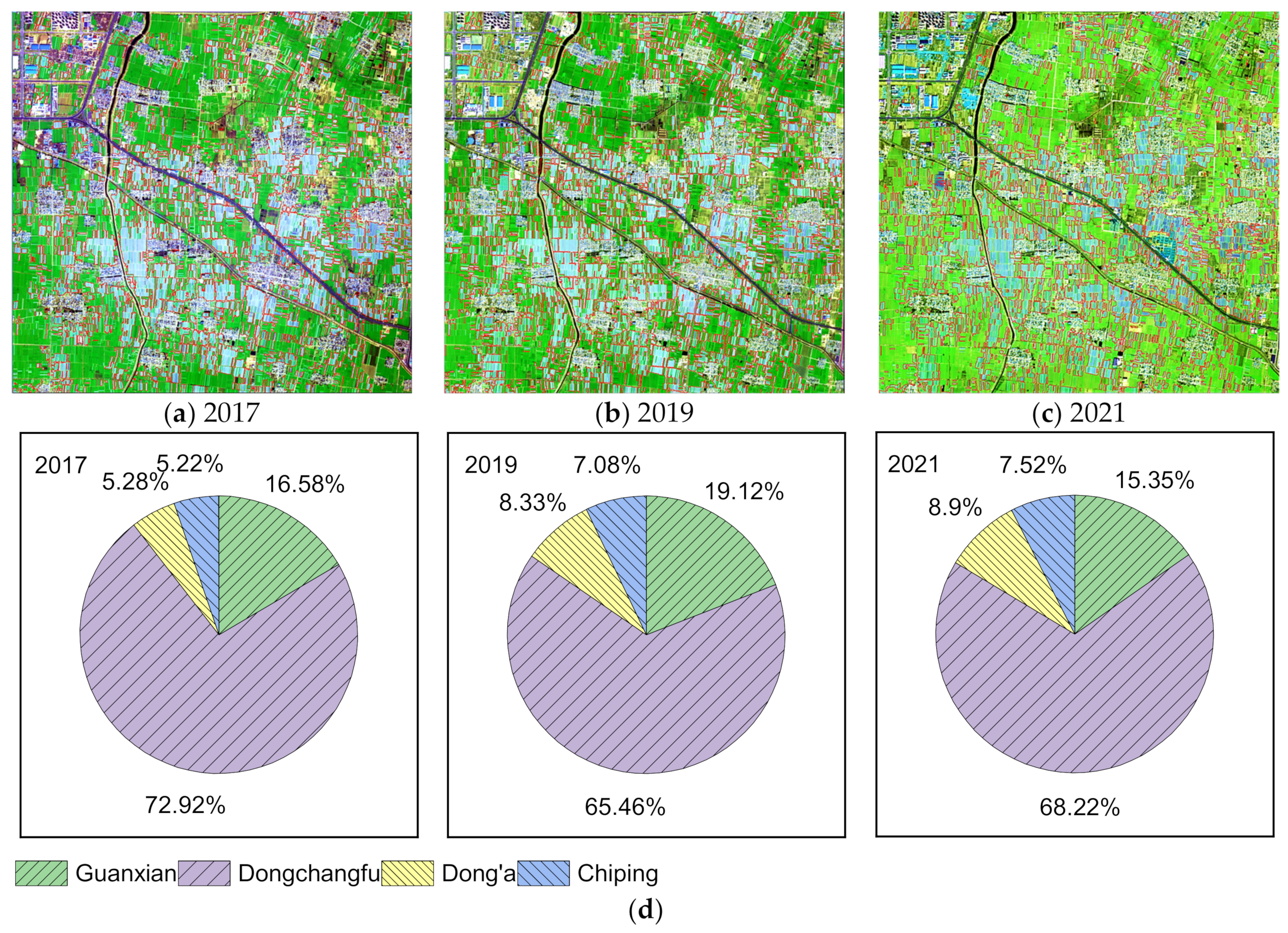
According to the suggested approach, the PGs’ spatial distribution of 2017, 2019, and 2021 were obtained. On one hand, these results verified applicability of this method further. On the other hand, it provided basic data for analyzing the dynamic change of regional PGs. From Figure 10a–c, the PG distribution of different years showed that detecting PGs with two-temporal S2 images and 1D-CNN is accurate and efficient. It proved that this scheme did not provide a reliable result accidentally but had good practicality. PGs’ statistics of years in study area were 13681 ha in 2017, 13235 ha in 2019, and 11232 ha in 2021, respectively. As shown in Figure 10d, the total area of PGs decreased, but the area is increasing in Dong’e and Chiping. On the other side, the area in Dongchangfu and Guan County did not show a regular trend of increase or decrease but was in a dynamic change mainly affected by the vegetable economy in recent years.
5. Discussion
5.1. Importance of the Narrow Bands of S2 for PG Mapping
The narrow bands (R-edge I~III and NNIR bands) are typical features of S2 imagery. However, previous studies of PGs had few considerations of narrow band changes and their function. The two PG enhanced features T1 and T2, which were created with two-temporal NNIR band difference, were sensitive to the PGs. From Figure 11, RPGI may reveal more details, but the RPGI threshold is not applicable to S2 imagery with no normalized difference building index. T1 and T2 quantitatively highlighted PGs and distinguished them from open cropland, built-up, road, and water, although they also contained some noise. To apply the suggested features to S2 images, it is extremely important to identify the lower and upper thresholds. After frequently repeated classification threshold experiments, it was found that a T1 between 0.025 and 0.040 had a high separability of PGs from other objects. According to experiments, a T2 between 0.23 and 0.47 performed better for PG detecting. It is difficult to detect PGs accurately by T1 and T2 thresholds, but their essential features deserve particular attention in the classification process.
The RF algorithm not only acted as a classifier but also served as a variable importance estimation and feature selection method based on a decision tree [49]. In this study, we closely measured the importance of narrow band information for PG mapping using this method. From Figure 12, all bands of two-temporal S2 images played certain roles, with marginal differences.
With the spectrum of two-temporal images, the Red, R-edge III, NIR, and SWIR bands have a higher contribution rate in distinguishing open cropland, PGs, PMF, unused land, and construction. However, for well-organized two-temporal combinations, the R-edge and SWIR bands play a predominant role. The main reason is that R-edge bands of S2 imagery are sensitive for vegetation, which are capable of detecting crops, PGs, and PMF. And the enhanced PG features have an outstanding performance. T1 and T2 have contributed up to 9.4% of PG mapping, and its performance is as robust as that of widely recognized RPGI and PMLI. Note that the importance of the information related to narrow bands accounted for 39.11% of the total, indicating that they were efficient for fine mapping.
Two contrastive PGs maps, produced with and without narrow bands, were to describe the specific effect of narrow bands. As shown in Table 5, the information related to narrow bands improved the PG detection ability to a certain extent. The four indicators OA, kappa, PA, and UA increased by 4%, 0.08, 2.96%, and 2.21%, respectively. The experiment results show that PG mapping accuracy was clearly improved by using the narrow bands.
5.2. Discussion of the Data and Classification Methods
Regarding PG mapping with the VHR image, the object-based image analysis (OBIA) is one of the mainstream methods, except the pixel-based method. The OBIA approach minimized noise and maintained the shape of farmland, thereby resulting in the classification map rationale. In that case, Aguilar et al. [7,16,18,19,25], Novelli et al. [33], and Pala et al. [4] held the lead (Table 6). These researchers devoted to high-precision mapping of PGs, PMF, and horticultural crops under plastic coverings using OBIA. In China, Zhao et al. [20] obtained high-precision maps with VHR images and the OBIA approach, but only in the countywide scope. To obtain the PG distribution and quantitative statistics, VHR images are accurate but more costly applied to large areas. Aguilar et al. [26] and Novelli et al. [33] attempted to extend PG’s segmentation results from VHR images to multi-spectral imagery (Landsat 8 or Sentinel-2 imagery), which is effective for combining rich textures with an extra spectrum. This is an excellent choice for producing time series PG maps that rely on free satellite images. However, these studies were all restricted to the width of VHR images.
Landsat images have several advantages, such as open access, continuity of the time series, and the mapping of PGs and PMF on a large scale. For Landsat images, Ji et al. [50] and Wu et al. [51] used the OBIA approach for PG mapping. They applied it to extracting PGs with a dense distribution, but there was still a sustainable challenge for scattered PGs. In the OBIA approach, three critical issues need to be emphasized. First, the segments should represent the shape of real individual PGs. Second, OBIA emphasizes using textures and a spectrum of imagery comprehensively [52]. It seems that the OBIA approach is more suited to high spatial resolution images with rich textures. Finally, the object-based classifier uses image objects rather than pixels. Thus, adequate field samples and investigations are needed for training the classification rule.
PG monitoring with wide-covered and medium resolution Landsat images and the per-pixel classifier were commonly used. Yang et al. [22] developed an index for direct PG mapping. Hasituya et al. [23,27] and Lu et al. [28] monitored PMF with a pixel-based classifier on a large scale. This research was associated with per-pixel techniques and large-scale mapping. In China, PGs are widespread and not concentrated, as in Spain. A PG-monitored scheme is typically implemented in an irrigated district, prefecture, or even province. The principles of the OBIA suggest that it is a segmentation process for big data with extensive calculations [53,54]. This method increases the complexity of practical applications in regions.
Regarding the data source, it is difficult for Landsat images—with few bands and medium temporal resolution—to monitor crop growth in a PG and reflect the subtle changes of PGs in detail. Due to the adverse effects of mixed pixels, PG mapping with higher spatial precision remains a sustainable challenge. The dense S2 SITS data detected the reflectance changes over time by using the red-edge and near-infrared bands, proving a novel approach to analyze the seasonal characteristics of PGs. The dense S2 SITS data changes indicated the effects on the PG’s reflectance caused by crop growth. These conditions all suggest that fine-grained S2 SITS data are highly applicable for both PGs and horticultural crops inside. To reduce computational cost, two-temporal S2 images could be selected from S2 SITS representing obvious seasonal spectral difference. Benefiting from the convolution layer, the 1D-CNN classifier focused on amplifying the spectral changes and extracting subtle features. The visualization of the representative region showed that this classifier had a prominent role in PG mapping. In addition, the 1D-CNN classifier performed better than traditional pixel-based classifiers, such as SVM and RF.
Compared with the current methods of PG mapping (Table 6), this research provided a more practical framework and obtained a fine and large-scale PG map, which had less data calculations, efficient implementation, and fewer data constraints. Incidentally, the spatio-temporal resolution of S2 imagery is higher than that of Landsat imagery. This promises the release of free thematic maps of PGs on large areas with a higher spatial resolution. To summarize, both OBIA and 1D-CNN have unique strengths and application scenarios. The per-pixel technique of 1D-CNN is more automated and convenient than OBIA for PG monitoring systems in a large area. However, a limitation of the 1D-CNN method is that the classified maps of the PGs contain pepper noise. As cloud computing evolves and further research is conducted, a classification method that combines OBIA and 1D-CNN should be investigated [55]. Advanced deep learning models that fuse spatial and spectral information may promote PG mapping using S2 images [56].
6. Conclusions
In this paper, we evaluated S2 SITS images (especially in two critical periods) to determine the suitability for mapping PGs in Weishan Irrigation, Shandong Province, China. Then, a 1D-CNN classifier was proposed to cater for two-temporal images. In addition, we tested the performance of the 1D-CNN classifier and different combinations of features. Finally, the contribution of information related to narrow bands for monitoring PGs were discussed. The detailed conclusions are as follows:
- The analysis of dense S2 SITS indicated that the PG’s reflectance was not changeless but continuously changed in crop growing seasons. The reflectance of the red-edge and near-infrared bands increased gradually over time and reached the maximum in late May. Hence, two critical periods’ images reflecting that an enormous reflectance difference was suitable for mapping PGs.
- When detecting PGs with two-temporal S2 images, 1D-CNN learned more detailed PG features by mining slight increases and decreases in the spectrum. Thus, the 1D-CNN classifier had a promotion compared with SVM and RF, which derived the best mapping results from all sides. The assessment indicators OA, kappa, PA, and PA increased by approximately 6%, 0.04, 3%, and 4%, respectively.
- The contrastive experiment with different temporal combinations showed that two critical period images were adequate and sufficient for PG mapping. The classified maps highly matched the real labels produced by GF-6, intuitively demonstrating the accurate results.
- In two-temporal S2 images, the variation of the narrow bands improved the PG mapping accuracy. The four indicators OA, kappa, PA, and UA of the final maps increased by 4%, 0.08, 2.96%, and 2.21%, respectively. The proposed combinations (T1 and T2) of narrow bands were also essential and unique to reflect the PGs’ spatial distribution.
Author Contributions
Methodology, H.S.; Formal analysis, H.S., L.W., Z.Z.; Data curation, H.S., R.L.; Funding acquisition, L.W.; Project administration, L.W., B.Z. All authors have read and agreed to the published version of the manuscript.
Funding
This research was funded by the National Key Research and Development Program of China (No. 2018YFC0407703).
Data Availability Statement
Dense Sentinel-2 Satellite Image Time Series data are available free of charge from the ESA Data Hub. Furthermore, the China High Resolution Data Application Center provided fine 2 m/8 m GSD multi-spectral images. Upon a reasonable request, the gainable remote sensing data and the source codes that support the findings of this research are available from the first author (H.S.).
Acknowledgments
We would like to thank the anonymous reviewers for their patient guidance and constructive comments. Moreover, we are grateful to the China High Resolution Data Application Center provided VHR image for free.
Conflicts of Interest
The authors declare no conflict of interest.
References
- Benz, U.C.; Hofmann, P.; Willhauck, G.; Lingenfelder, I.; Heynen, M. Multi-resolution, object-oriented fuzzy analysis of remote sensing data for GIS-ready information. ISPRS J. Photogramm. Remote Sens. 2011, 58, 239–258. [Google Scholar] [CrossRef]
- Bai, L.T.; Hai, J.B.; Han, Q.F.; Jia, Z.K. Effects of mulching with different kinds of plastic film on growth and water use efficiency of winter wheat in Weibei Highland. Agric. Res. Arid Areas 2010, 28, 135–139. [Google Scholar] [CrossRef]
- Jing, L.; Gengxing, Z.; Tao, L.; Yude, Y. Study on Technique of Extracting Greenhouse Vegetable Information from Landsat TM Image. J. Soil Water Conserv. 2004, 18, 126–129. [Google Scholar]
- Pala, E.; Taşdemir, K. Fast extraction of plastic greenhouses using Worldview-2 images. In Proceedings of the 2016 IEEE International Geoscience and Remote Sensing Symposium (IGARSS), Beijing, China, 10–15 July 2016. [Google Scholar]
- Jensen, M.H.; Malter, A.J. Protected Agriculture: A Global Review; World Bank Publications: Washington, DC, USA, 1995; Volume 253. [Google Scholar]
- Levin, N.; Lugassi, R.; Ramon, U.; Braun, O.; Ben-Dor, E. Remote sensing as a tool for monitoring plasticulture in agricultural landscapes. Int. J. Remote Sens. 2007, 28, 183–202. [Google Scholar] [CrossRef]
- Jiménez-Lao, R.; Aguilar, F.; Nemmaoui, A.; Aguilar, M. Remote Sensing of Agricultural Greenhouses and Plastic-Mulched Farmland: An Analysis of Worldwide Research. Remote Sens. 2020, 12, 2649. [Google Scholar] [CrossRef]
- Espí, E.; Salmerón, A.; Fontecha, A.; García, Y.; Real, A.I. PLastic Films for Agricultural Applications. J. Plast. Film Sheeting 2006, 22, 85–102. [Google Scholar] [CrossRef]
- Briassoulis, D.; Dougka, G.; Dimakogianni, D.; Vayas, I. Analysis of the collapse of a greenhouse with vaulted roof. Biosyst. Eng. 2016, 151, 495–509. [Google Scholar] [CrossRef]
- Jiao, K.; Li, D. Changes of Soil Properties and Environmental Conditions under Greenhouses. Soils 2003, 5, 94–97. [Google Scholar] [CrossRef]
- Deng, H.; Dong, J.; Zhang, J.; Wang, Q.; Jiang, L.; Luo, Q. Study on Changes of Arsenic Content and Speciation in Soil of Vegetable Greenhouse with Different Cultivating Years. J. Soil Water Conserv. 2015, 29, 271–275. [Google Scholar]
- Scarascia-Mugnozza, G.; Sica, C.; Picuno, P. The optimization of the management of agricultural plastic waste in Italy using a geographical information system. Acta Hortic. 2008, 801, 219–226. [Google Scholar] [CrossRef]
- Picuno, P.; Tortora, A.; Capobianco, R.L. Analysis of plasticulture landscapes in Southern Italy through remote sensing and solid modelling techniques. Landsc. Urban Plan. 2011, 100, 45–56. [Google Scholar] [CrossRef]
- Zhao, Y. Principles and Methods of Remote Sensing Application Analysis, 11th ed.; Science Press: Beijing, China, 2003; pp. 326–340. [Google Scholar]
- Koc-San, D. Evaluation of different classification techniques for the detection of glass and plastic greenhouses from WorldView-2 satellite imagery. J. Appl. Remote Sens. 2013, 7, 073553. [Google Scholar] [CrossRef]
- Aguilar, M.A.; Jiménez-Lao, R.; Aguilar, F.J. Evaluation of Object-Based Greenhouse Mapping Using WorldView-3 VNIR and SWIR Data: A Case Study from Almería (Spain). Remote Sens. 2021, 13, 2133. [Google Scholar] [CrossRef]
- Aguilar, M.A.; Bianconi, F.; Aguilar, F.J.; Fernández, I. Object-Based Greenhouse Classification from GeoEye-1 and WorldView-2 Stereo Imagery. Remote Sens. 2014, 6, 3554–3582. [Google Scholar] [CrossRef] [Green Version]
- Agüera, F.; Aguilar, M.A.; Aguilar, F.J. Detecting greenhouse changes from QuickBird imagery on the Mediterranean coast. Int. J. Remote Sens. 2006, 27, 4751–4767. [Google Scholar] [CrossRef] [Green Version]
- Agüera, F.; Aguilar, F.J.; Aguilar, M.A. Using texture analysis to improve per-pixel classification of very high resolution images for mapping plastic greenhouses. ISPRS J. Photogramm. Remote Sens. 2008, 63, 635–646. [Google Scholar] [CrossRef]
- Zhao, L.; Ren, H.; Yang, L. Retrieval of Agriculture Greenhouse based on GF-2 Remote Sensing Images. Remote Sens. Technol. Appl. 2019, 34, 677–684. [Google Scholar]
- Aguilar, M.; Jiménez-Lao, R.; Nemmaoui, A.; Aguilar, F.; Koc-San, D.; Tarantino, E.; Chourak, M. Evaluation of the Consistency of Simultaneously Acquired Sentinel-2 and Landsat 8 Imagery on Plastic Covered Greenhouses. Remote Sens. 2020, 12, 2015. [Google Scholar] [CrossRef]
- Yang, D.; Chen, J.; Zhou, Y.; Chen, X.; Chen, X.; Cao, X. Mapping plastic greenhouse with medium spatial resolution satellite data: Development of a new spectral index. ISPRS J. Photogramm. Remote Sens. 2017, 128, 47–60. [Google Scholar] [CrossRef]
- Chen, Z.; Wang, L.; Wu, W.; Jiang, Z.; Li, H. Monitoring Plastic-Mulched Farmland by Landsat-8 OLI Imagery Using Spectral and Textural Features. Remote Sens. 2016, 8, 353. [Google Scholar] [CrossRef] [Green Version]
- Novelli, A.; Tarantino, E. Combining ad hoc spectral indices based on LANDSAT-8 OLI/TIRS sensor data for the detection of plastic cover vineyard. Remote Sens. Lett. 2015, 6, 933–941. [Google Scholar] [CrossRef]
- Aguilar, M.A.; Vallario, A.; Aguilar, F.J.; Lorca, A.G.; Parente, C. Object-Based Greenhouse Horticultural Crop Identification from Multi-Temporal Satellite Imagery: A Case Study in Almeria, Spain. Remote Sens. 2015, 7, 7378–7401. [Google Scholar] [CrossRef] [Green Version]
- Aguilar, M.A.; Nemmaoui, A.; Novelli, A.; Aguilar, F.J.; Lorca, A.G. Object-Based Greenhouse Mapping Using Very High Resolution Satellite Data and Landsat 8 Time Series. Remote Sens. 2016, 8, 513. [Google Scholar] [CrossRef] [Green Version]
- Chen, Z. Mapping Plastic-Mulched Farmland with Multi-Temporal Landsat-8 Data. Remote Sens. 2017, 9, 557. [Google Scholar] [CrossRef] [Green Version]
- Lu, L.; Di, L.; Ye, Y. A Decision-Tree Classifier for Extracting Transparent Plastic-Mulched Landcover from Landsat-5 TM Images. IEEE J. Sel. Top. Appl. Earth Obs. Remote Sens. 2014, 7, 4548–4558. [Google Scholar] [CrossRef]
- Solano-Correa, Y.T.; Bovolo, F.; Bruzzone, L.; Fernandez-Prieto, D. Spatio-temporal Evolution of Crop Fields in Sentinel-2 Satellite Image Time Series. In Proceedings of the 2017 9th International Workshop on the Analysis of Multitemporal Remote Sensing Images (MultiTemp), Bruges, Belgium, 27–29 June 2017. [Google Scholar]
- Xie, Y.; Sha, Z.; Yu, M. Remote sensing imagery in vegetation mapping: A review. J. Plant Ecol. 2008, 1, 9–23. [Google Scholar] [CrossRef]
- Belgiu, M.; Csillik, O. Sentinel-2 cropland mapping using pixel-based and object-based time-weighted dynamic time warping analysis. Remote Sens. Environ. 2017, 204, 509–523. [Google Scholar] [CrossRef]
- Veloso, A.; Mermoz, S.; Bouvet, A.; Le Toan, T.; Planells, M.; Dejoux, J.-F.; Ceschia, E. Understanding the temporal behavior of crops using Sentinel-1 and Sentinel-2-like data for agricultural applications. Remote Sens. Environ. 2017, 199, 415–426. [Google Scholar] [CrossRef]
- Novelli, A.; Aguilar, M.A.; Nemmaoui, A.; Aguilar, F.J.; Tarantino, E. Performance evaluation of object based greenhouse detection from Sentinel-2 MSI and Landsat 8 OLI data: A case study from Almería (Spain). Int. J. Appl. Earth Obs. Geoinf. 2016, 52, 403–411. [Google Scholar] [CrossRef] [Green Version]
- Peña, J.M.; Gutiérrez, P.A.; Hervás-Martínez, C.; Six, J.; Plant, R.E.; López-Granados, F. Object-Based Image Classification of Summer Crops with Machine Learning Methods. Remote Sens. 2014, 6, 5019–5041. [Google Scholar] [CrossRef] [Green Version]
- Daughtry, C.S.T.; Walthall, C.L.; Kim, M.S.; Brown de Colstoun, E.; McMurtrey, J.E., III. Estimating corn leaf chlorophyll concentration from leaf and canopy reflectance. Remote Sens. Environ. 2000, 74, 229–239. [Google Scholar] [CrossRef]
- Song, Q.; Hu, Q.; Zhou, Q.; Hovis, C.; Xiang, M.; Tang, H.; Wu, W. In-Season Crop Mapping with GF-1/WFV Data by Combining Object-Based Image Analysis and Random Forest. Remote Sens. 2017, 9, 1184. [Google Scholar] [CrossRef] [Green Version]
- Delegido, J.; Verrelst, J.; Alonso, L.; Moreno, J. Evaluation of Sentinel-2 Red-Edge Bands for Empirical Estimation of Green LAI and Chlorophyll Content. Sensors 2011, 11, 7063–7081. [Google Scholar] [CrossRef] [PubMed] [Green Version]
- Wang, H.; Zhao, X.; Zhang, X.; Wu, D.; Du, X. Long Time Series Land Cover Classification in China from 1982 to 2015 Based on Bi-LSTM Deep Learning. Remote Sens. 2019, 11, 1639. [Google Scholar] [CrossRef] [Green Version]
- Xi, Y.; Ren, C.; Wang, Z.; Wei, S.; Bai, J.; Zhang, B.; Xiang, H.; Chen, L. Mapping Tree Species Composition Using OHS-1 Hyperspectral Data and Deep Learning Algorithms in Changbai Mountains, Northeast China. Forests 2019, 10, 818. [Google Scholar] [CrossRef] [Green Version]
- Zheng, Y.; Li, G.; Li, Y. Survey of application of deep learning in image recognition. Comput. Eng. Appl. 2019, 55, 20–36. [Google Scholar] [CrossRef]
- Huang, B.; Zhao, B.; Song, Y. Urban land-use mapping using a deep convolutional neural network with high spatial resolution multispectral remote sensing imagery. Remote Sens. Environ. 2018, 214, 73–86. [Google Scholar] [CrossRef]
- Wald, L.; Ranchin, T.; Mangolini, M. Fusion of satellite images of different spatial resolutions: Assessing the quality of resulting images. Photogramm. Eng. Remote Sens. 1997, 63, 691–699. [Google Scholar]
- Garzelli, A.; Nencini, F. PAN-sharpening of very high resolution multispectral images using genetic algorithms. Int. J. Remote Sens. 2006, 27, 3273–3292. [Google Scholar] [CrossRef]
- Torbick, N.; Chowdhury, D.; Salas, W.; Qi, J. Monitoring Rice Agriculture across Myanmar Using Time Series Sentinel-1 Assisted by Landsat-8 and PALSAR-2. Remote Sens. 2017, 9, 119. [Google Scholar] [CrossRef] [Green Version]
- Huang, Y.; Feng, Z. Rational fertilization in sustainable agricultural development. China Population. Resour. Environ. 1999, 9, 80–83. [Google Scholar]
- Themistocleous, K.; Papoutsa, C.; Michaelides, S.; Hadjimitsis, D. Investigating Detection of Floating Plastic Litter from Space Using Sentinel-2 Imagery. Remote Sens. 2020, 12, 2648. [Google Scholar] [CrossRef]
- Paoletti, M.; Haut, J.; Plaza, J.; Plaza, A. A new deep convolutional neural network for fast hyperspectral image classification. ISPRS J. Photogram. Remote Sens. 2018, 145, 120–147. [Google Scholar] [CrossRef]
- Guidici, D.; Clark, M.L. One-Dimensional Convolutional Neural Network Land-Cover Classification of Multi-Seasonal Hypespectral Imagery in the San Francisco Bay Area, California. Remote Sens. 2017, 9, 629. [Google Scholar] [CrossRef] [Green Version]
- Chen, Y.; Zhao, X.; Lin, Z. Optimizing subspace SVM ensemble for hyperspectral imagery classifification. IEEE J. Sel. Top. Appl. Earth Obs. Remote Sens. 2014, 7, 1295–1305. [Google Scholar] [CrossRef]
- Ji, L.; Zhang, L.; Shen, Y.; Li, X.; Liu, W.; Chai, Q.; Zhang, R.; Chen, D. Object-Based Mapping of Plastic Greenhouses with Scattered Distribution in Complex Land Cover Using Landsat 8 OLI Images: A Case Study in Xuzhou, China. J. Indian Soc. Remote Sens. 2020, 48, 287–303. [Google Scholar] [CrossRef]
- Chaofan, W.; Jinsong, D.; Ke, W.; Ligang, M.; Tahmassebi, A.R.S. Object-based classification approach for greenhouse mapping using Landsat-8 imagery. Int. J. Agric. Biol. Eng. 2016, 9, 79–88. [Google Scholar] [CrossRef]
- Gamanya, R.; Maeyer, P.D.; Dapper, M.D. An automated satellite image classification design using object-oriented segmentation algorithms: A move towards standardization. Expert Syst. Appl. 2007, 32, 616–624. [Google Scholar] [CrossRef]
- Drăguţ, L.; Csillik, O.; Eisank, C.; Tiede, D. Automated parameterisation for multi-scale image segmentation on multiple layers. ISPRS J. Photogramm. Remote Sens. 2014, 88, 119–127. [Google Scholar] [CrossRef] [Green Version]
- Blaschke, T. Object based image analysis for remote sensing. ISPRS J. Photogramm. Remote Sens. 2010, 65, 2–16. [Google Scholar] [CrossRef] [Green Version]
- Robson, B.A.; Bolch, T.; MacDonell, S.; Hölbling, D.; Rastner, P.; Schaffer, N. Automated detection of rock glaciers using deep learning and object-based image analysis. Remote Sens. Environ. 2020, 250, 112033. [Google Scholar] [CrossRef]
- Paoletti, M.E.; Haut, J.M.; Fernandez-Beltran, R.; Plaza, J.; Plaza, A.J.; Pla, F. Deep Pyramidal Residual Networks for Spectral–Spatial Hyperspectral Image Classification. IEEE Trans. Geosci. Remote Sens. 2018, 57, 740–754. [Google Scholar] [CrossRef]
Figure 1.
The satellite data of study area: (a) relative location of Study Area; (b) S2 image (in false color composite: R = NIR, G = Red, B = Green); (c) RPGI calculated from a S2 image; (d) NDVI calculated from a S2 image; (e) VHR image of GF-6 satellite (in false color composite); and (f) PG mapping based on the VHR image.

Figure 2.
Workflow of this research.

Figure 3.
Analysis of PG’s time-varying reflectance (the intensity of regular changes for the spectrum of PG fields is red > green > blue).
Figure 3.
Analysis of PG’s time-varying reflectance (the intensity of regular changes for the spectrum of PG fields is red > green > blue).

Figure 4.
Spectral characteristics of PGs and PMF: (a) spectral curves of PGs in different periods; (b) spectral curves of PMF in different periods; (c) PG’s spectrum of stacked S2 images on 6 March and 20 May; (d) NDVI temporal changes of different objects.
Figure 4.
Spectral characteristics of PGs and PMF: (a) spectral curves of PGs in different periods; (b) spectral curves of PMF in different periods; (c) PG’s spectrum of stacked S2 images on 6 March and 20 May; (d) NDVI temporal changes of different objects.


Figure 5.
Structure of the 1D-CNN.

Figure 6.
Deriving the assessment sample (GF-6 image is displayed in true color, PGs were marked in red (a–d)).
Figure 6.
Deriving the assessment sample (GF-6 image is displayed in true color, PGs were marked in red (a–d)).

Figure 7.
Details the PG map of 1D-CNN (Background image is GF-6 imagery, which in false color composite: R = NIR, G = red, and B = green).
Figure 7.
Details the PG map of 1D-CNN (Background image is GF-6 imagery, which in false color composite: R = NIR, G = red, and B = green).

Figure 8.
Distribution and thematic map of PGs: (a) PGs distribution; (b–e) thematic map of PGs in every county area.
Figure 8.
Distribution and thematic map of PGs: (a) PGs distribution; (b–e) thematic map of PGs in every county area.

Figure 9.
Accuracy assessment results for different classifiers.

Figure 10.
(a–c) PG distribution of subsample area in different years, the bright white objects are PGs; (d) statistics of PGs in the region from 2017 to 2021.
Figure 10.
(a–c) PG distribution of subsample area in different years, the bright white objects are PGs; (d) statistics of PGs in the region from 2017 to 2021.

Figure 11.
Image visualization of band combinations (a) T1; (b) T2; (c) RPGI.

Figure 12.
Importance assessment of features, in the figure, (3) and (5) represent the image dates 06 March 2019 and 20 May 2019, respectively.
Figure 12.
Importance assessment of features, in the figure, (3) and (5) represent the image dates 06 March 2019 and 20 May 2019, respectively.


Table 1.
S2 TIST and GF-6 data details.
| Satellite | Data of Acquisition (D/M/Y) | ||
|---|---|---|---|
| S2(L2A) | - | 5 January 2019 | - |
| - | 20 January 2019 | - | |
| 6 March 2017 | 6 March 2019 | 18 February 2021 | |
| - | 16 March 2019 | - | |
| - | 26 March 2019 | - | |
| - | 5 April 2019 | - | |
| - | 20 April 2019 | - | |
| 25 May 2017 | 20 May 2019 | 29 May 2021 | |
| - | 14 June 2019 | - | |
| GF-6(PMS) | - | 15 April 2019 | - |
Table 2.
Details of sample database.
| Category | Plots | Pixels | Train Set | Test Set |
|---|---|---|---|---|
| PGs | 150 | 10,387 | 6232 | 4155 |
| PMF | 200 | 10,074 | 6044 | 4030 |
| Open farmland | 100 | 11,863 | 7118 | 4745 |
| Water | 50 | 5707 | 3424 | 2283 |
| Built-up | 50 | 6536 | 3922 | 2614 |
| Unused land | 50 | 5950 | 3570 | 2380 |
Table 3.
Features that participated in the classification.
| Features (Numbers) | Description | Reference | |
|---|---|---|---|
| Spectrum (20) | Spectrum of two-temporal S2 imagery | ||
| Indices (11) (March and May) | PI (2) | Plastic Index (PI), NIR/(NIR+R) | [46] |
| PMLI (2) | Plastic-Mulched Landcover Index (PMLI) (SWIR1-R)/(SWIR1+R) | [28] | |
| RPGI (2) | Retrogressive Plastic Greenhouses Index Blue/(1-Mean (Blue+Green+NIR)) | [22] | |
| T1 (1) | Formula 1 | ||
| NDVI (2) | (NIR- Red)/(NIR + Red) | [30] | |
| T2 (2) | Formula 2 | ||
Table 4.
Mapping accuracy obtained from the 1D-CNN model using Sentinel-2 images acquired at different times (Single data: Single-phase spectrum, NDVI, PI, PMLI and RPGI; Two-temporal combination: described in Table 3; Multi-temporal combi-nation: multi-temporal images).
Table 4.
Mapping accuracy obtained from the 1D-CNN model using Sentinel-2 images acquired at different times (Single data: Single-phase spectrum, NDVI, PI, PMLI and RPGI; Two-temporal combination: described in Table 3; Multi-temporal combi-nation: multi-temporal images).
| Features | Verification Set | Arithmetic Mean | OA | Kappa | PA | UA |
|---|---|---|---|---|---|---|
| Single data | Sample (a) | - | 87.29 | 0.67 | 72.63 | 79.82 |
| Sample (b) | - | 87.42 | 0.74 | 81.39 | 88.48 | |
| Sample (c) | - | 81.14 | 0.65 | 73.70 | 92.51 | |
| Sample (d) | - | 91.93 | 0.68 | 70.46 | 82.00 | |
| - | - | Average | 86.95 | 0.69 | 74.55 | 85.70 |
| Two-temporal Combination | Sample (a) | - | 91.73 | 0.82 | 86.53 | 89.26 |
| Sample (b) | - | 89.94 | 0.80 | 95.60 | 83.12 | |
| Sample (c) | - | 90.26 | 0.81 | 87.40 | 91.98 | |
| Sample (d) | - | 92.43 | 0.79 | 86.86 | 82.50 | |
| - | - | Average | 91.09 | 0.81 | 89.01 | 86.72 |
| Multi-temporal Combination | Sample (a) | - | 92.75 | 0.81 | 86.93 | 90.05 |
| Sample (b) | - | 90.60 | 0.81 | 95.58 | 84.36 | |
| Sample (c) | - | 88.88 | 0.78 | 82.16 | 92.54 | |
| Sample (d) | - | 93.27 | 0.79 | 83.84 | 80.56 | |
| - | - | Average | 91.38 | 0.80 | 87.13 | 86.88 |
Table 5.
Accuracy improvement with the information of narrow bands.
| Indicators | Sample 1 | Sample 2 | Sample 3 | Sample 4 | Mean |
|---|---|---|---|---|---|
| OA | 3.2 | 4.87 | 3.45 | 0.46 | 4 |
| Kappa | 0.09 | 0.09 | 0.08 | 0.08 | 0.08 |
| PA | −1.63 | 8.13 | 2.37 | 2.96 | 2.96 |
| UA | 2.21 | 3.01 | 3.13 | 0.48 | 2.21 |
Table 6.
Different research about plasticulture.
| Application | Imagery | Spatial Resolution (m) | References | Advantages |
|---|---|---|---|---|
| PG mapping | VHR | >=2 | Koc-San [15] Agueera [16] Aguilar [17,26] Agüera [18,19] Manuel [26] | Accurate |
| VHR and Multi-spectral | 30 (L8) 10(S2) | Aguilar [26] Novelli [31] | Improved, Accurate | |
| Multi-spectral (L8) | 30 | Yang [22] Jing [3], Ji [50], Wu [51] | Quantitative, Large-scale | |
| Large-scale | ||||
| VHR and Multi-temporal (L8) | - | Aguilar [26] | Improved, Accurate | |
| PMF mapping | Multi-temporal | 30 (L8) | Hasituya [27] | Advanced |
| 30 (L5) | Lu [28] | Quantitative, Large-scale | ||
| Horticultural Crop mapping | Multi-temporal | 30 (L8) | Aguilar [25] Novelli [24] | Advanced, Unique |
| PG mapping | Two-temporal S2 | 10 | Our research | Relative Accurate, Large-scale |
Publisher’s Note: MDPI stays neutral with regard to jurisdictional claims in published maps and institutional affiliations. |
© 2021 by the authors. Licensee MDPI, Basel, Switzerland. This article is an open access article distributed under the terms and conditions of the Creative Commons Attribution (CC BY) license (https://creativecommons.org/licenses/by/4.0/).
Share and Cite
MDPI and ACS Style
Sun, H.; Wang, L.; Lin, R.; Zhang, Z.; Zhang, B. Mapping Plastic Greenhouses with Two-Temporal Sentinel-2 Images and 1D-CNN Deep Learning. Remote Sens. 2021, 13, 2820. https://0-doi-org.brum.beds.ac.uk/10.3390/rs13142820
AMA Style
Sun H, Wang L, Lin R, Zhang Z, Zhang B. Mapping Plastic Greenhouses with Two-Temporal Sentinel-2 Images and 1D-CNN Deep Learning. Remote Sensing. 2021; 13(14):2820. https://0-doi-org.brum.beds.ac.uk/10.3390/rs13142820
Chicago/Turabian StyleSun, Haoran, Lei Wang, Rencai Lin, Zhen Zhang, and Baozhong Zhang. 2021. "Mapping Plastic Greenhouses with Two-Temporal Sentinel-2 Images and 1D-CNN Deep Learning" Remote Sensing 13, no. 14: 2820. https://0-doi-org.brum.beds.ac.uk/10.3390/rs13142820
Note that from the first issue of 2016, this journal uses article numbers instead of page numbers. See further details here.