Vessel Target Echo Characteristics and Motion Compensation for Shipborne HFSWR under Non-Uniform Linear Motion

Abstract

For shipborne high-frequency surface wave radar (HFSWR), the movement of the ship has a great impact on the radar echo, thus affecting target detection performance. In this paper, the characteristics of the target echo spectrum and the motion compensation methods for shipborne HFSWR are investigated. Firstly, simulation analysis of echo from a moving target under different ship motion conditions was conducted with a focus on the frequency shift and broadening characteristics of the target echo spectrum. The simulation results show that the non-uniform linear motion and yaw of the ship will shift and broaden the target echoes, resulting in signal-to-noise ratio (SNR) reduction. When the ship velocity and yaw angle change periodically, false target echo peaks will appear in the echo spectrum, which will reduce the accuracy of target detection. To tackle this problem, a motion compensation scheme for the target echo is proposed, including the heading compensation for the effect of yaw and the velocity compensation for non-uniform movement. The influence of the velocity and yaw angle measurement accuracy on the compensation results is also analyzed. Finally, the target echo characteristics and motion compensation method of shipborne HFSWR are verified with experimental data.

1. Introduction

The high-frequency surface wave radar (HFSWR) operating in the 3–30 MHz frequency band is able to provide continuous over-the-horizon detection under all-weather conditions. It can detect and track a marine target continuously and monitor ocean state within a large offshore area in real time [1]. Compared with shore-based HFSWR, a shipborne HFSWR system is more flexible in selecting detection area, thus providing detection in areas where the former cannot reach [2]. In addition, shipborne HFSWR can also obtain the ocean surface current and wind fields by using the measurement results from multiple locations [3,4,5]. For shipborne HFSWR, its target detection capability is mainly affected by two factors. The first factor is that its radar antenna aperture is smaller and its transmission power is lower than that of shore-based radar due to the space limitation of the shipborne platform. The antenna aperture is typically less than 100m and the transmission power is less than 1KW. In such a case and for the same detection range, the amplitude of the target echo is much lower than that of shore-based radar, leading to a decrease in both detection rate and positioning accuracy. The other factor is that the radar echo spectrum will be affected by the motion of the ship. Especially for the target echo received by the radar on a moving vessel, its frequency shift depends not only on its motion characteristics, but also on that of the shipborne platform. If the platform motion is not uniform, it will also cause a frequency shift or even broadening in the target echo and reduce its amplitude, which will further affect the detection performance of shipborne HFSWR. For the above reasons, a target that can be easily detected by shore-based radar may be missed by shipborne radar.

In order to improve the target detection rate, it is necessary to increase the SNR or signal-to-clutter ratio (SCR) of the target. Two options are applicable. The first one is to improve the SCR by suppressing the sea clutter and reducing the background level of the clutter. The other one is to improve the amplitude of the target echo itself through motion compensation. At present, most research related to target detection using shipborne HFSWR focuses on the characteristics of sea clutter and related suppression methods, but few studies have been conducted for the analysis of moving targets echo spectrum characteristics and development of motion compensation methods, although significant efforts have been expended on simulating and analyzing the radar Doppler spectra of HF radar on a moving platform such as a floating platform [6,7,8] and shipborne platform [9,10,11,12,13]. Moreover, most of the above studies only focus on the influence of platform motion on the sea echo Doppler spectra, but little attention has been paid to the moving target echo.

As for motion compensation for HFSWR on a moving platform, some related research has been carried out in recent years. Gill et al. proposed a motion compensation method for an antenna on a floating platform to mitigate the antenna motion effect on high-frequency radar Doppler spectra by using a derived transfer function [14,15]. Shahidi and Gill also proposed a time-domain motion compensation algorithm for HF radar on a moving platform, which allows for accurate recovery of the non-motion contaminated Doppler spectrum from sea echo Doppler spectra received by a radar on a moving platform [16]. Zhu et al. proposed a method of motion parameter identification based on the reference radio frequency (RF) signal generated at shore and accomplished motion compensation for the six-DOF motion of the shipborne HFSWR platform by using the obtained parameters [17]. It should be noted that most of the motion compensation methods only tackle the first-order Doppler spectrum rather than that of the moving target. Thus, these compensation methods are mainly suitable for a radar system on a floating platform not in sailing mode, but they are not necessarily suitable for the radar systems on a ship with forward motion or even yaw. Existing studies related to motion compensation for shipborne HFSWR are actually for sea clutter suppression rather than motion compensation [18,19,20,21,22]. In fact, motion compensation and sea clutter suppression are two different processes for target detection by an HFSWR on a sailing ship. It is difficult to eliminate broadened sea clutter just by motion compensation because the broadening is due to sea surface echoes with different Doppler shifts and from different directions for HFSWR on a sailing ship. For this reason, motion compensation cannot replace sea clutter suppression. On the other hand, sea clutter suppression mainly considers the characteristics of sea clutter rather than that of a moving target. In most cases, sea clutter suppression may reduce the intensity of sea clutter, but it may not be able to handle the problems such as broadening or false peak of a moving target; thus, it cannot improve the amplitude of the target signal. Therefore, sea clutter suppression cannot replace motion compensation, and it is very necessary to carry out the motion compensation processing of the radar signal before target detection, which is more beneficial to target detection.

In fact, due to the influence of complex sea conditions, the six-DOF motion with only an assumed periodic form cannot precisely describe the actual motion of the shipborne platform. Coupled with the forward motion, the influence of ship motion on the HFSWR echo spectrum is more complex. Nowadays, an inertial navigation system onboard can obtain the real-time ship attitude information, such as velocity and heading. The heading of the ship is related to the principal axis angle of the radar antenna on the ship. Therefore, the attitude information of the ship collected by the inertial navigation system is useful for the motion compensation processing.

The objective of this paper is to investigate the characteristics of the target echo spectrum under different sailing conditions and develop a motion compensation method for moving target detection by using the attitude information of the ship when the ship motion is non-uniform linear. Here, only the effect of forward motion and yaw change in the shipborne platform were considered, which have great influence on the target echo under the sailing condition. In order to ensure the safety of the ship in the course of sailing, the velocity and heading of the ship are usually adjusted according to the actual sea conditions to maintain its stability and reduce the rocking motion as much as possible. In most cases, the swing amplitude of the other six-DOF motions (including surge, sway, roll, pitch, etc.) of the ship in sailing and the influence on the target echo (mainly producing false peaks) are smaller than those when the ship is in the state of anchoring. Therefore, the influence of the other six-DOF was ignored.

The remainder of this paper is organized as follows. In Section 2, the echo model of a moving target for an HFSWR on a sailing ship is described. In Section 3, the echo spectrum simulation results of the moving target under different ship sailing conditions are presented, and the influence of ship heading and velocity on target detection is analyzed. In Section 4, the motion compensation method for shipborne HFSWR is introduced. The motion compensation method is verified by using both simulated and field data in Section 5. Brief conclusions are outlined in Section 6.

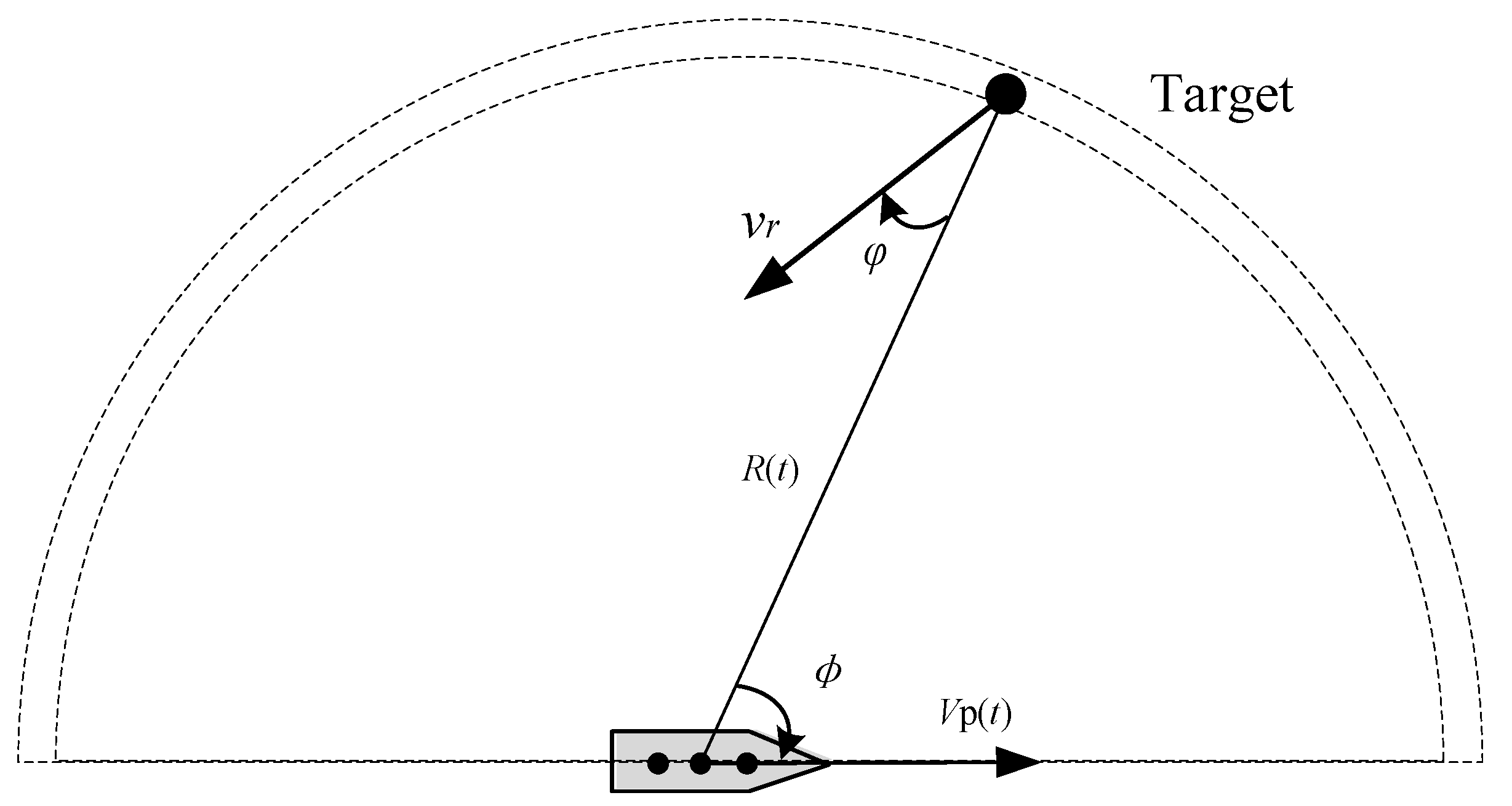
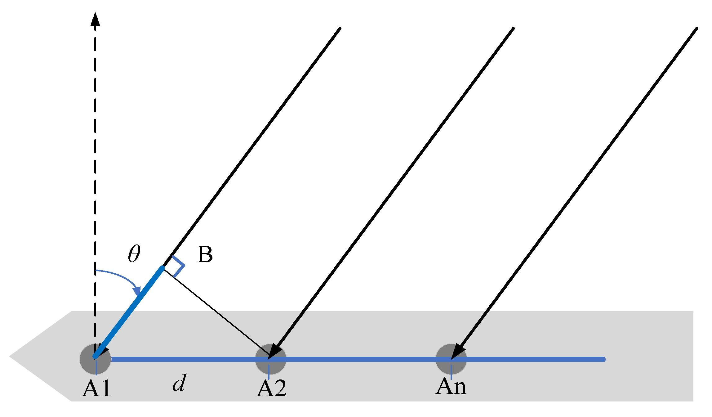
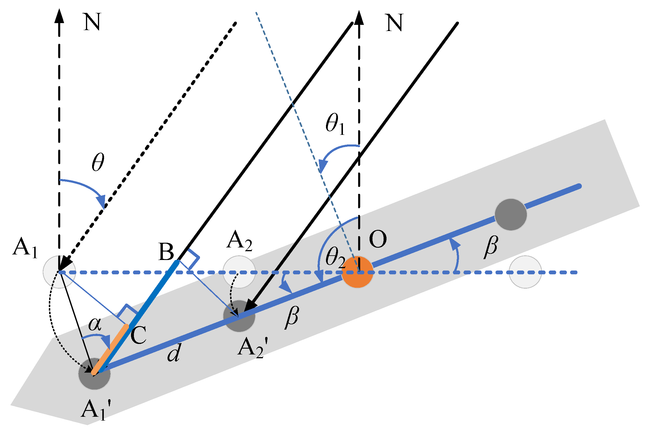
2. Target Echo Model for HFSWR on a Sailing Ship

Figure 1 shows the schematic diagram of target detection using shipborne HFSWR, and Figure 2 illustrates the physical model of the shipborne HFSWR platform.

For shipborne HFSWR, the transmitting and receiving stations are both on the ship. Assume N receiving antennas are equally spaced by a distance d along one side of the ship, the y-direction is in the normal direction of HFSWR array, and the antenna element located is selected as the reference element, then the received signal on the reference array element can be expressed as follows:

$$x_1\left(t\right)=s\left(t\right)+n_1\left(t\right)$$

(1)

where $n_1\left(t\right)$ is the additive noise of the reference array element. The phase difference between adjacent array elements is $2\pi d\sin \theta /\lambda$, and the received signal on the mth element is

$$x_m\left(t\right)=s\left(t\right)e^{j2\pi \left(m-1\right)d\sin \theta /\lambda }+n_m\left(t\right)$$

(2)

where $\lambda$ is the wavelength of the radar signal, and $\theta$ is the direction of arrival (DOA) of the target signal. Then, the steering vector can be obtained as

$$a\left(\theta \right)={[\begin{array}{cccc}1& e^{j2\pi d\sin \theta /\lambda }& \cdots & e^{j2\pi \left(N-1\right)d\sin \theta /\lambda }\end{array}]}^T$$

(3)

Thus, the received signal of the N-element array is

$$x\left(t\right)=\left[\begin{array}{c}\begin{array}{c}1\\ e^{j2\pi d\sin \theta /\lambda }\\ \dots \end{array}\\ e^{j2\pi \left(N-1\right)d\sin \theta /\lambda }\end{array}\right]s\left(t\right)+\left[\begin{array}{c}\begin{array}{c}{n}_1\left(t\right)\\ n_2\left(t\right)\\ \dots \end{array}\\ n_N\left(t\right)\end{array}\right]$$

(4)

For the first element in the receiving antenna array, $s_i\left(t\right)=A{e}^{j\mathsf{\Omega }t}$, in which, $e^{j\mathsf{\Omega }t}=e^{j2\pi f_{d}t}$ is the phase change caused by the Doppler offset $f_d$ of the target relative to the shipborne platform, and $A$ is the amplitude of the target echo. When the ship motion is linear, the receiving position of the array element changes due to the position variation of the platform, this change can be reflected in the steering vector. The Doppler frequency shift of a moving target is caused by the relative velocity between the target moving platform. Thus, the echo Doppler frequency $f_d$ can be computed as

$$f_d=\frac{2v_r}{\lambda }\cos \phi +\frac{2v_p\left(t\right)}{\lambda }\cos \varphi =f_{dr}+f_{dp}$$

(5)

in which, $v_r$ is the target velocity, $v_p\left(t\right)$ is the ship velocity, φ is the angle between the target heading and the echo DOA, and $\varphi$ is the angle between the ship heading and the target echo DOA. It can be seen that the target Doppler frequency shift consists of two parts, one is the Doppler offset $f_{dr}=\frac{2v_r}{\lambda }\cos \phi$, which is caused by the target velocity, and the other is $f_{dp}=\frac{2v_p\left(t\right)\cos \varphi }{\lambda }$, which is the echo Doppler offset caused by the forward linear motion of the ship itself. The target echo amplitude $A$ mainly depends on the scattering cross-sectional area and the target range from the ship, as the cross-section of the target is mainly determined by its relevant parameters, such as target size, tonnage and superstructure, and radar frequency [23]. The echo amplitude of target to be detected can be set to a fixed value under the condition of constant radar frequency and detection range. When the yaw occurs during the sailing, the heading of the shipborne platform will change, as shown in Figure 3, in which, ${\theta }_1$ is the spindle angle (the angle between the true North and the broadside direction of the ship) of the radar receiving station, and ${\theta }_2$ is the heading of the ship, and it can be found ${\theta }_1$ = ${\theta }_2$ + 90.

Assuming that the antenna array yaw along point $O$ when the heading $\phi$ changes and the yaw angle is $\beta$, the Doppler shift of the moving target can be calculated as

$$f_d=\frac{2v_r}{\lambda }\cos \phi +\frac{2v_p\left(t\right)}{\lambda }\sin \left(\theta +\beta \right)$$

(6)

Then, the distance between the first station element $A_1$ and point $O$ is $A_1^{\prime }O=\left(\frac{N-1}{2}\right)d$, and the displacement of $A_1$ is

$$A_1^{\prime }C=A_1^{\prime }{A}_1\cos \alpha$$

(7)

where $A_1^{\prime }{A}_1=2A_1^{\prime }O\sin \left(\frac{\beta }{2}\right)$, and $\alpha =\frac{\beta }{2}+\theta$, then

$$A_1^{\prime }C=2A_1^{\prime }O\sin \left(\frac{\beta }{2}\right)\cos \left(\frac{\beta }{2}+\theta \right)$$

(8)

The phase change between the two adjacent elements is

$$A_1^{\prime }B=d\sin \left(\theta +\beta \right)$$

(9)

According to (8), it can be seen that when the yaw angle is β, the azimuth angle of the target will change from θ to θ + β. Therefore, it can also be concluded that when the heading changes, it will certainly affect the measurement of the target azimuth. Based on (7) and (8), the steering vector considering the yaw effect can be obtained as

$$a{\left(\theta \right)}^{\prime }={[\begin{array}{cccc}{e}^{j2\pi d^{\prime }/\lambda }& e^{j2\pi \left(d^{\prime }+d\sin \left(\theta +\beta \right)\right)/\lambda }& \cdots & e^{j2\pi \left(d^{\prime }+\left(N-1\right)d\sin \left(\theta +\beta \right)\right)/\lambda }\end{array}]}^T$$

(10)

where $d^{\prime }=\left(N+1\right)d\sin \left(\frac{\beta }{2}\right)\cos \left(\frac{\beta }{2}+\theta \right)$. When β = 0, the steering vector is simplified to Equation (3), which is the case for linear motion.

Similar to the analysis of periodic yaw motion, other periodic motion such as roll and pitch can be further analyzed. It should be noted that, during sailing, the stability of the shipborne platform can be maintained by changing the velocity or direction according to the actual sea conditions, and the amplitude of rolling and pitching can be reduced as much as possible. Therefore, this study only focuses on the simulating target echo when the ship is sailing with yaw motion in the next section.

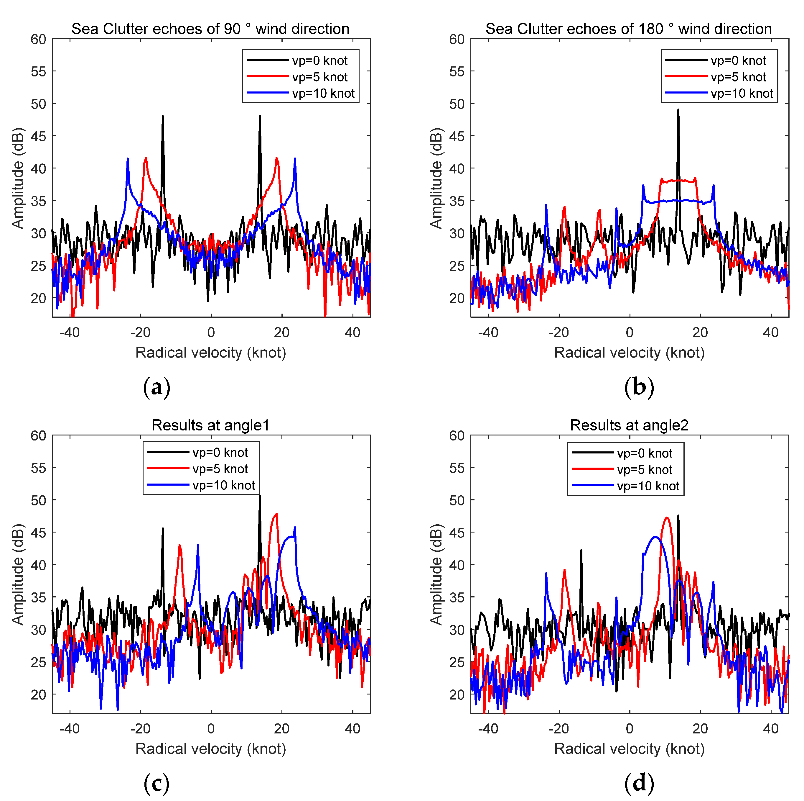
3. Simulation of Vessel Target Echo for Shipborne HFSWR during Sailing

Two vessel targets T1 and T2 are selected as examples for simulation here. Their azimuths are at −60°and 40°, respectively, i.e., $\theta 1=-60°$, $\theta 2=40°$. Their velocities are both 8 knots, while their headings are 0° and 180°, respectively. It should be noted that in the simulation, the heading and ship sailing direction are the same, and the difference between them is ignored here. In the simulation analysis, the same configuration parameters as those of an actual HF radar hardware system (see Section 6 for details) are used: the radar frequency is 4.7 MHz, the bandwidth is 60 k, the array element spacing is 17 m, the number of array elements is 8, and the pulse repetition period is 0.128 s.

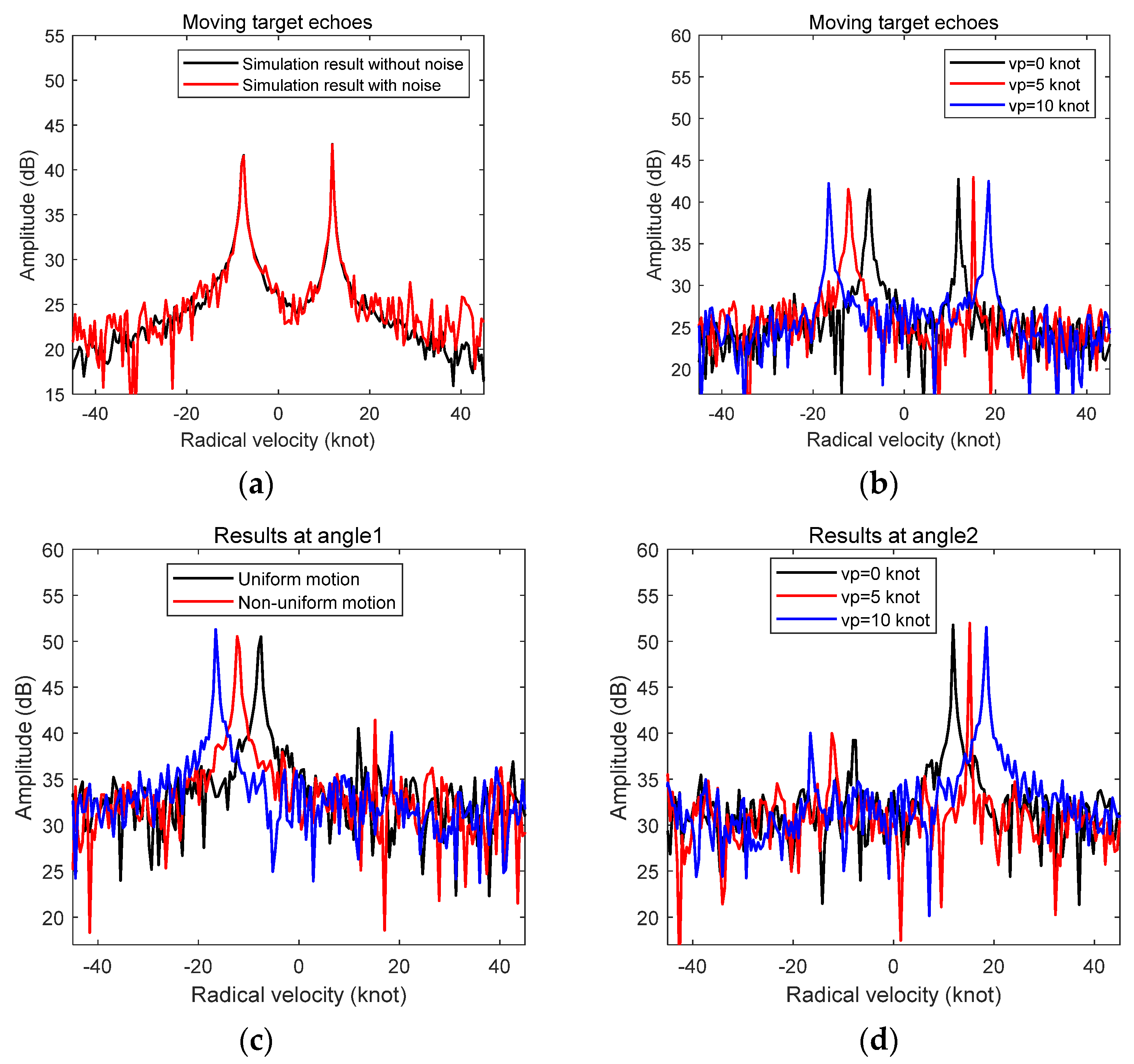
3.1. Simulation in the Case of Straight-Line Sailing

Figure 4b shows the simulation results of the target echoes when the ship motion is uniform linear with a velocity $v_p$ of 0, 5, and 10 knots, respectively. It can be seen from Figure 4a that when the velocity of the platform is 0 knots, the Doppler shift of a moving target echo is mainly determined by its own moving velocity, and both target echo peaks are obvious with high SNR. When the ship sails at a constant velocity, the echo amplitude and the SNR of the two targets remain unchanged in both the channel spectrum and beam spectrum after beamforming, but the position of the target peak in the spectrum changes. It indicates that the target echoes only have frequency shift without broadening, and the frequency shift is determined by the target motion velocity and platform velocity, as specified in (5).

As we know, in the case of uniform linear platform motion, the first-order sea clutter spectrum of a shipborne radar will be broadened, and its broadening width increases with the increase in platform velocity, as shown in Figure 5. Compared with the channel spectrum, the sea clutter in the beam spectrum in a certain direction is still broadened, but the broadening width is narrower than that in the channel spectrum. The difference between the target echo and sea clutter is due to the fact that a moving target usually exists only in one range cell and in one certain direction, whereas sea echoes appear in multiple cells in each direction. As the Doppler shift of sea surface echoes from different directions are different under the influence of the platform motion, the sea clutter spectrum in the channel data is broadened. As for the beam spectrum, which is obtained after beamforming multi-channel data, the sea clutter in the beam will be broadened due to the large beam width of HF radar.

It should be noted that the broadening of the sea clutter caused by platform motion will increase the influence width of the blind area caused by the sea clutter, which is detrimental to target detection. However, the amplitude of the sea clutter spectrum decreases with its broadening, which may be beneficial to the detection of a target that was originally submerged in sea clutter.

The simulation results of the target echo for HFSWR on a ship with non-uniform linear motion are displayed in Figure 6. Figure 6a shows that the ship velocity decreases from 10 knots to 5 knots with a constant deceleration. While for the results in Figure 7, the ship velocity changes periodically with a period P = 10 s.

It can be seen from Figure 6b that the echoes of the two moving targets are broadened and the SNR of the target in the case of ship with uniform deceleration motion is significantly lower than that with uniform motion. After beamforming, although the SNRs of the two targets are improved to some extent, the broadening width of the target echo does not change. Moreover, the SNR of the target is still significantly lower in the case of non-uniform motion compared to uniform motion. In contrast, the broadening of sea clutter can be appropriately reduced after beamforming. Therefore, non-uniform linear motion that can result in broadening of the target signal and reduction in SNR is detrimental to target detection.

As can be seen from Figure 7b, when the ship velocity varies periodically, false target peaks appear at certain frequencies on both sides of the true target signal in both the channel and beam data, although the target echo spectrum is not broadened. The emergence of false peaks will cause false alarms and affect the detection performance.

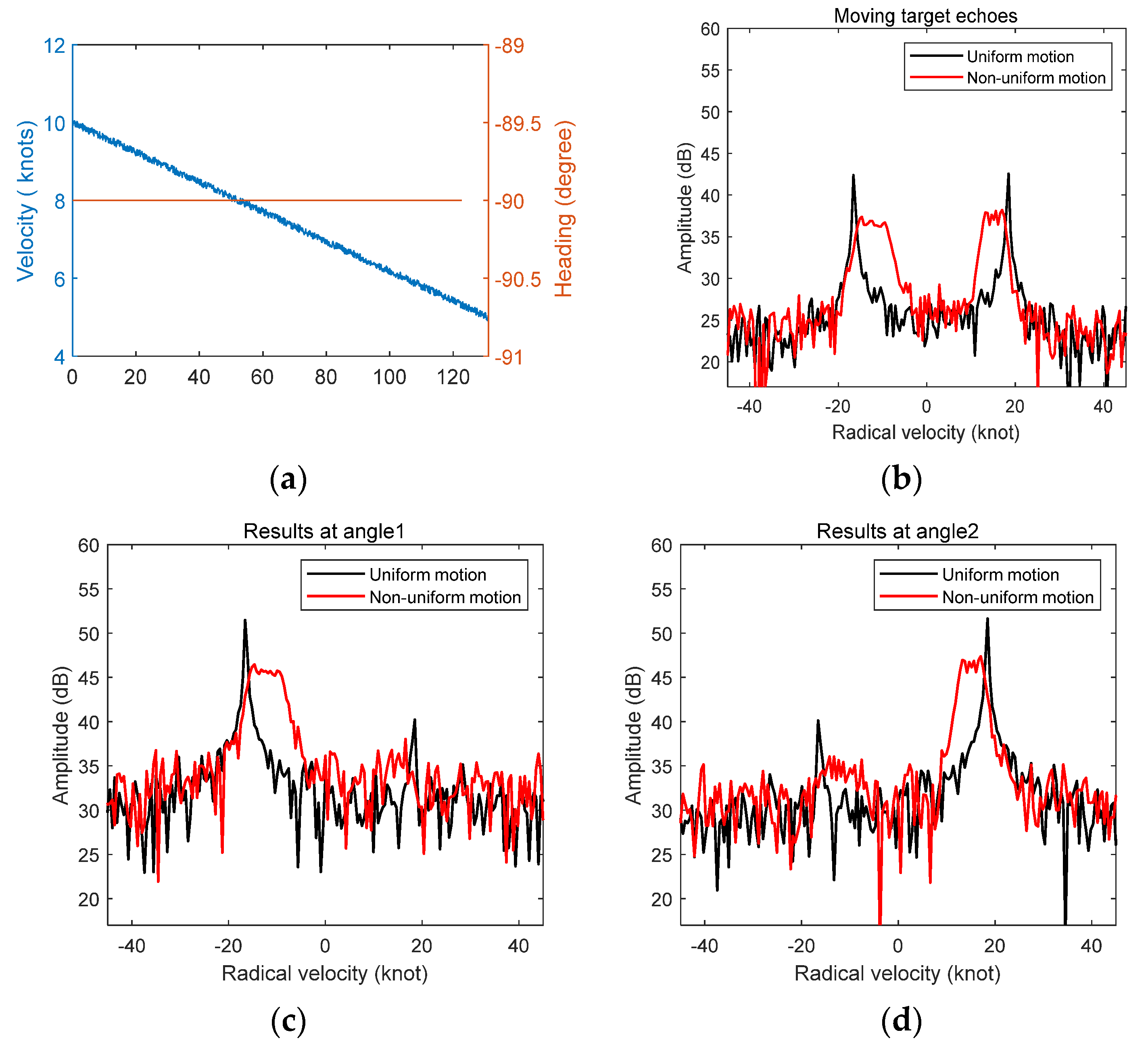
3.2. Simulation in the Case of Yaw Motion

Figure 8 depicts the simulation results of the target echo when the ship undertakes yaw motion. The ship velocity is constant during the accumulation time, while the heading is uniformly adjusted from −90° to −120°, i.e., the yaw angle β is −30°. With the effect of the yaw motion, the bearings of the two targets are −90° and 10°, respectively, in the radar coordinates.

As can be seen from Figure 8, the echo spectrum of the moving target will also be broadened if the ship heading changes at a uniform rate, which is similar to the situation of linear sailing with uniform acceleration. Figure 9 shows the simulation results when the yaw angle varies periodically with a period of 20s and a swing amplitude of 5°. In order to compare the spectra while the ship is sailing and at anchor state, the simulation results of target 1 with a velocity of $V_p=0$ and $V_p=10$ are shown in terms of beam data.

As can be seen from Figure 9 that the amplitude of the target echo is almost unchanged when the heading changes periodically with a velocity of 0 knots. In addition to the true target signal, some false peaks appear on both sides, and their amplitudes are obviously lower than that of the real target and decrease rapidly to the noise floor level. However, the amplitudes of the false peaks on both sides of the true target echo are decreasing slowly when the ship velocity is 10 knot. In addition, the echo amplitude of the target is significantly lower than that without heading change, while the amplitude is comparable to that of the false peaks on its both sides. In this case, it is more difficult to detect the target signal.

Figure 10 depicts the simulated results of the target echo for the case in which both the ship velocity and heading change. The heading is uniformly adjusted from −90° to −40°, i.e., the yaw angle β is 50°. With the effect of the yaw motion, the bearings of the two targets are 10° and 90°, respectively, in the radar coordinates. In the meantime, the ship velocity increases from 0 knots to 10 knots with a constant acceleration, and then, it decreases from 10 knots to 0 knots with a constant deceleration. As can be seen from Figure 10, the echoes of the two targets are broadened when both the heading and velocity of the ship change, and the degree of broadening is obviously greater than that when only velocity or yaw angle change.

From the above theoretical and simulation analysis, it can be concluded that the ship velocity change or the heading change during the sailing can lead to the broadening of target echoes or the appearance of false target peaks in the shipborne HFSWR data. As a result, the target SNR will decrease, affecting the target detection performance and target parameter estimation accuracy. Since it is impossible to keep the ship moving at a uniform velocity along a straight line all the time during sailing, the influence of non-uniform ship motion on the Doppler spectrum of moving targets must be considered. Therefore, motion compensation is required before target detection to mitigate the effect of platform motion on target echoes.

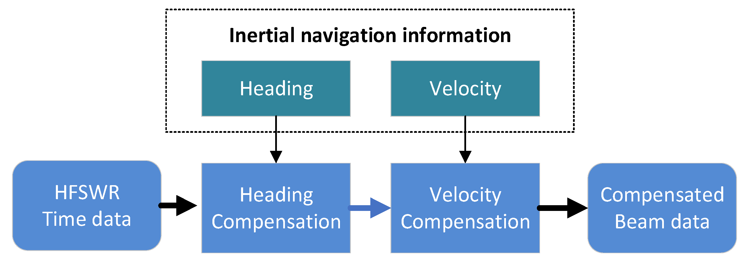
4. Motion Compensation of Target Echo for Shipborne HFSWR

Motion compensation for mitigating the influence of the shipborne platform motion on target echo is to reduce target signal broadening or false peaks caused by non-uniform motion. In order to realize the motion compensation of target echo for shipborne HFSWR under sailing, it is critical to compensate for the phase change generated by the platform motion. From the analysis in Section 2, it can be seen that the phase change in the target echo is mainly caused by the change in ship velocity and heading. Therefore, the motion compensation of shipborne HFSWR should include two steps: heading compensation and velocity compensation. The flow chart of shipborne radar motion compensation is shown in Figure 11.

In this process, the input data include multi-channel time-domain radar data and attitude information of the ship collected by the onboard inertial navigation equipment, in which the velocity and the heading information of the ship are included.

The first step is heading compensation. In this step, the output is the compensated beam data. Based on the heading information, the spindle angle of the radar receiving station ${\phi }_t$ in the coherent integration time can be calculated. By setting the spindle angle of the beginning time $t0$ as the benchmark and calculating the change in the radar spindle angle relative to the reference time, i.e., the yaw angle $\beta$ at each moment can be found as

$$\beta ={\phi }_t-{\phi }_{t0}$$

(11)

Then, the compensated steering vector $b\left(\theta \right)$ at beam angle $\theta$ can be constructed based on the estimated yaw angle $\beta$ as

$$b\left(\theta \right)={[\begin{array}{cccc}{e}^{-j2\pi d^{\prime }/\lambda }& e^{j-2\pi \left(d^{\prime }+d\sin \left(\theta +\beta \right)\right)/\lambda }& \cdots & e^{-j2\pi \left(d^{\prime }+\left(N-1\right)d\sin \left(\theta +\beta \right)\right)/\lambda }\end{array}]}^T$$

(12)

in which $d^{\prime }=\left(N+1\right)d\sin \left(\frac{\beta }{2}\right)\cos \left(\frac{\beta }{2}+\theta \right)$. Based on $b\left(\theta \right)$, the target signal after heading compensation can be estimated as

$$x{\left(t\right)}^{\prime }=x\left(t\right)b{\left(\theta \right)}^{\mathrm{T}}$$

(13)

The second step is velocity compensation, which is realized according to (14)

$${\widehat{s}}_m\left(t\right)=s_m\left(t\right)\cdot e^{-2j\pi {\varphi }_{\theta }\left(t\right)}$$

(14)

where ${\varphi }_{\theta }\left(t\right)=\frac{2v_p\left(t\right)\cos (\raisebox{1ex}{$\pi $}\!\left/ \!\raisebox{-1ex}{$2$}\right.-\theta +\beta \left(t\right))t}{\lambda }$ is the phase offset of the target echo caused by the platform motion, as defined earlier, $\varphi$ is the angle between the echo direction and the platform motion direction, $v_p\left(t\right)$ is the real-time ship velocity, and $\beta \left(t\right)$ is the yaw angle at time t. Then, it can be compensated to the average velocity through

$$v_p{\left(t\right)}^{\prime }=v_p\left(t\right)+\mathsf{\Delta }{v}_p\left(t\right)$$

(15)

in which $\mathsf{\Delta }{v}_p\left(t\right)$ = $\overline{v_p\left(t\right)}-v_p\left(t\right)$ is the velocity difference between the target instantaneous velocity $v_p\left(t\right)$ and the average velocity $\overline{v_p\left(t\right)}$.

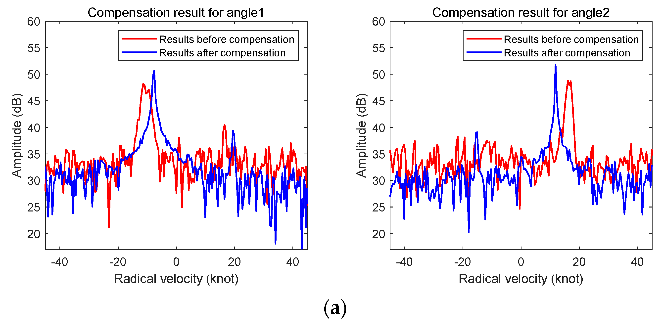
5. Simulation Analysis of Motion Compensation Results

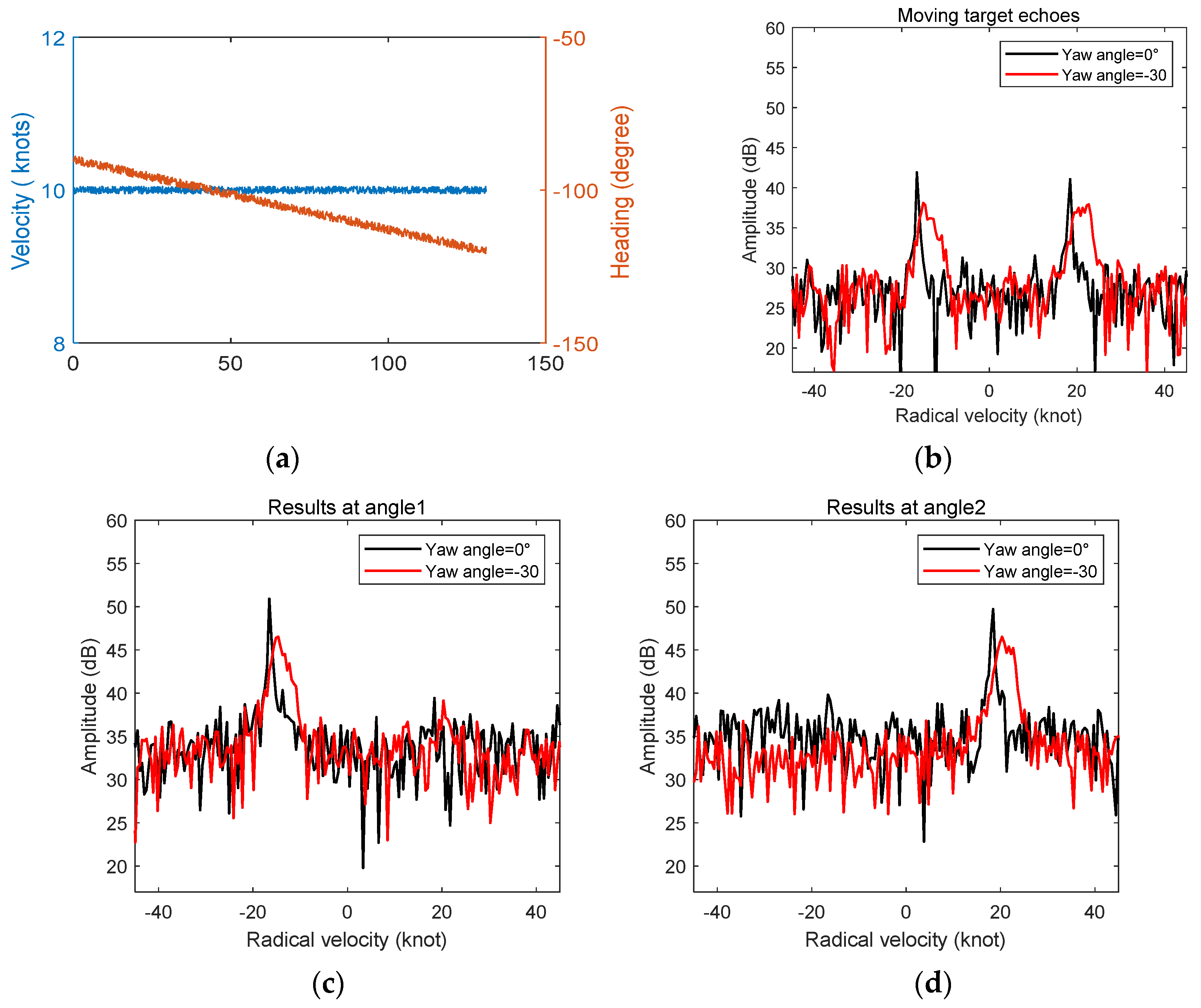
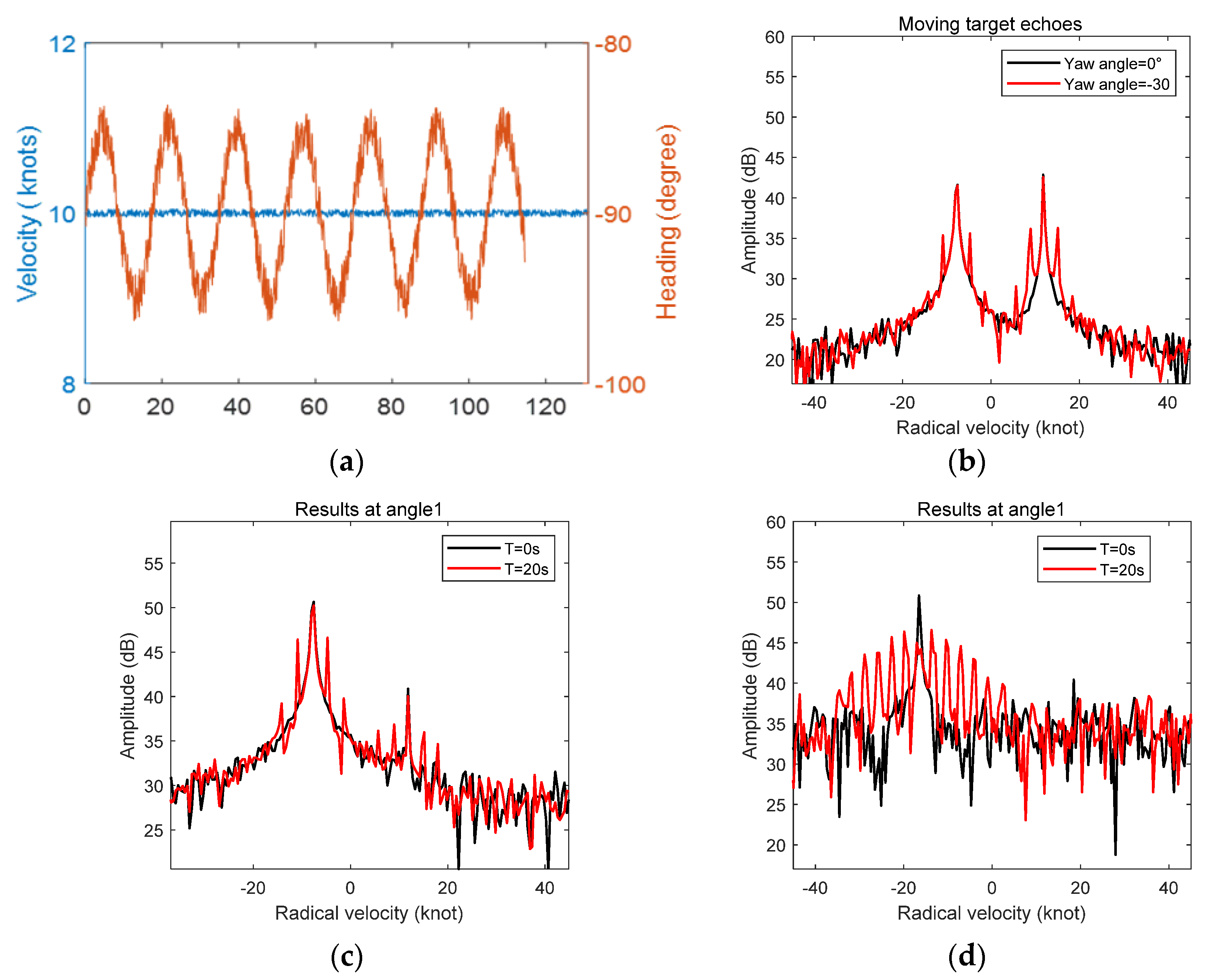
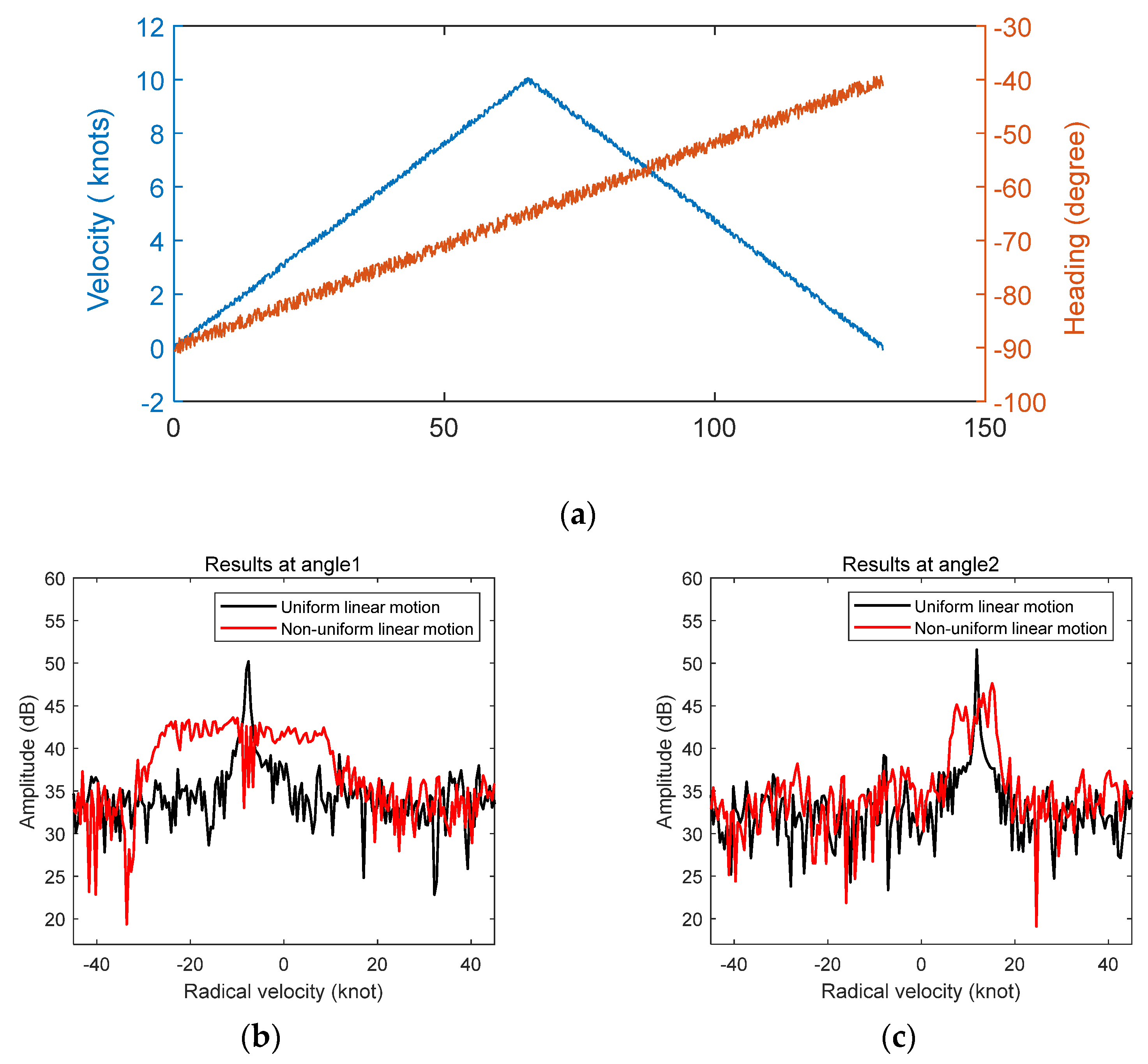
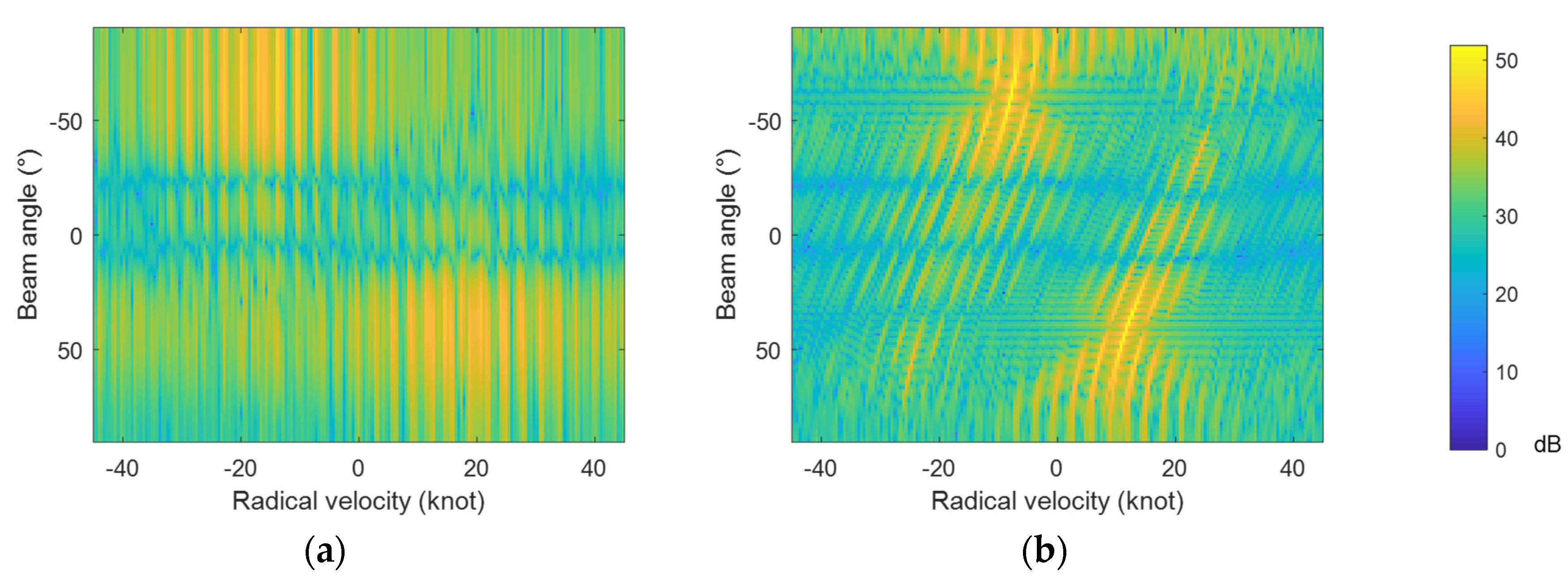
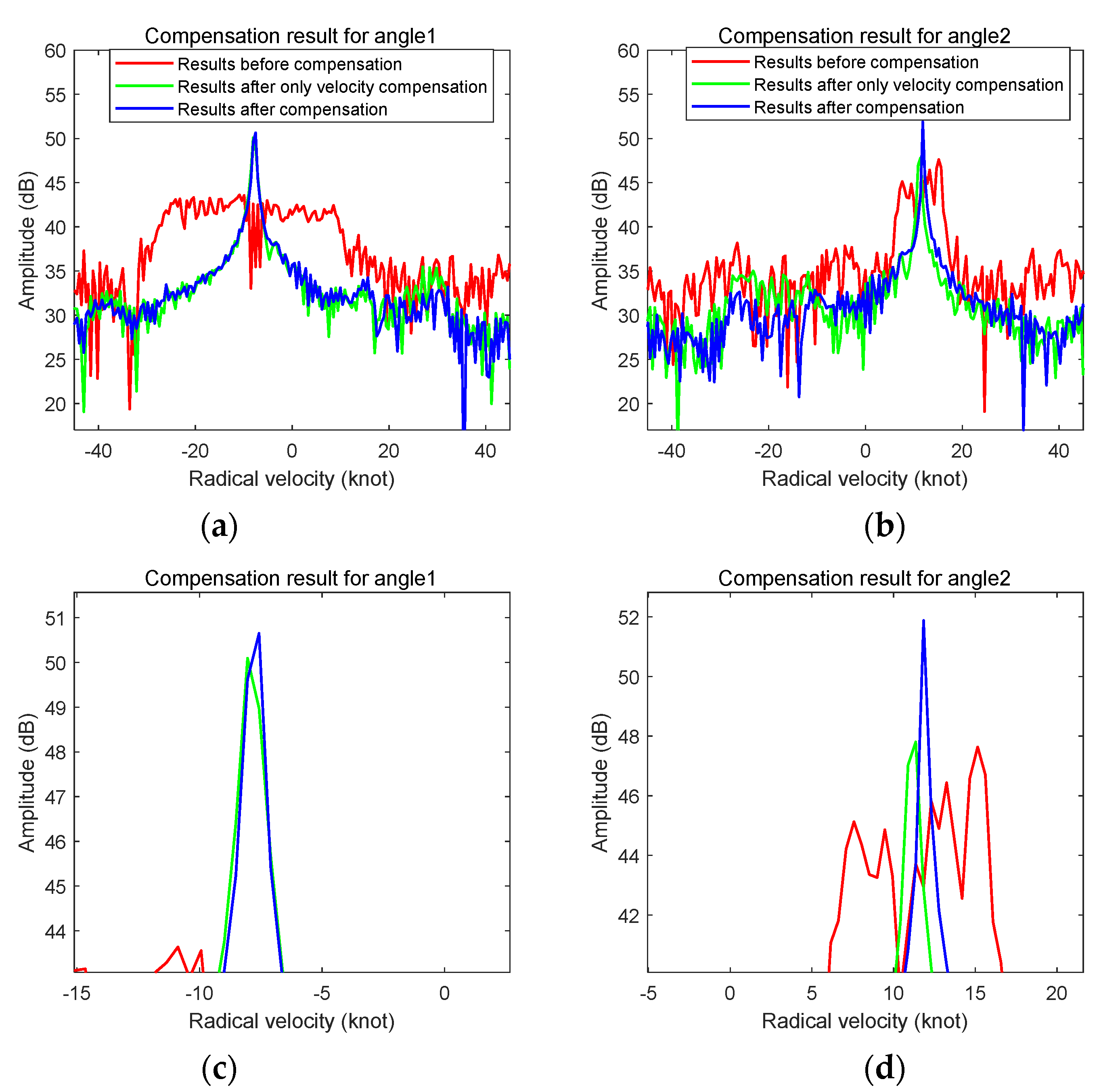
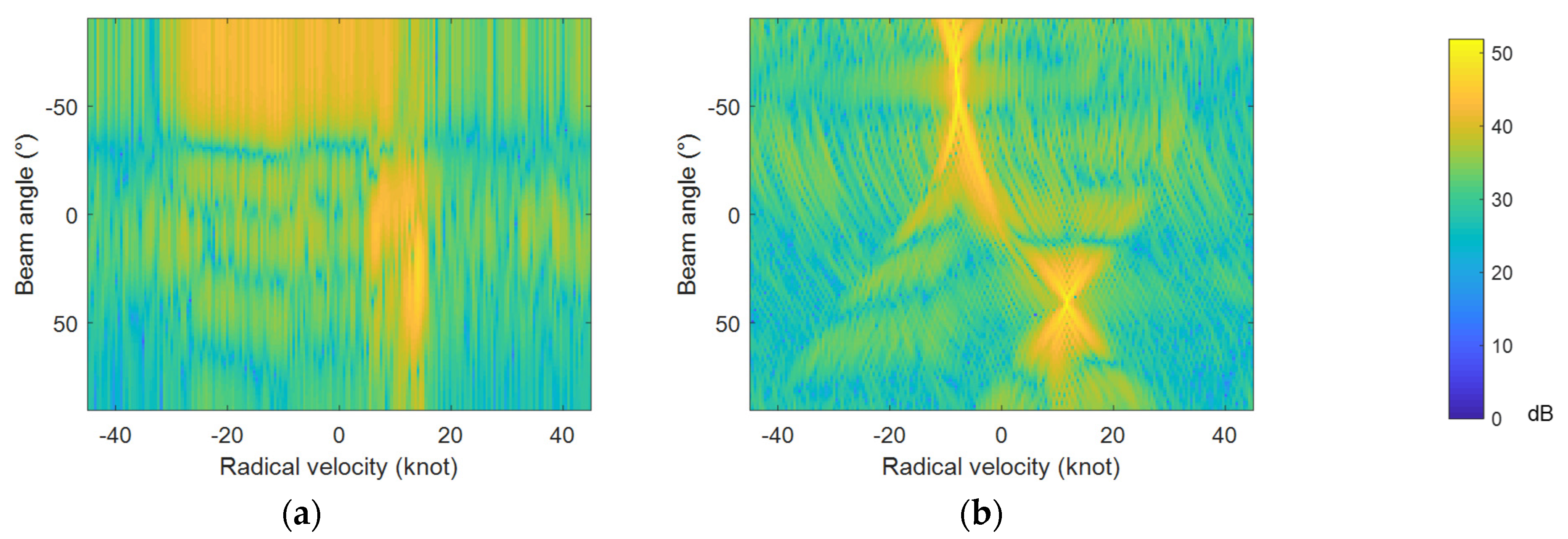
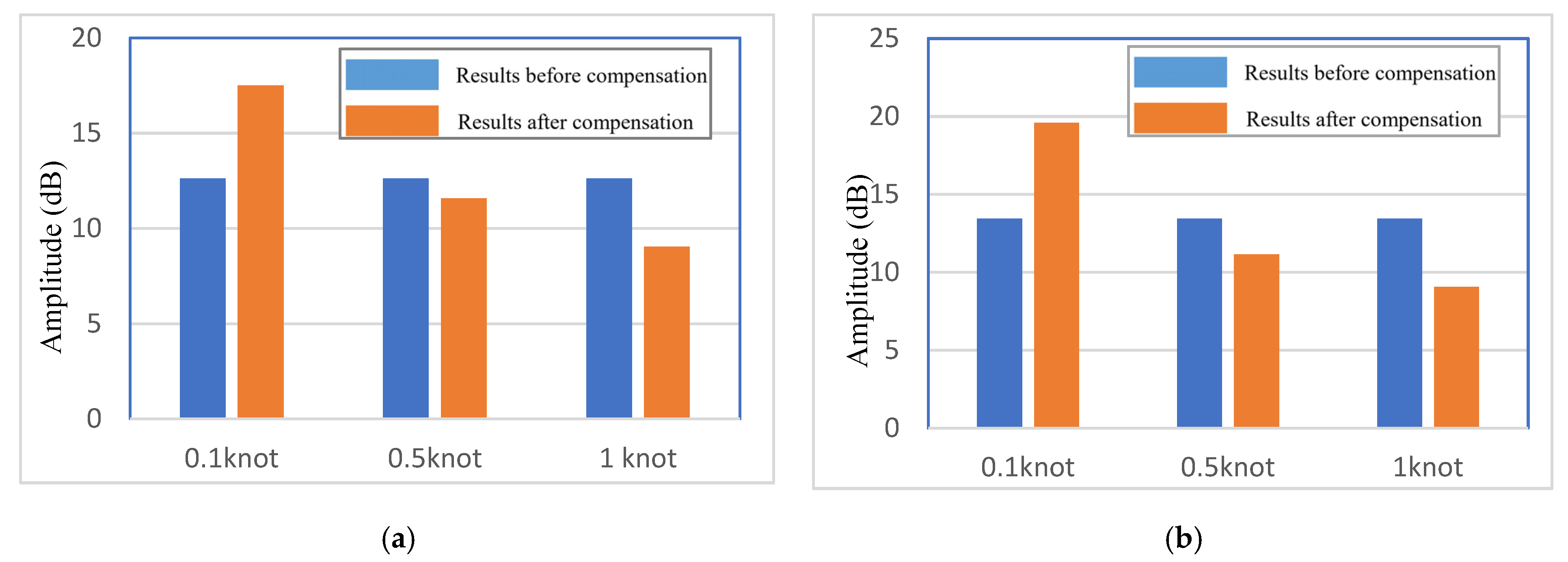
5.1. Motion Compensation Results for Non-Uniform Linear Motion

Figure 12 shows the results of motion compensation for a ship with uniform deceleration motion (non-uniform linear motion). Additionally, Figure 13 displays the space–time two-dimensional spectra before and after motion compensation. Similarly, Figure 14 depicts the motion compensation results for the case with uniform yaw with the velocity of 15 knots, 10 knots, and 15 knots, respectively. Figure 15 displays the space–time two-dimensional spectra before and after motion compensation when ship velocity is 10 knots. Figure 16 and Figure 17 show the motion compensation results for the case with periodic yaw motion and corresponding space–time two-dimensional spectra before and after motion compensation.

As can be seen from Figure 12 and Figure 14, the target echo spectrum after compensation for non-uniform linear motion or yaw motion is no longer broadened, and the SNR is obviously improved by about 5–15 dB, which is enough for target detection. It can also be seen from Figure 14 that the offset and broadening of target echo caused by different velocities are different, but their compensation results are almost the same.

Furthermore, from the space–time two-dimensional spectra in Figure 13 and Figure 15, it can be seen that the motion compensation results are favorable for the determination of target azimuth after eliminating target broadening and improving target SNR. Take target 2, for example, in the space–time two-dimensional spectrum before motion compensation, the target signal is distributed in the beam of 20° to 70° due to target signal broadening, making it difficult to determine the azimuth of the target. After motion compensation, the target signal becomes obvious at 40° in azimuth. As can be seen from Figure 16 and Figure 17, for the case in which yaw motion exists (e.g., Figure 9b, the yaw angle varies periodically with a period of 20 s and a swing amplitude of 5°), the improvement in target signal after motion compensation is more obvious, which not only improves the SNR, but also eliminates the false target peaks.

Figure 18 shows the results of motion compensation for the case with large variation in both ship velocity and heading (related to Figure 10), the velocity compensation results without heading compensation were also given for comparison in addition to the final compensation results (including velocity compensation and heading compensation). Figure 19 displays the space–time two-dimensional spectra before and after motion compensation. As can be seen from Figure 18, although the result with only velocity compensation can reduce the broadening of the target signal and improve the SNR, the amplitude of the compensated target echo is still lower than that of the processed result after heading and velocity compensation. Especially for target 2, the amplitude of the target signal is lower than about 4 dB. This proves that the heading compensation is beneficial to the improvement of the target signal.

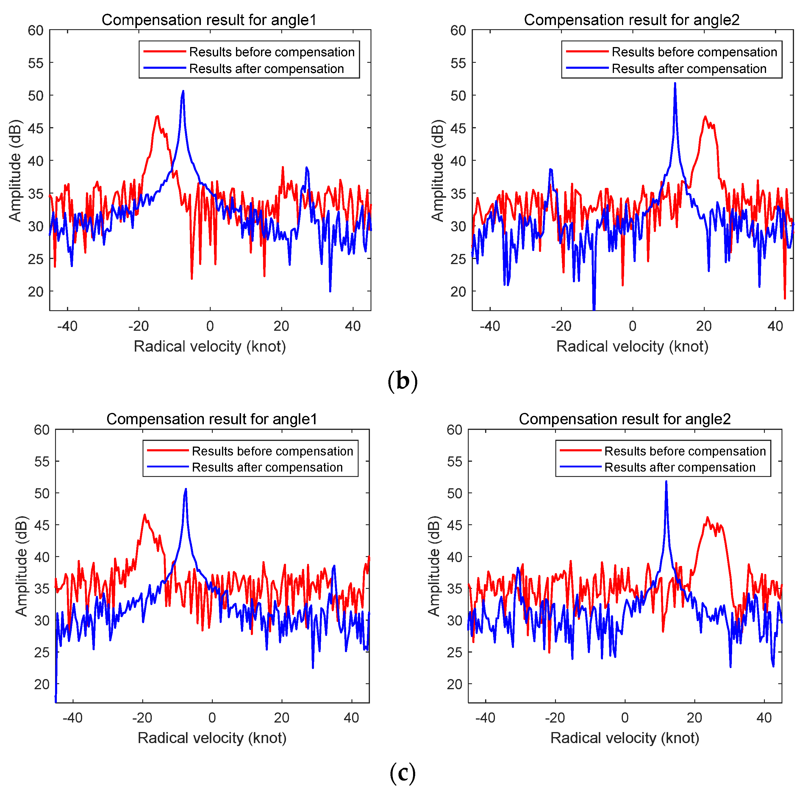
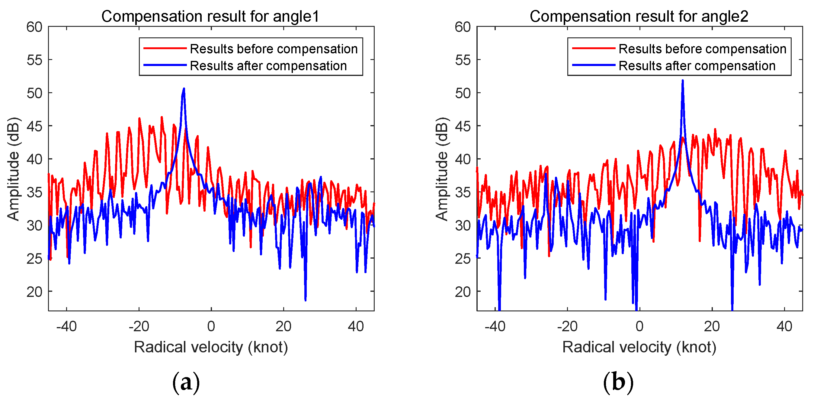
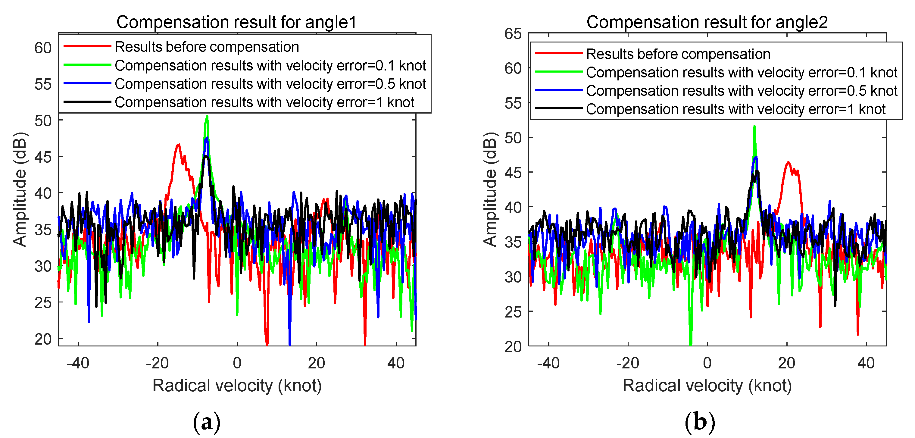
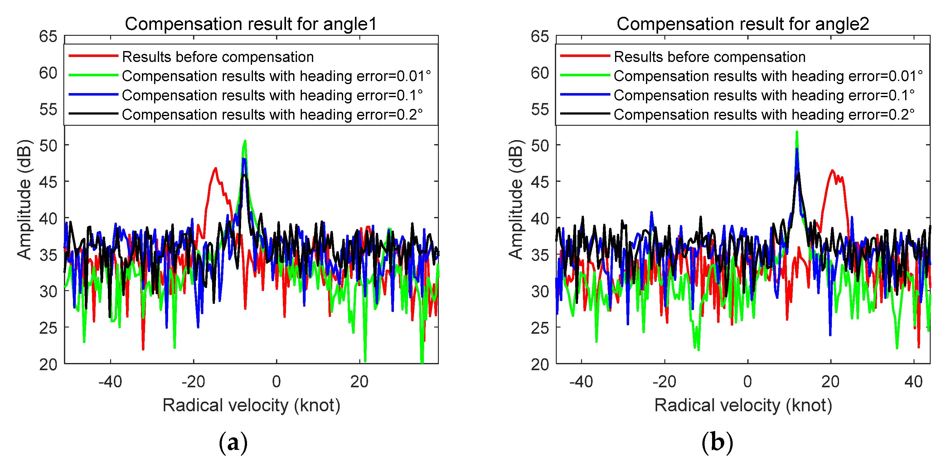
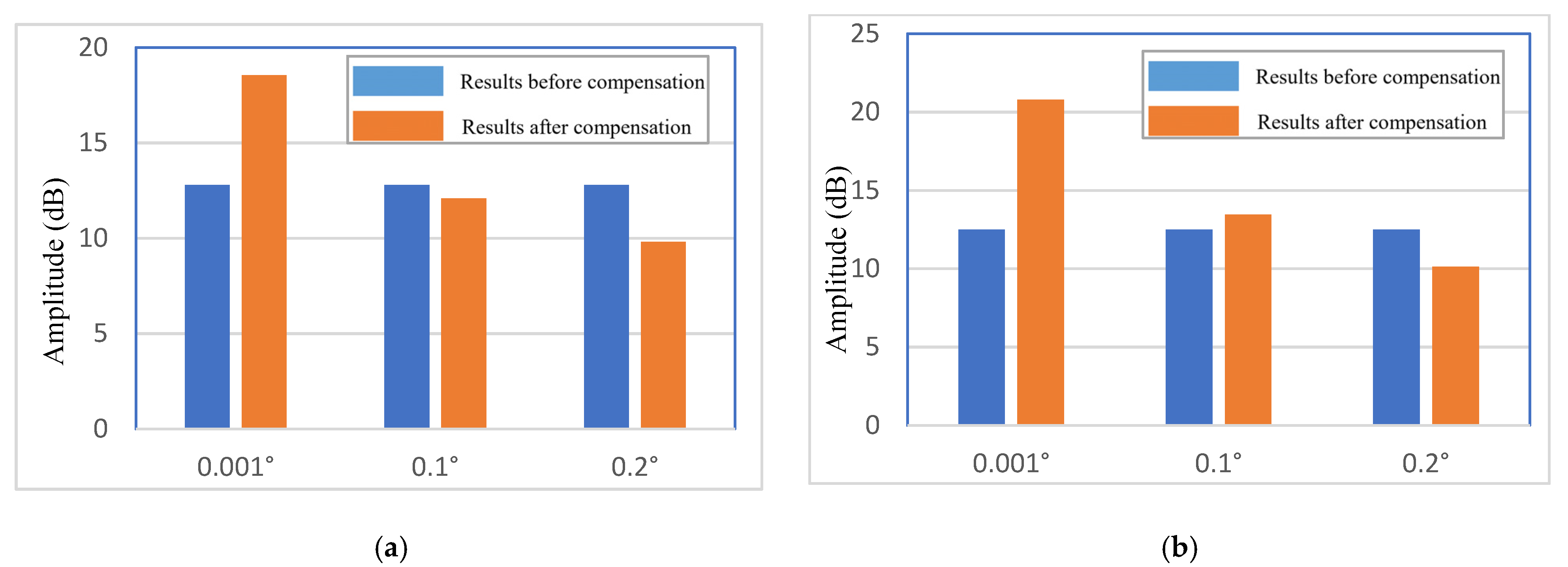
5.2. The Influence of Measurement Error on Motion Compensation Results

It is also necessary to analyze the influence of the velocity and heading measurement errors on the motion compensation results; thus, the simulation results of the motion compensation under different error conditions are presented. Here, the motion compensation results for the case of ship with yaw are selected as an example for analysis. Figure 20 shows the motion compensation results when the heading measurement is error free but the velocity measurement error is 0.1 knots, 0.5 knots, and 1 knot, respectively. Figure 21 illustrates the statistics of SNR for the two targets before and after motion compensation under different velocity measurement errors. Figure 22 shows the compensation results when the heading error is 0.01°, 0.1°, and 0.2°, respectively, but no velocity measurement error exists. Figure 23 depicts the statistical results of SNR for the two targets before and after motion compensation under different heading measurement errors. It should be noted that the error here refers to the standard deviation with a zero mean Gaussian distribution.

As can be seen from Figure 20 and Figure 21 that the SNRs of the two targets decrease to about 9 dB when the velocity error is increased to 1 knot. According to the above analysis, when there is no error in the heading measurement, the velocity estimation accuracy should be better than 0.5 knots, which cannot only eliminate the target echo broadening, but also improve the SNR of the target.

It can be observed from Figure 20 and Figure 21 that when the velocity measurement error is 0.1 knots, the SNRs of both targets after motion compensation were significantly higher than that before compensation. The SNR of target 1 was improved from 12.5 dB before compensation to 17.5 dB after compensation, and that of target 2 is also improved from 13.5 dB to 19.5 dB. When the velocity error reaches 0.5 knots, the SNRs of target 1 and target 2 were 11.5 dB and 11 dB, respectively, which were slightly lower than the SNR before motion compensation. When the error is reduced to 1 knot, the SNRs of the two targets decrease to about 9 dB, which is significantly lower than that before motion compensation. According to the above analysis, it can be concluded that the motion-compensated results can improve the SNR of the target via eliminating the spectrum widening of the target echo only if the velocity measurement accuracy is better than 0.5 knots.

It can be noticed from Figure 22 and Figure 23 that when the heading error is 0.01°, the SNR of the target after motion compensation is significantly higher than that before compensation, in which the SNR of target 1 is increased from 12.7 dB to 18.5 dB and that of target 2 is increased from 12.5 dB to 20.8 dB. When the heading error reaches 0.1°, the SNRs of target 1 and target 2 are reduced to 12.1 dB and 13.5 dB, which are comparable to the SNRs before motion compensation. When the error is increased to 0.2°, the SNRs of the two targets decrease obviously, which are only 10 dB and much lower than that before motion compensation. According to the above analysis, it can be concluded that when there is no error in the velocity measurement, the heading measurement accuracy should be better than 0.1° so that motion compensation is useful for improving the SNR.

It should be noted that the above accuracy analysis is obtained when the ship velocity is 10 knots. When the ship velocity changes, the accuracy may be different and further analysis is required. When both the velocity and heading measurement errors exist, the SNR of target echo after motion compensation will be lower than that with velocity error alone or heading error only. Therefore, in order to improve the signal-to-clutter ratio of the target echo for better target detection, it is necessary to use velocity and heading data with higher measurement accuracy.

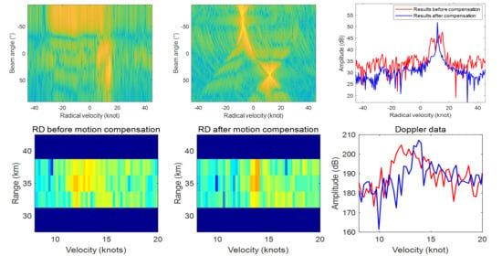
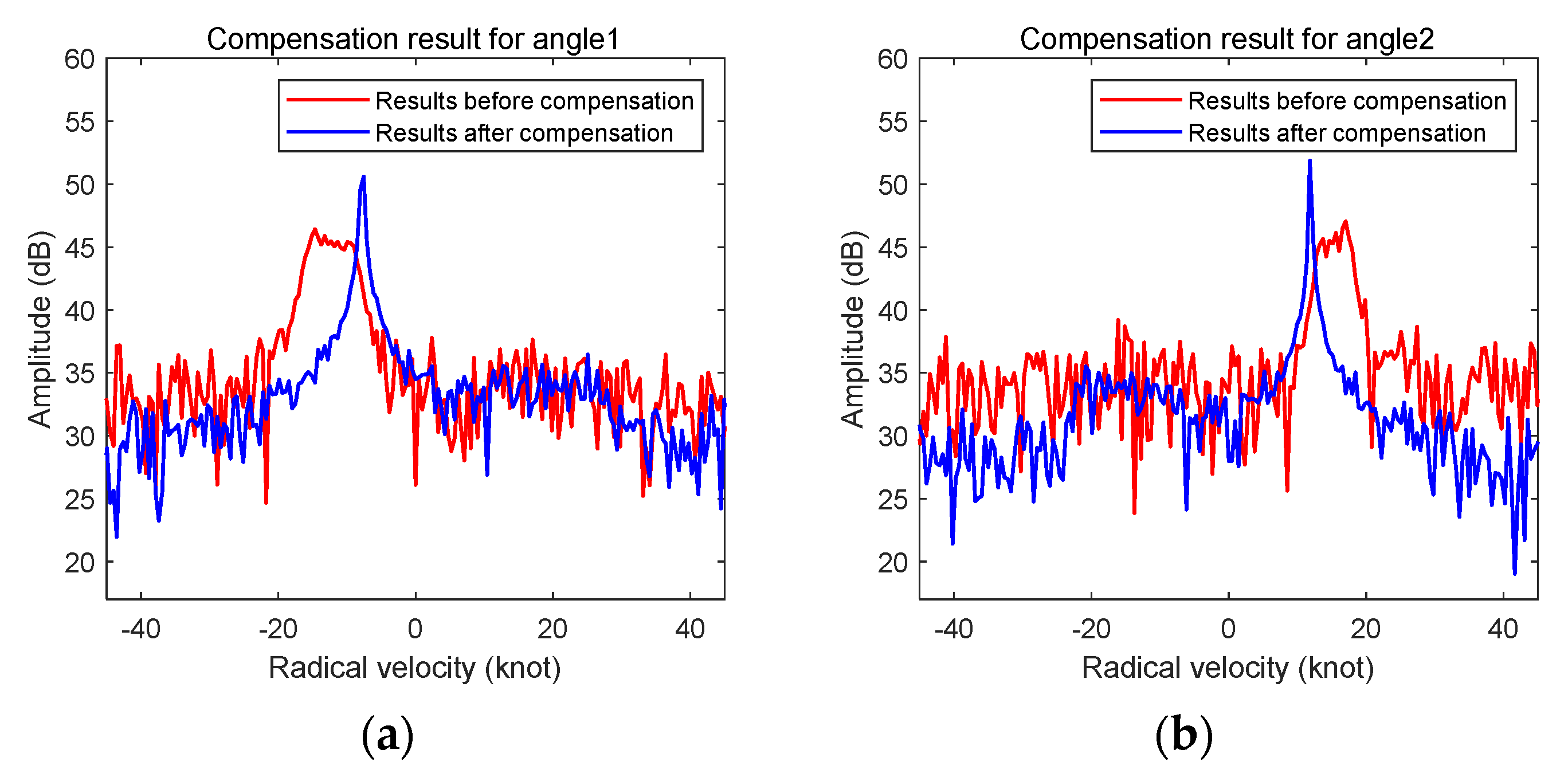
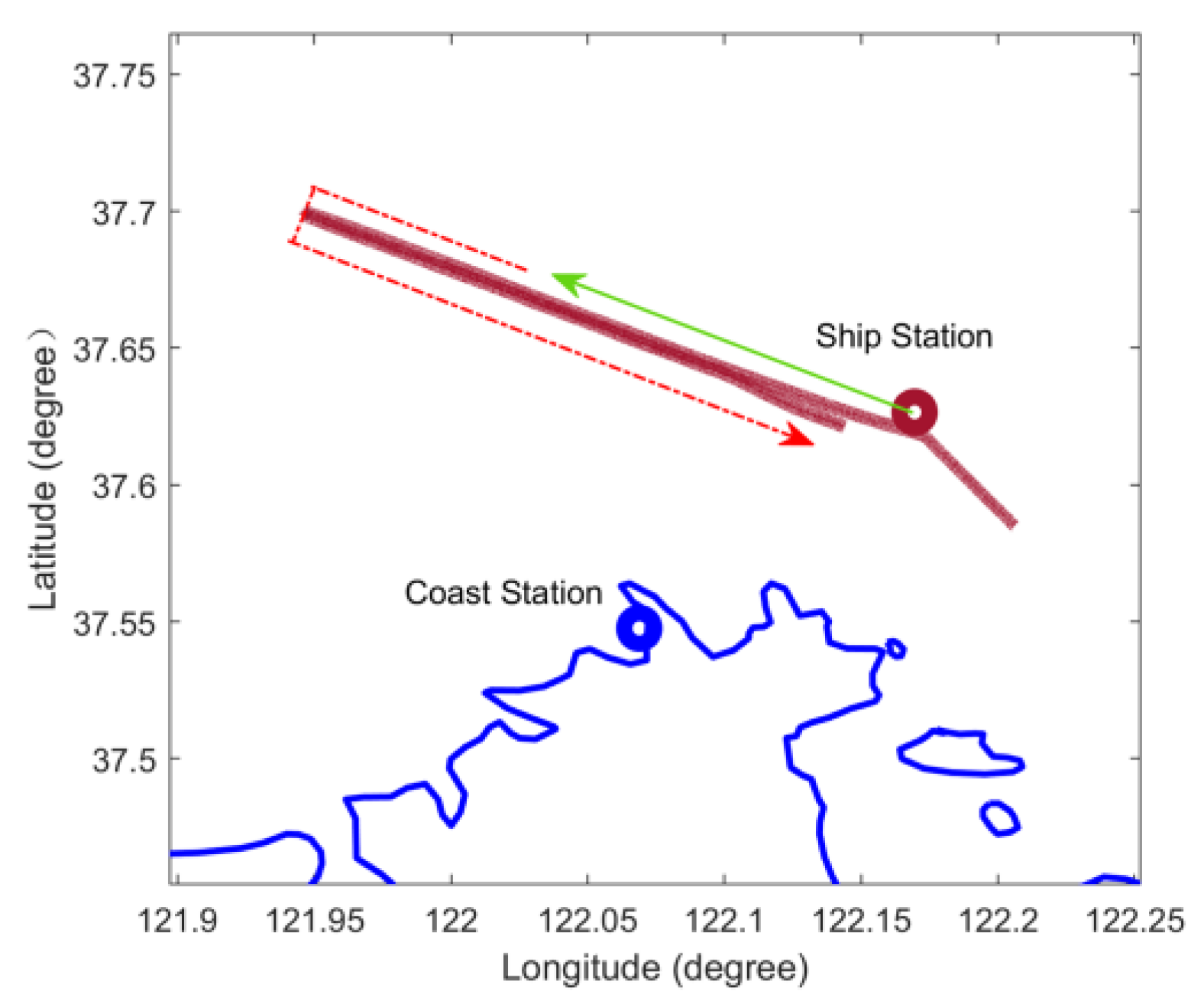
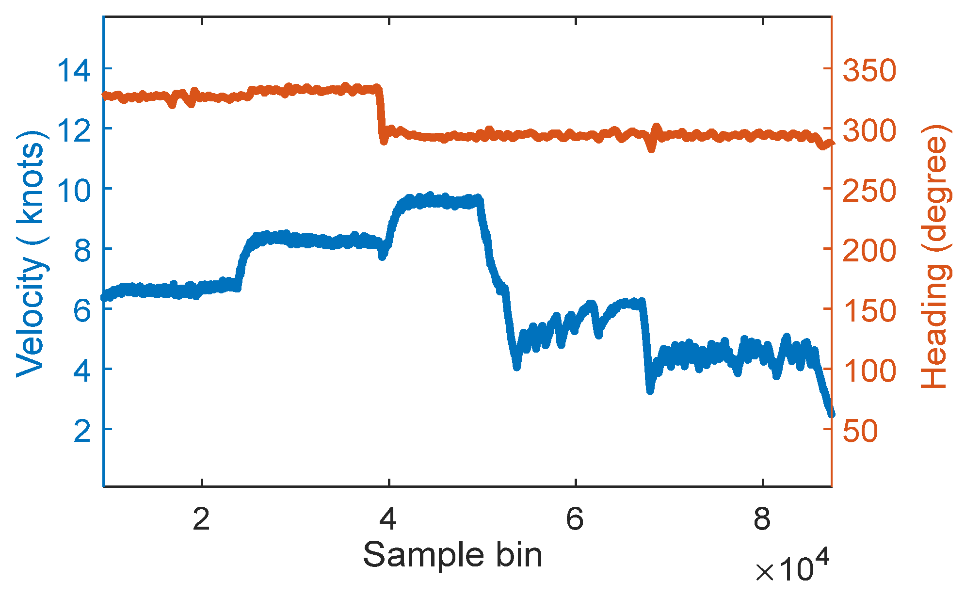
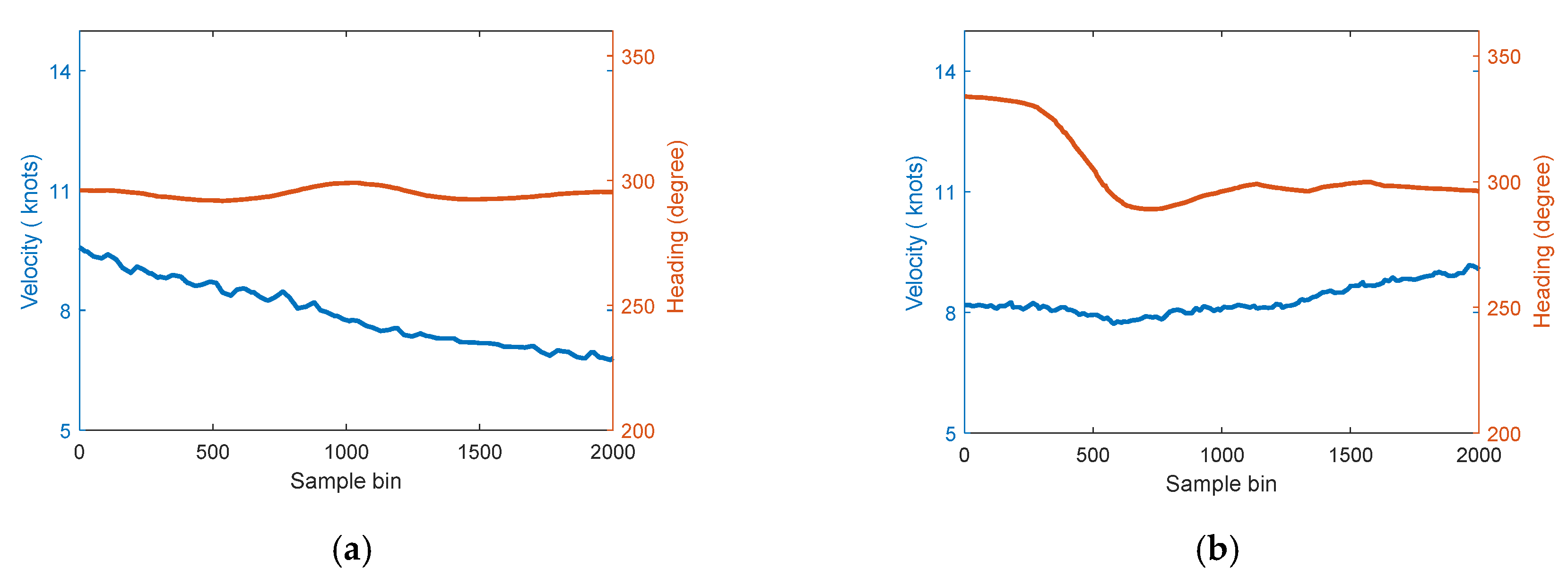
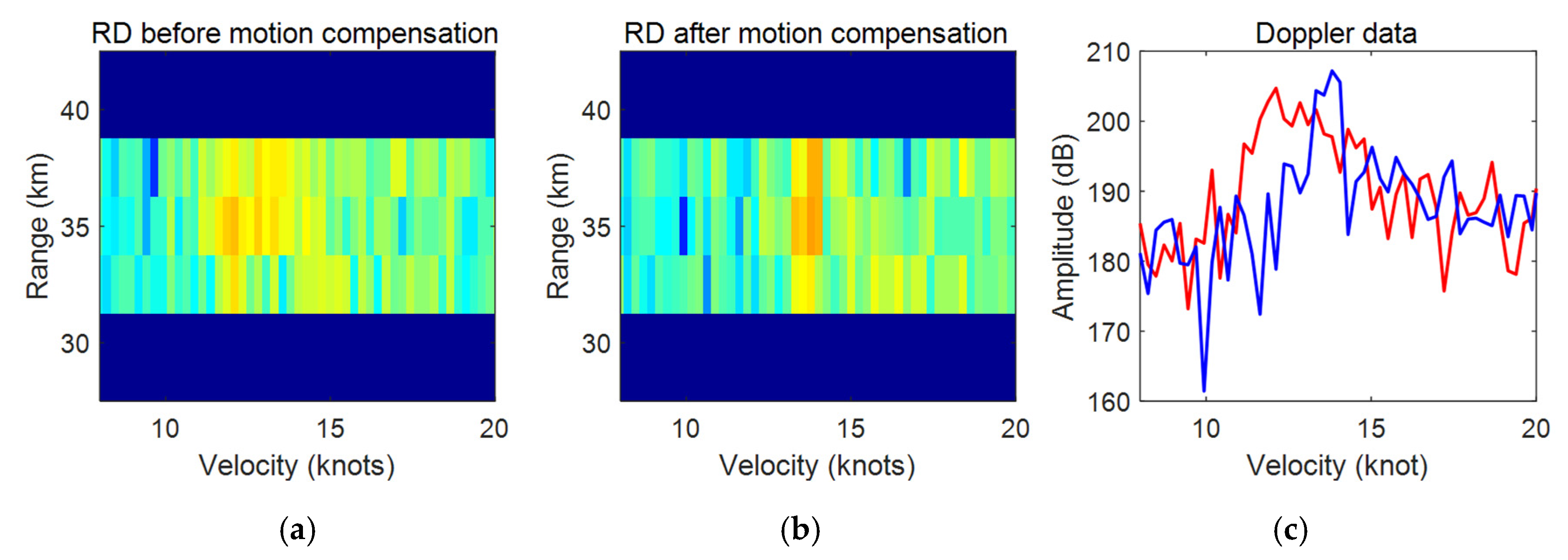
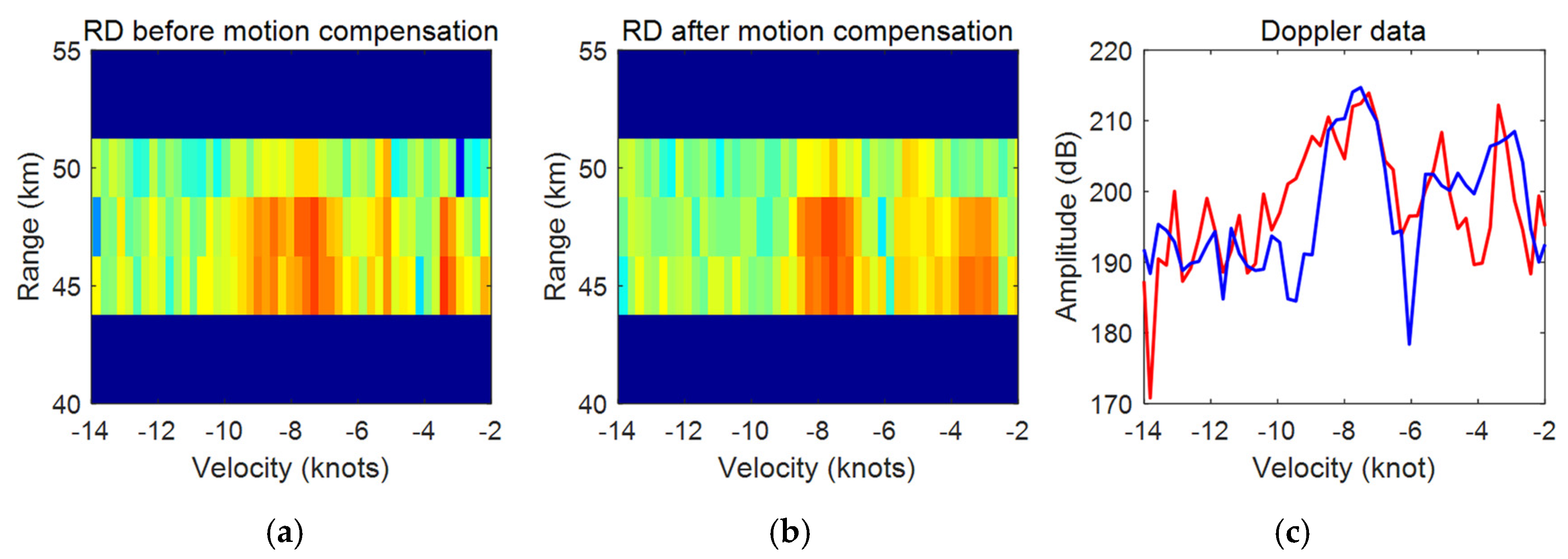
6. Validation with Measured Shipborne HFSWR Data

6.1. Description of the Shipborne HFSWR System

A shipborne HFSWR experiment was conducted in July 2019 using a Compact Over-horizon Radar for Marine Surveillance HFSWR systems (CORMS). The radar was deployed on the M/V Shun Chang 28 to monitor the open-water area off the coast near Weihai. In this experiment, the ship track from 10:50:00 to 14:40:00 local time is indicated by the red dashed line in Figure 24. During this period, the AIS data were also acquired. The velocity and heading variations of the ship during the experiment are shown in Figure 25. Here, the heading is counted clockwise relative to north.

The CORMS HFSWR system employed in the experiment had a solid-state transmitter with a maximum peak power of 500 W. The output power of the transmitter could be adjusted continuously. A linear frequency-modulated interrupting continuous wave signal was used, and a double-whip transmitter antenna with a height of 11 m generated an omnidirectional pattern. The radar frequency was 4.7 MHz and the bandwidth was 60 KHz. The HF radar receiver was fully digitalized with eight channels, although only five channels were used in the experiment. Each element of the receiving array was a small magnetic cylindrical antenna (length: 0.5 m, diameter: 0.4 m), which is suitable for shipborne installation [13]. The shipborne receiving array consisted of five elements. Due to the length limitation of the ship, which was 88 m, the available array aperture of the shipborne receiving array was only 62 m and its antenna spacing was 15.5 m. Besides, motion attitude information of the ship was recorded synchronously using the shipborne inertial navigation system.

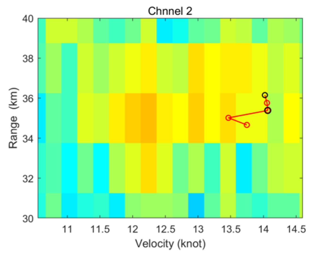
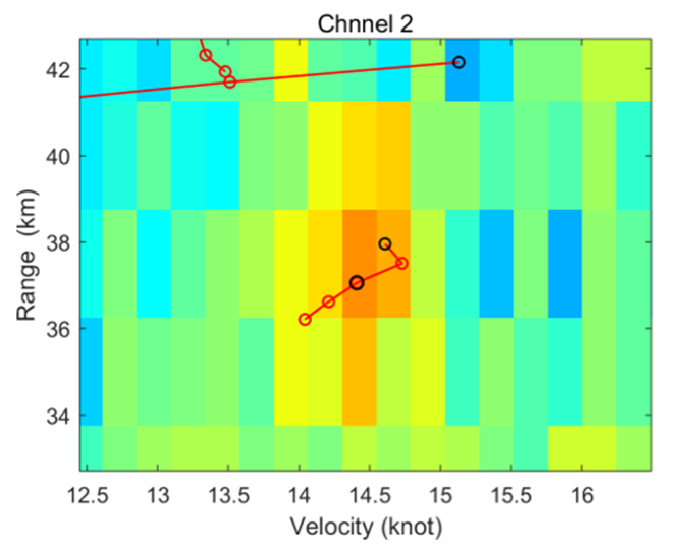
6.2. Interpretation of Experiment Results

In this paper, two targets in two different time periods are selected to analyze the target signals before and after motion compensation processing for the case of ship with non-uniform linear motion. During time period P1, during which the ship velocity changes greatly and the heading remains relatively stable. For time period P2, during which the ship heading changes greatly, the velocity remains relatively stable. Figure 26 shows the ship velocity and heading variations during P1 and P2.

During the time period P1, the ship heading remains relatively stable while the velocity changes greatly, which can be observed from Figure 26. During this period, the selected target T1 is 35km (its mmsi = 414,400,020) from the radar station, and the angle of the line from the ship target to the shipborne platform is 344° with respect to north. Figure 27 shows the corresponding RD spectrum (channel 2). In order to carry out comparative analysis and indirectly verify the effect of motion compensation, a period right before P1 during which the ship velocity and heading change little is selected. The corresponding target RD spectrum are shown in Figure 28.

During the period before P1, the ship velocity and heading are relatively stable (i.e., uniform linear motion). The velocity is 10 knots and the heading is about 322°. In this case, the target signal is more concentrated with a peak of value 207.9 dB, and it can be easily identified because of its high SNR. However, during the P1 period, the target signal was broadened because the shipborne platform velocity gradually decreased from 10 knots to 6.5 knots. At this time, the peak value of T1 is only 204.7 dB, which is 3.2 dB lower than that of the case with uniform linear motion, so the SNR is low and the target detection becomes difficult.

Figure 29 shows the echo spectra before and after motion compensation. It can be seen that the width of the vessel target signal is reduced from a span of nearly 4 knots to less than 1 knot after motion compensation. Meanwhile, the peak value of the target echo is increased from 204.7 dB to 207.2 dB, which is close to the peak value of 207.9 dB, while the ship was in uniform motion. As a result, the target echo can be easily detected.

For the case during the P2 period, both the ship heading and velocity changed. The heading changes from 333° to 296°, and the velocity also changed from 8.1 knots to 9.1 knots. The corresponding motion compensation results are shown in Figure 30. As can be seen for target T2, its peak value is increased from 213.9 dB to 214.7 dB after motion compensation, and the SNR is improved by 0.8 dB. Compared with the first case, although the broadening width of the second target is also reduced, the improvement of SNR is relatively little. According to the analysis in Section 5, motion compensation processing requires high heading accuracy. The reason for trivial improvement may be related to the heading error of the shipborne platform, which mainly depends on the measurement accuracy of the inertial navigation system.

7. Conclusions

In this paper, based on the target echo model for an HFSWR on a sailing ship, the Doppler shift of a moving target was derived. Next, the echo spectrum characteristics of a moving target under different ship motion conditions were investigated via simulation. The simulation results showed that the Doppler shift of the target signal not only depends on its own velocity but also the ship motion. The echo of the moving target only shows a frequency shift without broadening when the ship is in a uniform linear motion, while it will also be broadened if the ship undertakes non-uniform linear motion and yaw. The broadening of the target echo will lead to a reduction in SNR, which in turn may cause missed detection of a target. In addition, periodic changes in the velocity and yaw angle will cause false target echoes and negatively affect target detection. For this reason, motion compensation processing for the radar signal is important before target detection for shipborne HFSWR under non-uniform linear motion. Thus, a motion compensation scheme for improving the target echo was proposed, which involves heading compensation for yaw effect and velocity compensation in case of non-uniform ship movement. Based on the proposed method, motion compensation results under different non-uniform linear motions were compared. Moreover, the influence of the velocity and yaw angle measurement accuracy on the compensation results was analyzed. The analysis results showed that heading measurement with high accuracy should be used so that the SNR and target detection rate can be improved by using the motion compensation method proposed in this paper. Finally, the target echo characteristics and motion compensation method for shipborne HFSWR were verified by using the field experiment data. Experiment results showed that the broadening of target echoes caused by non-uniform ship motion can be significantly reduced and the SNR can be improved by about 2 dB after motion compensation.

In the future, quantitative analysis of the effectiveness of the proposed method in improving target detection and tracking performance using field data should be conducted. Moreover, it is necessary to verify whether the proposed motion compensation method is applicable to more complex situations. Furthermore, the influence of motion compensation on first-order sea clutter should also be investigated.

References

1. Ponsford, A.M. Surveillance of the 200 Nautical Mile Exclusive Economic Zone (EEZ) Using High Frequency Surface Wave Radar (HFSWR). Can. J. Remote. Sensing. 2001, 27, 354–360. [Google Scholar] [CrossRef]
2. Xie, J.; Yuan, Y.; Liu, Y. Experimental analysis of sea clutter in shipborne HFSWR. IEEE Proc. Radar Sonar Navig. 2001, 148, 67–71. [Google Scholar] [CrossRef]
3. Xie, J.; Yao, G.; Sun, M. Ocean Surface Wind Direction Inversion Using Shipborne High-Frequency Surface Wave Radar. IEEE Geosci. Remote. Sens. Lett. 2017, 14, 1283–1287. [Google Scholar] [CrossRef]
4. Chang, G.; Li, M.; Xie, J. Ocean Surface Current Measurement Using Shipborne HF Radar: Model and Analysis. IEEE J. Ocean. Eng. 2016, 41, 970–981. [Google Scholar] [CrossRef]
5. Sun, M.; Xie, J.; Ji, Z. Remote sensing of ocean surface wind direction with shipborne high frequency surface wave radar. In Proceedings of the 2015 IEEE Radar Conference (RadarCon), Arlington, VA, USA, 10–15 May 2015; pp. 0039–0044. [Google Scholar]
6. Walsh, J.; Huang, W.; Gill, E.W. The First-Order High Frequency Radar Ocean Surface Cross Section for an Antenna on a Floating Platform. IEEE Trans. Antennas Propag. 2010, 58, 2994–3003. [Google Scholar] [CrossRef]
7. Ma, Y.; Gill, E.W.; Huang, W. First-order bistatic high-frequency radar ocean surface cross-section for an antenna on a floating platform. IET Radar Sonar Navig. 2016, 10, 1136–1144. [Google Scholar] [CrossRef] [Green Version]
8. Ma, Y.; Gill, E.W.; Huang, W. Bistatic High-Frequency Radar Ocean Surface Cross Section Incorporating a Dual-Frequency Platform Motion Model. IEEE J. Ocean. Eng. 2018, 43, 205–210. [Google Scholar] [CrossRef]
9. Xie, J.; Sun, M.; Ji, Z. First-order ocean surface cross-section for shipborne HFSWR. Electron. Lett. 2013, 49, 1025–1026. [Google Scholar] [CrossRef]
10. Sun, M.; Xie, J.; Ji, Z. Ocean surface cross sections for shipborne HFSWR with sway motion. Radio Sci. 2017, 51, 1745–1757. [Google Scholar] [CrossRef] [Green Version]
11. Yao, G.; Xie, J.; Ji, Z. The first-order ocean surface cross section for shipborne HFSWR with rotation motion. In Proceedings of the 2017 IEEE Radar Conference (RadarConf), Seattle, WA, USA, 8–12 May 2017; pp. 0447–0450. [Google Scholar]
12. Yao, G.; Xie, J.; Huang, W. First-order ocean surface cross-section for shipborne HFSWR incorporating a horizontal oscillation motion model. IET Radar Sonar Navig. 2018, 12, 973–978. [Google Scholar] [CrossRef]
13. Ji, Y.; Zhang, J.; Wang, Y. Coast–Ship Bistatic HF Surface Wave Radar: Simulation Analysis and Experimental Verification. Remote. Sens. 2020, 12, 470. [Google Scholar] [CrossRef] [Green Version]
14. Gill, E.W.; Ma, Y.; Huang, W. Motion compensation for high-frequency surface wave radar on a floating platform. IET Radar Sonar Navig. 2018, 12, 37–45. [Google Scholar] [CrossRef]
15. Ma, Y.; Huang, W.; Gill, E.W. Motion compensation for platform-mounted high frequency surface wave radar. In Proceedings of the 2017 18th International Radar Symposium (IRS), Prague, Czech Republic, 28–30 June 2017. [Google Scholar]
16. Shahidi, R.; Gill, E.W. Time-Domain Motion Compensation of HF-Radar Doppler Spectra for an Antenna on a Moving Platform. In Proceedings of the 2019 IEEE/OES Twelfth Current, Waves and Turbulence Measurement, San Diego, CA, USA, 10–13 March 2019; pp. 1–4. [Google Scholar]
17. Zhu, D.; Niu, J.; Li, M. Motion Parameter Identification and Motion Compensation for Shipborne HFSWR by Using the Reference RF Signal Generated at the Shore. Remote. Sens. 2020, 12, 2807. [Google Scholar] [CrossRef]
18. Xie, J.; Yuan, Y.; Liu, Y. Suppression of sea clutter with orthogonal weighting for target detection in shipborne HFSWR. IEE Proc. Radar Sonar Navig. 2002, 149, 39–44. [Google Scholar] [CrossRef]
19. Ji, Z.; Duan, Z.; Xie, J. STAP process of shipborne HFSWR motion compensation. Int. Conf. Signal Process. 2012, 3, 1856–1860. [Google Scholar]
20. Ji, Z.; Yi, C.; Xie, J. The Application of JDL to Suppress Sea Clutter for Shipborne HFSWR. Int. J. Antennas Propag. 2015, 2015, 1–6. [Google Scholar] [CrossRef]
21. Yi, C.; Ji, Z.; Kirubarajan, T. An Improved Oblique Projection Method for Sea Clutter Suppression in Shipborne HFSWR. IEEE Geosci. Remote. Sens. Lett. 2016, 13, 1089–1093. [Google Scholar] [CrossRef]
22. Zhu, L.; Wei, Y.; Zhu, K. Sea clutter suppression for shipborne HFSWR using joint sparse recovery-based STAP. Electron. Lett. 2016, 52, 1067–1069. [Google Scholar] [CrossRef]
23. Skolnik, M.I. An Empirical Formula for the Radar Cross Section of Ships at Grazing Incidence. IEEE Trans. Aerosp. Electron. Syst. 1974, AES-10, 292. [Google Scholar] [CrossRef]
Figure 1. The diagram of the relative position of the moving target and shipborne platform.
Remotesensing 13 02826 g001
Figure 2. The physical model of shipborne HFSWR platform.
Remotesensing 13 02826 g002
Figure 3. The physical model of the shipborne HFSWR platform in case of heading changing during the navigation.
Remotesensing 13 02826 g003
Figure 4. Target echoes simulation results for shipborne HFSWR in the case of uniform linear platform motion: (a) channel results with and without noise, (b) channel results at different velocities, (c) beam results at angle 1, (d) beam results at angle 2.
Remotesensing 13 02826 g004
Figure 5. Simulation results of sea clutter spectrum in case of uniform linear motion: (a) channel results when the wind direction is 90°, (b) channel result when the wind direction is 180°, (c) beam results at angle 1 when the wind direction is 180°, (d) beam results at angle 2 when the wind direction is 180°.
Remotesensing 13 02826 g005
Figure 6. Simulation results of target echo in case of uniform deceleration linear motion: (a) the distribution of the velocity and heading of the platform, (b) channel result, (c) beam result at range1, (d) beam result at range2.
Remotesensing 13 02826 g006
Figure 7. Simulation results of target echo when the velocity of the platform varies periodically: (a) the distribution of the velocity and heading of the platform, (b) channel results, (c) beam result at range1, (d) beam result at range2.
Remotesensing 13 02826 g007
Figure 8. Simulation results of target echo in case of uniform variation of heading when velocity is 10 knots: (a) the distribution of the velocity and heading of the platform, (b) channel results, (c) beam results at range1, (d) beam results at range2.
Remotesensing 13 02826 g008
Figure 9. Simulation results when the yaw angle varies periodically: (a) the distribution of the velocity and heading of the platform, (b) channel results when Vp = 0 knot, (c) beam simulation result of target 1 when Vp = 0 knot, (d) beam simulation result of target 1 when Vp = 10 knot.
Remotesensing 13 02826 g009
Figure 10. Simulation results when both heading and velocity of ship change: (a) the distribution of the velocity and heading of the platform, (b) beam results of target 1 at angle1, (c) beam results of target 2 at angle2.
Remotesensing 13 02826 g010
Figure 11. Flow chart of motion compensation for shipborne HFSWR.
Remotesensing 13 02826 g011
Figure 12. Compensation result for the case of uniform deceleration motion: (a) compensation result for angle1, (b) compensation result for angle2.
Remotesensing 13 02826 g012
Figure 13. Space–time two-dimensional spectrum before and after motion compensation for case of uniform deceleration motion: (a) results before motion compensation, (b) results after motion compensation.
Remotesensing 13 02826 g013
Figure 14. Compensation result for the case of uniform yaw motion: (a) when ship velocity is 5 knots, (b) when ship velocity is 15 knots, (c) when ship velocity is 15 knots.
Remotesensing 13 02826 g014aRemotesensing 13 02826 g014b
Figure 15. Space–time two-dimensional spectrum before and after motion compensation for the case of uniform yaw motion when ship velocity is 10 knots: (a) results before motion compensation, (b) results after motion compensation.
Remotesensing 13 02826 g015
Figure 16. Compensation result for case of uniform deceleration motion: (a) compensation result for angle1, (b) compensation result for angle2.
Remotesensing 13 02826 g016
Figure 17. Space–time two-dimensional spectrum before and after motion compensation when ship velocity is 10 knots; the swing period P = 20 s and the swing amplitude is 5°: (a) results before motion compensation, (b) results after motion compensation.
Remotesensing 13 02826 g017
Figure 18. Compensation result for case of uniform deceleration motion: (a) compensation result for angle1, (b) compensation result for angle2, (c) zoom in of peak for target 1, (d) zoom in of peak for target 2.
Remotesensing 13 02826 g018
Figure 19. Space–time two-dimensional spectrum before and after motion compensation when both velocity and heading change: (a) results before motion compensation, (b) results after motion compensation.
Remotesensing 13 02826 g019
Figure 20. Motion compensation results under different velocity measurement errors: (a) compensation result for angle1, (b) compensation result for angle2.
Remotesensing 13 02826 g020
Figure 21. Statistical table of the SNR for the two targets before and after motion compensation under different velocity errors: (a) target 1, (b) target 2.
Remotesensing 13 02826 g021
Figure 22. Motion compensation results under different heading measurement error: (a) compensation result for angle1, (b) compensation result for angle2.
Remotesensing 13 02826 g022
Figure 23. Statistical table of the SNR for the two targets before and after motion compensation under different heading measurement errors: (a) target 1, (b) target 2.
Remotesensing 13 02826 g023
Figure 24. Location of coast-based radar station and navigation route of the ship.
Remotesensing 13 02826 g024
Figure 25. Velocity and heading of the ship.
Remotesensing 13 02826 g025
Figure 26. The variation of the ship velocity and heading: (a) during P1, (b) during P2.
Remotesensing 13 02826 g026
Figure 27. RD images of T1 during P1.
Remotesensing 13 02826 g027
Figure 28. RD images of T1 during the period with uniform linear motion before P1.
Remotesensing 13 02826 g028
Figure 29. Target T1 Doppler spectral results before and after motion compensation during P1: (a) two-dimensional RD spectral results before motion compensation, (b) two-dimensional RD spectral results after motion compensation, and (c) one-dimensional spectral results before and after motion compensation.
Remotesensing 13 02826 g029
Figure 30. Target T2 Doppler spectral results before and after motion compensation during P2: (a) two-dimensional RD spectral results before motion compensation, (b) two-dimensional RD spectral results after motion compensation, and (c) one-dimensional spectral results before and after motion compensation.
Remotesensing 13 02826 g030
Publisher’s Note: MDPI stays neutral with regard to jurisdictional claims in published maps and institutional affiliations.