Article

Characterizing the Relationship between the Sediment Grain Size and the Shoreline Variability Defined from Sentinel-2 Derived Shorelines

by
Carlos Cabezas-Rabadán
*,
Josep E. Pardo-Pascual
and
Jesus Palomar-Vázquez
Geo-Environmental Cartography and Remote Sensing Group (CGAT-UPV), Department of Cartographic Engineering, Geodesy and Photogrammetry, Universitat Politècnica de València, Camí de Vera s/n, 46022 València, Spain
*
Author to whom correspondence should be addressed.
Remote Sens. 2021, 13(14), 2829; https://0-doi-org.brum.beds.ac.uk/10.3390/rs13142829
Submission received: 9 June 2021 / Revised: 1 July 2021 / Accepted: 15 July 2021 / Published: 19 July 2021
(This article belongs to the Special Issue Satellite Mapping and Monitoring of the Coastal Zone)

Abstract

:
Sediment grain size is a fundamental parameter conditioning beach-face morphology and shoreline changes. From remote sensing data, an efficient definition of the shoreline position as the water–land interface may allow studying the geomorphological characteristics of the beaches. In this work, shoreline variability is defined by extracting a set of Satellite Derived Shorelines (SDS) covering about three and a half years. SDS are defined from Sentinel 2 imagery with high accuracy (about 3 m RMSE) using SHOREX. The variability is related to a large dataset of grain-size samples from the micro-tidal beaches at the Gulf of Valencia (Western Mediterranean). Both parameters present an inverse and non-linear relationship probably controlled by the beach-face slope. High shoreline variability appears associated with fine sands, followed by a rapid decrease (shifting point about medium/coarse sand) and subsequent small depletions as grain sizes increases. The relationship between both parameters is accurately described by a numerical function (R2 about 0.70) when considering samples at 137 open beaches. The definition of the variability is addressed employing different proxies, coastal segment lengths, and quantity of SDS under diverse oceanographic conditions, allowing to examine the effect they have on the relation with the sediment size. The relationship explored in this work improves the understanding of the mutual connection between sediment size, beach-face slope, and shoreline variability, and it may set up the basis for a rough estimation of sediment grain size from satellite optical imagery.

Graphical Abstract

1. Introduction

Beaches are highly dynamic and changing natural environments that provide protection to the coast, habitat for unique species and constitute a basic recreational resource for coastal societies. Given the importance of these functions, it is a primary goal to define the state of the beaches and understand their behavior so as to improve their management. Sediment size and slope are key geomorphological elements for characterizing the beaches as they appear interrelated with each other and with the oceanographic conditions [1,2,3]. These geomorphological aspects condition beach functions by defining the abundance of biota [4], beachgoers perception [5] and safety [6], and beach response to stress factors as storms [7,8,9].
Due to the important role grain size plays its characterization is fundamental for decision-making and planning, as well as for forecasting purposes through modeling. However, the insufficient detailed data usually leads to oversimplifications of the grain-size distribution hampering advances in coastal modeling [10]. The quantification of sediment grain size by traditional techniques is a time-consuming task that hinders the collection of repetitive data over long coastal segments. They require in-situ sampling together with the subsequent characterization in the laboratory by sieving or the use of laser particle-sizer. Different methods have been proposed to reduce the costs of data obtention. At the microscale level, photogrammetric techniques allow quantifying the grain size (e.g., [10,11,12,13,14,15]) applying processing algorithms over images. Trying to reach a larger coverage, a terrestrial laser scanner (TLS) has been repeatedly employed for modeling river bed roughness and estimating surface sedimentology (e.g., [16,17]). Different approaches have appeared sustained in the use of unmanned aerial vehicles (UAV) (e.g., [18,19,20,21,22]) although comparisons between studies and validations are scarce, and only the highest image resolutions seem to offer acceptable results for quantifying finer grains [18]. Due to the important field and processing efforts those techniques require, any of them constitutes a valid option for estimating grain size along large territories. In order to increase the spatial coverage, airborne solutions (e.g., [23,24]) and satellite images have been proposed to obtain macroscale information. The characterization of soil properties and the mapping of the distribution of intertidal surface sediments have been addressed from mid-resolution imagery (e.g., [25]), synthetic-aperture radar (e.g., [26,27,28]), and their combination (e.g., [29,30]). However, those techniques are constrained by the coarse resolution of the images. Taking all this into account, and despite the rapid development of remote sensing methodologies, no single technique is capable of carrying out an efficient quantification of the grain size at the mesoscale level. While some of them maintain the need for intensive fieldwork tasks, others only lead to a rough classification of the sediment.
Many studies have analyzed the relationship between sediment grain size, beach morphology, and slope along the profile (e.g., [31,32,33,34,35]). Grain size is a major factor defining the slope [1,32] as coarser grains are associated with higher infiltration and lower backwash transport of sediment, leading to higher slopes [36,37]. Different numerical models have been formulated to describe slope as a function of the grain size (e.g., [38,39,40]), most of the times employing linear equations adjusted by measurements on sandy beaches. In a recent work, Bujan et al. [41] compiled from literature a large number of grain size and slope measurements. Even though the high scattering of the data the meta-analysis evidenced that the relation between both parameters does not follow a simple trend. The data distribution was fitted with a non-linear function that starts with gentle slopes associated with fine sand grains, experiences a steep increase as sediment size grows, and around medium/coarse sand it shifts and becomes gentle for coarser sands, gravels and boulders.
The shoreline position is a representative feature of the morphology of the beach and is useful for describing its behavior [42]. Thus, the mobility of a beach, defined by Dolan et al. [43] as the standard deviation of the mean shoreline position, was related to the morphodynamic state of the beach [44]. Numerous works have quantified shoreline changes to characterize beach dynamics, understand their nature, and forecast its changes. Many of the recent works in coastal changes have defined the shoreline by fieldwork (e.g., [45,46,47,48,49]), limiting the spatial and/or temporal extension of the work. Recent remote sensing methodologies allow defining the position of the shoreline from freely available mid-resolution satellite imagery using subpixel extraction algorithms (e.g., [50,51,52]). SHOREX system [53] allows to efficiently extract Satellite Derived Shorelines (SDS) at regional scale from Sentinel-2 imagery offering accuracy levels of similar magnitude than video monitoring at different types of coast [54,55]. SDS obtained with this methodology have been proved to be useful to characterize the width of the beaches and its sub-annual changes [56], even of limited magnitude [57,58]. For the moment, SDS have barely been used to obtain information about other geomorphological aspects of the beach. Only very recently, Vos et al. [59] have dealt with the relation between shoreline changes and beach-face slope by estimating the latter one from SDS by frequency domain analysis. Considering the forehead stated relationship between grain size and beach-face slope, beaches with coarser material and steeper slopes are expected to show lower shoreline variabilities. This is due to the fact that water-level changes (either cyclical or punctual) will be translated into different horizontal displacements of the shoreline greatly depending on the beach-face slope.
The capacity to efficiently define shoreline variability from SDS may be helpful for exploring the interrelations between sediment size, beach-face slope, and shoreline changes. Establishing this relationship may set up the basis for a rough characterization of sediment size along large beach segments from a freely available source of data. Taking this into account, the main goal of this work is to characterize the relationship between sediment size and shoreline variability determined from multiple Sentinel-2 derived shorelines. The study aims (i) to propose a numerical description of the relation, (ii) to examine how oceanographic conditions, amount of SDS, and employed proxies condition the quantification of the variability, and (iii) to assess the potential for estimating sediment grain size from shoreline variability.

2. Materials and Methods

The work is mainly supported by two data sets available at the same study sites: on the one hand, satellite-derived shorelines used to quantify the shoreline variability and, on the other hand, sediment grain size data.

2.1. Study Area

The study took place along the beaches of the Gulf of Valencia (Eastern Spain, Iberian Peninsula), a coastal segment approximately 200 km long between the Ebro Delta and the Girona river mouth (Figure 1). It is a sedimentary coast mainly composed of medium and fine sandy beaches together with some gravel and pebbly ones [60,61]. Beaches face SE in the northern half of the Gulf, and NE in its southern half.
The coast has an average astronomical tidal range below 20 cm with small waves (mean annual values of Hs = 0.7 m; Tp = 4.2 s; Figure 2). It is a low-energy environment, although during storms waves may reach significant heights of 6.55 m and 15 s of peak period, mainly from NE-E, and sea level may increase by 1.32 cm [60]. The distribution of the sediment along the region was previously conditioned by a strong southerly littoral drift. This is a coast where the sediment does not show significant changes compared to the records of decades ago [61]. Nevertheless, this natural regime is punctually altered by many hard structures as ports and groins. They form a chain of artificial sediment traps that prevent the free distribution of the sediment [60]. Along with these constructions, numerous nourishment projects have been carried out during the last decades [62,63] in an attempt to maintain their width and carrying capacity. The southern end of the Gulf of Valencia has not been considered in the work because, on the one hand, there is no consistent information available on the repeated anthropogenic actions carried out in that sector and, on the other hand, the existence of submerged rocky formations condition shoreline mobility in a very different way from the rest of the beaches.
For this work, a total of 193 study sites were defined matching pre-existent sediment sampling locations. They appear distributed alongshore about every 500 m, although individual sites were expressly defined for shorter beach segments. Coastal formations other than beaches were discarded from the work. Similarly, segments in which shoreline mobility is conditioned by processes originated landwards (stream mouths) or by human interventions (nourishments carried out by the Ministry of the Environment’s Directorate General of Coasts) were discarded.
Landforms and offshore obstacles define the coastal shape and may condition shoreline mobility. In order to analyze their influence on the behavior of the shore, the study sites considered in the analysis were classified as follows (Figure 3):
-
Open beaches (137 sites): those in which sediment moves freely, without significant elements that could influence wave conditions. They are exposed to waves from NE, E, and SE.
-
Enclosed beaches (56 sites): those in which incident waves clearly differ from those recorded along the study area. This group includes beaches enclosed due to nearby coastal engineering structures as jetties, groins, and exempt dikes, as well as small natural pocket beaches.

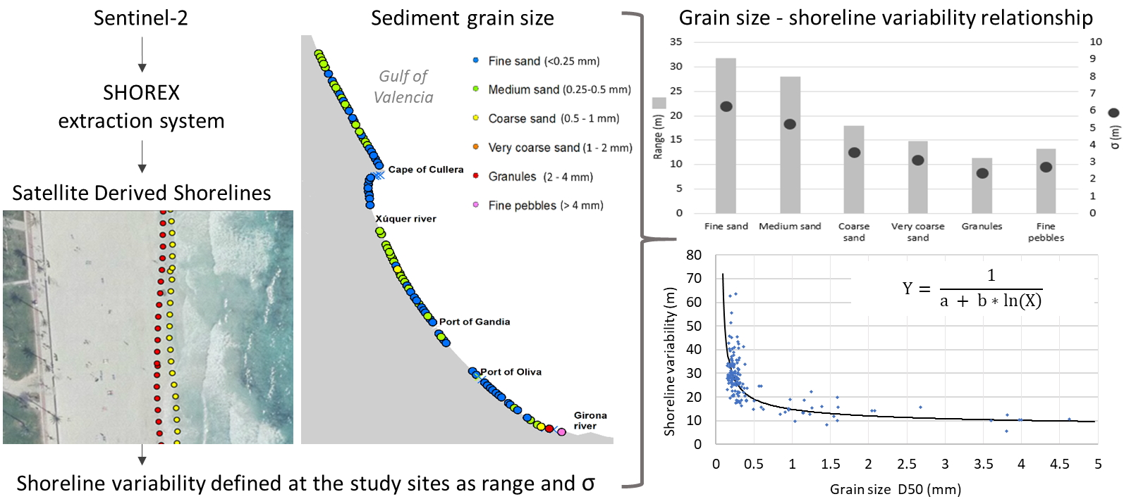
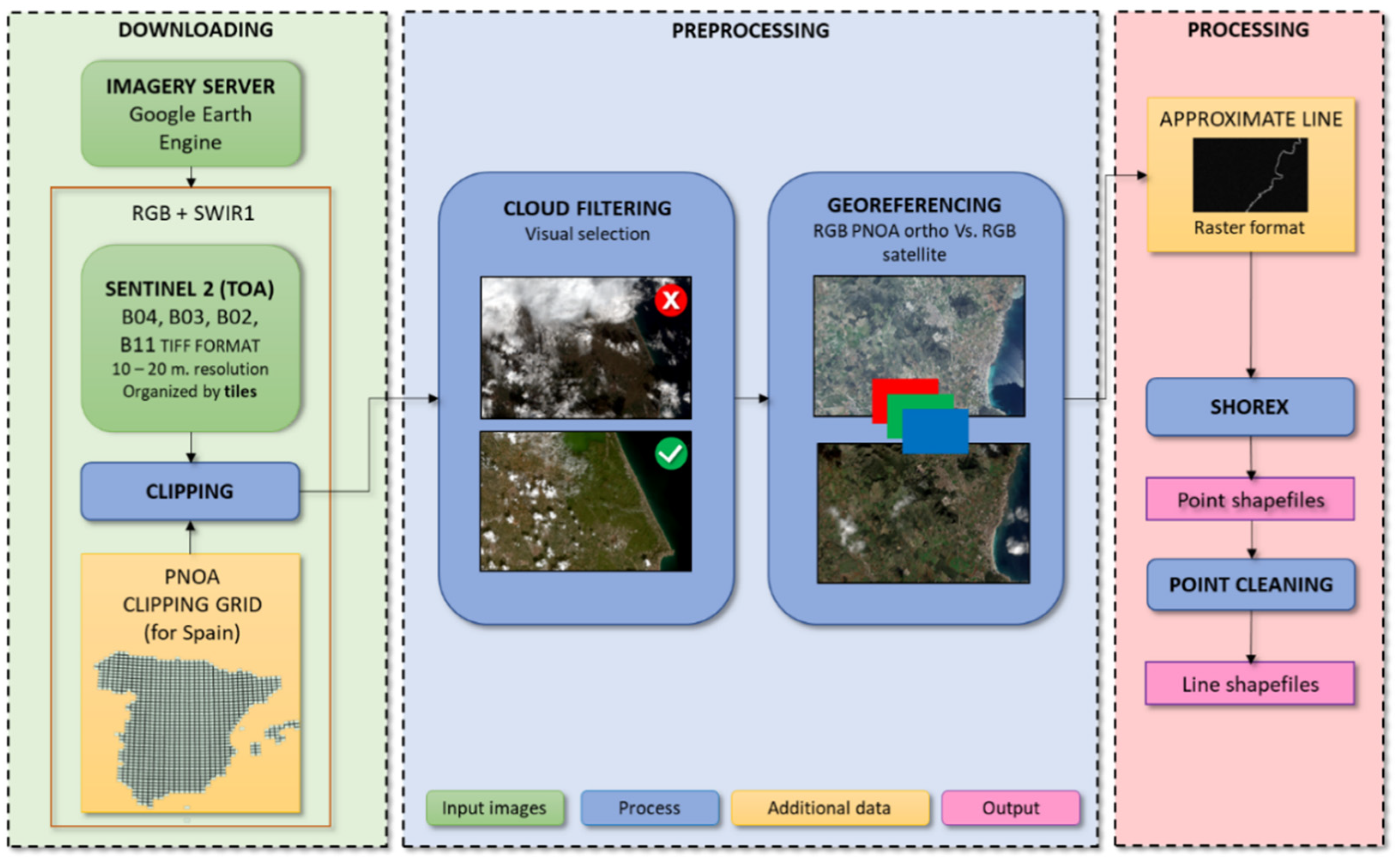
2.2. Satellite Derived Shorelines

Shoreline position was defined along the beaches of the Gulf of Valencia from Sentinel-2 Level-1C MSI imagery from July 2015 (starting with the first image acquired by the satellite) to January 2019 (Figure 2). According to previous assessments at similar micro-tidal beaches [54] the resulting SDS defines the water/land intersection at the instant each image is acquired with an estimated accuracy of 3.01 m RMSE.
For this work, the definition of the SDS was carried out using the software SHOREX. It is a system that includes as its core the algorithmic solution for the shoreline extraction with sub-pixel precision proposed by Pardo-Pascual et al. [64] and Almonacid-Caballer [65]. A set of separated tools have been progressively developed surrounding it. They are integrated within a single Python framework (see the preliminary version of the software described in Palomar-Vázquez et al. [53] defining a workflow that includes all the necessary operations to efficiently manage a large volume of satellite images (Figure 4).
The workflow starts with the downloading phase, in which Sentinel-2 RGB and SWIR1 bands are retrieved free of charge from Google Earth Engine (GEE) servers. To optimize the efficiency of the system, the original S2 tiles are clipped automatically into the GEE server and downloaded in TIFF format, according to the Spanish National Plan of Aerial Orthophotography (PNOA) grid. During the second phase of the workflow, the pre-processing, several actions are carried out. For this study, after discarding those images affected by major cloud coverage (automatic discard of those with more than 70% of clouds followed by a manual check of the beaches), 95 images/dates were considered for the study. This phase also includes the sub-pixel georeferencing following the method proposed by Guizar-Sicairos et al. [66] and modified to work as phase-correlation by Almonacid-Caballer et al. [67]. Finally, the processing consists of the shoreline extraction at the sub-pixel level. As the regional setting is a micro-tidal coast and the whole analysis period is relatively short, the extraction was automatically carried out from the pre-processed bands with the help of an initial approximate shoreline in raster format obtained from the Spanish National Geographic Institute (IGN) as described in Sánchez-García et al. [54]. This allowed to reduce the processing time and made manual thresholding processes no longer necessary. The extraction algorithm is applied along beach stretches, excluding artificial structures and natural rigid coastal segments. It operates over the Short-Wave Infrared bands (SWIR1) using a third-degree polynomial and 3 × 3 analysis kernel (60 m at S2 imagery). Thus, the extraction works optimally on relatively straight coasts, with an increasing error in areas adjacent to elements that cause abrupt changes in the orientation of the shore. For this reason, extremely short beach segments (tens of meters long) delimited by rigid structures (e.g., breakwaters and jetties) were discarded.

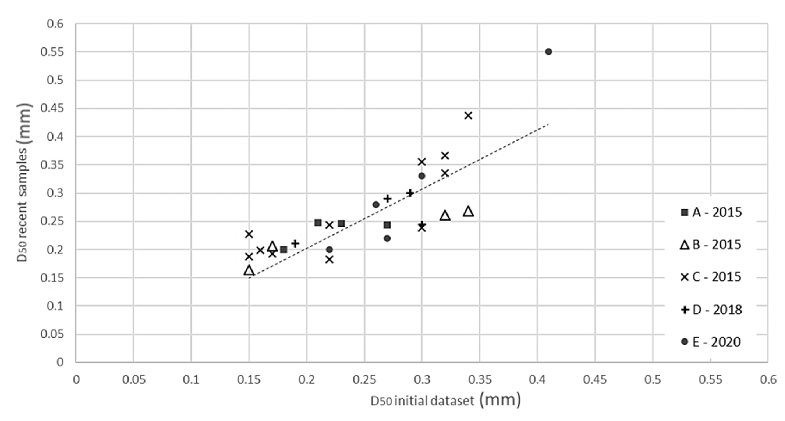
2.3. Sediment Grain size

The information regarding sediment size was obtained from a public database of the Spanish Ministry of Environment (ECOLEVANTE [68], available at https://www.miteco.gob.es/es/costas (accessed on 8 June 2021). Sampling locations were distributed along the beach segments of the Gulf of Valencia about every 500 m. Samples were acquired using a Van Veen grab sampler through 2006–2007 (center and southern sectors of the study area respectively) and 2010 (northern sector). The grain size was characterized by sieving 100 g of sediment using a nested column of 13 mesh strainers from 64 mm to 0.063 mm. It allowed defining the median grain diameter (D50) according to Folk & Ward parameters [69] allowing their classification in grades [70]. The study focuses on the beach-face samples at 0 m MSL as the sediment at that point is considered to be closely related to shoreline behavior.
It is important to underline that sediment samples and SDS are not synchronous in time. In order to address this issue, a second and smaller dataset has been defined from five sampling campaigns. A total of 28 more recent (between years 2015 and 2020) and spatially-coincident samples have been compared with those composing the initial sediment dataset (Figure 5). The pairs of data show a linear fit (slope about 1) with both populations following an identical pattern. While 24 of the new samples (86%) maintained the original grades, 4 changed their classification shifting to an adjacent grade, leading to an average difference of D50 of 15%. Thus, changes in grain size that occurred between the sediment dataset and SDS definition can be considered to be of moderate magnitude, validating the use of the first granulometric dataset.

2.4. Quantifying Shoreline Variability and Its Relation with Grain Size

Grain-size data were paired with the temporal variability of the shoreline position at each study site. The variability along time was quantified with GIS software from the SDS following the methodology described by Cabezas-Rabadán et al. [56,57]. In order to do so, the inner limit of the beach (e.g., promenades, buildings and dune toes) was defined by photointerpretation of orthophotography. That inner limit was considered as a constant baseline from which the distance to the points that compose each SDS were measured (Figure 6), constituting beach widths. For each study site and date, the average beach width was defined, constituting a relative position of the shoreline.
Three parameters were combined to define the temporal variability of the shoreline position:
(i)
Shoreline segment’s length. Two different shoreline lengths were employed at each study site for defining the variability in order to compare the effect of relatively small morphological formations (e.g., beach megacusps). Thus, the segments of SDS employed in the analysis were selected using 100 and 200 m buffers around the sediment samples.
(ii)
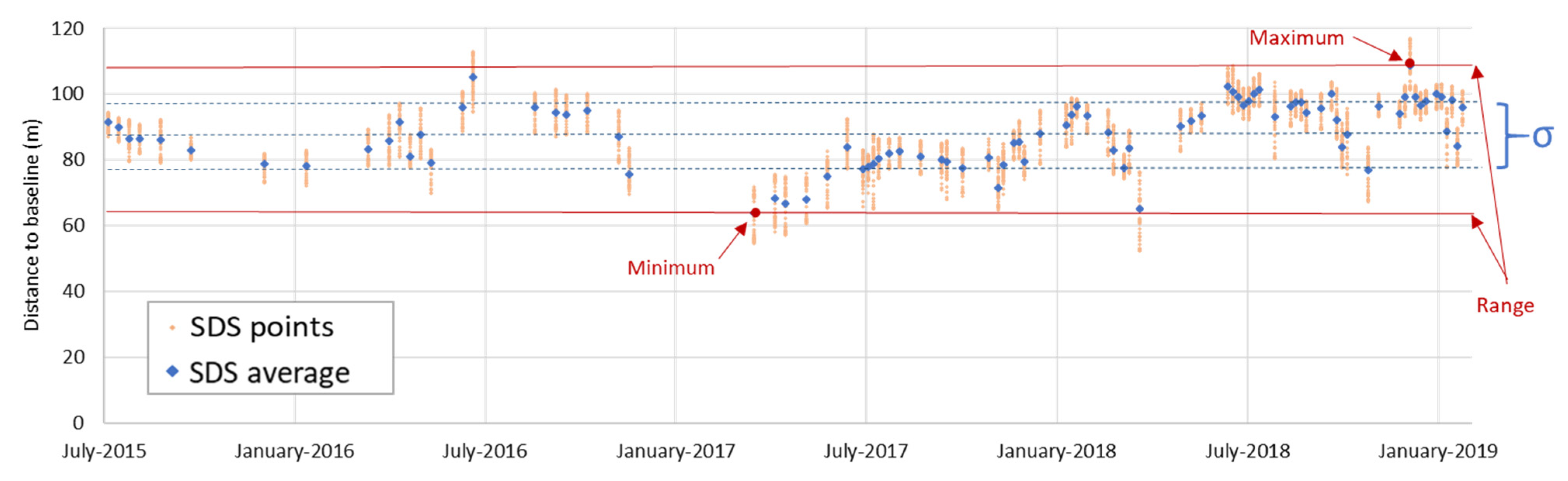
Variability proxy. In order to quantify the shoreline variability, the standard deviation (hereafter σ) and the maximum range were defined considering the average SDS position on different dates (Figure 6). The standard deviation has been stated by previous works as representative of beach variability (e.g., [43,44,48,74]), while the range is directly related to the maximum changes that the total water level (TWL) and beach-face morphology experience.
(iii)
Period and quantity of SDS. The intra-annual variability was defined considering the corresponding SDS and using the previously described proxies and segments of analysis. This allowed analysis of the influence of the number of SDS considered as well as the associated oceanographic conditions.
Subsequently, shoreline variability was defined at each study site through the combination of different proxies, lengths of shoreline segments, and periods of time. Variability values were paired with grain-size data from the most recent dataset available. Different numerical functions were tested to describe the shape of the distribution across the full grain-size spectrum. The goodness of fit of the optimal model was compared when combining different parameters for defining the variability.

3. Results

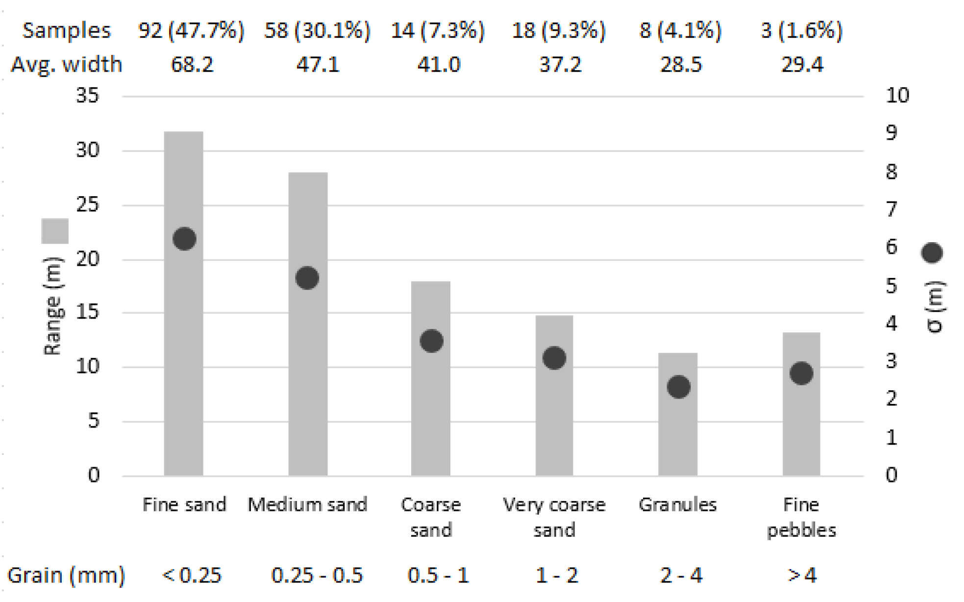
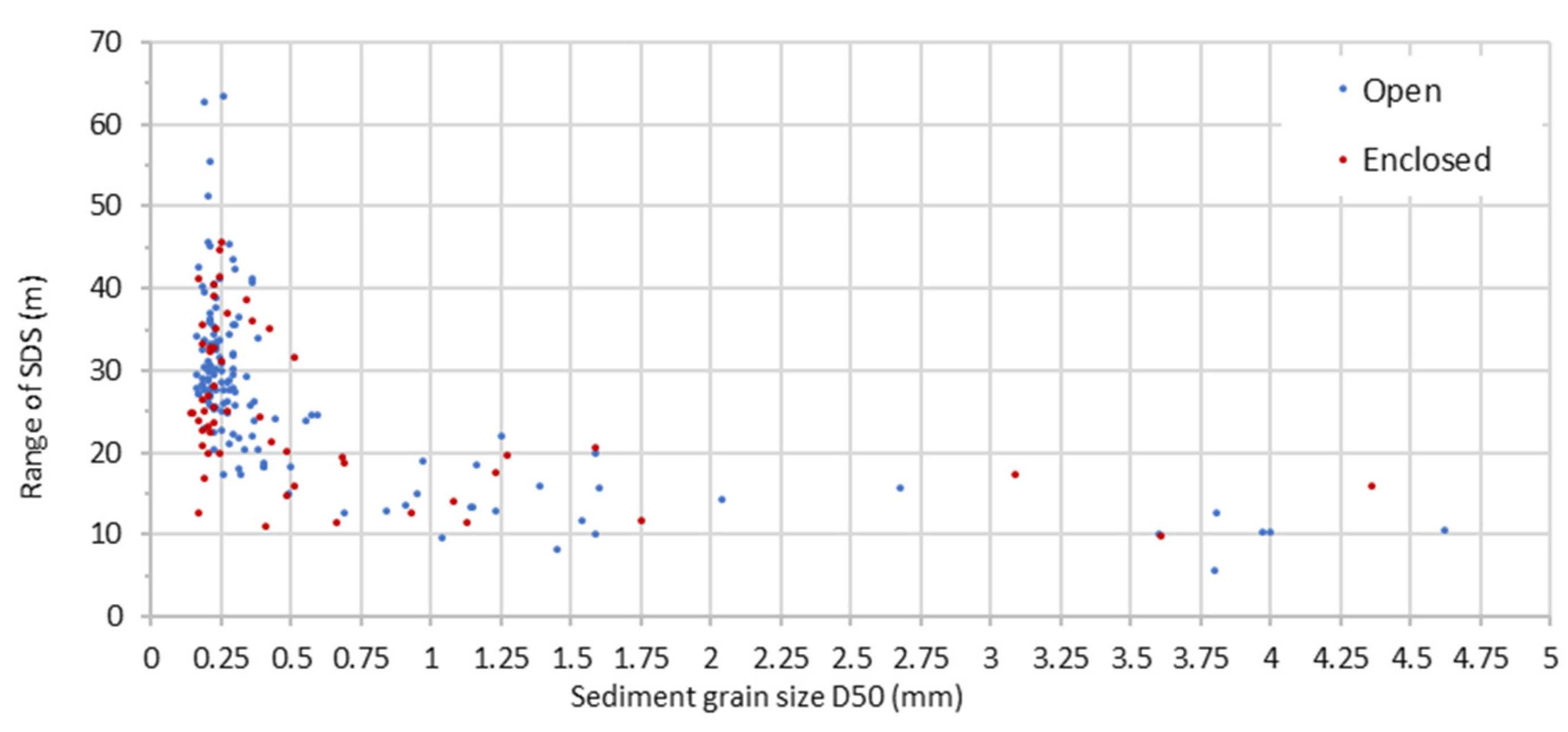
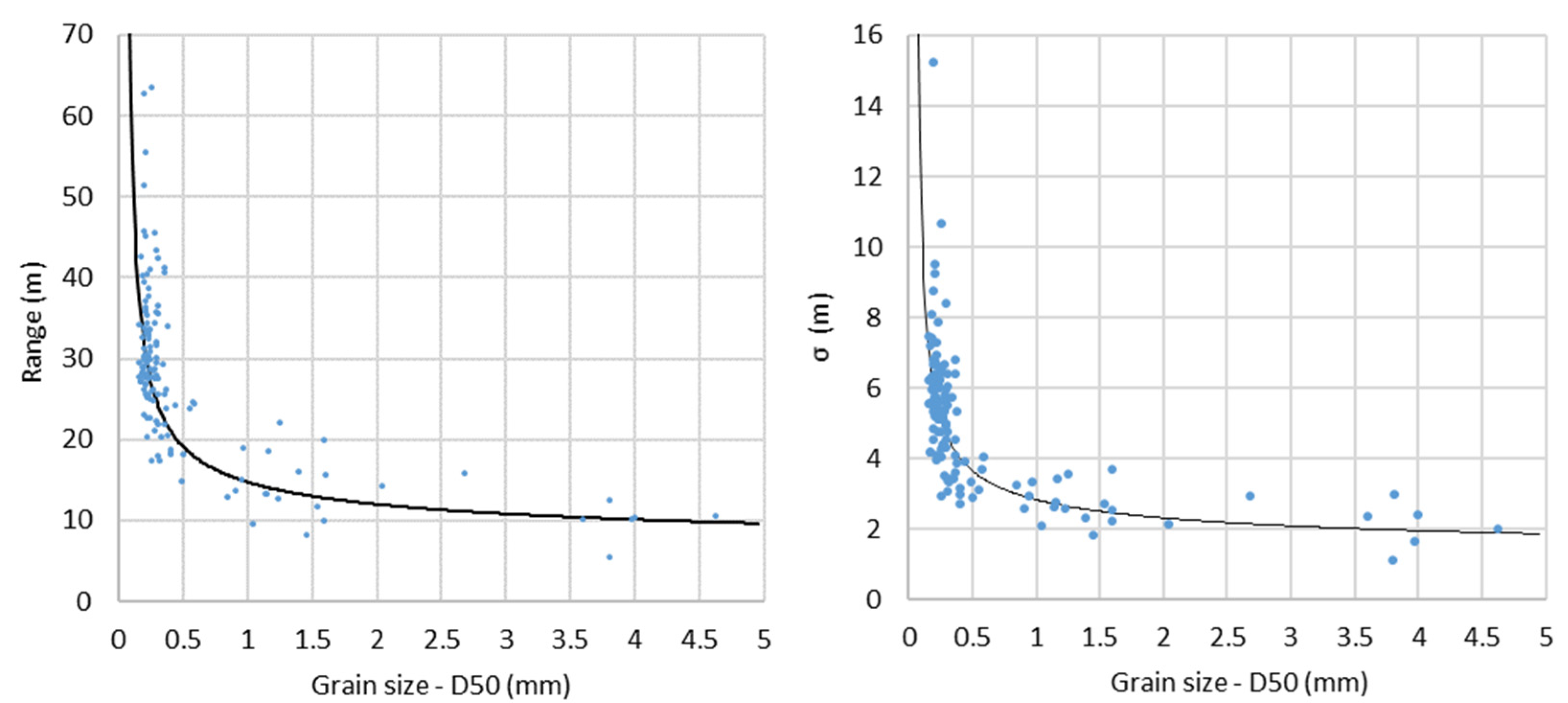
3.1. Grain Size and Shoreline Variability Data Pattern

Shoreline variability was defined based on different proxies. The average values of the variability proxies were obtained for the different sediment-size categories (Figure 7).
Throughout the sediment size spectrum there is an evident gradation in the number of samples analyzed, values of shoreline variability, and beach width, all of them decreasing as grain size increases. Regarding the availability of samples (193) there is a significant imbalance along the grain-size spectrum. A greater quantity of samples (47.7%) appear associated with fine sand (being the smallest sample of D50 = 0.14 mm). The availability of samples decreases progressively through medium sand (30.1%), coarse (7.3%) and very coarse sand (9.3%), granules (4.1%), and fine pebbles (only 1.6%, being 4.66 mm the coarsest sample size). Concerning beach width, fine sand samples appear linked with wider beach segments (average width over 65 m) while granules and fine pebbles are associated with much narrower beaches (almost 30 m in both cases). Shoreline variability, defined by range and standard deviation proxies, presents a gradient with the highest values associated with fine sand (average range of 31.8 m and σ of 6.3 m) and decreasing towards granules and fine pebbles, showing both similar variabilities (range and σ about 12 m and 2.5 m respectively).
When considering each sample in combination with the associated shoreline variability the data present a remarkable scattering, although their distribution shows a clear pattern in which both parameters present an inverse and non-linear relationship (Figure 8). The scattering is especially remarkable for fine and medium sand samples, which show range values between 11 m and 63.5 m. The scattering and the variability decrease towards coarser sediments with an inflection in this trend about the medium and coarse sand categories. From this point, samples continue to show similar minimum ranges near 10 m, while most of the highest range values remain below 20 m. This reduction is maintained throughout the rest of the spectrum, with no samples of granules or pebbles showing range values greater than 20 m.
With regard to the morphology of the beaches, the general pattern of those enclosed is similar to the open ones. Nevertheless, several samples at enclosed beaches showed greater scattering from the general pattern. As they may experience different wave incidence and in order to be more consistent it was decided to not consider them when establishing the numerical grain size–variability relationship. Thus, subsequent analyses have been carried out only considering open beaches (137 study sites).

3.2. Numerical Description of the Relationship

Different numerical models were tested to describe the data pattern registered across the full range of grain sizes considering sediment samples of open beaches. The equation with two terms that best describes the relationship between grain size as a function of shoreline variability data has been defined as follows:
Y = 1 a   +   b ln ( X )  
where Y is the shoreline variability, and X the sediment grain size. The deduced logarithmic function describes the inverse and non-linear relationship between both parameters (Figure 8). The model represents high values of shoreline variability associated with fine sand followed by a rapid decrease and, subsequently, very small depletions as sediment size continues to increase. The turning point is linked to D50 values close to 0.5 mm.
The function offers a moderately-high agreement, explaining about 70% of the shoreline variability as a function of grain size. The goodness of fit of the model was compared when defining the variability by combining different variability proxies and coastal segment lengths (Table 1). Similar results are obtained when employing σ or range as proxies of shoreline variability. The same applies when defining the length of the segments of analysis with 100 m or 200 m buffers around sediment samples. In particular, the best results are achieved by logarithmic functions (Figure 9) using the σ as variability proxy over coastal lengths defined by 200 m buffers (R2 = 0.69), although it is a very close correlation to the one obtained when using the range and 100 m buffers (R2 = 0.68).

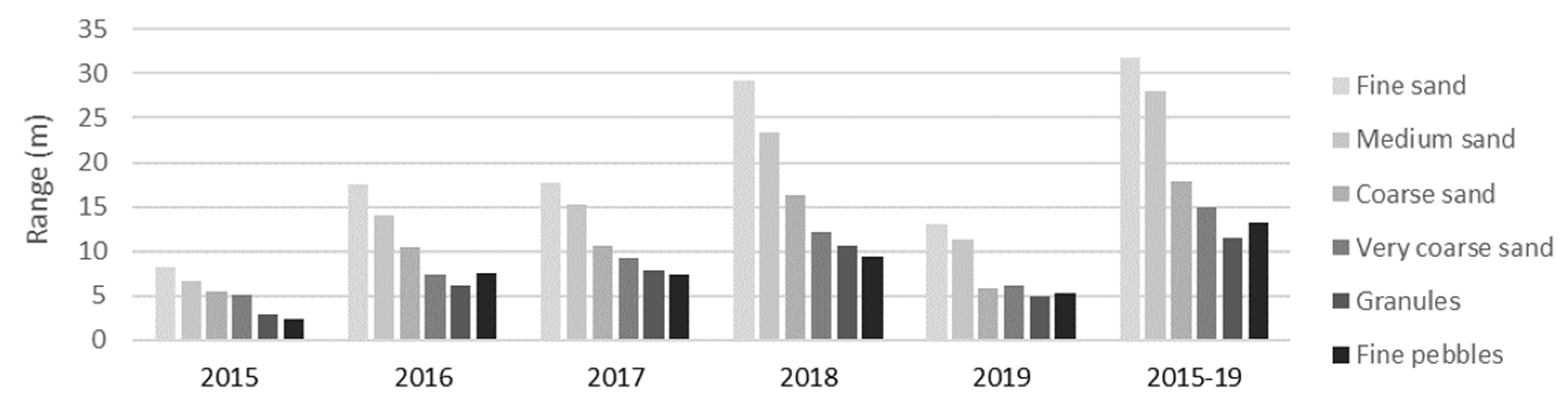
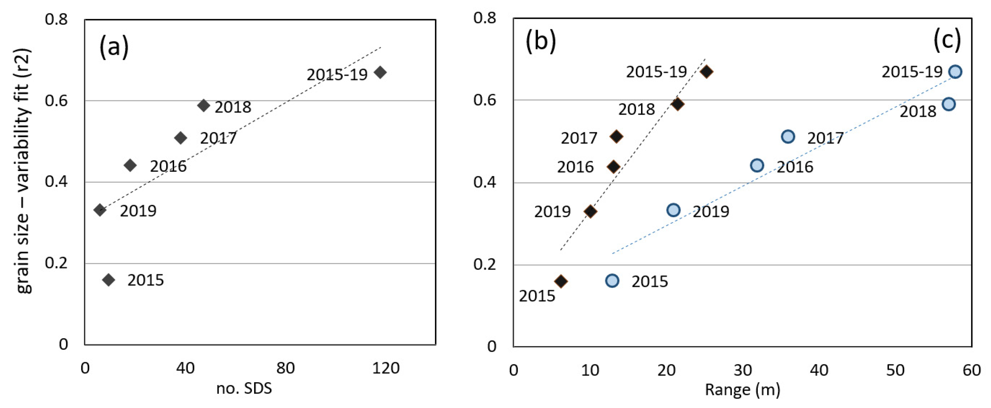
3.3. Annual Variability, Amount of SDS and Oceanographic Conditions

Shoreline variability experiences significant changes over the years (Figure 10). Expressed as average range, the variability shows a higher value for the period 2015-2019 (27 m) than when individually considering the different years. The year 2018 is the one with the largest average range (24 m), followed by 2016 (14.5 m) and 2017 (15.2 m). In contrast, 2015 and 2019 present substantially lower variability (7 m and 11 m respectively).
The distribution of variability with regard to different sediment sizes also experiences changes during the different years. In general, there is a gradation of variability from the finest to the coarsest sediment. Thus, during the period 2015–2019 the average range decreases progressively from fine sand (31.8 m) to granules and fine pebbles, that register an average range below half of it (11.4 m and 13.3 m). The distribution is very similar in 2018 and, although the variability values are reduced, the gradient is maintained for the rest of the years.
The goodness of fit of the model describing the shoreline variability as a function of the grain size was analyzed when defining the variability annually instead of for the whole period. The highest goodness of fit is obtained considering the period 2015–2019 (i.e., with the whole set of SDS), and it is lower when only SDS of a single year are considered (Table 2). Nevertheless, there are important differences between the years. The highest goodness of fit for a single year appears in 2018, the year with the highest availability of SDS. It is followed by 2017 and 2016 both by fit values and amount of available SDS, while 2015 and 2019 have much fewer SDS and offer much worse fit values. With regard to the proxies and lengths of coastal segments, the fit is similar for any combination of them as it occurs for the period 2015–2019.
A higher amount of SDS when defining the shoreline variability appears associated with higher goodness of the fit grain size–shoreline variability (Figure 11a), although this trend is not very strong and is sustained by a low amount of data. The figure also points out that the amount of SDS does not increase linearly the ability of their derived variability to deduce grain size. The goodness of fit only improves about 10% when using 118 SDS (period 2015–2019) instead of only 47 SDS. Moreover, important differences appear when comparing the two years with limited SDS availability. It is noteworthy that 2019 with only 6 SDS registers substantially better goodness of fit than 2015 with 9 SDS, suggesting that the amount of SDS is not the only relevant factor. Thus, for a certain period the goodness of the grain size–variability fit appears also linked to the recorded magnitude of shoreline change (Figure 11b). Higher shoreline variability values, expressed by the proxy annual range, appear linked to higher goodness of fit with sediment size. This relationship (R2 = 0.89) is stronger than that one registered with the amount of SDS used to define the shoreline variability, as it can be seen by comparing Figure 11a,b scatter plots.
The magnitude of shoreline variability seems to play a major role in the fit of this parameter with grain size. As shoreline changes are conditioned by sea level, its annual influence on SDS position was also explored. Sea level data at the time of acquisition of each SDS were identified and their annual range was calculated. They were compared with the annual goodness of grain size–variability fit, showing a clear linear relationship (R2 = 0.93) between both variables (Figure 11c). In line with that, considering the SDS acquired during the period 2015–2019 those associated with the highest and lowest sea levels were selected (almost 25% for each case, a total of 60 SDS). Even though this way only half of the SDS were being considered (50.5%), variability was defined resulting in a goodness of fit with grain size slightly better (0.71%) than when considering all the available SDS (118) (Table 2, right column).

4. Discussion

Advances in shoreline extraction techniques make it possible to accurately and efficiently define the position of the shoreline at a regional scale—hundreds of kilometers—along time from freely available mid-resolution satellite imagery [54]. Large SDS packages allow the exploration of the relation between the shoreline position and other key geomorphological parameters of the beaches. This work demonstrates and characterizes the relationship between shoreline variability and the grain size of the sediment. In order to do so, SDS extracted with subpixel accuracy from Sentinel-2 images using SHOREX are used for defining the shoreline variability at the micro-tidal Gulf of Valencia, spanning a wide spectrum of beach typologies. Variability values were related to grain size samples covering from fine sand to granules, allowing the definition of a non-linear function that accurately describes the relation.

4.1. Considerations with Regard to the Sediment

The Gulf of Valencia is a coast mainly composed of sandy beaches, which causes a heterogeneous distribution of samples along the grain size spectrum with a much larger proportion of fine and medium sand. However, the high volume of samples offers good enough coverage to represent the pattern of shoreline variability across the grain size spectrum.
The dataset represents the size of the beach-face sediment by the parameter D50. It is assumed that the grains at this point are the main responsible for the morphological response of the shore to oceanographic conditions. It is true that at certain coasts, considerable heterogeneity may be observed in the sediment both along time and space [74,75,76,77]. Therefore, a single parameter derived from punctual samples may not be completely representative of the composition of the sediment [78] of each study site, with changes taking place even inside each cross-shore profile. Medina et al. [79] pointed out the existence of a cyclical redistribution of different grain sizes along a profile that remains constant as a whole. In that case, the variability of the shoreline would not only be related to punctual sediment characteristics but the overall composition of the profile. An oversimplified characterization of the sediment may be problematic when there is a mixed texture of gravel and sand. Nevertheless, the analysis relating grain size and shoreline variability requires working with a single representative value of the sediment. The Gulf of Valencia only shows a small proportion of beaches with a bimodal distribution, many times originated by human actions [61,68], making their presence in the study very small and minimizing the effect of that simplification.

4.2. Causes and Meaning of Shoreline Variability

Grain size, together with wave energy, is a major factor defining beach slope which, in turn, contributes to define shoreline changes. Slope and shoreline variability are affected by several factors of which grain size is a major but single one. Furthermore, grain size at a given beach may exhibit important spatial variability [75]. All of this leads to expect a substantial scattering of the data and moderate correlations when exploring the relationship with shoreline variability. Despite these issues, an inverse power-law relationship appears between both elements when pairing the datasets. Fine-sediment beaches experience high variability of the shoreline while larger grain sizes experience much more moderate changes. A shifting point appears at the boundary between medium and coarse sand (about D50 = 0.5 mm), which is consistent with the preliminary analysis by Cabezas-Rabadán et al. [80]. Their work, sustained on a reduced set of samples covering from fine to coarse sand, showed a non-linear pattern with a shift in shoreline variability around the medium/coarse sand boundary. Sustained on a larger number of samples, the present study offers broader coverage of the grain-size spectrum. It makes it possible to fit a numerical function to the data pattern to describe about 70% of the variability as a function of the grain size (Ec. 1).
The inverse and non-linear relationship between grain size and shoreline variability is probably a consequence of how the latter one is determined by the beach-face slope. In turn, the slope would be related to the size of the sediment in a non-linear way according to recent deductions by Bujan et al. [41]. Their meta-analysis shows a data pattern in which the slope is gentle at fine-sediment beaches but increases rapidly to reach an almost steady situation at coarser sediment sizes. An increased hydraulic conductivity would be the cause of this shifting point, leading to infiltration-dominated beaches. A maximum slope value (about tan β = 0.2) is not exceeded no matter how much grain size increases, probably leading to the stabilization of shoreline variability. That relationship was described by Bujan et al. [41] with the equation tan β = a(D50 − 0.125)b + c, very similar but inverse to the one proposed in the present work for relating the grain size and the shoreline variability.
At this point, it is interesting to explore which other factors come into play in this relationship and how they influence it. Different parameters were combined in order to determine which achieves higher correlations with the D50. For this purpose, the standard deviation of the shoreline position and its maximum range was tested. The first one, proposed by Dolan et al. [43] is representative of the mobility of the beach and its morphodynamic state [44]. It may offer higher robustness and be less likely affected by eventual SDS inaccuracies. On the other hand, the maximum range may be related to the maximum shoreline oscillations caused by changes in the beach-face morphology and the water level. The variability varies linked to grain size with similar patterns for both proxies, also reaching similar goodness of fit with grain size data (Table 1).
Since punctual grain size samples are related to shoreline changes it is essential to define the length of coastal segment being considered. Too short segments may cause an overestimation of specific shoreline changes not necessarily related to the general slope and grain size of the sector (e.g., beach cusps undulations or small puddles of water). On the contrary, longer stretches lead to a more robust definition of the shoreline changes, but at the expense of blurring the differences between sites. Results were similar when considering segments defined by 100 and 200 m buffers (Table 1). With this in mind, a more robust quantification of the variability would be reached by considering longer coastal segments together with the standard deviation. This proxy has the advantage of not being so jeopardized by the punctual errors of the SDS as, a result of the automatic extraction, shorelines may be affected by the presence of puddles and accumulations of water, parcels of very dense vegetation, and shadows near the shore. On the contrary, the maximum range in combination with 100 m buffer would offer a closer approach to extreme shoreline situations, as well as potentially allowing define the variability from a reduced number of SDS.
The goodness of fit between grain size data and shoreline variability appears influenced by the amount of SDS. However, this only occurs up to a certain amount of SDS (Figure 11a). After that point, the annual variability stabilizes, possibly because the amount of SDS is sufficient to accurately represent the actual changes in the shore. This would highlight the differences along the grain size spectrum, leading to a higher agreement with the grain size. The optimum amount of SDS, at least for this micro-tidal environment, seems to be slightly higher than the 47 shorelines of 2018. The variability defined that year presents a goodness of fit with grain size data similar to that achieved when considering the SDS of the entire study period (118). At the same time, the goodness of fit appears influenced by the identification of important differences in the shoreline position. Thus, results clearly show how as the variability recorded during different periods increases so does its agreement with grain size (Figure 11b). Therefore, the amount of SDS would not be the only essential element for a strong fit between grain size and shoreline variability. On the contrary, the SDS considered must be associated with moments in which the shoreline experiences the greater changes. Shoreline mobility is caused by both beach-face morphology and water level changes, being the latter one mainly influenced by sea level. Previous studies using SDS from Landsat 8 imagery [81] identified relations between annual sea level variations and SDS variability. This same idea is reinforced here: when satellite images are acquired at instants with greater sea-level changes SDS have greater possibilities of defining high variability proxies that, in turn, may lead to a stronger agreement with sediment size (Figure 11c). Following this, SDS associated with maximum sea-level changes were selected and, despite being close to half of all the available, they defined the shoreline variability with the best goodness of fit with grain size (Table 2). This supports the idea that it is possible to achieve good results with a lower number of SDS as long as they are representative of the greatest shoreline changes.
As the volume of samples at enclosed beaches is relatively low, the influence that different beach configurations and oceanographic conditions have on shoreline variability has been analyzed in a merely qualitative way. At enclosed beaches, the pairs of shoreline variability and grain size data appear more scattered. This could be caused by the fact that defensive structures may lead to lower exposure to higher waves, which in turn would translate into lower run-up and fewer extreme episodes potentially captured by the SDS. At the same time, the lower capacity to rearrange the morphology of the beach-face would alter the slope-sediment-wave interdependence [2] followed by the open beaches of the region. For a given grain size, enclosed beaches may show steeper slopes [82] that, in combination with fewer extreme wave episodes, could cause abnormally low variability. In contrast, coarser sand may show lower slopes and more dissipative profiles than expected, resulting in relatively high variabilities. Furthermore, beach rotation at embayed beaches is expected to result in increased shoreline variability at both ends of the embayment compared to its center.

4.3. The Relationship between Sediment Size and Shoreline Variability

The established correlation between SDS variability and the size of beach-face particles suggests that it could be possible to estimate one parameter from the other. In no case, this type of approach would be able to substitute highly accurate techniques such as sieving. Nevertheless, it would represent an advance over other remote sensing techniques as no single one is capable of carrying out an efficient quantification of the sediment size at the meso or macroscale level. Although photogrammetric techniques, TLS, and drone-based procedures (e.g., [10,17,20]) constitute useful alternatives to acquire data while reducing time consumption, all of them maintain the need for fieldwork impeding their adoption at the regional scale. On the other hand, airborne-based methodologies, as well as those sustained in SAR and optical satellite imagery are restricted by the resolution of the input data, only leading to coarse classifications that distinguish elements as dry and wet sand or mud [23,30].
The numerical relation between sediment size and shoreline variability has been established at the micro-tidal and low-energetic Gulf of Valencia, a coast with a very low (about 0.3 m) relative tidal range, RTR [33]. It is expected that this relation may be established with similar results on coasts with a similar typology, but certain issues will have to be considered when dealing with different coastal types. Bujan et al. [41] recently clarified the slope–grain size relationship through a meta-analysis sustained on worldwide data. It suggests that the relation, as well as the function proposed in the present study, may also be valid at other types of coast. Nevertheless, the numerical relationship may vary according to oceanographic factors as the incidence of waves.
Together with energetic conditions, higher tides may pose challenges to SDS extraction. Each shoreline is an instantaneous simplification of the alongshore undulated water–land interface, conditioned by small coastal formations and swash/backwash processes that cause different degrees of humidity or water inundation on the beach-face [55]. SDS define such an extremely dynamic element from coarse-pixeled imagery, which leads to a non-negligible error that may translate into scattering and increasing variability values. SDS assessments at highly-energetic [83] and meso-tidal exposed beaches [55] have shown accuracies of similar magnitude than those achieved at the Mediterranean [54]. Although challenging, larger shoreline displacements linked to tidal excursions may offer greater differences in the shoreline variability experienced along the grain size spectrum. This, in turn, could in fact lead to better discrimination and higher possibilities to estimate the size of coarse sediments at reflective beaches, such as those with high RTR and low Ω [31]. On the other end, SDS accuracy is uncertain at extremely dissipative beaches as those with high RTR and Ω, and hence their utility for defining the shoreline variability and estimating the size of the sediment. Validations at different coasts are still needed to fully ensure SDS accuracy and their subsequent application. A final consideration comes from the fact that this study relies on the assumption of sediment equilibrium, impeding its application at clearly erosional coasts in which the link between beach slope and sediment size disappears.

5. Conclusions

Shorelines extracted from a freely accessible data source as Sentinel-2 mid-resolution imagery allow defining shoreline variability at a regional scale as a representative parameter of beach mobility. The median grain size of the beach-face sediment appears related to the shoreline variability in a non-linear way along the grain-size spectrum, with a shifting point at D50 ≈ 0.5 mm. The proposed numerical model of shoreline variability as a function of grain size shows an agreement of about 70%, constituting a clear and novel demonstration of the relation of those parameters using in-situ data. The relationship between both parameters appears conditioned by methodological aspects like the amount of available SDS and the proxy used for defining the variability, as well as on oceanographic conditions that may blur the correlation. Although the relationship must be explored at different coastal types the numerical modelization of the relation may constitute a new approach for inferring the sediment size. It would allow the low-cost acquisition of data that currently constitutes a limiting factor in different branches of coastal science.

Author Contributions

Conceptualization, C.C.-R., J.E.P.-P. and J.P.-V.; Formal analysis, C.C.-R., J.E.P.-P. and J.P.-V.; Project administration and funding acquisition, J.E.P.-P.; Investigation, C.C.-R., J.E.P.-P. and J.P.-V.; Methodology and data curation, C.C.-R., J.E.P.-P. and J.P.-V.; Software, J.P.-V.; Writing—original draft, C.C.-R.; Writing—review & editing, C.C.-R., J.E.P.-P. and J.P.-V. All authors have read and agreed to the published version of the manuscript.

Funding

This study integrates findings obtained within the framework of the contract FPU15/04501 granted by the Spanish Ministry of Education, Culture and Sports to the first author, and the project MONOBESAT (PID2019-111435RB-I00) supported by the Ministry of Science, Innovation and Universities.

Institutional Review Board Statement

Not applicable.

’Informed Consent Statement

Not applicable.

Data Availability Statement

Sentinel-2 images are freely available through ESA’s COPERNICUS program. Sediment size data were obtained from the public database of the Spanish Ministry of Environment, available at https://www.miteco.gob.es/es/costas, accessed on 8 June 2021.

Acknowledgments

The authors thank ESA for providing access to satellite imagery, Puertos del Estado for the oceanographic data, and MITECO and DGSCM for the sedimentological information.

Conflicts of Interest

The authors declare no conflict of interest. The funders had no role in the design of the study; in the collection, analyses, or interpretation of data; in the writing of the manuscript, or in the decision to publish the results.

References

  1. Bascom, W.N. The relationship between sand size and beach-face slope. Trans. Am. Geophys. Union 1951, 32, 866–874. [Google Scholar] [CrossRef]
  2. Carter, R.W.G. Coastal Environments: An Introduction to the Physical, Ecological, and Cultural Systems of Coastlines; Academic Press: London, UK, 1988. [Google Scholar]
  3. Wright, L.; Short, A. Morphodynamic variability of surf zones and beaches: A synthesis. Mar. Geol. 1984, 56, 93–118. [Google Scholar] [CrossRef]
  4. Lastra, M.; de la Huz, R.; Sánchez-Mata, A.; Rodil, I.; Aerts, K.; Beloso, S.; López, J. Ecology of exposed sandy beaches in northern Spain: Environmental factors controlling macrofauna communities. J. Sea Res. 2006, 55, 128–140. [Google Scholar] [CrossRef]
  5. Cabezas-Rabadán, C.; Rodilla, M.; Pardo-Pascual, J.; Herrera-Racionero, P. Assessing users’ expectations and perceptions on different beach types and the need for diverse management frameworks along the Western Mediterranean. Land Use Policy 2019, 81, 219–231. [Google Scholar] [CrossRef]
  6. Benedet, L.; Finkl, C.W.; Klein, A.H.F. Morphodynamic classification of beaches on the Atlantic coast of Florida: Geographical variability of beach types, beach safety and coastal hazards. J. Coast. Res. 2006, 1, 360–365. [Google Scholar]
  7. Pardo-Pascual, J.E.; Almonacid-Caballer, J.; Ruiz, L.A.; Palomar-Vázquez, J.; Rodrigo-Alemany, R. Evaluation of storm impact on sandy beaches of the Gulf of Valencia using Landsat imagery series. Geomorphology 2014, 214, 388–401. [Google Scholar] [CrossRef] [Green Version]
  8. Reyes, J.L.; Martins, J.T.; Benavente, J.; Ferreira, O.; Gracia, F.J.; Alveirinho-Dias, J.M.; López-Aguayo, F. Gulf of Cadiz beaches: A comparative response to storm events. Boletín-Inst. Español Oceanogr. 1999, 15, 221–228. [Google Scholar]
  9. Qi, H.; Cai, F.; Lei, G.; Cao, H.; Shi, F. The response of three main beach types to tropical storms in South China. Mar. Geol. 2010, 275, 244–254. [Google Scholar] [CrossRef]
  10. Buscombe, D.; Rubin, D.M.; Lacy, J.R.; Storlazzi, C.D.; Hatcher, G.; Chezar, H.; Wyland, R.; Sherwood, C.R. Autonomous bed-sediment imaging-systems for revealing temporal variability of grain size. Limnol. Oceanogr. Methods 2014, 12, 390–406. [Google Scholar] [CrossRef] [Green Version]
  11. Baptista, P.R.E.B.; Cunha, T.; Gama, C.; Bernardes, C. A new and practical method to obtain grain size measurements in sandy shores based on digital image acquisition and processing. Sediment. Geol. 2012, 282, 294–306. [Google Scholar] [CrossRef]
  12. Barnard, P.L.; Rubin, D.; Harney, J.; Mustain, N. Field test comparison of an autocorrelation technique for determining grain size using a digital ‘beachball’ camera versus traditional methods. Sediment. Geol. 2007, 201, 180–195. [Google Scholar] [CrossRef]
  13. Buscombe, D.; Masselink, G. Grain-size information from the statistical properties of digital images of sediment. Sedimentology 2009, 56, 421–438. [Google Scholar] [CrossRef]
  14. Rubin, D.M. A Simple Autocorrelation Algorithm for Determining Grain Size from Digital Images of Sediment. J. Sediment. Res. 2004, 74, 160–165. [Google Scholar] [CrossRef] [Green Version]
  15. Warrick, J.A.; Rubin, D.M.; Ruggiero, P.; Harney, J.N.; Draut, A.E.; Buscombe, D. Cobble cam: Grain-size measurements of sand to boulder from digital photographs and autocorrelation analyses. Earth Surf. Process. Landf. 2009, 34, 1811–1821. [Google Scholar] [CrossRef]
  16. Brasington, J.; Vericat, D.; Rychkov, I. Modeling river bed morphology, roughness, and surface sedimentology using high resolution terrestrial laser scanning. Water Resour. Res. 2012, 48. [Google Scholar] [CrossRef] [Green Version]
  17. Heritage, G.; Milan, D.J. Terrestrial Laser Scanning of grain roughness in a gravel-bed river. Geomorphology 2009, 113, 4–11. [Google Scholar] [CrossRef]
  18. Bae, S.; Yu, J.; Wang, L.; Jeong, Y.; Kim, J.; Yang, D.-Y. Experimental analysis of sand grain size mapping using UAV remote sensing. Remote Sens. Lett. 2019, 10, 893–902. [Google Scholar] [CrossRef]
  19. Dugdale, S.J.; Carbonneau, P.E.; Campbell, D. Aerial photosieving of exposed gravel bars for the rapid calibration of airborne grain size maps. Earth Surf. Process. Landf. 2010, 35, 627–639. [Google Scholar] [CrossRef]
  20. Kim, K.-L.; Kim, B.-J.; Lee, Y.-K.; Ryu, J.-H. Generation of a Large-Scale Surface Sediment Classification Map using Unmanned Aerial Vehicle (UAV) Data: A Case Study at the Hwang-do Tidal Flat, Korea. Remote Sens. 2019, 11, 229. [Google Scholar] [CrossRef] [Green Version]
  21. Tamminga, A.D.; Hugenholtz, C.H.; Eaton, B.C.; Lapointe, M. Hyperspatial Remote Sensing of Channel Reach Morphology and Hydraulic Fish Habitat Using an Unmanned Aerial Vehicle (UAV): A First Assessment in the Context of River Research and Management. River Res. Appl. 2015, 31, 379–391. [Google Scholar] [CrossRef]
  22. Vázquez-Tarrío, D.; Borgniet, L.; Liébault, F.; Recking, A. Using UAS optical imagery and SfM photogrammetry to characterize the surface grain size of gravel bars in a braided river (Vénéon River, French Alps). Geomorphology 2017, 285, 94–105. [Google Scholar] [CrossRef]
  23. Manzo, C.; Valentini, E.; Taramelli, A.; Filipponi, F.; Disperati, L. Spectral characterization of coastal sediments using Field Spectral Libraries, Airborne Hyperspectral Images and Topographic LiDAR Data (FHyL). Int. J. Appl. Earth Obs. Geoinf. 2015, 36, 54–68. [Google Scholar] [CrossRef]
  24. Rainey, M.; Tyler, A.; Gilvear, D.; Bryant, R.; McDonald, P. Mapping intertidal estuarine sediment grain size distributions through airborne remote sensing. Remote Sens. Environ. 2003, 86, 480–490. [Google Scholar] [CrossRef]
  25. Yates, M.G.; Jones, A.R.; McGrorty, S.; Goss-Custard, J.D. The use of satellite imagery to determine the distribution of intertidal surface sediments of the Wash, England. Estuar. Coast. and Shelf Sci. 1993, 36, 333–344. [Google Scholar] [CrossRef]
  26. Melsheimer, C.; Tanck, G.; Gade, M.; Alpers, W. Imaging of tidal flats by the SIR-C/X-SAR mul-ti-frequency/multi-polarisation synthetic aperture radar. In Operational Remote Sensing for Sustainable Development; Nieuwenhuis, G.J.A., Vaughan, R.A., Molenaar, M., Eds.; Balkema: Rotterdam, The Netherlands, 1999; pp. 189–192. [Google Scholar]
  27. Ullmann, T.; Stauch, G. Surface Roughness Estimation in the Orog Nuur Basin (Southern Mongolia) using Sentinel-1 SAR Time Series and Ground-Based Photogrammetry. Remote Sens. 2020, 12, 3200. [Google Scholar] [CrossRef]
  28. Van der Wal, D.; Herman, P.M.; Dool, A.W.-V.D. Characterisation of surface roughness and sediment texture of intertidal flats using ERS SAR imagery. Remote Sens. Environ. 2005, 98, 96–109. [Google Scholar] [CrossRef]
  29. Park, N.-W. Geostatistical Integration of Field Measurements and Multi-Sensor Remote Sensing Images for Spatial Prediction of Grain Size of Intertidal Surface Sediments. J. Coast. Res. 2019, 90, 190–196. [Google Scholar] [CrossRef]
  30. Van Der Wal, D.; Herman, P.M. Regression-based synergy of optical, shortwave infrared and microwave remote sensing for monitoring the grain-size of intertidal sediments. Remote Sens. Environ. 2007, 111, 89–106. [Google Scholar] [CrossRef]
  31. Dean, R.G. Heuristic Models of Sand Transport in The Surf Zone. In First Australian Conference on Coastal Engineering, 1973: Engineering Dynamics of the Coastal Zone; Institution of Engineers Australia: Barton, Australia, 1973; p. 215. [Google Scholar]
  32. McLean, R.F.; Kirk, R.M. Relationships between grain size, size-sorting, and foreshore slope on mixed sand—Shingle beaches. N. Z. J. Geol. Geophys. 1969, 12, 138–155. [Google Scholar] [CrossRef]
  33. Masselink, G.; Short, A.D. The effect of tide range on beach morphodynamics and morphology: A conceptual beach model. J. Coast. Res. 1993, 9, 785–800. [Google Scholar]
  34. Scott, T.; Masselink, G.; Russell, P. Morphodynamic characteristics and classification of beaches in England and Wales. Mar. Geol. 2011, 286, 1–20. [Google Scholar] [CrossRef] [Green Version]
  35. Vellinga, P. A tentative description of a universal erosion profile for sandy beaches and rock beaches. Coast. Eng. 1984, 8, 177–188. [Google Scholar] [CrossRef]
  36. Davidson-Arnott, R.G.D. Introduction to Coastal Processes and Geomorphology; United States of America by Cambridge University Press: New York, NY, USA, 2010. [Google Scholar]
  37. Reis, A.H.; Gama, C. Sand size versus beachface slope—An explanation based on the Constructal Law. Geomorphology 2010, 114, 276–283. [Google Scholar] [CrossRef]
  38. Flemming, B. Geology, Morphology, and Sedimentology of Estuaries and Coasts. In Treatise on Estuarine and Coastal Science; Elsevier: Amsterdam, The Netherlands, 2011; pp. 7–38. [Google Scholar]
  39. Soares, A.G. Sandy Beach Morphodynamics and Macrobenthic Communities in Temperate, Subtropical and Tropical Regions: A Macroecological Approach. Ph.D. Thesis, University of Port Elizabeth, Port Elizabeth, South Africa, 2003. [Google Scholar]
  40. Sunamura, T. Quantitative predictions of beach-face slopes. GSA Bull. 1984, 95, 242. [Google Scholar] [CrossRef]
  41. Bujan, N.; Cox, R.; Masselink, G. From fine sand to boulders: Examining the relationship between beach-face slope and sediment size. Mar. Geol. 2019, 417, 106012. [Google Scholar] [CrossRef]
  42. Boak, E.H.; Turner, I. Shoreline Definition and Detection: A Review. J. Coast. Res. 2005, 214, 688–703. [Google Scholar] [CrossRef] [Green Version]
  43. Dolan, R.; Hayden, B.; Heywood, J. Analysis of coastal erosion and storm surge hazards. Coast. Eng. 1978, 2, 41–53. [Google Scholar] [CrossRef]
  44. Short, A.; Hesp, P. Wave, beach and dune interactions in southeastern Australia. Mar. Geol. 1982, 48, 259–284. [Google Scholar] [CrossRef]
  45. Hansen, J.E.; Barnard, P.L. Sub-weekly to interannual variability of a high-energy shoreline. Coast. Eng. 2010, 57, 959–972. [Google Scholar] [CrossRef]
  46. Mole, M.A.; Goodwin, I.D.; Davidson, M.A.; Turner, I.L.; Splinter, K.D.; Short, A.D. Modelling Multi-Decadal Shoreline Variability and Evolution. Coast. Eng. Proc. 2012, 1. [Google Scholar] [CrossRef]
  47. Miller, J.K.; Dean, R.G. Shoreline variability via empirical orthogonal function analysis: Part II relationship to nearshore conditions. Coast. Eng. 2007, 54, 133–150. [Google Scholar] [CrossRef]
  48. Stive, M.J.; Aarninkhof, S.G.; Hamm, L.; Hanson, H.; Larson, M.; Wijnberg, K.M.; Nicholls, R.J.; Capobianco, M. Variability of shore and shoreline evolution. Coastal Eng. 2002, 47, 211–235. [Google Scholar] [CrossRef]
  49. Turki, I.; Medina, R.; Gonzalez, M.; Coco, G.L. Natural variability of shoreline position: Observations at three pocket beaches. Mar. Geol. 2013, 338, 76–89. [Google Scholar] [CrossRef]
  50. Bishop-Taylor, R.; Sagar, S.; Lymburner, L.; Alam, I.; Sixsmith, J. Sub-Pixel Waterline Extraction: Characterising Accuracy and Sensitivity to Indices and Spectra. Remote Sens. 2019, 11, 2984. [Google Scholar] [CrossRef] [Green Version]
  51. Pardo-Pascual, J.E.; Sánchez-García, E.; Almonacid-Caballer, J.; Palomar-Vázquez, J.M.; Santos, E.P.D.L.; Fernández-Sarría, A.; Balaguer-Beser, Á. Assessing the Accuracy of Automatically Extracted Shorelines on Microtidal Beaches from Landsat 7, Landsat 8 and Sentinel-2 Imagery. Remote Sens. 2018, 10, 326. [Google Scholar] [CrossRef] [Green Version]
  52. Vos, K.; Splinter, K.D.; Harley, M.; Simmons, J.A.; Turner, I.L. CoastSat: A Google Earth Engine-enabled Python toolkit to extract shorelines from publicly available satellite imagery. Environ. Model. Softw. 2019, 122, 104528. [Google Scholar] [CrossRef]
  53. Palomar-Vázquez, J.; Almonacid-Caballer, J.; Pardo-Pascual, J.E.; Cabezas-Rabadán, C.; Fernández-Sarría, A. Sistema para la extracción masiva de líneas de costa a partir de imágenes de satélite de resolución media para la monitorización costera: SHOREX. In Proceedings of the XVIII Congreso Nacional de TIG, València, Spain, 20–22 June 2018; Available online: http://tig.age-geografia.es//2018_Valencia/actasXVIIICongresoTIG.pdf (accessed on 8 June 2021).
  54. Sánchez-García, E.; Palomar-Vázquez, J.; Pardo-Pascual, J.; Almonacid-Caballer, J.; Cabezas-Rabadán, C.; Gómez-Pujol, L. An efficient protocol for accurate and massive shoreline definition from mid-resolution satellite imagery. Coast. Eng. 2020, 160, 103732. [Google Scholar] [CrossRef]
  55. Cabezas-Rabadán, C.; Pardo-Pascual, J.E.; Palomar-Vázquez, J.; Ferreira, Ó.; Costas, S. Satellite Derived Shorelines at an Exposed Meso-tidal Beach. J. Coast. Res. 2020, 95, 1027–1031. [Google Scholar] [CrossRef]
  56. Cabezas-Rabadán, C.; Pardo-Pascual, J.; Almonacid-Caballer, J.; Rodilla, M. Detecting problematic beach widths for the recreational function along the Gulf of Valencia (Spain) from Landsat 8 subpixel shorelines. Appl. Geogr. 2019, 110. [Google Scholar] [CrossRef]
  57. Cabezas-Rabadán, C.; Pardo-Pascual, J.E.; Palomar-Vázquez, J.; Fernández-Sarría, A. Characterizing beach changes using high-frequency Sentinel-2 derived shorelines on the Valencian coast (Spanish Mediterranean). Sci. Total Environ. 2019, 691, 216–231. [Google Scholar] [CrossRef] [PubMed]
  58. Cabezas-Rabadán, C.; Pardo-Pascual, J.E.; Almonacid-Caballer, J.; Palomar-Vázquez, J.; Fernández-Sarría, A. Monitorizando La Respuesta De Playas Mediterráneas A Temporales Y Actuaciones Antrópicas Mediante Imágenes Landsat. GeoFocus Rev. Int. Cienc. Tecnol. Inf. Geográfica 2019, 23, 119–139. [Google Scholar] [CrossRef]
  59. Vos, K.; Harley, M.D.; Splinter, K.D.; Walker, A.; Turner, I.L. Beach Slopes from Satellite-Derived Shorelines. Coast. Eng. Proc. 2020, 47, e2020GL088365. [Google Scholar] [CrossRef]
  60. Pardo-Pascual, J.E.; Sanjaume, E. Beaches in Valencian Coast. In The Spanish Coastal Systems; Springer: Berlin/Heidelberg, Germany, 2018; pp. 209–236. [Google Scholar]
  61. Sanjaume, E. Las Costas Valencianas. Sedimentología y Morfología; Universitat de València: Valencia, Spain, 1985; p. 505. [Google Scholar]
  62. Hanson, H.; Brampton, A.; Capobianco, M.; Dette, H.; Hamm, L.; Laustrup, C.; Lechuga, A.; Spanhoff, R. Beach Nourishment projects, practices, and objectives—A European overview. Coast. Eng. 2002, 47, 81–111. [Google Scholar] [CrossRef]
  63. Obiol-Menero, E.M. La regeneración de playas como factor clave del avance del turismo valenciano. Cuad. Geogr. 2003, 73, 121–146. [Google Scholar]
  64. Pardo-Pascual, J.E.; Almonacid-Caballer, J.; Ruiz, L.A.; Palomar-Vazquez, J. Automatic extraction of shorelines from Landsat TM and ETM+ multi-temporal images with subpixel precision. Remote Sens. Environ. 2012, 123, 1–11. [Google Scholar] [CrossRef] [Green Version]
  65. Almonacid-Caballer, J. Obtención de líneas de costa con precisión sub-píxel a partir de imágenes Landsat (TM, ETM+y OLI). Ph.D. Thesis, Universitat Politècnica de València, Valencia, 2014; 365p. [Google Scholar]
  66. Guizar-Sicairos, M.; Thurman, S.T.; Fienup, J.R. Efficient subpixel image registration algorithms. Opt. Lett. 2008, 33, 156–158. [Google Scholar] [CrossRef] [PubMed] [Green Version]
  67. Almonacid-Caballer, J.; Pardo-Pascual, J.E.; Ruiz, L.A. Evaluating fourier cross-correlation sub-pixel registration in landsat images. Remote Sens. 2017, 9, 1051. [Google Scholar] [CrossRef] [Green Version]
  68. ECOLEVANTE. Estudio Ecocartográfico del Litoral de las Provincias de Alicante y Valencia. Dirección General de Costas (España). 2010. Available online: https://www.miteco.gob.es/ (accessed on 8 June 2021).
  69. Folk, R.L.; Ward, W.C. Brazos River bar [Texas]; a study in the significance of grain size parameters. J. Sediment. Res. 1957, 27, 3–26. [Google Scholar] [CrossRef]
  70. Wentworth, C.K. A Scale of Grade and Class Terms for Clastic Sediments. J. Geol. 1922, 30, 377–392. [Google Scholar] [CrossRef]
  71. Cabezas-Rabadán, C. Análisis de La Línea de Costa Y Su Relación Con Los Parámetros Morfológicos En Playas de La Safor. Master’s Thesis, Universitat de València, València, Spain, 2015; p. 105. Available online: https://gvacartografic.wordpress.com/2016/12/15/analisis-de-la-linea-de-costa-y-su-relacion-con-los-parametros-morfologicos/ (accessed on 8 June 2021).
  72. Soriano-González, J. Análisis de la Evolución de la Línea de Costa y su Relación con los Parámetros Geomorfológicos en Playas de la Comunidad Valenciana (1984–2014). Master’s Thesis, Universitat de València, Valencia, Spain, 2015; p. 113. Available online: https://gvacartografic.wordpress.com/2016/12/20/analisis-de-la-evolucion-de-la-linea-de-costa-en-playas-de-la-comunitat-valenciana/ (accessed on 8 June 2021).
  73. Pardo-Pascual, J.E.; Almonacid-Caballer, J.; Cabezas-Rabadán, C.; Soriano-González, J. Caracterización de la textura de los sedimentos y evolución de la línea de costa desde Pinedo hasta la Gola del Perelló mediante imágenes Landsat (1984–2014), Ajuntament de València (Valencia Council). 2016; Unpublished document. [Google Scholar]
  74. Guillén, J.; Stive, M.J.F.; Capobianco, M. Shoreline evolution of the Holland coast on a decadal scale. Earth Surface Processes and Landforms. J. Br. Geomorphol. Res. Group 1999, 24, 517–536. [Google Scholar] [CrossRef]
  75. Gallagher, E.L.; MacMahan, J.; Reniers, A.; Brown, J.; Thornton, E.B. Grain size variability on a rip-channeled beach. Mar. Geol. 2011, 287, 43–53. [Google Scholar] [CrossRef]
  76. Huisman, B.; de Schipper, M.; Ruessink, B. Sediment sorting at the Sand Motor at storm and annual time scales. Mar. Geol. 2016, 381, 209–226. [Google Scholar] [CrossRef]
  77. Prodger, S.; Russell, P.; Davidson, M.; Miles, J.; Scott, T. Understanding and predicting the temporal variability of sediment grain size characteristics on high-energy beaches. Mar. Geol. 2016, 376, 109–117. [Google Scholar] [CrossRef] [Green Version]
  78. Holland, K.; Elmore, P. A review of heterogeneous sediments in coastal environments. Earth-Sci. Rev. 2008, 89, 116–134. [Google Scholar] [CrossRef]
  79. Medina, R.; Losada, M.Á.; Losada, I.; Vidal, C. Temporal and spatial relationship between sediment grain size and beach profile. Mar. Geol. 1994, 118, 195–206. [Google Scholar] [CrossRef]
  80. Cabezas-Rabadán, C.; Almonacid-Caballer, J.; Pardo-Pascual, J.E.; Soriano-González, J. Ariabilidad de la Línea de Costa A Partir de Imágenes de Satélite Y Su Relación Con la Textura Del Sedimento. In Primer Congreso en Ingeniería Geomática. Libro de Actas; Editorial Universitat Politècnica de València: Valencia, Spain, 2017; pp. 153–161. [Google Scholar] [CrossRef] [Green Version]
  81. Almonacid-Caballer, J.; Sánchez-García, E.; Pardo-Pascual, J.E.; Balaguer-Beser, A.A.; Palomar-Vázquez, J. Evaluation of annual mean shoreline position deduced from Landsat imagery as a mid-term coastal evolution indicator. Mar. Geol. 2016, 372, 79–88. [Google Scholar] [CrossRef]
  82. Wiegel, R. Oceanographical Engineering, Englewood Cliffs; Prentice Hall: Hoboken, NJ, USA, 1964. [Google Scholar]
  83. Sánchez-García, E.; Briceño, I.; Palomar-Vázquez, J.; Pardo-Pascual, J.; Cabezas-Rabadán, C.; Balaguer-Beser, Á. Beach Monitoring Project on Central Chile. In Proceedings of the 5ª Conferência sobre Morfodinâmica Estuarina e Costeira, Lisboa, Portugal, 24–26 June 2019; ISSN: 978-989-20-9612-4. Available online: http://mec2019.lnec.pt/pdf/MEC2019_LivrosResumos.pdf (accessed on 16 July 2021).
Figure 1. Regional setting covering the beaches along the Gulf of Valencia (W Mediterranean), between the Ebro Delta and the mouth of the Girona river. The white point indicates the SIMAR point for which the historical wave data has been acquired.
Remotesensing 13 02829 g001
Figure 2. In black color, significant wave height (m) for the coastal segment around the Valencia Port (Spanish Port Authority, SIMAR point 2081114) along the study period (2015–2019). In orange, Sentinel-2 is considered for SDS extraction. The presence of clouds over the shore is the cause of data gaps, forcing use of a slightly smaller quantity of images at certain segments.
Remotesensing 13 02829 g002
Figure 3. Sampling locations along the Gulf of Valencia, which appears divided from north to south in three sectors (AC). Grain sizes of the beaches (as D50) are represented by different colors and the morphological classification by symbols (circles and crosses for open and enclosed beaches respectively). The black arrow identifies the site used in Figure 6 for describing the definition of SDS variability.
Remotesensing 13 02829 g003
Figure 4. SHOREX workflow and its three main phases: downloading (left), preprocessing (middle), and processing (right).
Remotesensing 13 02829 g004
Figure 5. Comparison of the median grain size of the samples composing the original and the most recent datasets, following the linear fit y = 0.986x + 0.018. Five packages of samples compose the most recent dataset: A was acquired in 2015 by Cabezas-Rabadán [71]; B in 2015 by Soriano-González [72]; C in 2015 by Pardo-Pascual et al. [73]; while D and E in 2018 and 2020 for the elaboration of different technical reports by the DGSCM (Directorate-General for the Sustainability of the Coast and Sea) for supporting nourishment and emergency actions carried out in coordination with the Spanish Ministry of Environment.
Remotesensing 13 02829 g005
Figure 6. This figure represents, at one sampling location (see Figure 3, C section), the distances between the baseline and the points that compose each SDS (points in light orange, considering a 100 m buffer), as well as their average blue point). The proxy standard deviation (9.8 m, dashed line in blue) was derived considering all SDS average distances while the range (45.1 m, solid line in red) was defined as the difference between the furthest SDS (107.7 m) and the closest one (63.7 m).
Remotesensing 13 02829 g006
Figure 7. For the different grain size grading categories (according to Wentworth [70]): number of samples, average beach width (m), and average range (grey boxes) and standard deviation (black dots) of the SDS as variability proxies when considering 100 m buffers.
Remotesensing 13 02829 g007
Figure 8. Grain size of the sediment sample expressed as D50 versus the variability of the shoreline position expressed as the range between the most landward and seaward SDS included in a 100 m buffer. Samples appear classified as open beaches (blue) and enclosed beaches (red).
Remotesensing 13 02829 g008
Figure 9. Shoreline variability as a function of sediment grain size. On the left, the relationship is defined for 100 m buffers by the equation: range = 1/(0.0675 + 0.0234*ln(D50)). On the right, for 200 m buffers, σ = 1/(0.3522 + 0.1143*ln(D50)).
Remotesensing 13 02829 g009
Figure 10. Average SDS variability on beaches with different sediment grain sizes (grouped in categories shown in different colors) during different years. The variability is shown as the range of SDS on coastal segments defined by 100 m buffers.
Remotesensing 13 02829 g010
Figure 11. Plots of the annual goodness of the fit grain size–variability as σ (Y-axis) versus (X-axis): (a) amount of SDS considered, (b) average range of shoreline change, and (c) range of the sea level change coinciding with the instant of SDS acquisition. All variability values were defined for 200 m buffers.
Remotesensing 13 02829 g011
Table 1. Correlation (expressed as the coefficient of determination R2) when describing SDS variability as a function of grain size (following Ec. 1, n = 137). Different variability proxies and segment lengths are considered. All p-values equal 0.
Correlation (R2)
100 m200 m
RangeσRangeσ
0.68220.67070.65780.6927
Table 2. The statistical relationship between grain size and shoreline variability according to Ec. 1. The goodness of fit is expressed as coefficient of determination R2. Columns show the correlation values for different periods. The column on the right only considers SDS associated with the 30 highest and the 30 lowest sea-level registers (about half of the available SDS for the whole period).
Period201520162017201820192015–20192015–2019
(Reduced No. Dates)
no. SDS9183847611860
Range100 m0.0350.4510.4660.5610.3790.6820.694
200 m0.1670.4930.4220.6300.3520.6580.698
σ100 m0.0350.5000.5060.5950.3690.6710.694
200 m0.1880.4910.5190.6310.3630.6930.706
Publisher’s Note: MDPI stays neutral with regard to jurisdictional claims in published maps and institutional affiliations.

